prediction of dissolved oxygen in reservoirs using ... · adaptive network-based fuzzy inference...

167 © IWA Publishing 2012 Journal of Hydroinformatics | 14.1 | 2012

Prediction of dissolved oxygen in reservoirs using

adaptive network-based fuzzy inference system

Vesna Rankovic, Jasna Radulovic , Ivana Radojevic , Aleksandar Ostojic

and Ljiljana Comic

ABSTRACT

Predicting water quality is the key factor in the water quality management of reservoirs. Since a large

number of factors affect the water quality, traditional data processing methods are no longer good

enough for solving the problem. The dissolved oxygen (DO) level is a measure of the health of the

aquatic system and its prediction is very important. DO dynamics are highly nonlinear and artificial

intelligence techniques are capable of modelling this complex system. The objective of this study

was to develop an adaptive network-based fuzzy inference system (ANFIS) to predict the DO in the

Gruža Reservoir, Serbia. The fuzzy model was developed using experimental data which were

collected during a 3-year period. The input variables analysed in this paper are: water pH, water

temperature, total phosphate, nitrites, ammonia, iron, manganese and electrical conductivity. The

selection of an appropriate set of input variables is based on the building of ANFIS models for each

possible combination of input variables. Results of fuzzy models are compared with measured data

on the basis of correlation coefficient, mean absolute error and mean square error. Comparing the

predicted values by ANFIS with the experimental data indicates that fuzzy models provide accurate

results.

doi: 10.2166/hydro.2011.084

Vesna Rankovic (corresponding author)Jasna RadulovicDepartment for Applied Mechanics and Automatic

Control,Faculty of Mechanical Engineering,University of Kragujevac, 34000 Kragujevac,Sestre Janjic 6,SerbiaE-mail: [email protected]

Ivana RadojevicAleksandar OstojicLjiljana ComicInstitute of Biology and Ecology,Faculty of Science,University of Kragujevac,34000 Kragujevac, Radoja Domanovica 12,Serbia

Key words | adaptive network-based fuzzy inference system, dissolved oxygen, modelling, reservoir

INTRODUCTION

Modelling water quality variables is a very important aspect

of the analysis of any aquatic system. The chemical, physical

and biological components of aquatic ecosystems are very

complex and nonlinear. Recently, numerous computational

and statistical approaches have been developed, leading to

the appearance of ecological informatics (Chon & Park

). The future of eco-environmental modelling lies in

the integration of different paradigms and techniques

(Chen et al. ).

The concentration of dissolved oxygen (DO) is impor-

tant for the healthy functioning of aquatic ecosystems, and

a significant indicator of the state of aquatic ecosystems. It

is highly desirable to create a DO model for each major

reservoir so that water quality can be optimized throughout

a time horizon. Although the modelling of DO has been

studied, many aspects of its dynamics are still unclear (Anto-

nopoulos & Gianniou ). DO dynamics are highly

nonlinear and many useful statistical theories cannot be

implemented.

One of the successful applications of artificial intelli-

gence (AI) techniques (knowledge-based systems, genetic

algorithms, artificial neural networks and fuzzy inference

systems) is to model complex nonlinear systems.

Soft computing techniques have been widely applied in

different fields including water resource engineering (Lin

et al. ; Wang et al. ).

Artificial neural networks (ANNs) have been success-

fully used as tools in the fields of water quality prediction

and forecasting. Many researchers have considered neural

network modelling of nonlinear dynamic systems. Various

mailto:[email protected]

168 V. Rankovic et al. | Prediction of dissolved oxygen in reservoir using ANFIS Journal of Hydroinformatics | 14.1 | 2012

forms of neural networks have been applied for resolving

this problem. It is well known that a feedforward neural net-

work (FNN) using the back propagation learning algorithm

can approximate a given nonlinear function to any desired

degree of accuracy. FNN models were identified, validated

and tested for the computation of DO (Dogan et al. )

and DO and BOD (biochemical oxygen demand) (Singh

et al. ) of river water. A back-propagation algorithm

neural network was developed for simultaneous forecasting

concentrations of total nitrogen, total phosphorus and DO

in the Changle River, southeast China (Chen et al. ).

Palani et al. () demonstrated the application of neural

network models for the prediction and forecasting of selected

seawater quality variables. Muttil & Chau () employed

ANNs and genetic programming for themodelling and predic-

tion of coastal algal blooms. ANNs have been used intensively

in the development of a reservoir water quality simulation

model (Soyupak et al. ; Chaves & Kojiri ; Kuo et al.

; Ying et al. ; Rankovic et al. ).

In recent years fuzzy logic systems have been success-

fully applied to a number of scientific and engineering

problems. The fuzzy system and neural networks have simi-

lar mathematical fundamentals, so that a training method

used with neural networks could be applied to fuzzy

models (Wieland & Mirschel ). Fuzzy modelling from

measured data is an effective tool for the approximation of

uncertain nonlinear systems. In general, there are two

types of fuzzy inference models (Jang et al. ). The Mam-

dani fuzzy model, in which the antecedent and consequent

are fuzzy propositions, has been used to achieve quantitative

analysis (Evsukoff et al. ). The Mamdani model is typi-

cally used in expert systems. The second type of fuzzy

model is Takagi & Sugeno () (Sugeno & Kang ).

In this model the consequent is an affine linear function of

the input variables. Fuzzy models have already been applied

to water quality problems (Liou et al. ). Firat & Güngör

() and Jacquin & Shamseldin () investigated the

applicability and capability of fuzzy inference systems in

river flow forecasting. Soyupak & Chen () developed

a fuzzy logic model to estimate pseudo steady-state chloro-

phyll-a concentrations in a very large and deep Keban

Dam Reservoir. Pereira et al. () constructed a fuzzy

model to compute chlorophyll concentration in a Brazilian

upwelling system. Marsili-Libelli () described the

design of an algal bloom fuzzy predictor. Fuzzy pattern rec-

ognition is used to model the DO dynamics in the Orbetello

lagoon by Giusti & Marsili-Libelli (). Altunkaynak et al.

() used fuzzy logic modelling for predicting the DO con-

centration in the Golden Horn.

The aim of this paper was to construct an adaptive

network-based fuzzy inference system (ANFIS) model to

predict the DO in the Gruža Reservoir, Serbia and to

demonstrate the model’s application to identifying complex

nonlinear relationships between input and output variables.

Kosko () proved that a fuzzy system can uniformly

approximate any real continuous function on a closed and

bounded domain to any degree of accuracy. ANFIS is also

a universal approximator.

Created models for DO are based on different input vari-

ables. Soyupak et al. (), while suggesting the model for

three reservoirs in Turkey, chose the following input vari-

ables as an input: season, distance from major source, the

depth and temperature.

Sengorur et al. () decided that an input would

include NO2–N, NO3–N, temperature, flow and BOD. Kuo

et al. () constructed a three-layer FNN for the compu-

tation of DO level in the Te-Chi reservoir (Taiwan) using

six input variables: month, pH, chlorophyll-a, NH4–N,

NO3–N and water temperature. Ying et al. () chose

the following eight parameters: temperature, turbidity, pH,

alkalinity, chloride, NH4–N, NO2–N and hardness, pointing

out that each of them affects DO to a certain degree. Singh

et al. () proposed 11 variables: pH, total alkalinity, total

hardness, total solids, COD, NH4–N, NO3–N, chloride,

phosphate, K and Na. In this paper, the basis for modelling

is the parameters used in the previously mentioned models

as well as the parameters characteristic for this specific

reservoir: manganese (Mn) and iron (Fe). When the oxi-

dation microzone is disturbed under anaerobic conditions

in the deepest layers of a hypolimnion (a frequent occur-

rence during the summer months), phosphate, manganese

and ferro ions are liberated from the sediment into the

water (Comic & Ostojic ). Rankovic et al. () devel-

oped a FNN model to predict the DO in the Gruža

Reservoir, Serbia. The input variables of the neural network

were: water pH, water temperature, chloride, total phos-

phate, nitrites, nitrates, ammonia, iron, manganese and

electrical conductivity.


Sensitivity analysis was used to determine the influence

of input variables on the dependent variable and the follow-

ing order was obtained: water pH, water temperature,

manganese, ammonia, iron, electrical conductivity, nitrites,

total phosphate, nitrates and chloride.

It was shown that nitrates and chloride did not have a sig-

nificant effect on the performance of the ANN model and

could be excluded from the input variables. In this paper an

ANFIS model for the same reservoir was developed.

The major objective of the study presented in this paper

was to construct a high-quality ANFIS model to predict the

DO in the reservoir and to demonstrate its application to iden-

tifying complex nonlinear relationships between input and

output variables. However, it should be noted that although

the motivation in this paper was primarily ANFIS develop-

ment, the process of the proposed input variables selection is

such that it can be used for identifying an appropriate set of

inputs during AI modelling of other water quality variables.

Figure 1 | The Gruža Reservoir and sampling points (1 – Dam, 2 – Centre, 3 – Bridge).

MATERIAL AND METHODS

Study area and data

The Gruža Reservoir was formed on the Gruža River for the

purpose of supplying Kragujevac and the surrounding area

with drinking water (Figure 1). Construction of the dam

began in 1979, and the reservoir was filled with water in

1985. It is located at an altitude of 238–269 m above sea

level (a.s.l.), with a total water volume of 64.6 × 106 m3, a

surface area of 934 ha, and a drainage basin of 318 km2.

The maximum depth of the reservoir is 31 m, and the reser-

voir exhibits 3–5 m water level fluctuations. It has a

hydraulic residence time of 22 months. More than two

thirds of the reservoir has all the characteristics of lowland

reservoirs, with shallow depth (mean depth of reservoir is

6.5 m), an unfavourable ratio of trophogenic and tropholytic

layers, and banks surrounded by meadows and cultivated

land. The soil upon which the accumulation lake was

made contains Fe and Mn. A special characteristic is a

bridge crossing the reservoir, which carries frequent motor

traffic, so that considerable amounts of exhaust fumes are

gathered over the reservoir and enter the water by means

of diffusion or with precipitation.

The large surface in relation to the mean depth favours

eutrophication (Ostojic et al. ). The average values of

trophic state parameters indicate that the water of the

Gruža Reservoir is eutrophic. It is apparent that the Gruža

Reservoir can be classified as a eutrophic water on the

basis of total phosphorus content of chlorophyll-a and

hypertrophic water with respect to transparency (Ostojic

et al. ). It is surrounded by farmland, and receives

waste water from a number of neighbouring settlements.

The reservoir exhibits thermal stratification from the end

of April to the beginning of October (Comic & Ostojic ).

The data set used in this study was generated through

the monitoring of the water quality of Gruža reservoir.

Monthly sampling was carried out during a period of

3 years (2000–2003). Three permanent sampling sites were

selected (Figure 1). One was directly beside the dam,

where the depth varied from 25 to 30 m, depending on the

water level. The second was in the central part with a

depth ranging from 14 to 17 m. The third was in the shallow-

est part, near the bridge, with a depth ranging from 5 to 9 m,


about 200 m from its end, which is under water even when

its level is lowest. Samples were collected at intervals of

depth of 3 m during the thermal stratification period and

at 5 m increments during the mixing period. For the analysis

180 samples with complete data were selected.

The available set of data was divided into two sections

as a training test and a test set. In the training process of

the ANFIS, 152 samples were used. The ANFIS model

was tested using 28 randomly selected data.

ANFIS structure

Supposing that the first-order Takagi–Sugeno fuzzy infer-

ence system (FIS) has m inputs (x1; x2;…, xm) and one

output y. Linguistic labels xj are A1j; A2j;…,Anj. The rule

base contains p ¼ nm. For simplicity, it is assumed that the

FIS has m ¼ 2 and n ¼ 2. Then the rule base contains four

if–then rules:

R1: If x1 is A11 and x2 is A12 then f1 ¼ q11x1 þ q12x2 þ c1R2: If x1 is A11 and x2 is A22 then f2 ¼ q21x1 þ q22x2 þ c2R3: If x1 is A21 and x2 is A12 then f3 ¼ q31x1 þ q32x2 þ c3R4: If x1 is A21 and x2 is A22 then f4 ¼ q41x1 þ q42x2 þ c4

where qkj and ck; k ¼ 1; 2; :::; 4; j ¼ 1;2; are the consequent

parameters. In this inference system the output of each rule

is a linear combination of input variables.

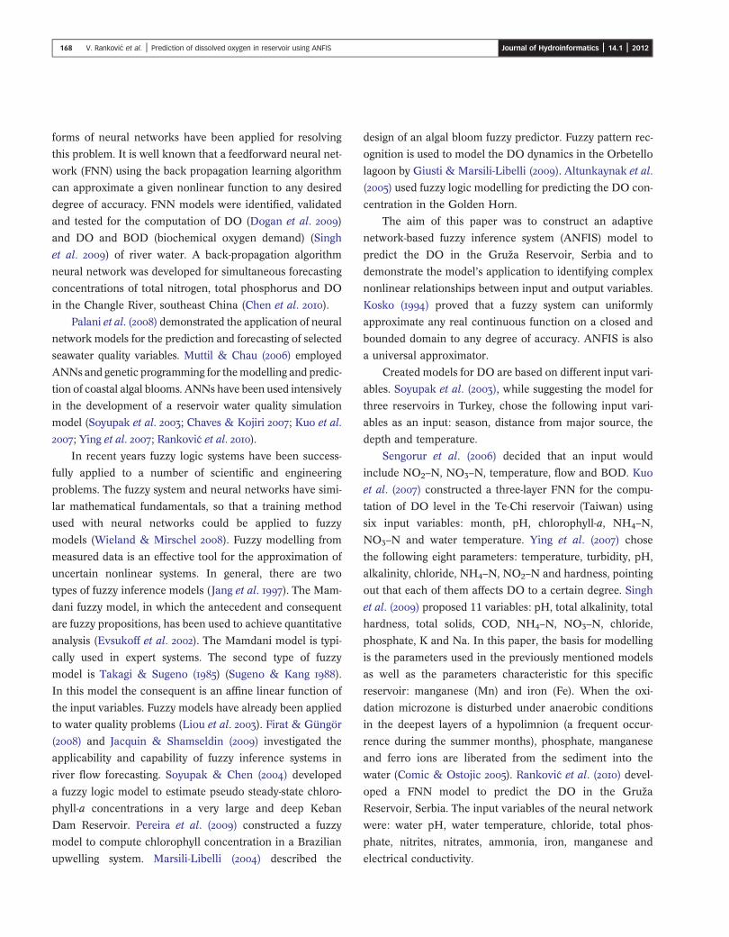
The corresponding equivalent ANFIS architecture (Jang

) is shown in Figure 2. When fk is a constant, a zero-order

Takagi–Sugeno fuzzy model is formed, which may be con-

sidered to be a special case of a Mamdani FIS. The zero-order

Figure 2 | Two-input ANFIS with four rules.

Takagi–Sugeno fuzzy model is functionally equivalent to a

radial basis function (RBF) network under certain constraints.

Functional equivalence between a RBF network and

ANFIS can be established under these conditions (Jang &

Sun ).

1. The number of RBF hidden neurons is equal to the

number of fuzzy if–then rules.

2. The output of each fuzzy if–then rule is composed of a

constant.

3. The membership functions (MFs) within each fuzzy rule

are chosen as Gaussian functions with the same variance.

4. The multiplication operator is used to compute the firing

strength of each rule.

5. Both the RBF network and the FIS under consideration

use the same method (i.e. either weighted average or

weighted sum) to derive their overall outputs.

In this study, the third constraint is not satisfied because

the gauss2mf membership function, but not Gaussian func-

tion, is selected.

The ANFIS structure contains five layers.

Layer 1

The outputs of the layer are fuzzymembership grade of inputs

μAijðxjÞ. If the Gaussian MF is adopted, μAij

ðxjÞ is given by:

μAijðxjÞ ¼ e�ðxj � cijÞ=2σ2

ij ; i ¼ 1;2; j ¼ 1;2; ð1Þ

where cij and σij are the parameters of the MF or premise

parameters.

Layer 2

Every node in this layer is a fixed node. The output of nodes

can be presented as:

u1 ¼ μA11ðx1Þ�μA12

ðx2Þ;u2 ¼ μA11

ðx1Þ�μA22ðx2Þ;

u3 ¼ μA21ðx1Þ�μA12

ðx2Þ;u4 ¼ μA21

ðx1Þ�μA22ðx2Þ;

� denotes T-norm. Nodes are marked by a circle and

labelled ∏.


Layer 3

The output of each fixed node labelled N can be presented

as:

�uk ¼ ukP4k¼1 uk

; k ¼ 1; 2; 3; 4: ð2Þ

Layer 4

Every node in this layer is a square. The outputs of this layer

are given by:

�ukfk ¼ �uk

X2j¼1

qkjxj þ ck; k ¼ 1;2;3;4: ð3Þ

Layer 5

Finally, the output of the ANFIS can be presented as:

y ¼X4k¼1

�ukfk ¼ 1P4k¼1 uk

X4k¼1

uk

X2j¼1

qkjxj þ ck

0@

1A: ð4Þ

There are four methods to update the parameters of the

ANFIS structure, as listed below according to their compu-

tation complexities (Jang ):

1. Gradient descent (GD): All parameters are updated by

the GD.

2. GD and one pass of least square estimation (LSE): The

LSE is applied only once at the very beginning to get

the initial values of the consequent parameters and

then the GD takes over to update all parameters.

3. GD and LSE: This is the hybrid learning.

4. Sequential LSE: using extended Kalman filter algorithm

to update all parameters.

In this paper the hybrid learning algorithm that com-

bines the GD and the LSE method is used for updating

the parameters. For adapting premise parameters the GD

method is used. The LSE method is used for updating the

consequent parameters. Each epoch of the hybrid learning

algorithm involves a forward and a backward pass in the

ANFIS. Jang () described the mathematical background

of the hybrid learning algorithm. This algorithm converges

much faster since it reduces the dimension of the search

space of the back-propagation GD algorithm.

Select input variables and performance criteria

The selection of an appropriate set of input variables from

all possible input variables during AI model development

is important for obtaining high-quality model. Many of the

described methods for input variable selection are based

on heuristics, expert knowledge, statistical analysis, or a

combination of these. However, although there is a well

justified need to consider input variable selection carefully,

there is currently no consensus on how this task should be

undertaken (May et al. ).

Jang () presented a heuristic, relatively simple and fast

method of input selection for neuro-fuzzy modelling using

ANFIS. Finding an optimal solution requires building ANFIS

models for each possible combination of input variables (the

number of possible combinations is 2nc , where nc is the

number of candidate variables) which becomes computation-

ally prohibitive for problems involving even a moderate

number of candidate input variables. If we have a modelling

problem with nc candidate inputs and we want to find the

most influentialm inputs as the inputs to ANFIS, we construct

Cncm ¼ ncðnc � 1Þ . . . ðnc �mþ 1Þ=m ANFIS models (each

with different combination of m inputs), and train them with

a single pass of the LSE method (Jang ). The proposed

method is based on the assumption that the ANFIS model

with the smallest root mean squared error (RMSE) after one

epoch of training has a greater potential of achieving a lower

RMSE when more epochs of training are given. This assump-

tion is not absolutely true, but it is heuristically reasonable.

In this paper, Jang’s method was used for the selection

of an appropriate set of input variables. An ANFIS model

has been trained for 300 epochs. After that number of

epochs, the reduction of the RMSE value is negligible.

Thus, comparison of trained ANFIS models is justified.

RMSE is calculated by the following expression:

RMSE ¼ffiffiffiffiffiffiffiffiffiffiffiffiffiffiffiffiffiffiffiffiffiffiffiffiffiffiffiffiffiffiffiffiffiffiffiffiffi1No

XNo

i¼1

ðymi � yiÞ2vuut ; ð5Þ

where yi and ymi denote the network output and measured

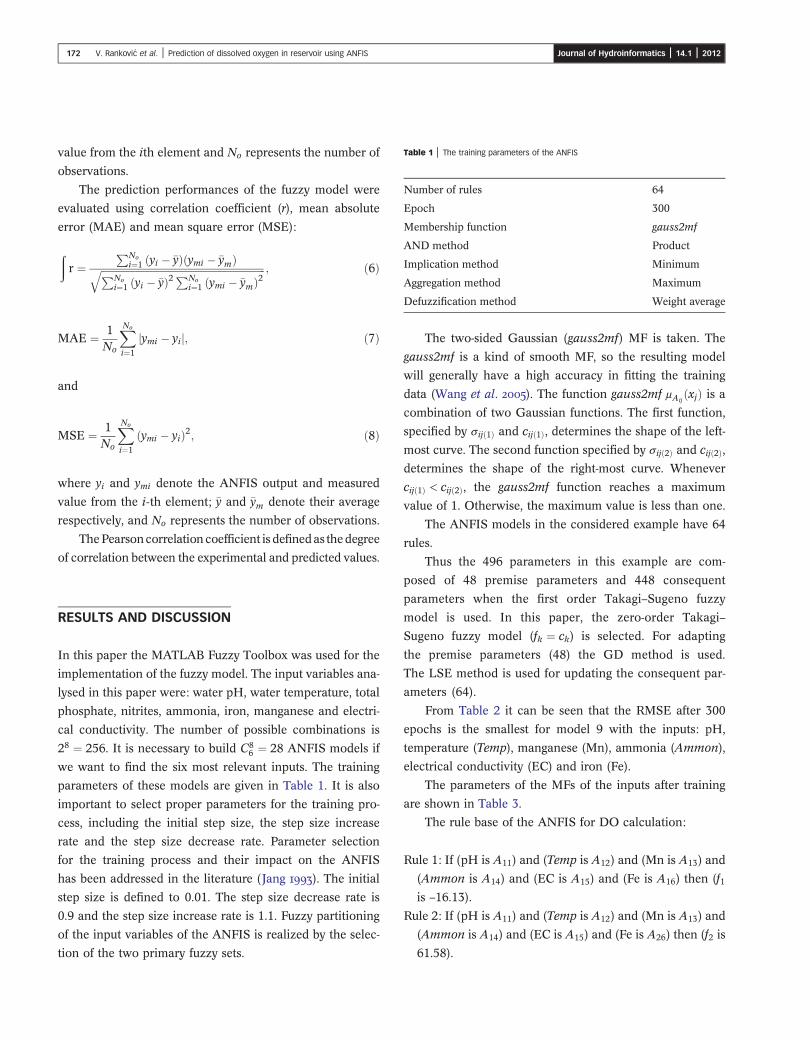
Table 1 | The training parameters of the ANFIS

Number of rules 64

Epoch 300

Membership function gauss2mf

AND method Product

Implication method Minimum

Aggregation method Maximum

Defuzzification method Weight average


value from the ith element and No represents the number of

observations.

The prediction performances of the fuzzy model were

evaluated using correlation coefficient (r), mean absolute

error (MAE) and mean square error (MSE):

ðr ¼

PNoi¼1 ðyi � �yÞðymi � �ymÞffiffiffiffiffiffiffiffiffiffiffiffiffiffiffiffiffiffiffiffiffiffiffiffiffiffiffiffiffiffiffiffiffiffiffiffiffiffiffiffiffiffiffiffiffiffiffiffiffiffiffiffiffiffiffiffiffiffiffiffiffiffiffiffiffiffiPNo

i¼1 ðyi � �yÞ2 PNoi¼1 ðymi � �ymÞ2

q ; ð6Þ

MAE ¼ 1No

XNo

i¼1

jymi � yij; ð7Þ

and

MSE ¼ 1No

XNo

i¼1

ðymi � yiÞ2; ð8Þ

where yi and ymi denote the ANFIS output and measured

value from the i-th element; �y and �ym denote their average

respectively, and No represents the number of observations.

ThePearsoncorrelation coefficient is definedas thedegree

of correlation between the experimental and predicted values.

RESULTS AND DISCUSSION

In this paper the MATLAB Fuzzy Toolbox was used for the

implementation of the fuzzy model. The input variables ana-

lysed in this paper were: water pH, water temperature, total

phosphate, nitrites, ammonia, iron, manganese and electri-

cal conductivity. The number of possible combinations is

28 ¼ 256. It is necessary to build C86 ¼ 28 ANFIS models if

we want to find the six most relevant inputs. The training

parameters of these models are given in Table 1. It is also

important to select proper parameters for the training pro-

cess, including the initial step size, the step size increase

rate and the step size decrease rate. Parameter selection

for the training process and their impact on the ANFIS

has been addressed in the literature (Jang ). The initial

step size is defined to 0.01. The step size decrease rate is

0.9 and the step size increase rate is 1.1. Fuzzy partitioning

of the input variables of the ANFIS is realized by the selec-

tion of the two primary fuzzy sets.

The two-sided Gaussian (gauss2mf) MF is taken. The

gauss2mf is a kind of smooth MF, so the resulting model

will generally have a high accuracy in fitting the training

data (Wang et al. ). The function gauss2mf μAijðxjÞ is a

combination of two Gaussian functions. The first function,

specified by σijð1Þ and cijð1Þ, determines the shape of the left-

most curve. The second function specified by σijð2Þ and cijð2Þ,

determines the shape of the right-most curve. Whenever

cijð1Þ < cijð2Þ, the gauss2mf function reaches a maximum

value of 1. Otherwise, the maximum value is less than one.

The ANFIS models in the considered example have 64

rules.

Thus the 496 parameters in this example are com-

posed of 48 premise parameters and 448 consequent

parameters when the first order Takagi–Sugeno fuzzy

model is used. In this paper, the zero-order Takagi–

Sugeno fuzzy model (fk ¼ ck) is selected. For adapting

the premise parameters (48) the GD method is used.

The LSE method is used for updating the consequent par-

ameters (64).

From Table 2 it can be seen that the RMSE after 300

epochs is the smallest for model 9 with the inputs: pH,

temperature (Temp), manganese (Mn), ammonia (Ammon),

electrical conductivity (EC) and iron (Fe).

The parameters of the MFs of the inputs after training

are shown in Table 3.

The rule base of the ANFIS for DO calculation:

Rule 1: If (pH is A11) and (Temp is A12) and (Mn is A13) and

(Ammon is A14) and (EC is A15) and (Fe is A16) then (f1is –16.13).


(Ammon is A14) and (EC is A15) and (Fe is A26) then (f2 is

61.58).

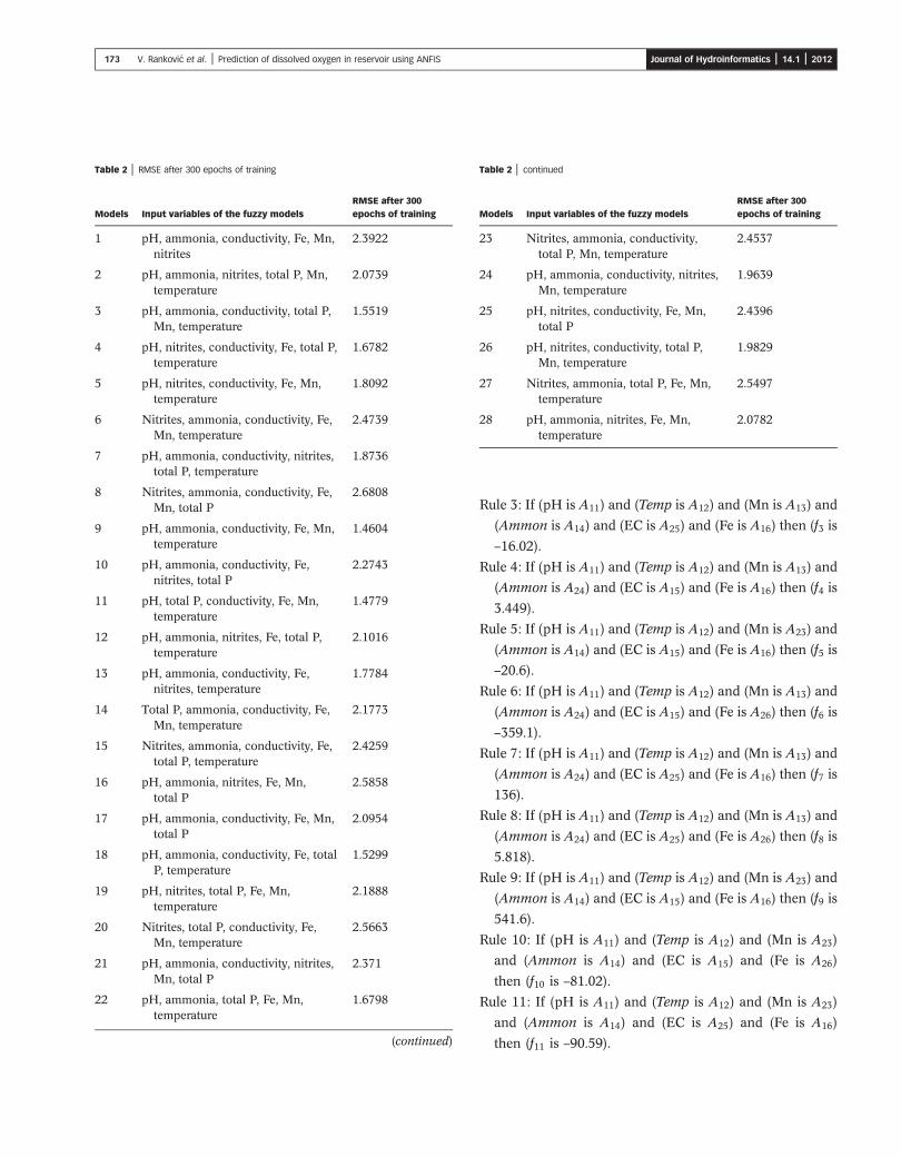
Table 2 | RMSE after 300 epochs of training

Models Input variables of the fuzzy modelsRMSE after 300epochs of training

1 pH, ammonia, conductivity, Fe, Mn,nitrites

2.3922

2 pH, ammonia, nitrites, total P, Mn,temperature

2.0739

3 pH, ammonia, conductivity, total P,Mn, temperature

1.5519

4 pH, nitrites, conductivity, Fe, total P,temperature

1.6782

5 pH, nitrites, conductivity, Fe, Mn,temperature

1.8092

6 Nitrites, ammonia, conductivity, Fe,Mn, temperature

2.4739

7 pH, ammonia, conductivity, nitrites,total P, temperature

1.8736

8 Nitrites, ammonia, conductivity, Fe,Mn, total P

2.6808

9 pH, ammonia, conductivity, Fe, Mn,temperature

1.4604

10 pH, ammonia, conductivity, Fe,nitrites, total P

2.2743

11 pH, total P, conductivity, Fe, Mn,temperature

1.4779

12 pH, ammonia, nitrites, Fe, total P,temperature

2.1016

13 pH, ammonia, conductivity, Fe,nitrites, temperature

1.7784

14 Total P, ammonia, conductivity, Fe,Mn, temperature

2.1773

15 Nitrites, ammonia, conductivity, Fe,total P, temperature

2.4259

16 pH, ammonia, nitrites, Fe, Mn,total P

2.5858

17 pH, ammonia, conductivity, Fe, Mn,total P

2.0954

18 pH, ammonia, conductivity, Fe, totalP, temperature

1.5299

19 pH, nitrites, total P, Fe, Mn,temperature

2.1888

20 Nitrites, total P, conductivity, Fe,Mn, temperature

2.5663

21 pH, ammonia, conductivity, nitrites,Mn, total P

2.371

22 pH, ammonia, total P, Fe, Mn,temperature

1.6798

(continued)

Table 2 | continued

Models Input variables of the fuzzy modelsRMSE after 300epochs of training

23 Nitrites, ammonia, conductivity,total P, Mn, temperature

2.4537

24 pH, ammonia, conductivity, nitrites,Mn, temperature

1.9639

25 pH, nitrites, conductivity, Fe, Mn,total P

2.4396

26 pH, nitrites, conductivity, total P,Mn, temperature

1.9829

27 Nitrites, ammonia, total P, Fe, Mn,temperature

2.5497

28 pH, ammonia, nitrites, Fe, Mn,temperature

2.0782




–16.02).



3.449).



–20.6).



–359.1).



136).



5.818).



541.6).

Rule 10: If (pH is A11) and (Temp is A12) and (Mn is A23)

and (Ammon is A14) and (EC is A15) and (Fe is A26)

then (f10 is –81.02).



then (f11 is –90.59).

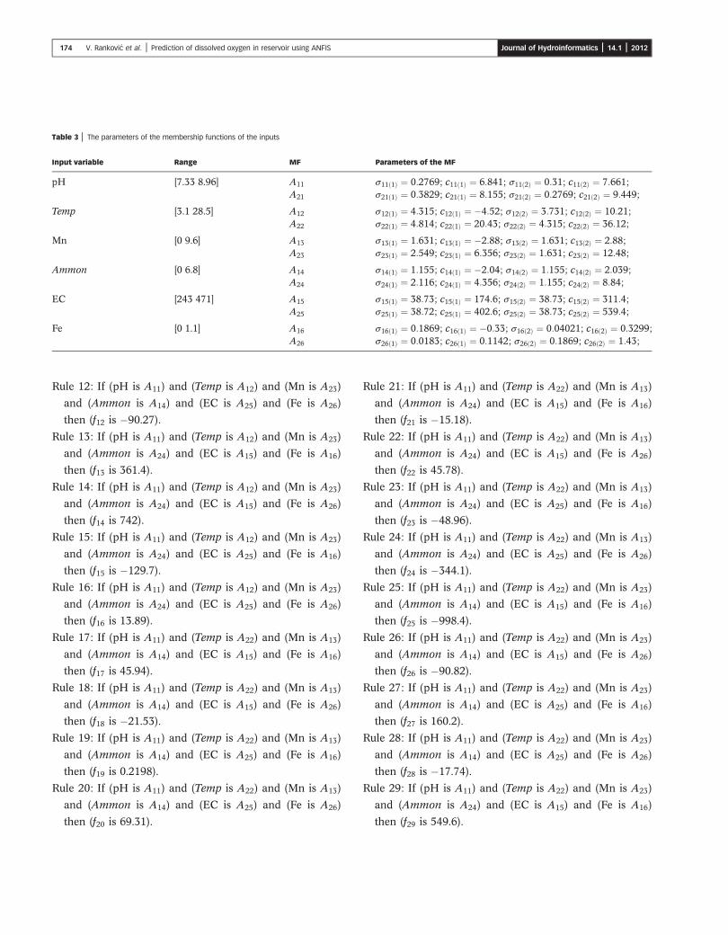
Table 3 | The parameters of the membership functions of the inputs

Input variable Range MF Parameters of the MF

pH [7.33 8.96] A11 σ11ð1Þ ¼ 0:2769; c11ð1Þ ¼ 6:841; σ11ð2Þ ¼ 0:31; c11ð2Þ ¼ 7:661;A21 σ21ð1Þ ¼ 0:3829; c21ð1Þ ¼ 8:155; σ21ð2Þ ¼ 0:2769; c21ð2Þ ¼ 9:449;

Temp [3.1 28.5] A12 σ12ð1Þ ¼ 4:315; c12ð1Þ ¼ �4:52; σ12ð2Þ ¼ 3:731; c12ð2Þ ¼ 10:21;A22 σ22ð1Þ ¼ 4:814; c22ð1Þ ¼ 20:43; σ22ð2Þ ¼ 4:315; c22ð2Þ ¼ 36:12;

Mn [0 9.6] A13 σ13ð1Þ ¼ 1:631; c13ð1Þ ¼ �2:88; σ13ð2Þ ¼ 1:631; c13ð2Þ ¼ 2:88;A23 σ23ð1Þ ¼ 2:549; c23ð1Þ ¼ 6:356; σ23ð2Þ ¼ 1:631; c23ð2Þ ¼ 12:48;

Ammon [0 6.8] A14 σ14ð1Þ ¼ 1:155; c14ð1Þ ¼ �2:04; σ14ð2Þ ¼ 1:155; c14ð2Þ ¼ 2:039;A24 σ24ð1Þ ¼ 2:116; c24ð1Þ ¼ 4:356; σ24ð2Þ ¼ 1:155; c24ð2Þ ¼ 8:84;

EC [243 471] A15 σ15ð1Þ ¼ 38:73; c15ð1Þ ¼ 174:6; σ15ð2Þ ¼ 38:73; c15ð2Þ ¼ 311:4;A25 σ25ð1Þ ¼ 38:72; c25ð1Þ ¼ 402:6; σ25ð2Þ ¼ 38:73; c25ð2Þ ¼ 539:4;

Fe [0 1.1] A16 σ16ð1Þ ¼ 0:1869; c16ð1Þ ¼ �0:33; σ16ð2Þ ¼ 0:04021; c16ð2Þ ¼ 0:3299;A26 σ26ð1Þ ¼ 0:0183; c26ð1Þ ¼ 0:1142; σ26ð2Þ ¼ 0:1869; c26ð2Þ ¼ 1:43;




then (f12 is �90.27).



then (f13 is 361.4).



then (f14 is 742).



then (f15 is �129.7).



then (f16 is 13.89).



then (f17 is 45.94).



then (f18 is �21.53).



then (f19 is 0.2198).



then (f20 is 69.31).



then (f21 is �15.18).



then (f22 is 45.78).



then (f23 is �48.96).



then (f24 is �344.1).



then (f25 is �998.4).



then (f26 is �90.82).



then (f27 is 160.2).



then (f28 is �17.74).



then (f29 is 549.6).




then (f30 is 216.3).



then (f31 is 298.3).



then (f32 is �18.93).



then (f33 is 27.98).



then (f34 is 61.26).



then (f35 is 190.2).



then (f36 is �117.2).



then (f37 is 114.8).



then (f38 is �249.8).



then (f39 is �1460).



then (f40 is 773.2).



then (f41 is �590.5).



then (f42 is �420.6).



then (f43 is 270).



then (f44 is 490.9).



then (f45 is 22).



then (f46 is 112.6).



then (f47 is �30.23).



then (f48 is 182.5).



then (f49 is 4.394).



then (f50 is �74.94).



then (f51 is �59.17).



then (f52 is �174).



then (f53 is �91.47).



then (f54 is 715.3).



then (f55 is 927.3).



then (f56 is 1016).



then (f57 is 327.9).

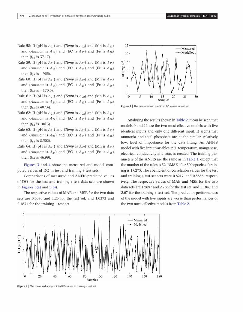
Figure 3 | The measured and predicted DO values in test set.




then (f58 is 37.17).



then (f59 is �966).



then (f60 is �170.6).



then (f61 is 407.4).



then (f62 is 106.3).



then (f63 is 8.502).



then (f64 is 46.99).

Figures 3 and 4 show the measured and model com-

puted values of DO in test and trainingþ test sets.

Comparisons of measured and ANFIS-predicted values

of DO for the test and trainingþ test data sets are shown

in Figures 5(a) and 5(b)).

The respective values of MAE and MSE for the two data

sets are 0.6670 and 1.23 for the test set, and 1.0373 and

2.1831 for the trainingþ test set.

Figure 4 | The measured and predicted DO values in trainingþ test set.

Analysing the results shown in Table 2, it can be seen that

models 9 and 11 are the two most effective models with five

identical inputs and only one different input. It seems that

ammonia and total phosphate are at the similar, relatively

low, level of importance for the data fitting. An ANFIS

model with five input variables: pH, temperature, manganese,

electrical conductivity and iron, is created. The training par-

ameters of the ANFIS are the same as in Table 1, except that

the number of the rules is 32. RMSE after 300 epochs of train-

ing is 1.6275. The coefficient of correlation values for the test

and trainingþ test set sets were 0.8217, and 0.8856, respect-

ively. The respective values of MAE and MSE for the two

data sets are 1.2897 and 2.786 for the test set, and 1.1847 and

2.67 for the trainingþ test set. The prediction performances

of the model with five inputs are worse than performances of

the two most effective models from Table 2.

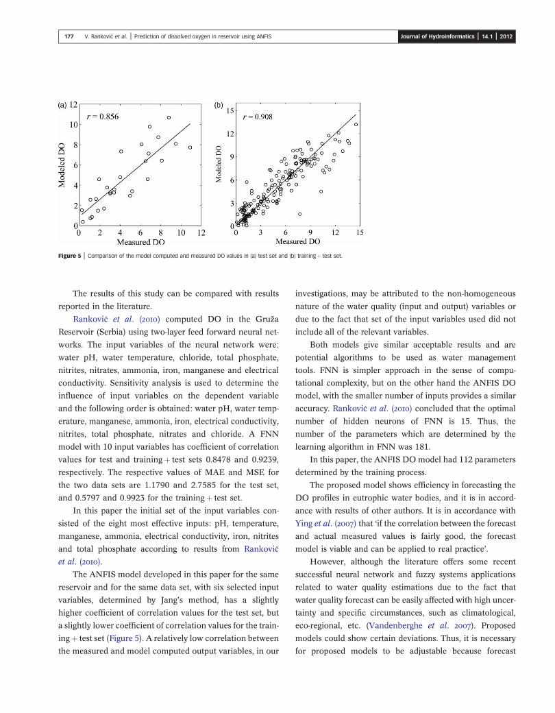
Figure 5 | Comparison of the model computed and measured DO values in (a) test set and (b) trainingþ test set.


The results of this study can be compared with results

reported in the literature.

Rankovic et al. () computed DO in the Gruža

Reservoir (Serbia) using two-layer feed forward neural net-

works. The input variables of the neural network were:

water pH, water temperature, chloride, total phosphate,

nitrites, nitrates, ammonia, iron, manganese and electrical

conductivity. Sensitivity analysis is used to determine the

influence of input variables on the dependent variable

and the following order is obtained: water pH, water temp-

erature, manganese, ammonia, iron, electrical conductivity,

nitrites, total phosphate, nitrates and chloride. A FNN

model with 10 input variables has coefficient of correlation

values for test and trainingþ test sets 0.8478 and 0.9239,

respectively. The respective values of MAE and MSE for

the two data sets are 1.1790 and 2.7585 for the test set,

and 0.5797 and 0.9923 for the trainingþ test set.

In this paper the initial set of the input variables con-

sisted of the eight most effective inputs: pH, temperature,

manganese, ammonia, electrical conductivity, iron, nitrites

and total phosphate according to results from Rankovic

et al. ().

The ANFIS model developed in this paper for the same

reservoir and for the same data set, with six selected input

variables, determined by Jang’s method, has a slightly

higher coefficient of correlation values for the test set, but

a slightly lower coefficient of correlation values for the train-

ingþ test set (Figure 5). A relatively low correlation between

the measured and model computed output variables, in our

investigations, may be attributed to the non-homogeneous

nature of the water quality (input and output) variables or

due to the fact that set of the input variables used did not

include all of the relevant variables.

Both models give similar acceptable results and are

potential algorithms to be used as water management

tools. FNN is simpler approach in the sense of compu-

tational complexity, but on the other hand the ANFIS DO

model, with the smaller number of inputs provides a similar

accuracy. Rankovic et al. () concluded that the optimal

number of hidden neurons of FNN is 15. Thus, the

number of the parameters which are determined by the

learning algorithm in FNN was 181.

In this paper, the ANFIS DO model had 112 parameters

determined by the training process.

The proposed model shows efficiency in forecasting the

DO profiles in eutrophic water bodies, and it is in accord-

ance with results of other authors. It is in accordance with

Ying et al. () that ‘if the correlation between the forecast

and actual measured values is fairly good, the forecast

model is viable and can be applied to real practice’.

However, although the literature offers some recent

successful neural network and fuzzy systems applications

related to water quality estimations due to the fact that

water quality forecast can be easily affected with high uncer-

tainty and specific circumstances, such as climatological,

eco-regional, etc. (Vandenberghe et al. ). Proposed

models could show certain deviations. Thus, it is necessary

for proposed models to be adjustable because forecast


model is time-bound and therefore it is necessary to update

the model from time to time with actual measured values

(Ying et al. ).

CONCLUSIONS

The aim of this paper was to develop an ANFIS model to

predict the DO in water supply reservoir Gruža in Serbia

and demonstrate its application to identify complex non-

linear relationships between input and output variables.

The proposed model shows efficiency in forecasting the

DO profiles in eutrophic water bodies. Also, the model is

an invaluable tool for studying system dynamics and pre-

dicting future states. The fuzzy logic model once

developed for a water body, can favourably be used during

further monitoring activities, as a predictive management

tool. It can be concluded that neuro-fuzzy modelling can

be successfully applied for estimations in lakes and reser-

voirs, and can replace classical approaches, because of its

simplicity. An ANFIS application could be used in the

future to investigate the applicability of this approach to

other reservoirs. As a final conclusion, ANFIS can be a

powerful tool for environmental and ecological modelling

and assessment.

It should be noted that there are no fixed rules for devel-

oping AI techniques in the fields of water quality prediction

and forecasting. AI models are usually constructed based on

expert knowledge and trial and error adjustment of par-

ameters. Thus, there is no guarantee that the optimal

solution will be found. Some future directions for further

development are the hybrid combinations of two or more

AI methods to produce an even better water quality model-

ling system.

ACKNOWLEDGEMENT

The authors would like to express their sincere thanks to the

three anonymous referees for their valuable comments and

useful suggestions that helped to improve this paper and

future research.

REFERENCES

Altunkaynak, A., Özger, M. & Çakmakcı, M. Fuzzy logicmodeling of the dissolved oxygen fluctuations in GoldenHorn. Ecol. Model. 189 (3–4), 436–446.

Antonopoulos, V. Z. & Gianniou, S. K. Simulation of watertemperature and dissolved oxygen distribution in the LakeVegoritis, Greece. Ecol. Model. 160 (1–2), 39–53.

Chaves, P. & Kojiri, T. Conceptual fuzzy neural networkmodel for water quality simulation. Hydrol. Process. 21 (5),634–646.

Chen, Q., Morales-Chaves, Y., Li, H. & Mynett, A. E. Hydroinformatics techniques in eco-environmentalmodelling and management. J. Hydroinform. 8 (4), 297–316.

Chen, D., Lu, J. & Shen, Y. Artificial neural networkmodelling of concentrations of nitrogen, phosphorus anddissolved oxygen in a non-point source polluted river inZhejiang Province, southeast China. Hydrol. Process. 24 (3),290–299.

Chon, T. S. & Park, Y. S. Ecological informatics as anadvanced interdisciplinary interpretation of ecosystems.Ecol. Inform. 1 (3), 213–217.

Lj Comic &A. Ostojic (eds). The Gruža Reservoir (in Serbian).Faculty of Science, Kragujevac, Serbia and Montenegro.

Dogan, E., Sengorur, B. & Koklu, R. Modeling biologicaloxygen demand of the Melen River in Turkey using anartificial neural network technique. J. Environ. Manag. 90 (2),1229–1235.

Evsukoff, A., Branco, A. C. S. & Galichet, S. Structureidentification and parameter optimization for non-linearfuzzy modeling. Fuzzy Sets Sys. 132 (2), 173–188.

Firat, M. & Güngör, M. Hydrological time-series modellingusing an adaptive neuro-fuzzy inference system. Hydrol.Process. 22 (13), 2122–2132.

Giusti, E. & Marsili-Libelli, S. Spatio-temporal dissolvedoxygen dynamics in the Orbetello lagoon by fuzzy patternrecognition. Ecol. Model. 220 (19), 2415–2426.

Jacquin, A. P. & Shamseldin, A. Y. Review of the applicationof fuzzy inference systems in river flow forecasting.J. Hydroinform. 11 (3–4), 202–210.

Jang, J. S. R. ANFIS:Adaptive-Network-Based Fuzzy InferenceSystems. IEEE Trans. Syst. Man Cybernet. 23 (3), 665–685.

Jang, J. S. R. Input selection for ANFIS learning. InProceedings of the Fifth IEEE International Conference onFuzzy Systems, New Orleans, LA, September (IEEE NeuralNetworks Council, ed.), pp. 1493–1499.

Jang, J. S. R. & Sun, C. T. Functional equivalence betweenradial basis function networks and fuzzy inference systems.IEEE Trans. Neur. Net. 4 (1), 156–159.

Jang, J. S. R., Sun, C. T. & Mizutani, E. Neuro-Fuzzy and SoftComputing: A Computational Approach to Learning andMachine Intelligence. Prentice-Hall, Upper Saddle River, NJ.

Kosko, B. Fuzzy Systems as universal approximators. IEEETrans. Comp. 43 (11), 1329–1333.

http://dx.doi.org/10.1016/j.ecolmodel.2005.03.007



http://dx.doi.org/10.1016/S0304-3800(02)00286-7

http://dx.doi.org/10.1016/S0304-3800(02)00286-7

http://dx.doi.org/10.1016/S0304-3800(02)00286-7

http://dx.doi.org/10.1002/hyp.6279


http://dx.doi.org/10.2166/hydro.2006.011


http://dx.doi.org/10.1016/j.ecoinf.2006.02.007

http://dx.doi.org/10.1016/j.ecoinf.2006.02.007

http://dx.doi.org/10.1016/j.jenvman.2008.06.004



http://dx.doi.org/10.1016/S0165-0114(02)00111-2

http://dx.doi.org/10.1016/S0165-0114(02)00111-2

http://dx.doi.org/10.1016/S0165-0114(02)00111-2








http://dx.doi.org/10.1109/72.182710

http://dx.doi.org/10.1109/72.182710

http://dx.doi.org/10.1109/12.324566


Kuo, J. T., Hsieh, M. H., Lung, W. S. & She, N. Usingartificial neural network for reservoir eutrophicationprediction. Ecol. Model. 200 (1–2), 171–177.

Lin, J. Y., Cheng, C. T. & Chau, K. W. Using support vectormachines for long-term discharge prediction. Hydrol. Sci. J.51 (4), 599–612.

Liou, S. M., Lo, S. L. & Hu, C. Y. Application of two-stagefuzzy set theory to river quality evaluation in Taiwan. WaterRes. 37 (6), 1406–1416.

Marsili-Libelli, S. Fuzzy prediction of the algal blooms in theOrbetello lagoon. Environ. Model. Softw. 19 (9), 799–808.

May, R. J., Maier, H. R., Dandy, G. C. & Fernando, T. M. K. G

Non-linear variable selection for artificial neural networksusing partial mutual information. Environ. Model. Software23 (10–11), 1312–1326.

Muttil, N. & Chau, K. W. Neural network and geneticprogramming for modelling coastal algal blooms. Int. J.Environ. Pollut. 28 (3–4), 223–238.

Ostojic, A., Curcic, S., Comic, Lj. & Topuzovic, M. Estimateof the eutrophication process in the Gruža Reservoir(Serbia and Montenegro). Acta Hydrochim. Hydrobiol. 33 (6),605–613.

Palani, S., Liong, S. Y. & Tkalich, P. An ANN application forwater quality forecasting.MarinePollut. Bull.56 (9), 1586–1597.

Pereira, G. C., Evsukoff, A. & Ebecken, N. F. F. Fuzzymodelling of chlorophyll production in a Brazilian upwellingsystem. Ecol. Model. 220 (12), 1506–1512.

Rankovic , V., Radulovic , J., Radojevic, I., Ostojic , A. & Comic, Lj. Neural network modeling of dissolved oxygen in theGruža reservoir, Serbia. Ecol. Model. 221 (8), 1239–1244.

Sengorur, B., Dogan, E., Koklu, R. & Samandar, A. Dissolvedoxygen estimation using artificial neural network for waterquality control. Fresen. Environ. Bull. 15 (9a), 1064–1067.

Singh, K. P., Basant, A., Malik, A. & Jain, G. Artificial neuralnetwork modeling of the river water quality – a case study.Ecol. Model. 220 (6), 888–895.

Soyupak, S. & Chen, D. G. Fuzzy logic model to estimateseasonal pseudo steady state chlorophyll-a concentrations inreservoirs. Environ. Model. Assess. 9 (1), 51–59.

Soyupak, S., Karaer, F., Gürbüz, H., Kivrak, E., Sentürk, E. &Yazici, A. A neural network-based approach forcalculating dissolved oxygen profiles in reservoirs. NeuralComput. Appl. 12 (3–4), 166–172.

Sugeno, M. & Kang, G. T. Structure identification of fuzzymodel. Fuzzy Sets Syst. 28 (1), 15–33.

Takagi, T. & Sugeno, M. Fuzzy identification of systems andits applications to modeling and control. IEEE Trans. Syst.Man Cybern. 15 (1), 116–132.

Vandenberghe, V., Bauwens, W. & Vanrolleghem, P. A. Evaluation of uncertainty propagation into river waterquality predictions to guide future monitoring campaigns.Environ. Model. Software 22 (5), 725–732.

Wang, H., Kwong, S., Jinb, Y., Wei, W. & Mand, K. F. Multi-objective hierarchical genetic algorithm for interpretablefuzzy rule-based knowledge extraction. Fuzzy Set. Syst.149 (1), 149–186.

Wang, W. C., Chau, K. W., Cheng, C. T. & Qiu, L. Acomparison of performance of several artificial intelligencemethods for forecasting monthly discharge time series.J. Hydrol. 374 (3–4), 294–306.

Wieland, R. & Mirschel, W. Adaptive fuzzy modeling versusartificial neural networks. Environ. Model. Software 23 (2),215–224.

Ying, Z., Jun, N., Fuyi, C. & Liang, G. Water quality forecastthrough application of BP neural network at Yuquioreservoir. J. Zhejiang Univ. Sci. A. 8 (9), 1482–1487.

First received 15 June 2010; accepted in revised form 16 December 2010. Available online 23 April 2011




http://dx.doi.org/10.1623/hysj.51.4.599

http://dx.doi.org/10.1623/hysj.51.4.599

http://dx.doi.org/10.1016/S0043-1354(02)00479-7

http://dx.doi.org/10.1016/S0043-1354(02)00479-7

http://dx.doi.org/10.1016/j.envsoft.2003.03.008




http://dx.doi.org/10.1504/IJEP.2006.011208

http://dx.doi.org/10.1504/IJEP.2006.011208

http://dx.doi.org/10.1002/aheh.200500601



http://dx.doi.org/10.1016/j.marpolbul.2008.05.021

http://dx.doi.org/10.1016/j.marpolbul.2008.05.021








http://dx.doi.org/10.1023/B:ENMO.0000020890.57185.92



http://dx.doi.org/10.1007/s00521-003-0378-8

http://dx.doi.org/10.1007/s00521-003-0378-8

http://dx.doi.org/10.1016/0165-0114(88)90113-3

http://dx.doi.org/10.1016/0165-0114(88)90113-3



http://dx.doi.org/10.1016/j.fss.2004.07.013



http://dx.doi.org/10.1016/j.jhydrol.2009.06.019





prediction of dissolved oxygen in reservoirs using ... · adaptive network-based fuzzy inference...

Documents