Policy Research Working Paper 6208

India’s Economic Growth and Environmental Sustainability

What Are the Tradeoffs?

Muthukumara ManiAnil Markandya

Aarsi SagarSebnem Sahin

The World BankSouth Asia RegionDisaster Risk Management and Climate ChangeSeptember 2012

WPS6208P

ublic

Dis

clos

ure

Aut

horiz

edP

ublic

Dis

clos

ure

Aut

horiz

edP

ublic

Dis

clos

ure

Aut

horiz

edP

ublic

Dis

clos

ure

Aut

horiz

ed

Produced by the Research Support Team

Abstract

The Policy Research Working Paper Series disseminates the findings of work in progress to encourage the exchange of ideas about development issues. An objective of the series is to get the findings out quickly, even if the presentations are less than fully polished. The papers carry the names of the authors and should be cited accordingly. The findings, interpretations, and conclusions expressed in this paper are entirely those of the authors. They do not necessarily represent the views of the International Bank for Reconstruction and Development/World Bank and its affiliated organizations, or those of the Executive Directors of the World Bank or the governments they represent.

Policy Research Working Paper 6208

One of the key environmental problems facing India is that of particle pollution from the combustion of fossil fuels. This has serious health consequences and with the rapid growth in the economy these impacts are increasing. At the same time, economic growth is an imperative and policy makers are concerned about the possibility that pollution reduction measures could reduce growth significantly. This paper addresses the tradeoffs involved in controlling local pollutants such as particles. Using an established Computable General Equilibrium model, it evaluates the impacts of a tax on coal or on emissions of particles such that these instruments result in emission

This paper is a product of the Disaster Risk Management and Climate Change, South Asia Region. It is part of a larger effort by the World Bank to provide open access to its research and make a contribution to development policy discussions around the world. Policy Research Working Papers are also posted on the Web at http://econ.worldbank.org. The author may be contacted at mmani@worldbank.org.

levels that are respectively 10 percent and 30 percent lower than they otherwise would be in 2030. The main findings are as follows: (i) A 10 percent particulate emission reduction results in a lower gross domestic product but the size of the reduction is modest; (ii) losses in gross domestic proudct from the tax are partly offset by the health gains from lower particle emissions; (iii) the taxes reduce emissions of carbon dioxide by about 590 million tons in 2030 in the case of the 10 percent reduction and 830 million tons in the case of the 30 percent reduction; and (iv) taken together, the carbon dioxide reduction and the health benefits are greater than the loss of gross domestic product in both cases.

India’s Economic Growth and Environmental

Sustainability: What Are the Tradeoffs?

Muthukumara Mani

Anil Markandya

Aarsi Sagar

Sebnem Sahin12

JEL codes: C68, O44, O53, Q43, Q52

Key words: India, Energy, Pollution control, Environment Growth and Health, CGE

1 This paper is part of a collaborative effort between the World Bank and the Ministry of Environment

and Forests (MoEF). Authors extend special gratitude to Mr. Hem Pande (Joint Secretary, MoEF), and his

team for support and guidance throughout the study. The team gratefully acknowledges the contribution

of Dan Biller, Charles Cormier, Giovanna Prennushi, and Michael Toman for carefully reviewing and

providing expert guidance to the team at crucial stages. We also extend our gratitude to Aziz Bouzaher,

Kirk Hamilton and Glen Marie Lange as peer reviewers of the earlier version of the paper. The financial

support of UK‘s Department for International Development (DFID) is gratefully acknowledged.

2 The authors can be contacted at mmani@worldbank.org, World Bank-SASDC,

anil.markandya@bc3research.org, BC3 Basque Center for Climate Change, asagar@post.harvard.edu,

World Bank-SASDI; ssahin@worldbank.org, World Bank-SASDC.

2

Introduction

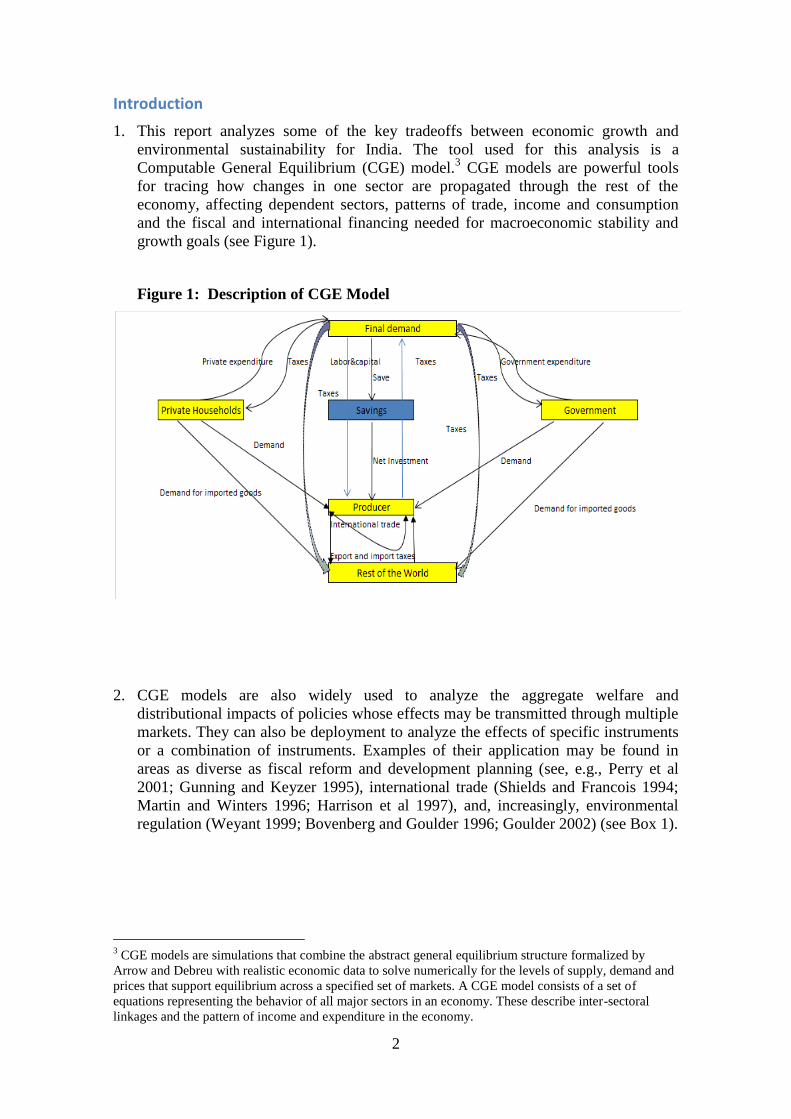
1. This report analyzes some of the key tradeoffs between economic growth and

environmental sustainability for India. The tool used for this analysis is a

Computable General Equilibrium (CGE) model.3 CGE models are powerful tools

for tracing how changes in one sector are propagated through the rest of the

economy, affecting dependent sectors, patterns of trade, income and consumption

and the fiscal and international financing needed for macroeconomic stability and

growth goals (see Figure 1).

Figure 1: Description of CGE Model

2. CGE models are also widely used to analyze the aggregate welfare and

distributional impacts of policies whose effects may be transmitted through multiple

markets. They can also be deployment to analyze the effects of specific instruments

or a combination of instruments. Examples of their application may be found in

areas as diverse as fiscal reform and development planning (see, e.g., Perry et al

2001; Gunning and Keyzer 1995), international trade (Shields and Francois 1994;

Martin and Winters 1996; Harrison et al 1997), and, increasingly, environmental

regulation (Weyant 1999; Bovenberg and Goulder 1996; Goulder 2002) (see Box 1).

3 CGE models are simulations that combine the abstract general equilibrium structure formalized by

Arrow and Debreu with realistic economic data to solve numerically for the levels of supply, demand and

prices that support equilibrium across a specified set of markets. A CGE model consists of a set of

equations representing the behavior of all major sectors in an economy. These describe inter-sectoral

linkages and the pattern of income and expenditure in the economy.

3

Box 1: CGE Models and Environmental Policy

Policies aimed at significantly reducing environmental problems such as global warming,

acid rain, deforestation, waste disposal or any degradation air, water, or soil quality may

imply costs in terms of lower growth of GDP, a reduction in international competitiveness

or in employment. The implied change in relative prices will induce general equilibrium

effects throughout the economy. For this reason, it is useful to evaluate the effects of

environmental policy measures within the framework of a CGE model. Although partial

equilibrium models make it possible to estimate the costs of environmental policy measures,

taking substitution processes in production and consumption as well as market clearing

conditions into account, CGE models additionally allow for adjustments in all sectors,

enabling us to consider the interactions between the intermediate input market and markets

for other commodities or intermediate inputs, and thereby complete the link between factor

incomes and consumer expenditure.

Since the first environmental CGE models appeared (Forsund and Storm, 1988; Dufournaud

et al., 1988), the literature has included applications in many major areas, such as: (a)

models used to evaluate the effects of trade policies or international trade agreements on the

environment (Lucas et al., 1992; Grossman and Krueger, 1993; Madrid-Aris, 1998; Yang,

2001; Beghin et al., 2002) and for diverse applications in the area of the Global Trade

Analysis Project (Hertel, 1997); (b) models to evaluate climate change, which are usually

focused on the stabilization of CO2, NOx and SOx emissions (Bergman, 1991; Jorgenson

and Wilcoxen, 1993; Edwards et al., 2001); (c) models focused on energy issues, which

usually apply energy taxation or pricing to evaluate the impacts that changes in the price of

energy can have on pollution or costs control (Pigott et al., 1992); (d) natural resource

allocation or management models, whose objective is usually the efficient interregional or

inter-sectoral allocation of multi-use natural resources—for example, allocation of water

resources among agriculture, mining, industry, tourism, human consumption and ecological

watersheds (Robinson and Gelhar, 1995; Ianchovichina et al., 2001); and (e) models

focused on evaluating the economic impacts of environmental instruments, or of specific

environmental regulations, such as the Clean Air Act in the USA (Jorgenson and Wilcoxen,

1990; Hazilla and Koop, 1990).

The CGE modeling in India with environmental links has mainly focused on reduction of

carbon emissions and its implications for economic growth (Murthy, Panda and Parikh,

2000; Ohja 2005, 2008). Source: Conrad (2002)

3. The CGE model used here is based on a framework developed and maintained by

the Global Trade Analysis Project (GTAP) network4. GTAP model is built on a

global trade database and reflects, among other indicators, India‘s performance in

terms of export growth, which has increased dramatically during the last decade.

With India emerging as a major producer and exporter of goods including pollution

intensive commodities, the use of such a model to assess the environmental impacts

of the country‘s development path was considered appropriate. The main

environmental variable that has been included in the model is emissions of

particulate matter of less than ten microns (PM10) as well as particles of sulfates

and nitrates). These emissions are recognized among the most important in terms of

their health effects. The standard GTAP model has been expanded to include

emissions from all the key sectors, including PM10 and other small particles

4 https://www.gtap.agecon.purdue.edu/ GTAP (1997), T. Hertel Ed., Global Trade Analysis Modeling and

Applications, NY, USA.

4

emissions originating from fuel use and production activities. A detailed description

of the model, assumptions and corresponding equations is given in Annex 1.

4. This is the first time that a CGE model for India has looked at the trade-offs

between economic growth and ―local‖ pollution mitigation. 5 The open economy

model incorporates links among 57 sectors — various sectors within agriculture,

manufacturing and services — of the Indian economy as well as links between the

economic output of these sectors and air pollution emissions, principally PM10 and

emissions of SO2 and NOx which give rise to health effects. Other CGE models for

India have so far included only 11 to 36 sectors and have not tracked emissions such

as PM10.

5. The model‘s database developed by the GTAP network6 (GTAP database version 8

for 2007) includes data from the India‘s National Accounts. This was complemented

with statistics on urban pollutants (from national statistical sources) and macro-

economic variables (i.e. growth rate projections and total factor productivity (TFP)

from the literature). Specifically, the model was extended by several external

inputs, such as demographics, labor productivity and labor supply, and corrected for

environmental health impacts, sectoral coefficients for PM10 emissions.

Methodology

6. In terms of the methodology, first, an economic growth scenario was developed,

reflecting the most likely path that the Indian economy could follow from 2010

through 2030. This path represents the "economic baseline". The GTAP model was

calibrated to reproduce actual GDP growth rates in the country during 2007-2010

and growth projections in line with World Economic Outlook projections.7 While

the recent IMF survey of the Indian economy suggests a robust 7-8 percent growth

in the next few years in spite of a global economic slowdown, it will be necessary,

according to the IMF, to focus on reinvigorating the structural agenda, rather than

relying on monetary and fiscal stimulus to ensure sustainable growth. Measures to

facilitate infrastructure investment, reform the financial sector and labor markets,

and address agricultural productivity and skills mismatches stand out. Also

according to IMF, reorienting expenditure toward social areas is vital to make

growth more inclusive (which, in turn, would boost growth).8

7. Second, an "environmental baseline" was constructed according to our estimations

of PM10 and other small particles.9 Third, a health module was developed outside

5 Another CGE model that looks at the carbon impacts of different growth paths for India is Ojha, 2005,

2008. His model is much smaller (11 sectors) and does not look at local pollutants such as PM10.

6 The standard version of the model represents the world economy in the form of 57 sectors/economic

units trading with each other for 113 countries/regions. In this study, India is disaggregated from the rest

of the regions and from the other South Asian countries.

7 IMF (2011). World Economic Outlook: Slowing Growth, Rising Risks, September 2011.

8 IMF (2012). India: 2012 Article IV Consultation-Staff Report.

9 From the literature, the contribution to the costs of environmental degradation traditionally include not

only PM10 and poor water supply and sanitation, but also groundwater depletion and soil degradation,

which play a significant role in agriculture. These are not included in this study due to data and modeling

constraints.

5

the CGE to estimate the health impacts expected to occur during the same period:

the potential mortality and morbidity effects of such small particles.10

The pollution

impact on health is characterized by mortality and morbidity figures for three

different pollution scenarios (―upper‖, ―central‖ and ―lower‖).11

These reflect the

uncertainties about the magnitude of the impacts of PM10 and other small particles.

8. The main analysis carried out was to evaluate the economic and environmental

impacts of a 10 percent reduction or a 30 percent reduction in PM10 and other small

particle emissions relative to what they would be in 2030 under a Business As Usual

scenario. To achieve these targets, two different types of policy instruments in

addition to an increase in autonomous energy efficiency and investment in clean

energy were considered:

(a) a tax on coal alone; and

(b) a tax on PM10 and other small particles, translated into a tax on the fuels that

generate PM10,12

namely coal and oil.

In each case, the model was run to look at the effects of the taxes on conventional

GDP, and their impacts on particulate emissions. The health damages and the

welfare impacts of the tradeoffs are dealt with outside of the model.

9. The application of tax policies in the model should not be construed as an

endorsement of these specific policy approaches. Tax policies are an analytically

convenient way to represent a broader class of policies that use economic incentives

to change behavior, including an emissions trading system. However, our approach

can less readily be interpreted as showing the impacts of more prescriptive emission

control policies, such as specific technology standards, which generally are costlier

– sometimes much more so – than incentive-based policies. On the other hand, the

CGE approach has limitations in its ability to fully reflect the potential for ―low

hanging fruit,‖ notably improvements in thermal and end-use energy efficiency that

can yield reduced emissions as a co-benefit (i.e between CO2 and PM10). This

point plays an important part in our analysis, as described below.13

10. In terms of environmental impacts the model was expanded to estimate PM10

emissions and generation of sulfates and nitrates of similar diameter up to 2030

10

The Cost of Environmental Degradation study which complements this study (Strukova et. al. 2011)

finds that the health effects from particulate matter represent a loss of 1.7% of GDP –higher than any

other type of environmental impact..

11

Recognizing the general uncertainty regarding the estimates, upper, central and lower bound estimates

are provided to indicate the ranges within which the actual health effects are likely to fall (Ostro, 1994).

This is standard in environmental health literature.

12

The tax on PM10 also applies to secondary particles. Relatively generic coefficients are used to

translate between fuel use and emissions, as distinct from more detailed and site-specific emissions

coefficients – that is beyond the scope of the current model.

13

In this study we also conducted an extensive research on cost and benefits of CO2 mitigation and

converted them to PM10 mitigation equivalents when needed. Our assumptions/results are aligned with

the literature on critical parameters such as GDP elasticities of CO2 mitigation, historical autonomous

energy efficiency increase in India etc.

6

based on fuel use and production. These pollutants are the most important of all air

pollutants in terms of their health impacts and are associated with significant

additional mortality and morbidity to the population, including the labor force (see

Box 2). In this study, morbidity was quantified by estimating the days lost due to

reduced activities and increased hospital admissions due to respiratory illnesses.

Each of these impacts was quantified based on epidemiological studies (more details

are in Annex 1). Based on the CGE model estimation of emissions, the increase in

PM10 and other small particle concentrations was estimated using the concept of

uniform rollback14

. Under this assumption, health impacts can be linked directly to

levels of emissions; the analysis does not include a characterization of how

emissions affect air quality (pollutant concentration), the physical measure one

would typically see in the health literature to estimate changes in illness and risk of

premature death.

11. The morbidity and premature mortality impacts of PM concentrations were

measured in monetary terms as follows. For morbidity, an estimate was made of

losses in productivity and costs of treatment for illness. For premature mortality the

impacts were valued in terms of both loss of future productivity (where appropriate)

and the welfare loss associated with early death (see Annex I, section VII for

details).

12. It is often the case that if an environmental policy such as a tax induces technical

change, for example by triggering emission or resource-saving technical change, it

reduces the cost of achieving a given abatement or resource conservation target. For

example, emission air pollutants can be reduced cost-effectively by fuel substitution

(non-energy for energy or within-energy inputs), and by efficiency improvements in

power generation and use. Most CGE models, however, assume no difference in the

pattern of technical change between the base case and the policy case, which often

leads to an upward bias in the cost estimate of policy. Other common approaches to

technical change are the use of capital vintages involving different technologies or

the modeling of autonomous energy efficiency improvements. An attempt is

therefore made in the CGE model to capture these technological shifts over time by

altering the elasticity of substitution between capital and energy and by altering

levels and types of investments and corresponding emission coefficients (in line

with the existing bottom up analyses for India). These are described in detail in the

methodology section.

14

The concept of ―uniform rollback‖ states that the percentage change in pollutant emissions can be

assumed to be equal to the percentage change in pollutant concentration. This assumption invariably

involves a simplification of how emissions affect air quality; how much of a simplification depends on

specific circumstances.

7

Box 2: Particulate Emissions in India

Particulate matter is by far the most problematic air pollutant on a national scale, with

annual average concentrations of Suspended Particulate Matter (SPM) exceeding the

National Ambient Air Quality Standards (NAAQS) in most cities (CPCB, 2006; MoEF

2009). India‘s national average of 206.7μm/m3 of Suspended Particulate Matter (SPM) in

2007 was well above the old NAAQS of 140 μg / m3 for residential areas. Most Indian

cities exceed, sometimes dramatically, the current NAAQS of 60μm / m3 for Respirable

Suspended Particulate Matter (RSPM). Average annual concentration of RSPM in Delhi for

example is about 120 μg / m3, as against a residential National Ambient Air Quality

Standard of 60 μg / m3 and World Health Organization (WHO) guidelines of 20 μg / m3

(Central Pollution Control Board (CPCB), 2006; Word Health Organization (WHO), 2008).

Five of six cities covered in a recent report exceeded the standard in all years 2000-2006

(CPCB, 2011). By contrast, sulfur dioxide (SO2) and nitrogen oxides (NOX) are less of a

problem in India. Most cities are below the NAAQS for these pollutants.

The figures refer to both SPM and RSPM. SPM is a broader category referring to all

suspended particulate matter of less than 100 micrometers in diameter. Research on the

health effects of particulate matter indicates that the smaller particles in RSPM are more

dangerous for health because they penetrate more deeply into the lungs (US Environmental

Protection Agency (USEPA), 2008). In India, RSPM is defined as fine particles less than 10

μm (PM10). Other countries refer to this pollutant as PM10 and may also measure PM2.5,

i.e. smaller particles of less than 2.5 μm in diameter.

Indian standards recognize the danger of air pollution. In November 2009, the Ministry of

Environment and Forests (MoEF) announced new NAAQS (CPCB, 2009). Compared to the

previous version from 1994, the revised NAAQS brought six new pollutants under

regulation (including introducing a standard for PM2.5), tightened the acceptable ambient

concentration for other pollutants, and eliminated the distinction between industrial and

residential areas. As a result, many urban areas—which may have been out of compliance

even with the older norms—must significantly cut emissions to move towards the more

stringent, uniform standards now in place. The shift from regulation of ambient SPM to

RSPM in the new NAAQS in particular is significant in directing the focus of regulation to

those pollutants that matter for human health. India's MOEF has launched a pilot emissions

trading scheme in three states to improve air quality and help the states meet the new

NAAQS.

Source: Greenstone and others (2012)

8

Scenarios

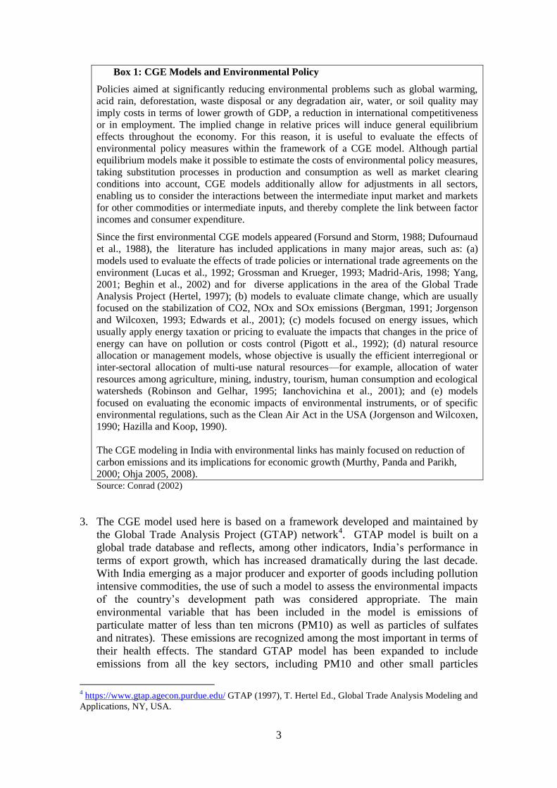
13. As noted above the model was run for the Business as Usual Scenario, plus six

scenarios reflecting a menu of instruments that look at the impacts of reducing

PM10 and other particles through different tax instruments (see Figure 2). Details of

the different scenarios are given in Table 1.

Figure 2: How the CGE Model Works

Two types of taxes are modeled:

Domestic fuel tax (to) is added to the producer price (ps) for coal, oil, natural gas and

refined oil to obtain the market price (pm):

(1) eq. 1

The tax rate increases at a decreasing growth rate starting from 2012. Tax rates (to)

used in different scenarios are displayed in Table 4.

(eq. 2)

Imported fuel tax (tm) is applied to the import price (pms) of coal, oil, natural gas and

refined oil.

Inputs

• Social Accounting Matrix created for India using GTAP data and inouts from various government sources, academic literature

• Estimates on potential emission reduction programs

CGE Model

• Simulate Indian economy under various scenarios covering 57 sectors

Instruments

• Endogenous energy efficiency and end of pipe technology improvements

• Environmental taxes

• Transition to cleaner and cost effective production technologies and processes

Outputs

•GDP

• PM10 Emissions

9

(eq. 3)

(eq. 4)

The tax rate on imported fuel also increases linearly at a constant rate starting

from 2012. Tax rates used in different scenarios are given in Table 4.

Business as Usual (BAU) GDP Growth Scenario

14. The (BAU) GDP growth scenario refers to a purely economic baseline and is based

on past economic performance for 2007–10 and on IMF projections of GDP for

2011–2015, with associated projections up to 2030 derived from projections for

population and TFP. The model then calculates the required investments to achieve

the projected growth, along with the demands for different types of fuel. Domestic

prices for fuel as well as other goods are determined so that demand and supply are

equated. Some emission reduction (and therefore decline in PM intensity of GDP)

happens under BAU due to autonomous technological change built into the model.15

This is partly driven by the macro-economic structural shift away from the

agriculture sector towards knowledge-based industries, greater and easier access to

global knowledge, technology and capital, and the growth impetus provided by the

commercial and services sectors. In addition the shift also reflects the recent policy

initiatives to reduce the sulfur content of diesel in the transport sector, the use of

compressed natural gas for public transport, emissions limiting performance

standards for passenger vehicles, and stricter enforcement of existing environmental

laws.16

15

Autonomous energy efficiency (kg CO2 emitted per unit of GDP in 2000$) improved by 1% per year

between 1980-2008 (WDI) and our BAU reproduces the same trend.

16

New substitution elasticity between capital and energy was introduced into the standard GTAP model

to capture this effect. This is based on the notion that technical progress is entirely embodied in the

design and operating characteristics of new capital plant and equipment. For example, the energy saving

effects of embodied technical progress depends critically on the rate at which new investment goods

diffuse into the economy. By introducing substitution between capital and energy in the model, we

mitigate CO2 emissions by 20% (India would have emitted emit 3246 mtons in 2030 but with the

substitution only emits 2631mtons under BAU).

10

Table 1: CGE Model — Scenarios

Scenarios Instruments Assumptions Results

BAU GDP Growth

Economic growth of

approximately 7 % p.a. Some PM emission

reduction because of

increase in autonomous

energy efficiency of

supply and end-use

technologies (driven by

current policies).

Green Growth

Using a tax on coal

only. Tax applied to

both domestic and

imported coal.

Tax induced shift to a

greener fuel mix and

annual energy efficiency

gains over and above the

historic trend. Limited

investment availability and

turnover of capital stock.

A 10 percent reduction in

PM10 and other small

particles in 2030 over and

above reductions achieved

under BAU Using a tax on PM10.

Tax applied to coal

and oil in relation to

the emissions of PM10

and other small

particles

Green Growth Plus

Using a tax on coal

only. Tax applied to

both domestic and

imported coal.

Tax induced shift leading

to significant improvement

in coal technologies along

with change in plant

vintages over time. Higher

investment availability and

faster turnover of capital

stock.

A 30 percent reduction in

PM10 and other small

particles in 2030 over and

above reductions achieved

under BAU Using a tax on PM10.

Tax applied to coal

and oil in relation to

the emissions of PM10

and other small

particles.

Green Growth scenario

15. The Green Growth Scenario targets a reduction in PM10 and other small emissions

by 10 percent more that what could be achieved relative to BAU in 2030. The

Green Growth Scenario is thus a modified version of the BAU GDP Growth

Scenario, where a tax instrument is used to achieve a targeted emissions reduction.

This is modeled through a tax on coal or through a tax on PM10.17

A tax thus

17

Although most countries use technical standards to curb air pollutants, modeling the effect of market-

based instruments is useful because they favor allocation through relative prices. This is consistent with

India‘s recent approach to use market based instruments to deal with air pollution. The Government of

India introduced on July 1, 2010 a nationwide coal tax of 50 rupees per metric ton ($1.07/t) of coal both

produced and imported into India. The tax raised 25 billion rupees ($535 million) for the financial year

2010–2011. Many consider this coal tax is a step towards helping India meet its voluntary target to reduce

the amount of carbon dioxide released per unit of gross domestic product by 25% from 2005 levels by

2020. Further, India's federal cabinet on April 12, 2012 approved a proposal to change the method used to

calculate the royalty that coal miners pay to state governments, imposing a flat 14% tax based on prices.

11

designed on polluting inputs will raise the unit cost of production and, responding to

the rise in unit cost of production, 18

the producer will reduce the output or substitute

it with a more eco-friendly input. Either of these actions will reduce pollution. It is

thus anticipated that the tax in the model will encourage a shift to a greener fuel mix

and annual energy efficiency gains over and above the historic trend. In the case of

a tax on PM10 for instance we consider a modest tax as a way of reducing particle

emissions per unit of coal used. For further reductions in PM the tax has to induce a

shift out of coal to cleaner fuel. The scenario outline is summarized in Table 1.

Green Growth Plus Scenario

16. The Green Growth Plus Scenario incorporates a more aggressive target of a 30

percent reduction in PM10 and other small particles in the air in 2030 over what

could be achieved under the BAU. Here again, targeted small particles emissions

reduction is attained through a tax on coal or through a tax on PM10.

17. One important difference between the Green Growth and Green Growth Plus

scenarios is that the latter assumes that, as the economy matures, the market realizes

the economic benefits of cleaner and more efficient production. Gradually the

environmental command-and-control ‗push‘ policies in the initial periods are

replaced in the medium to long run by market-driven pull policies to achieve

cleaner and more efficient production. For example, the performance of coal

technologies improves over time, reflected in their rising plant load factor, and

newer plant vintages, with more of the older, less efficient plants getting replaced

and in the increased penetration of advanced coal technologies like super-critical

pulverized coal and integrated gasification combined cycle which will become

competitive over time. While recognizing the limitations of incorporating all these

technologies within the CGE framework, they have been modeled through broad

alterations in investments and emission coefficients. The idea is that the latest

vintage, added to aggregate capital stock, embodies innovation and technological

improvement with no additional cost to the producer.19

18. The CGE model used in this analysis was limited in terms of formulating different

policy scenarios because the current dataset included only five types of energy

sources-- coal, crude oil, refined oil and coal products, natural gas and electricity.

Based on data availability, the model and study can be expanded in the future to

include other energy sources, such as renewable energy and carbon sequestration

measures.

Calibrating the Model for the BAU GDP Growth Scenario

19. Estimates of growth in population and labor force were based on projections made

by national / international sources (e.g. the National Council for Applied Economic

Research (NCAER), UN and World Bank). Medium projections were used for

measuring population growth in 2007-2030 using UN demographic data. The annual

18

Environmental taxes are corrective measures for dealing with the environmental "externality" first

studied by Pigou (1932). A Pigouvian approach sets taxes equal to the marginal damage caused to the

environment by the production process thereby "internalizing" the full social marginal costs.

19

A more formal representation of this can be found in Conrad and Henseler-Under (1986).

12

TFP growth (which picks up the exogenous factors that influence growth in an

economy) was assumed to be 2 percent a year. This is somewhat conservative but

not out of line with previous studies for India. The NCAER CGE model assumes

TFP growth of 3% p.a., as do the Energy and Research Institute (TERI) MOEF

Model and the IRADE AA Model. However the same studies cite others that

assume figures of between 1 and 3 percent. Given this range an assumed value of 2

percent seems reasonable.

20. The assumed annual growth rate in real GDP from 2010 to 2030 is estimated at 6.7

percent. The economic growth (measured as an index) rises from 100 in 2010 to 367

in 2030. This is the Conventional GDP Growth (BAU) scenario estimate (as per

NCAER and recent IMF projections) without correcting for implication of any new

policy changes to deal with pollution..

21. The standard GTAP model‘s structure has been modified to allow substitution

between capital and energy (by increasing the elasticity of substitution from 0 to 0.5,

as in the GTAP-E model). This modified version of the model is close to the energy

version of the GTAP model (called GTAP-E) but does not comprise a nested

structure in the energy block (which would require more data than was available).

Method for estimating PM10 emissions

22. The demands for different kinds of energy and the outputs of the different sectors

were converted to PM10 emissions using corresponding emission coefficients (α(i,j)

and Βi, respectively).20

The Conventional GDP Growth scenario (BAU) generated

PM10 emission estimates for 2010–2030 from fuel use and production activities as

described in equation (1) below:

(Eq. 5)

E = PM10 emissions

Ci,j = Demand for fuel products j in Sector i

i = Sector (firm, household, government)

j = Energy (coal, crude oil, refined oil and coal products, natural gas, and

electricity).

αi,j = Emission coefficient associated with the consumption of one unit of

energy product j by the Sector i

XPi = Production activity and process of sector i

βi = Emission coefficient associated with one unit of output in sector i.

23. Both the consumer demand for energy products (Ci,j) and sectoral economic activity

(XPi) up to 2030 were estimated by the CGE model.

24. First, PM10 emission coefficients are taken from the Garbaccio et al. (2000) study

for China. This is presently the only source for these coefficients being mapped

20

Emission coefficients vary through time to reflect technological change, modernization of power plants,

improved energy efficiency and India‘s emission abatement levels (on the basis of 1% annual increase on

average in BAU reported in WDI statistics).

13

across sectors to the CGE model based on the GTAP database.. The Institute for

Applied System Analysis (IIASA) reports PM10 and other secondary emissions for

India, which corresponded to almost to 8.7 million tons in 2010. The emission

coefficients based on Garbaccio et al. (2000) were updated to reproduce the

aggregate PM10 and other small particles level for India in 2005 and then

extrapolated following the growth assumptions in BAU.

25. Table 3 in Annex 1 represents the relative shares of PM10 emissions by sector and

energy (αi,j).

26. Emissions from productive activities and the respective coefficients (βi) were

calculated as follows:

First, the shares of production activities and process (XP) and energy use (C)

related emissions in total emissions (E) were calculated as per the Garbaccio et

al. (2000) study. Second, sector-specific emission coefficients in Garbaccio et al. (2000) were re-

adjusted according to the GTAP classification in proportion to the sector‘s

contribution to overall PM10 emissions and overall emission estimates from the

IIASA model.

27. On the basis of equation (1) and the CGE simulations, the increase in PM10

emissions and other particulate emissions over time was calculated as a function of

the demand for each type of energy by sectors (Ci,j), and the economic expansion of

production activities (XPi).

28. Second, the emissions coefficients αij and βi are modified over time to account for

the improvements in the emission-capturing technologies, ; through (a) a shift to

cleaner coal (imported coal has lower emissions per unit of energy than domestic

coal and its share in the total amount of coal used in India is rising); and (b) other

measures such as coal washing. These reductions in emissions are partly driven by

administrative measures, and partly by trade factors and such improvements are

included in the BAU. The rates of decline in unit emission are for these reasons

taken from micro studies (see Cropper et al, 2012). Further reductions in the

coefficients may be achieved through a tax on PM10 and similar emissions. Such

reductions in the coefficients reflect the impact of further pollution control measures

that will be introduced as a result of the tax.21

29. The energy demand in value (US$) for four fuel types — coal, crude oil, oil and coal

products, and natural gas — were obtained for 2010–2030 using the CGE model.

This was converted into volume in terms of Thousand Tons of Oil Equivalent

(TTOE) using appropriate factors.

Main Results

PM10 and other particle emissions

30. Fossil fuel use, the primary cause of pollution, is expected to decrease under BAU

due to a declining share of coal in the overall energy demand (although coal would

still dominate in 2030); to greater emissions capture; and to the shift to cleaner coal.

Demand for refined oil products and electricity, however, will still increase

considerably. As a result, the share of emissions from productive activities in total

21

The PM10/CO2 elasticity varies across scenarios, the average is found to be 1.62 which means that 1

unit of CO2 abatement will bring 1.62 unit of PM10 abatement.

14

PM10 emissions is expected to double along with the impacts of the fast-increasing

economic activities, such as manufacturing and construction, and transportation.

The total PM10 emissions under BAU are estimated to go up from 8.7 million tons

in 2010 to 16.8 million tons in 2030, an annual rate of increase of 1.9 percent

against an annual GDP increase of 6.7 percent (Figure 3). Emission will grow more

slowly than GDP because of the exogenous factors noted above.

Figure 3: Total PM10 and Similar emissions (BAU GDP Growth scenario) (in million

tons)

Conventional GDP Growth scenario vs. Green Growth Scenarios

31. Recall that the Green Growth Scenarios seeks to constrain particulate emissions

through a menu of instruments that translate into 10 percent or 30 percent less than

emissions under the BAU scenario. They do this by imposing different fuel or

emission taxes, as already described, along with other assumed reductions in

emissions resulting from low-cost measures especially in the Green Growth plus

scenario which are encouraged by tax policies that operate outside the scope of the

model. The combined effect of the two drivers – the tax measures, and the other

low-hanging fruit measures –results in reduction in emissions of PM and CO2.

Table 2 shows the following results:

Table 2: Comparing the Base Case (BAU) with a 10% and 30% Reduction in PM

15

2010 2030 Percentage

Increase

p.a.

GDP

loss %

wrt BAU

%

reduction

in CO2

wrt BAU

BAU

GDP US$Bn.

2010

3,763 13,820 6.89

CO2: Mn. Tons 1,563 2,770 1.77

PM10: Mn. Tons 8.68 16.81 1.94

10% Reduction Via a PM tax 20%

GDP US$Bn.

2010

3,763 13,774 6.87

0.33

CO2: Mn. Tons 1,563 2,180 0.79

PM10: Mn. Tons 8.68 15.12 1.03

10% Reduction Via a Coal Tax 10%

GDP US$Bn.

2010

3,763 13,751 6.86

0.5

CO2: Mn. Tons 1,563 2,499 0.9

PM10: Mn. Tons 8.68 15.24 1.03

30% Reduction Via PM Tax

60%

GDP US$Bn.

2010

3,763 13,723 6.85

0.7

CO2: Mn. Tons 1,563 1,108 0.4

PM10: Mn. Tons 8.68 11.86 1.02

30% Reduction Via Coal Tax 30%

GDP US$Bn.

2010

3,763 13,672 6.83

1.07

CO2: Mn. Tons 1,563 1,939 0.7

PM10: Mn. Tons 8.68 11.84 1.02

The results in summary are:

i. With the different tax regimes for a 10 percent particulate emission reduction

we have a lower GDP but the size of the reduction is modest. With a PM10

tax conventional GDP is about US$46 billion lower in 2030, representing a

loss in growth of 0.3 percent with respect to BAU. The impact on GDP is

greatest if we seek to achieve the PM target via a coal tax.

ii. For a 30 percent particulate emission reduction the conventional GDP is

about US$97 billion lower in 2030 representing a loss of 0.7 percent. The

scenario suggests that even a substantial reduction in emissions can be

achieved without compromising much on GDP growth rates if supported by

adequate least cost policy measures. Again the coal tax performs worse with

a GDP loss of 1.07 percent.

iii. It should also be noted that the Green Growth Plus scenario assumes, in

addition to the taxes, some increase in investment towards cleaner

technologies. Such investments are associated with an increase in pollution

control techniques, modernization of the existing capital and/or use of less

16

polluting capital over time with very low additional cost to the producer (see

Box 3). These outside-the-model emission declines are assumed to be

stimulated by the new investments, but themselves having minimal

economic costs--play a crucial role in the analysis of the environment-

growth tradeoffs for this scenario. They account for almost two-thirds of the

PM10 reductions (20 out of 30percent) in the Green Growth Plus Scenario.

If we do not include these minimal-cost emissions savings from outside the

model, there would be bigger negative GDP impacts indicated by

adjustments of inputs and outputs in the model. We would, however, argue

that the stronger tax regime will result in enterprises looking for to realize

benefit from these low-cost mitigation measures.22

iv. On the welfare side, health damages from PM are significantly reduced in

the 30 percent reduction case when compared to a 10 percent reduction

(Table 3). Savings range from U$24 billion from reduced health damages in

the case of a 10 percent reduction (lower estimate) to US$105 billion in the

case of a 30 percent reduction (upper estimate scenario). The central

estimates are in US$34-$67 billion range which more or less offsets the GDP

loss from the introduction of the tax. The introduction of tax regimes lowers

GDP in all scenarios but this can be at least partially offset by the benefits of

lower health damages.

v. The different tax regimes provide an important co-benefit in terms of

substantial reduction in CO2 emissions. We find the PM tax makes the

bigger reduction in these emissions than the coal tax. Our calculations show

that even with a value per ton of CO2 of just US$10 the reduction in CO2

for the 10 percent PM reduction case is worth US$59 billion which is little

more than the loss of GDP. For the 30 percent reduction case the reduction is

worth US$83 billion, slightly less than the loss of GDP. In addition we can

take account of the savings in PM10 damages too which gives an overall net

gain through this route (see Table 3).

vi. Also, Given our assumptions on economy and environmental targets in

2030, the model gave us the percent of tax we have to apply on coal (first

scenario) and coal/oil (second scenario) (see Table IV). We shocked the

energy in BAU by these tax rates to reach our PM10 reduction targets.

vii. In terms of sector prices, we find that the energy-intensive sectors will be the

most impacted in 2030 under the various tax regimes. While the electricity,

petroleum, chemical and minerals sectors will be impacted the most from a

PM tax, metal products (e.g. iron and steel) will be most affected from a coal

tax.

22

As a result of tax policies private firms are expected to invest in clean technologies: either financed by

FDI or through domestic investments. This investment may even generate new activity sectors if

environment friendly technologies are domestically produced. According to the model estimations these

new investments will generate a value added equivalent of 0.8-1.2% of GDP in different scenarios that we

simulated.

17

Box 3: Technologies for Control of PM10 and CO2 from Power Plants in India

Control of particulate emissions from power plants has been a concern in India for many years

now, especially because of the high ash content of Indian coal which is the primary fuel for the

overwhelming majority of thermal power plants. Over the last two decades, various studies have

been carried out to establish effective ways of dealing with these emissions over time (Lookman

and Rubin (1998), Kumar and Rao (2002), TERI (2003), Murthy et.al. (2006), Sengupta (2007),

Cropper et. al. (2012)).

Coal beneficiation is the process of removal of the contaminants and the lower grade coal to

achieve a product quality which is suitable to the application of the end user - either as an

energy source or as a chemical agent or feedstock.

A common term for this process is coal "washing" or "cleaning". According to Zamuda and

Sharpe (2007), Indian coals are of poor quality and often contain 30-50% ash when shipped to

power stations. In addition, over time the calorific value and the ash content of thermal coals in

India have deteriorated as the better quality coal reserves have been depleted and surface mining

and mechanization expanded. This poses significant challenges. Transporting large amounts of

ash-forming minerals wastes energy and creates shortages of rail cars and port facilities. Coal

washing reduces the ash content of coal, improves its heating value and also removes small

amounts of other substances, such as sulfur and hazardous air pollutants. The benefits of using

washed coal, inter alia, include reductions in particulate and sulfur emissions, reductions in

flyash disposal costs and reductions in the cost of transporting coal, per unit of heat input. Use

of washed coal may also reduce plant maintenance costs and increase plant availability.

Installing a washery for coal would entail an expenditure of around INR 400 million for a 3

MTPA plant. According to Zamuda and Sharpe (2007) for a typical 500 MW plant, the use of

washed coal with ash reduced from 38% to 30% could result in a 2% reduction in the cost of

electricity generation with savings averaging INR 0.035 per kWh of generated power, once

various benefits to plant operation and reduced emissions are accounted for. Lookman and

Rubin (1998) had previously analyzed 174 plants across India and found that coal cleaning

could result in savings in the range of of USD75-150 million and USD15-25 million for

existing plants by 2002 in terms of 1996 dollars. More recently, Cropper et. al. have, using

updated figures from India‘s Central Electricity Authority for a particular plant in Rihand,

estimated that levelized cost of electricity generation increases from INR 1.206 to INR 1.405

but did not take into account any of the other benefits that Zamuda and Sharpe quantified.

Table 3: Health Damage Estimates for Alternative Scenarios

2010 2030 2030 2030

Morbidity (US$Bn.) BAU

10% PM

Reduction

30% PM

Reduction

Lower 32.38 230.46 206.94 160.96

Central 46.12 328.37 294.84 229.28

Upper 72.39 515.24 462.64 359.83

Mortality (US$Bn.)

Lower 9.31 14.02 13.56 12.47

Central 14.87 22.36 21.63 19.90

Upper 20.39 30.65 29.65 27.29

18

Total (US$Bn.)

Lower 41.70 244.49 220.50 173.43

Central 60.99 350.73 316.48 249.18

Upper 92.78 545.90 492.29 387.11

Saving (US$Bn.) from Reduced

Health Damages

Lower 23.99 47.07

Central 34.25 67.30

Upper 53.60 105.18

Table 4: Different Taxes (%) for a 10% Reduction in PM Emissions by 2030 -- derived from the

CGE simulations

Tax Regime

Applied to 2014 2030

Coal Tax

Coal 14.0% 38.5%

PM Tax

Coal, Oil 3.4% 16.2%

Conclusions

33. The study shows that policy interventions such as environmental taxes are likely to

yield positive net environmental benefits for India. The CGE analysis also shows

that addressing "public bads" via selected policy instruments need not translate into

large losses on GDP growth. The environmental cost model developed in this study

can thus be used to evaluate the benefits of similar pollution-control policies and

assist in designing and selecting appropriate targeted intervention policies (such as a

SO2 tax, a CO2 tax, or emission trading schemes). Once the impact on ambient air

quality of a policy to reduce particulate emissions is estimated, the tools used to

calculate the health damages associated with particulate emissions can also be used

to compute the welfare impacts of reducing them. The monetized value of the health

benefits associated with each measure can be calculated, using the techniques

developed in this study, and compared with the costs.

36. The comparisons made between the BAU scenario and the Green Growth scenarios

reveal that a low carbon, resource-efficient, greening of the economy should be

possible at a very low cost in terms of GDP growth. This would make the Green

Growth scenarios attractive compared to the Conventional GDP Growth scenario. A

more aggressive low carbon strategy (Green Growth Plus) comes at a slightly higher

price tag for the economy while delivering higher benefits. The extent to which

GDP growth would be impacted under more severe cuts on polluting emissions has

to be determined by further study using the CGE model. On the other hand, the

modest GDP impacts indicated in this study depend on the availability of minimal-

cost mitigation options (energy efficiency improvements, embodied technological

improvements, improved daily operating practices of boilers). With fewer such

options, the GDP cost of hitting the 10 percent and 30 percent targets would be

19

higher – potentially considerably higher. In evaluating the environment-growth

tradeoffs, accordingly, a judgment must be made about the size and availability of

such ―low hanging fruit‖ and appropriate incentives.

37. Both Green Growth scenarios have other important benefits. Most significantly

they reduce CO2 emissions, which have an important value. If we take that value at

even a modest US$10 per ton, reflecting what might be gained in revenues from

participation in emerging carbon abatement markets, India could realize an

additional benefit of around US$59 billion (with a PM10 tax). Global carbon

models estimate that these emissions could be worth much more—US$50-120—by

2030. The green growth scenarios have other environmental benefits we have not

included, especially in the areas of natural capital [elaborated in the companion

paper, ―Valuation of Biodiversity and Ecosystem Services.‖]. Finally the Green

Growth scenarios produce benefits for all: i.e. they have distributional advantage

over the conventional scenario.23

38. The findings and conclusions of this study and the use of the CGE model should

also be considered in the context of various assumptions/limitations.

Only particulate emissions were analyzed; other local environmental issues

were not considered.

The baseline PM10 and other particulate emissions used in the CGE model

were obtained from the IIASA literature on India and were not based on actual

measurements.

The CGE model did not separate health services from overall public services

as an economic sector. The expected expansion of health services to address

the increasing environmental health issues was not separately covered.24

The CGE model has a medium- to long-term structure and therefore could not

cover short-term fluctuations, e.g. oil price volatility.

Both production sectors (57) that cover agriculture, manufacturing, services,

and households were represented as prototypes; thus the distributional

environmental health impacts on different economic strata and geographic

locations were not taken into account.

39. The study shows that the CGE model could be used as a tool for policy making.

Being a general equilibrium open economy model, its strengths lie in the

representation of inter-sectoral linkages both within and outside the country. At an

economy-wide level, the CGE model makes it possible to determine whether growth

objectives are compatible with the environmental objectives. The management of

pollutants at the sectoral level can also be used to determine the abatement costs

across the sectors. Distributional implications (winners vs. losers) among the sectors

could also be analyzed.

40. Further work using the CGE model after correcting for environmental health

impacts would be useful in policy making. The present approach has the flexibility

to incorporate multiple scenarios, e.g. the various scenarios in Parikh (2009) to

23

Improving air quality is a public good. Even if poor air quality affects all equally, an improvement has

a bigger proportional benefit to the poor. And there is evidence that the poor are more affected by air

pollution.

24

Health services are in the same category as education and defense: public services. They are separated

from other services provided by the private sector such as trade, transport etc

20

determine the implications on GDP, which could be further corrected for

environmental health impacts. The CGE approach described in this study was fairly

detailed, with the 57 sectors tailored to India-specific parameters. The study

recommends the use of this approach for the following possible scenarios:

Including more energy sources so that it explicitly accounts for more renewable

and nuclear energy.

Considering higher levels of de-carbonization and carbon capture and storage

(CCS) as targets to be modeled and evaluated against the Conventional GDP

Growth scenario.

Examining different instruments (beyond the ones examined here) to achieve

the shift from the Conventional GDP Growth scenario to an environmentally

sustainable scenario.

21

References

ADB, GEF, UNDP (1998): Asia Least Cost Greenhouse Gas Abatement Strategy:

ALGAS India, Manila, Philippines.

Beghin, J., Dessus S., Roland-Holst, D., Van der Mensbrugghe, D.(1996). General

Equilibrium Modeling of Trade and the Environment, Technical Paper, N8 116, Paris,

OECD Development Center.

Beghin, J., Bowland, B., Dessus, S., Roland-Holst, D., Van der Mensbrugghe, D.,

(2002). Trade integration, environmental degradation and public health in Chile:

assessing the linkages. Environment and Development Economics 7 (2), 241– 267.

Bergman, Lars, (1991). General equilibrium effect of environmental policy: a CGE

modeling approach. Environmental and Resource Economics 1, 43– 61.

Bhalla, Surjit (2007): Second Among Equals: The Middle Class Kingdoms of India and

China (forthcoming), Institute of International Economics, Washington D.C.

Bovebourg A.L. and L.H. Goulder (1996). Optimal Environmental Taxation in the

Presence of Other Taxes: General-Equilibrium Analyses, American Economic Review

86(4):985-1000.

Burniaux, J. M. and T.P. Truong (2002), GTAP-E: An Energy Environmental Version

of the GTAP model with Emissions, Centre for Global Trade Analysis, Technical paper

16.

Bussolo, M. and O‘Connor, D. (2001). ―Clearing the Air in India: The Economics of

Climate Policy with Ancilliary Benefits,‖ Development Centre Working Paper 182,

CD/DOC 14, OECD.

Central Pollution Control Board (2006). Air Quality Trends and Action Plan for Control

of Air Pollution from Seventeen Cities. Available at

http://www.cpcb.nic.in/upload/NewItems/NewItem_104_airquality17cities-package-

.pdf, (last accessed 24 January, 2011).

Central Pollution Control Board (2009). Ambient Air Quality Standards. Available at

http://cpcbenvis.nic.in/airpollution/standard.htm (last accessed 24 January, 2011).

Central Pollution Control Board (2009). Comprehensive Environmental Assessment of

Industrial Clusters. Available at

http://www.cpcb.nic.in/upload/NewItems/NewItem_152_Final-Book_2.pdf (last

accessed 19 June, 2011).

Central Pollution Control Board (2010). National Air Quality Monitoring Program.

Available at http://cpcbenvis.nic.in/airpollution/finding.htm (last accessed 24 January,

2011).

22

Central Pollution Control Board (2011). Air Quality Monitoring, Emission Inventory

and Source Apportionment Study for Indian Cities: National Summary Report.

Available at http://cpcb.nic.in/FinalNationalSummary.pdf.

Central Pollution Control Board, Environmental Data Bank: RSPM Emission Data by

city obtained during the period from March 2009 to June 2009. www.cpcbedb.nic.in

Conrad, K. and I. Henseler-Unger (1986). ―Applied General Equilibrium Modeling for

Longterm Energy Policy in the Fed. Rep. of Germany,‖ Journal of Policy Modeling, 8

(4), 531-49.

Cropper, M., S. Gamkhar, K. Malik, A. Limonov, and I. Partridge (2012): Air Pollution

Control in India: Getting the Prices Right; available at

www.aeaweb.org/aea/2012conference/program/retrieve.php?pdfid=600

Cropper, M. L., Nathalie, B. S., Anna, A. Seema, A., Sharma, P. K. (1997). ―The Health

Benefits of Air Pollution Control in Delhi‖, American Journal of Agricultural

Economics, Vol. 79, No. 5, Proceedings Issue, 1625-1629.

Dufournaud, M., Harrington, J., Rogers, P., (1988). Leontief‘s environmental

repercussions and the economic structure revisited: a general equilibrium formulation.

Geographical Analysis 20 (4), 318– 327.

Edwards, T. Huw, Hutton, John P., (2001). Allocation of carbon permits within a

country: a general equilibrium analysis of the United Kingdom. Energy Economics 23

(4), 371–386.

Forsund, F., Storm, S., (1988). Environmental economics and management: pollution

and natural resources. Croom Helm Press, New York.

Greenstone, M., A. Krishnan, N.Ryan and A.Sudarshan (2012). ―Improving Human

Health Through a Market-Friendly Emissions Scheme,‖ Seminar Volume for

International Seminar on Global Environment and Disaster Management: Law and

Society (organized by Supreme Court of India, Ministry of Environment and Forest and

Law Ministry).

Gosain, Rao and Basuray (2006). ‗Climate change impact assessment on hydrology of

Indian river basins,‘ Current Science, Vol. 90, No. 3, February.

Goulder, L., ed. (2002). Environmental Policy Making in Economics With Prior Tax

Distortions, Northampton MA: Edward Elgar.

Greenstone, M., A. Krishnan, N.Ryan and A.Sudarshan (2012). ―Improving Human

Health Through a Market-Friendly Emissions Scheme,‖ Seminar Volume for

International Seminar on Global Environment and Disaster Management: Law and

Society (organized by Supreme Court of India, Ministry of Environment and Forest and

Law Ministry).

23

Grossman, G., Krueger, A., (1993). Environmental impacts of a North American free

trade agreement. In: Peter, Garber (Ed.), The Mexico–US Free Trade Agreement. The

MIT Press, Cambridge.

Gunning, J.W. and M. Keyzer (1995). Applied General Equilibrium Models for Policy

Analysis, in J. Behrman and T.N. Srinivasan (eds.) Handbook of Development

Economics Vol. III-A, Amsterdam: Elsevier, 2025-2107

Guttikunda S. and Jawahar P. (2011): Urban Air Pollution & Co-benefits Analysis in

India – for Climate Works Foundation and Shakti Foundation - shared by Author

Hertel, Thomas et al. (1997), Global Trade Analysis Modeling and Applications, T.

Hertel Ed, NY, USA.

Kumar, Surender and Rao, D.N. (2003) "Estimating Marginal Abatement Costs of SPM:

An Applicaiton to the Thermal Power Sector in India," Energy Studies Review: Vol. 11:

Iss. 1, Article 2. Available at: http://digitalcommons.mcmaster.ca/esr/vol11/iss1/2

Hazilla, M., Koop, R., (1990). Social cost of environmental quality regulations: a

general equilibrium analysis. Journal of Policy Modeling 98 (4), 853– 873.

Ianchovichina, Darwin, E.R., Shoemaker, R., (2001). Resource use and technological

progress in agriculture: a dynamic general equilibrium analysis. Ecological Economics

38, 275– 291.

International Monetary Fund (2012). India: 2012 Article IV Consultation-Staff Report.

International Monetary Fund (2011). World Economic Outlook: Slowing Growth,

Rising Risks, September 2011, IMF: Washington, DC.

Jorgenson, D.W., Wilcoxen, P., (1990). Intertemporal general equilibrium modeling of

U.S. environmental regulation. Journal of Policy Modeling 12 (4), 715– 744.

Jorgenson, D.W., Wilcoxen, P., (1993). Reducing U.S. carbon dioxide emissions: an

assessment of different instruments. Journal of Policy Modeling 15 (5), 491– 520.

Kumar, Surender and Rao, D.N. (2003) "Estimating Marginal Abatement Costs of SPM:

An Applicaiton to the Thermal Power Sector in India," Energy Studies Review: Vol. 11:

Iss. 1, Article 2. Available at: http://digitalcommons.mcmaster.ca/esr/vol11/iss1/2

Lookman A. and Rubin E. S. (1998). Barriers to adopting least-cost particulate control

strategies for Indian power plants; Energy Policy Vol. 26, No. 14, pp 1053-1063.

Elservier Science Ltd.

Lucas, R., Wheeler, D., Hettige, H., (1992). Economic development, environmental

regulation and the international migration of toxic industrial pollution: 1960–1988. In:

Patrick, Low (Ed.),

International trade and the environment, World Bank Discussion Paper, vol. 159, pp.

67–88. Washington, DC.

24

Madheswaran, S. (2007). ―Measuring the value of statistical life: estimating

compensating wage differentials among workers in India.‖ Social Indicators Research,

84(1).

Madrid-Aris, M.E., (1998). International trade and the environment: evidence from the

North America Free Trade Agreement(NAFTA). Presented in the World Congress of

Environmental and Resources Economics, Venice, Italy, June 25–27.

Markandya, A. (2006). ―Water Quality Issues in Developing Countries‖, in ‖ in R.

Lopez and M. A. Toman (eds.) Economic Development and Environmental

Sustainability, Columbia University Press.

Martin,W. and L.A. Winters, eds. (1996). The Uruguay Round and the Developing

Economies, New York: Cambridge University Press

McDougall, Robert (2007), GTAP-E 6 pre-2,

https://www.gtap.agecon.purdue.edu/resources/res_display.asp?RecordID=2957

Ministry of Environment and Forests (2009). State of Environment Report. Available at

http://envfor.nic.in/soer/2009/SoE%20Report_2009.pdf

Ministry of Environment and Forests (2010): Report to the People on Environment and

Forests 2009—2010, Government of India, New Delhi.

Ministry of Statistics and Programme Implementation, Government of India, National

Sample Survey Organization, ―Some Characteristics of Urban Slums July 2008 – June

2009,‖ NSS 65th

Round, May 2010.

MIT (2004). Computable General Equilibrium Models and Their Use in Economy-Wide

Policy Analysis, Technical Note No. 6, September 2004.

Murty, M.N. ; Kumar, Surender and Dhavala, Kishore (2006): Measuring

Environmental Efficiency of Industry: A Case Study of Thermal Power Generation in

India; MPRA paper no. 1693; Online at http://mpra.ub.uni-muenchen.de/1693/

Ojha, V. P. (2005). ‗The Trade-off Among Carbon Emissions, Economic Growth and

Poverty Reduction in India,‘ SANDEE Working Paper No. 12-05, South Asian Network

for Development and Environmental Economics, Nepal, August.

Ojha, V. P. (2008): "Carbon emissions reduction strategies and poverty alleviation in

India", Environment and Development Economics, No: 14: 323-348

Ostro, B. (1994). ―Estimating the Health Effects of Air Pollutants: A Method with an

Application to Jakarta.‖ The World Bank, Policy Research Working Paper, 1301.

Ostro B. (2004). Outdoor air pollution: Assessing the environmental burden of disease

at national and local levels. Geneva, World Health Organization, (WHO Environmental

Burden of Disease Series, No. 5).

Panagariya, Arvind (2008). ‗India: The Emerging Giant,‘ Oxford University Press.

25

Parikh, K. (2009), ‗India‘s Energy Needs, CO2 Emissions and Low Carbon Options‘,

22nd International Conference on Efficiency, Cost, Optimization, and Environmental

Impact of Energy Systems, August 31 – September 3, 2009, Foz do Iguaçu, Paraná,

Brazil

Perry, G., J. Whalley and G. McMahon, eds. (2001). Fiscal Reform and Structural

Change in Developing Countries, New-York: Palgrave-Macmillan.

Pigott, J., Whalley, J., Wigle, J., (1992). International linkages and carbon reduction

initiatives. In: Anderson, K., Blackhurst, R. (Eds.), The greening of world trade issues.

University of Michigan Press.

Pigou, A. (1932): The Economics of Welfare, MacMillan, London

Robinson, S., Gelhar, C., (1995). Land, water and agriculture in Egypt: the economy-

wide impact of policy reform. Discussion paper. International Food Policy Research

Institute, Washington, DC.

Rodrik, Dani and Arvind Subramanian (2004): ‗Why India Can Grow at 7 % a Year or

More‘, Economic and Political Weekly, April 17.

Sengupta I. (2007): Optimal time for investment to regulate emissions of particulate

matter in Indian thermal power plants, Environment and Development Economics 12:

827-860, Cambridge University Press

Shanmugam K.R. (1997). ―The Value of Life: Estimates From Indian Labour Market‖

The Indian Economic Journal, 105 – 114.

Shields, C.R. and J.F. Francois, eds. (1994). Modeling Trade Policy: Applied General

Equilibrium Assessments of North American Free Trade, New York: Cambridge

University Press.

TERI (2003): Electricity externalities in India: information gaps and research agenda;

The Energy and Resources Institute, New Delhi

United Nations, Deprtment of Economic and Social Affairs, Population Division, World

Urbanization Prospects, 2009.

Vital Statistics Division, Registrar General India, ―Sample Registration System

Bulletin,‖ October 2009.

Wilson, Dominic and Roopa Purushothaman (2003). ‗Dreaming with BRICS: The Path

to 2050,‘ Global Economics Paper No.99, Goldman Sachs

World Health Organization (2008). Air Quality and Health. Available at

http://www.who.int/mediacentre/factsheets/fs313/en/ (last accessed 24 January, 2011).

Yang, Hao-Yen, (2001). Trade liberalization and pollution: a general equilibrium

analysis of carbon dioxide emissions in Taiwan. Economic Modelling 18, 435–

454.Annex 1: Description of the CGE Model

26

27

I. The economic growth baseline: GTAP-India 2030 model

Definitions; Computable refers to numerically solvable models. General refers to an

economy-wide approach. Equilibrium is satisfied at multiple levels between (i) demand

and supply of factor of production, commodities, and services, (ii) consumers‘ demands

and their budget constraints (expenses equal revenues), and (iii) macro-economic

balance25

[GDP = C + G + I + (X-M)].

The GTAP model, like most of the standard CGE models, comprises non-linear

behavioral equations and macro-economic accounting links (linear relations describing

the break-even points in different markets).

The model is solved under GEMPACK (General Equilibrium Model Package) which

uses a Euler algorithm; 3-4-5 step extrapolation method.

The Indian economy is modeled as an open economy composed of 57 firms, one

representative household, and the government. Five factors of production exist; skilled

labor, unskilled labor, capital, land, and natural resources.

Commodities/services, capital and labor are mobile across sectors and countries

(international migration is not specified in the current version). The model represents

the circular flow of goods and services in the economy and (i) permits flexibility in

economic agents‘ behaviors, (ii) captures substitution/complementarity relations across

demand for goods and services, and (iii) calculates price changes resulting from

changing demand and supply conditions.

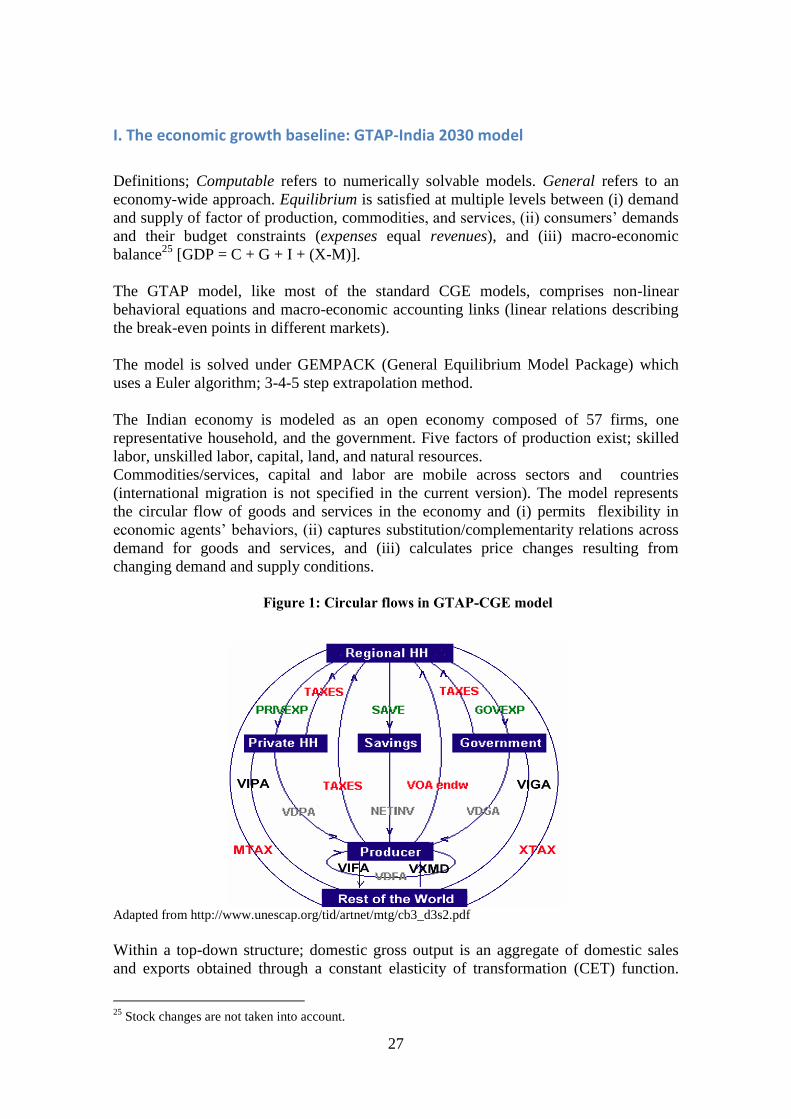
Figure 1: Circular flows in GTAP-CGE model

Adapted from http://www.unescap.org/tid/artnet/mtg/cb3_d3s2.pdf

Within a top-down structure; domestic gross output is an aggregate of domestic sales

and exports obtained through a constant elasticity of transformation (CET) function.

25

Stock changes are not taken into account.

28

The production structure is specified in the form of nested constant elasticity of

substitution (CES) functions that use labor (skilled and unskilled), capital, land and

natural resources as inputs (Figure 2).

Figure 2: Modified production structure of the GTAP-CGE model used in this study

Output / \ / \ <-- [CES] / \ / \ / \ Value Added Intermediate Consumption

| 52 non energy goods <-- [CES] | | /|\ /\ [CES]--> / | \ / \ <-- [Armington] / | \ / \ / | \ / \ / | \ / \ Land Labor Capital - Domestic Foreign

Energy(5)

Intermediate consumption includes 5 energy products; (coal, crude oil, petroleum

products, natural gas, and electricity) and 52 non energy goods. All intermediate goods

are differentiated according to their origin as domestic and imported products. Imports

by the countries of origin follow an Armington specification (1969).

Regional utility per capita is defined at the regional level, within a Cobb-Douglas

function by private consumption, government consumption, and savings.

The demand for final goods is defined at the regional level by (i) household

consumption through a constant-difference-elasticity (CDE) 26

demand specification

which is a non-homothetic demand system; and (ii) public sector using a Cobb-Douglas

aggregation composed of market commodities and government spending where both are

specified as a fixed share of income.

Households' and firms' savings as well as taxes finance investment and government

expenses. The price of utility from private consumption depends on the level of private

consumption expenditure.

26

Elasticities of substitution between pairs of commodities can differ and income elasticities may be

different than one.

29

Figure 3: Consumption module in GTAP-CGE model

Regional per capita utility

(Consumption Expenditure = Income)

/ | \ / | \

/ | \ <--[COBB-DOUGLAS ɣ=1] / | \ / | \ Private household | Government consumption

consumption [CDE] | / \

/ \ | / \ <--[COBB-DOUGLAS ɣ=1] [Armington] | Final \ / \ | Goods Public expenditure / \ | / \ / \ | [Armington] / \ | / \ Domestic Imported Savings Domestic Imported

Goods Goods Goods Goods

The GTAP-India 2030 model is used to develop an economic baseline which represents

the most likely path of development of the Indian economy until 2030. Population/labor

force, capital inflows and productivity growth are the drivers of the economic growth,

no economic policy or pollution control measures are specified.

The economic baseline is developed by applying shocks to the initial equilibrium

conditions that represent the Indian economy and its linkages with the Rest of the World

in 2007.

In order to represent the most likely growth path, the model is solved for successive

years using statistical projections on population, labor supply and TFP, 2 percent per

year following the literature). A new equilibrium: i.e. new prices and demand/supply

conditions are determined for each year.

30

II. The PM10 emission baseline

Fossil fuels are the major source of many local and regional air pollutants including the

suspended particulate matter (SPM) and PM10 emissions. Other sources of particulate

matter include physical processes of grinding, crushing and abrasion of surfaces.

Mining and agricultural activities are also known to contribute larger sized particulate

matter to the environment. In this exercise, the PM10 emissions, which cover the

inhalable size fraction of SPM are estimated in two steps--as input and output related

emissions.

The construction of the environmental baseline captures the influence of the economic

growth drivers on India‘s pollution SPM/PM10 levels. The emission estimates are

introduced into the CGE model to calculate the economy-wide impacts of emission

reduction policies in the last section.

Equation 1 summarizes the PM10 estimation method: (E) emissions comprise input and

output related pollutants. The former refers to fuel combustion related particulate

emissions; therefore it is estimated on the basis of different categories of agents'

demands for fuel (C). The second types of pollutants are emitted during the production

processes (XP) of different sectors.

Eq.

(1)

E = PM10 emissions

Ci,j = Demand for energy products j

i = institution (firm, household, government)

j = energy good (coal, crude oil, natural gas, electricity, refined oil).

αi,j = emission coefficient associated with the consumption of one unit of energy

product j by the institution i

XPi = Output of firm i

βi = emission coefficient associated with one unit of output in sector i.

Most of the CO2 emissions from fuel combustion are directly correlated to the level of

carbon intensive activities, such as electricity generation, production of chemicals and

basic metal products, and consumption of transport fuels; these refer to direct

production-based emissions.

This study borrows inputs from previous studies on India. More specifically, PM10

estimations developed by the International Institute for Applied System Analysis'

(IIASA) GAINS model are used as the initial pollution level in our model. Accordingly,

we assumed that the PM10 emission level corresponded to 7 million tons in 2005.

i

i

ijii j

i j XPβCE α ,

31

Based on the sectoral breakdown displayed in Annex Table 1, we calculated the shares

of PM10 emissions from fuel use in the GTAP model. Approximately 3/4 of PM10

emissions are caused by fuel consumption (5 million out of 7 million tons).

Annex Table 2 shows that 93 percent of the energy consumption at the origin of the

PM10 emissions was domestically produced in 2005. Carbon intensive consumption

accounts for 63 percent of the pollution.

PM10 emissions‘ estimations linked to production process follow the method in

Garbaccio et al. (2000) study for China. They are assumed to represent a certain

percentage of the total PM10 emissions. The corresponding coefficient is borrowed

from the estimations developed by IIASA using the GAINS model. In 2005 output

related PM10 emission represents approximately 26 percent of the total PM10 level27

.

Annex Table 1: PM10 estimations per fuel use (GAINS model simulations -

www.iiasa.ac.at)

27

See Table 3b in Garbaccio et al (2000) study for a list of activities at the origin of PM10 emissions (i.e

construction). However, there is no construction sector in the GTAP model, hence the emissions

coefficient from the Garbaccio et al (2000) are adjusted: "building material", "primary metals", "metal

products" and "construction" sectors have been aggregated into one sector.

1990 1995 2000 2005

PM10 (Thousand tons) 5,702 6,731 7,059 7,032

Brown coal/lignite, grade 1 283 411 360 305

Hard coal, grade 2 1,485 2,023 2,049 2,041

Derived coal (coke, briquettes) 5 4 3 2

Biomass fuels ... 1 0 1

Agricultural residuals - direct use 608 696 802 764

Biogas 0 0 0 0

Dung 814 773 732 590

Fuelwood direct 938 1,020 1,097 1,228

Heavy fuel oil 6 7 8 9

Medium distillates (diesel, light fuel oil) 98 132 180 139

Gasoline and other light fractions of oil

(includes kerosene)

83 117 162 67

Liquefied petroleum gas 1 1 2 3

Natural gas (incl. other gases) 0 0 0 0

Non exhaust PM emissions - road

abrasion

3 3 4 3

Non exhaust PM emissions - brake wear 1 2 2 1

Non exhaust PM emissions - tyre wear 3 4 5 3

No fuel use 1,373 1,536 1,651 1,876

32

Annex Table 2: PM10 emissions per fuel use and origin in GTAP-India 2030 model28

2005 PM10 by fuel

Domestic Imported Total

Coal 3,070,247 216,773 3,287,020

Crude Oil 233 16 250

Natural Gas 259,912 145 260,057

Refined oil& coal products 1,475,492 128,605 1,604,098

Electricity 0 0 0

Total 4,805,884 345,540 5,151,424

Annex Table 3: GTAP mapping of process based emission coefficients

Currently, India‘s major cities have severe air pollution problems, with average ambient

concentrations of pollutants far in excess of WHO guidelines and/or Indian ambient

standards. These problems are expected to increase with the rise of PM10 pollutants and

their adverse effects on human health, which is detailed in the next section.

28

Adapted from Table 1

33

III. Sectoral Sources of Particulate Emissions

Agriculture related

Paddy or rice; wheat; cereal grains and others; vegetables, fruit, nuts; oil seeds; sugar

cane, sugar beet; plant-based fibers; crops and others; bovine cattle, sheep and goats;

animal products and others; raw milk; wool, silk-worm cocoons; forestry; fishing.

Energy related

Coal mining; crude oil; natural gas extraction; refined oil products; petroleum; coal

products; and electricity.

Energy intensive industries

Minerals and others; chemical, rubber, plastic prod; mineral products and others; ferrous

metals; metals and others.

Other industries and services

Bovine cattle, sheep and goat; meat products; vegetable oils and fats; dairy products;

processed rice; sugar; food products and others and others; beverages and tobacco

products; textiles; wearing apparel; leather products; wood products; paper products,

publishing; metal products; motor vehicles and parts; transport equipment and others;

electronic equipment; machinery and equipment and others; manufactures and others;

water; construction; manufacturing and distribution of natural gas; trade; transport and

others; water transport; air transport; communication; financial services and others;

insurance; business services and others; recreational and other service; public

administration and defense, education; ownership of dwellings.

IV. Assumptions of BAU

The following tables give the key exogenous assumptions that were used in the model.

Annex Table 4: Assumptions of BAU (Conventional GDP Growth) (in % terms)

Years Population

Growth Labor Force

Growth TFP Change GDP growth

2010 1.01 1.01 2.00 10.08

2011 1.01 1.01 2.00 7.84

2012 1.01 1.01 2.00 7.51

2013 1.01 1.01 2.00 8.11

2014 1.01 1.01 2.00 8.17

2015 1.01 1.01 2.00 8.14

2016 1.01 1.01 2.00 8.16

2017 1.01 1.01 2.00 7.60

2018 1.01 1.01 2.00 7.23

2019 1.01 1.01 2.00 6.77

2020 1.01 1.01 2.00 6.58

2021 1.01 1.01 2.00 6.43

2022 1.01 1.01 2.00 6.24

2023 1.01 1.01 2.00 6.13

2024 1.01 1.01 2.00 5.95

34

2025 1.01 1.01 2.00 5.84

2026 1.01 1.01 2.00 5.77

2027 1.01 1.01 2.00 5.63

2028 1.01 1.01 2.00 5.57

2029 1.01 1.01 2.00 5.47

2030 1.01 1.01 2.00 5.37

V. PM10 emission coefficients linked to fuel use by sector (tons per million local currency)

Sectors (Garbaccio et al., 2000) Coal Oil

Natural

Gas

Agriculture 42,560 160 27

Coal Mining 38,182 143 24

Crude Petroleum 38,182 143 24

Metal Ore Mining 38,182 143 24

Other Non-metallic Ore Mining 38,182 143 24

Food Manufacturing 32,983 124 21

Textiles 18,505 69 12

Apparel, Leather Products 7,678 29 5

Lumber, Furniture Manufacturing 25,629 949 27

Paper, Cultural & Educational Articles 25,629 949 27

Electric Power 32,642 544 0

Petroleum Refining 7,235 723 12

Chemicals 17,898 1,790 30

Building Material 13,454 1,345 22

Primary Metals 6,379 638 11

Metal Products 8,814 33 6

Machinery 11,970 45 7

Transport Equipment 11,970 45 7

Electric Machinery & Instruments 11,970 45 7

Electronic & Communication

Equipment 11,970 45 7

Instruments & meters 11,970 45 7

Other Industry 46,872 176 29

Construction 42,560 160 27

Transportation & Communications 42,560 5,320 27

Commerce 42,560 160 27

Public Utilities 42,560 160 27

Culture, Educations, Health & Research 42,560 160 27

Finance & Insurance 42,560 160 27

Public Administration 42,560 160 27

Households 21,280 426 27

35

VI. Sector process-linked contributions to PM10 emissions

Sectors (Garbaccio et al., 2000) %

GTAP

Abbrev.

Agriculture 0.00

Coal Mining 3.14 Coa

Crude Petroleum 3.14 Oil

Metal Ore Mining 3.14 Omn

Other Non-metallic Ore Mining 3.14 Omn

Food Manufacturing 0.35 Ofd

Textiles 0.15 Tex

Apparel, Leather Products 0.00

Lumber, Furniture Manufacturing 0.46 Lum

Paper, Cultural & Educational Articles 0.46 Ppp

Electric Power 2.79 Ely

Petroleum Refining 2.21 p_c

Chemicals 2.75 Crp

Building Materials 57.76 Nfm

Primary Metals 12.27 Nfm

Metal Products 0.19 Fmp

Machinery 0.43 Ome

Transport Equipment 0.43

Mvh,

otn

Electric Machinery & Instruments 0.43 Ele

Electronic & Communication Equipment 0.43 Ele

Instruments & meters 0.43 Ome

Other Industry 5.92 Omf

Construction 0.00

Transportation & Communications 0.00

Commerce 0.00

Public Utilities 0.00

Culture, Educations, Health & Research 0.00

Finance & Insurance 0.00

Public Administration 0.00

Households 0.00

Total 100

Note: Mapping with the GTAP classification done by the study team

VII . The health impact simulations

Particulate matter can be defined as a mixture of liquid and solid particles and chemicals

that vary in size and spatially. The smaller the size of the particle, the easier it is for it to

enter the human respiratory system and even the bloodstream in some cases. The

existing literature on the health effects of particulate matter show that particles

measuring less than 10 microns penetrate the lungs more easily than the larger sized

36

particles. In particular, PM10 has an impact on the respiratory diseases. The most

widely known adverse health impact of PM10 is premature mortality. Long-term

exposure to PM10 can impact mortality and morbidity levels. Levels of particulate

matter are often much higher in developing countries as compared to those in developed

countries. Ostro (1994) coefficients are used to calculate PM10 health effects.

Since PM10 causes premature death, one of the implications of high PM10 levels in the

country would be a decrease in the available labor force. With a large population the

effect on mortality rates and on the labor force are calculated using estimates from the

Jakarta study (Ostro, 1994). The health damages calculated outside of the CGE model

produced central, upper and lower estimates for the coefficients of change in mortality.

All three figures have been used to calculate a range of results in the CGE simulations.

As for the PM10 emissions, the projections from the CGE results have been used to

calculate the PM10 concentrations for India. The base year concentration level of

97.58g/m3 is the average concentration level of the pollutant across all cities in India

(calculated using Central Pollution Control Board of India data). The concept of

uniform rollback was used to calculate the concentrations for the subsequent years.

Uniform rollback states that the percent change in pollutant emissions on an annual

basis will equal to the percent change in pollutant concentrations on an annual basis.

Therefore, using the base year average for PM10 for the year 2010, projections can be

made for PM10 concentrations using the percent change in PM10 emissions from the

CGE model.

The dose response coefficients are from the Ostro study on Jakarta (Ostro, 1994). Such

an epidemiological study has not been carried out for India Jakarta is the next best study

as its data provide more plausible health estimates than data from industrialized

nations. For the purpose of this study, we calculate the impact of premature mortality on

India‘s labor force which would likely have the highest and are the most impacted.

Literature suggests that in general children and people above the age of 65 are most

vulnerable to respiratory diseases from particulate matter In the case of India, however,

the labor force will have maximum exposure to PM10 since they have maximum

outdoor exposure.

The dose response coefficient for premature mortality has a central value and upper and

lower bounds for the 95 percent confidence interval. The numbers in the table below

give the percentage increase in mortality from the baseline per one microgram per

normal cubic meter of concentration. All three coefficients have been used to project a

range of the mortality effects along with the central estimates.

The total labor force numbers and projections have been obtained from the CGE model

results. These numbers are used to calculate the effected labor force numbers. Exposure

to PM10 will reduce the labor force as a result of premature mortality. These numbers

will be used to project an economic growth path taking into account the reduced labor

force.

Dose Response Coefficients

Dose Response Coefficient Value

Upper 0.008272

Central 0.006015

Lower 0.003758

37

Source: Pope et al. 1995

Health Impacts and Monetary Losses

The health damage estimates from PM10 were calculated for three health-related

endpoints:

i. Premature Mortality from PM10

ii. Morbidity from PM10 - Reduced Activity Days (RAD)

iii. Morbidity from PM10 - Respiratory Hospital Admissions (RHA)

Premature Mortality

The log linear method has been used to estimate premature mortality, as outlined in the

WHO, 2004 paper. To estimate premature mortality, we use PM2.5 concentrations,

which have been converted from PM10 using a conversion factor of 0.65. In order to

calculate mortality, the relative risk (RR) is calculated based on the observed PM

concentrations as shown in equation (1) below. Using the RR, the attributable factor

(AF) is calculated as shown in equation (2) below. Premature mortality is estimated

using equation (3) for all cities.

Relative Risk (RR) = [(X+1)/(X0+1)] (1)

Where:

X = Observed PM Concentration

X0 = Background PM Concentration (taken as 5g/m3, as per WHO guidelines

(WHO, 2004))

= Concentration-Response Coefficient

AF = (RR-1)/RR (2)

Where,

AF = Attributable Factor

Mortality = AF x POP x CMR (3)

Where,

POP: City Population exposed to PM2.5

CMR: Urban Crude Mortality Rate

PM2.5 is known to cause premature mortality and the crude mortality rate (CMR) is

required for its estimation. The CMR estimation was specifically done for urban areas

(Registrar General of India, SRS Bulletin, 2009). The CMR figure is higher at the

national level than at the urban level, since the national CMR also includes deaths in

rural areas. To obtain accurate results, urban CMR figures were used for mortality

calculations. CMR projections were made following the trends in the past years since

there is no other source for the CMR.

The dose–response coefficient for premature mortality as a result of exposure to PM2.5

was taken from Pope et al. (2002). Premature mortality estimates for the selected cities

38

for all years were made using central estimates and the 95 percent confidence intervals

for premature mortality.

The monetary value of premature mortality from PM2.5 was estimated using the

standard Value of Statistical Life (VSL) method. VSL was estimated for premature

deaths across the mega cities, million-plus cities and the metropolitan cities from 2010

to 2030. This study used an average VSL value based on estimates from four India-

specific studies. The values were as follows:

Shanmugam (1999) using a WTP (Willingness to Pay)approach: Rs 18,932,020

(2010 prices): approximately US$ 420,712

Simon, et al. (1999) using WTP approach: Rs 16,197,563 (2010 prices):

approximately US$ 142,608–US$ 359,946

Madheswaran, S. (2007): Rs 16,939,353 (2010 prices): US$ 376,430

Bussolo & Connor (2001) Human Capital Approach: Rs 19,109,280 (2010

prices): approximately US$ 424,651

The average exchange rate for 2010 was US$ 1 = Rs 45.

The average VSL estimate from these four abovementioned studies is

US$ 404,422. This value will increase over time in line with the growth rate for income

per capita as projected in the CGE model.

Reduced Activity Days (RADs)

The equation for calculating RAD due to PM10 exposure was as follows:

RAD = x POP x PM10

RAD: Reduced Activity Days from PM10 for a given year for each city

: RAD Dose Response Coefficient for PM10 (WHO, 2004)

POP: City Population exposed to PM10

PM10: PM10 Concentration in each city

The WHO 2004 study estimated the dose–response coefficient for RAD arising from

PM10 concentrations. The RAD coefficient was calculated based on epidemiological

studies. The coefficient was used to determine RAD in each city until 2030. Reduced

activity in a day would lead to a loss in income. The average income per capita per day

in urban areas was used as the basis to determine the total loss. This income per capita

per day increased in line with the projections for per capita GDP from the CGE model.

Respiratory Hospital Admissions (RHA)

The equation for calculating the respiratory hospital admissions from exposure to

PM10 is as follows:

RHA = x POP x PM10

RHA: Respiratory Hospital Admissions from PM10 for a given year for each city

: RHA Dose Response Coefficient for PM10 (WHO, 2004)

POP: City Population

PM10: PM10 Concentration in each City

The WHO 2004 study estimates the dose–response coefficient for RHA arising from

PM10 concentrations. Each RHA involved an eight-day hospital stay, with incurred

medical expenses and loss of income. The hospital costs were estimated at US$ 30 per

39

day, based on WHO figures for India. The income per capita per day in urban areas was

used as the basis to determine the total loss. Both the income per capita per day and

hospital costs increased in line with the projections for per capita GDP from the CGE

model.