Payout Policy and Real Estate Prices∗

Anil Kumar† Carles Vergara-Alert‡

September 20, 2016

Abstract

This paper studies the impact of real estate prices on the payout policy of firms. Firms

use corporate real estate (CRE) assets as collateral to obtain debt. Through this collateral

channel, positive shocks to the value of CRE assets allow firms to increase their leverage in

order to finance not only investments but also payouts. We find that a $1 increase in the value

of CRE assets results in a 0.34 cents increase in cash dividends and a 0.33 cents increase in

share repurchases. These effects are stronger in periods of increasing values of CRE, as well

as for firms with few investment opportunities and low leverage. We also find that firms that

experienced positive shocks to the value of their CRE assets smooth their dividends more.

∗We thank Miguel Anton, Joao Cocco, John Core, Nicolae Garleanu, William Megginson, Gaizka Ormazabal,Albert Saiz, Martin Schmalz, Xavier Vives, and seminar participants at the Massachusetts Institute of Technology,Swiss Finance Institute–University of Zurich, University of Konstanz, and IESE Business School for their helpfulcomments. We are especially thankful to Real Capital Analytics for providing us with the Commercial PropertyPrice Index (CPPI) data. Vergara-Alert acknowledges the financial support of the Public-Private Sector ResearchCenter at IESE, the Ministry of Economy of Spain (ref. ECO2015-63711-P) and the Government of Catalonia (ref:2014-SGR-1496).†IESE Business School. Av. Pearson 21, 08034 Barcelona, Spain. Email: akumar@iese.edu.‡IESE Business School. Av. Pearson 21, 08034 Barcelona, Spain. Email: cvergara@iese.edu.

1

1 Introduction

Most firms need real estate assets to run their businesses and need to choose between owning or

leasing these assets. Owning corporate real estate (CRE) is usually a big investment that has a

large impact on the financial statements of the firms.1 One of the most important characteristics

of CRE assets is that they can be used as collateral to obtain debt. In a world without asymmetric

information between firms’ managers and lenders, the value of collaterizable assets would be irrel-

evant. However, in the presence of information frictions, these assets can be used as collateral to

reduce lending costs. As a result, the value of CRE assets affects firms’ borrowing capacity and

their payout policy.

In this paper, we study how firms adapt their payout policies to changes in the value of their CRE

assets. We use firm level data for 4,994 US firms from 1993 to 2013 to examine whether appreciation

or depreciation in the value of firm’s CRE assets has any effect on the payout policy of firms. Our

main contributions can be summarized in three sets of results. First, we document the effects of

real estate prices on the cash dividend payments of the firm. We show that a positive shock in real

estate prices leads to an increase in the dividends paid to shareholders. We empirically find that a

$1 increase in the value of CRE assets results in a 0.34 cents increase in cash dividends. Second, we

reveal the implications of real estate prices for share repurchases. Our empirical analysis shows that

a $1 increase in the value of CRE assets results in a 0.33 cents increase in share repurchases. Third,

we reveal the effects of real estate prices on the firms’ dividend smoothing. We show that a positive

shock in the value of CRE assets leads to a higher level of dividend smoothing, or equivalently,

that the measures of speed of adjustment (SOA) in Lintner (1956) and Leary and Michaely (2011)

decrease.

Real estate prices affect the payout policy of the firm through one main channel. Firms use

CRE assets as collateral to obtain debt. Through this “collateral channel”, positive shocks to

the value of CRE assets allow firms to increase their leverage in order to finance an increase in

investments. As a result, firms can substitute part of the cash flows generated by their businesses

1Zeckhauser and Silverman (1983) document that real estate assets represent between 25% and 41% of totalcorporate assets, depending on the industry. Veale (1989) reports that corporate real estate accounts for about 15%of firms operating expenses or, equivalently, 50% of net operating income. Chaney, Sraer, and Thesmar (2012) showthat 59% of public firms in the United States reported at least some real estate ownership and among these firms,the market value of real estate accounted for 19% of the firms total market value in 1993.

2

from investments to payout.2 If the collateral channel is in play, then we should expect a stronger

effect of real estate prices on payout: (i) in periods of increasing real estate prices, (ii) in firms

with few investment opportunities, and (iii) in firms with low leverage. We empirically test these 3

conjectures. First, we find that a positive shock in the value of CRE assets has a highly significant

and positive effect on dividends and share repurchases, while a negative shock in the value of CRE

assets has a negative effect of smaller order of magnitude. Therefore, the effect is not symmetric for

firms that experience increasing versus decreasing shocks in the value of their CRE assets. Second,

we document that firms with few investment opportunities (i.e., firms with low Tobin’s Q) increase

their payout more when they experience a positive shock in the value of their CRE assets. Finally,

we show that firms with low (high) leverage are unlikely (likely) to decrease their payout during

the period of decrease in real estate prices.

Our goal is to identify the causal effect of real estate prices on the payout policies of firms.

Therefore, we require an exogenous source of variation in the value of firms’ real estate assets.

There are two main sources of endogeneity that may potentially affect our empirical analysis.

First, the variation in local real estate prices may be correlated with the firm’s payout decisions.

For example, an unobserved local economic shock could impact both real estate prices and the

payout policy of the firm. This unobserved shock would perform the role of an omitted variable

that could bias our estimates. Since a positive local economic shock would increase both real estate

prices and the payout of the firm, this potential bias would be positive. To address this endogeneity

issue, we adapt the instrumental variables (IV) approach developed in Himmelberg, Mayer, and

Sinai (2005) and Mian and Sufi (2011) to our specific problem. Our goal is to isolate the variation

in local real estate prices by making this variation orthogonal to the potential omitted variables.

We instrument local real estate prices using the interaction between the elasticity of supply of the

local real estate market and the long-term interest rates to pick up changes in housing demand.

The second main source of endogeneity is that the decision to own or rent (lease) real estate

assets could be correlated with the payout policy of the firm. Because we do not have a suitable

instrument to tackle this second endogeneity problem, we study the effects of the decision of owning

2Because the “collateral channel” allows to increase investments using debt, managers can now shift part of thecash flows from investments to payout and, therefore, increase the dividends paid to shareholders and increase sharerepurchases. This mechanism is consistent to the extrapolation of recent results in the empirical literature thatdocuments that firms finance a significant portion of their dividends and share repurchases through raising debt (seeFarre-Mensa, Michaely, and Schmalz (2015)).

3

CRE assets on the firm’s payout. Specifically, we control for the observable determinants of CRE

ownership decisions and we find that our estimates do not change when we implement these con-

trols.There are other potential concerns that we undertake as robustness checks. First, we address

the issue that the payout by large firms could increase local real estate prices. Second, we focus

on the concern that firms may not be able to use their increased borrowing capacity immediately

after the CRE value increase. Third, we run a robustness test to address the concern that firms

that pay higher dividends may choose to locate in an area that experiences high growth in real

estate prices. Fourth, we show that our results are not driven by agency costs derived from the

asymmetric information between shareholders and firms’ managers. Finally, we address the concern

that the collateral channel could be used only to finance investments, but not payouts.

Our paper is located in the intersection of two lines of research. First, it is related to a growing

body of literature that focuses on the analysis of the effects of CRE assets on corporate policies and

stock prices. Tuzel (2010) studies the relationship between CRE holdings and the cross-section of

stock returns. Chaney, Sraer, and Thesmar (2012) analyze how shocks in real estate prices affect

corporate investment decisions. They show that a $1 increase in CRE assets increases corporate

investment by $0.06. Cvijanovic (2014) analyzes the effect of real estate prices on the capital

structure of the firm. Her paper shows that an increase in the value of the firms’ pledgeable

collateral leads to increase in its leverage ratio.

Second, our paper is related to the literature on dividend policy that goes back to Miller and

Modigliani (1961) and Black (1976). A large body of literature has focused on the analysis of

the characteristics of dividends (e.g., Fama and French (2001); DeAngelo, DeAngelo, and Stulz

(2006); and Von Eije and Megginson (2008)) and the dividend smoothing policies of firms (e.g.,

Fama and Babiak (1968); Brav et al. (2005); and Leary and Michaely (2011).) The empirical fact

that companies smooth dividends has been a subject of debate since Lintner (1956) documented it.

However, there is no consensus about the economic drivers for dividend smoothing. Some papers

argue that it is optimal for the firm to smooth dividends in the existence of asymmetric information.

Other papers show that dividend smoothing is a result of the attempt to reduce the agency costs of

free cash flows.3 The current literature concludes that dividend smoothing is most common among

3The determinants of dividend smoothing have been widely studied. There is a stream of literature that showsthat the use of dividends to signal private information about the future cash flows of the firm is one of the driversof dividend smoothing (e.g., Kumar (1988); Kumar and Lee (2001); Guttman, Kadan, and Kandel (2010)). Other

4

financially unconstrained firms. We argue that positive shocks to real estate prices make firms less

financially constrained and, therefore, these firms can smooth dividends more.

2 Theoretical Predictions

In the Modigliani–Miller (MM) model, the division of retained earnings between dividends and new

investments does not have any influence in the value of the firm. This “dividend irrelevance” in the

value of the firm arises because shareholders are indifferent between obtaining dividends and invest-

ing the retained earnings in new opportunities at the same level of risk. Among other assumptions,

the MM model assumes that firms’ managers and shareholders have access to free information and

there is no asymmetric information among them. As a result, the value of collateralizable assets

is irrelevant. Nevertheless, in the presence of information frictions, collateralizable assets can be

pledged to lenders to reduce the costs derived from these frictions.

Positive shocks to real estate prices make firms’ collateral more valuable. Cvijanovic (2014)

shows that most firms increase their leverage whenever they experience a positive shock to the

value of their CRE assets. Chaney, Sraer, and Thesmar (2012) demonstrate that such firms use

this extra debt to finance part of their investments. As a result, these firms can partly shift the

allocation of their income from investment to payout. In fact, Farre-Mensa, Michaely, and Schmalz

(2015) document that many firms raise debt in order to directly finance their dividends. Therefore,

there is a transmission mechanism from positive shocks in corporate real estate assets to the payout

in terms of dividends and share repurchases. Hypotheses 1 and 2 summarize these predictions.

Hypothesis 1 A positive shock in the value of corporate real estate (CRE) assets leads to an

increase in the dividend paid out by the firms.

Hypothesis 2 A positive shock in the value of corporate real estate (CRE) assets leads to an

increase in the shares repurchased by the firms.

Dividend smoothing is one of the most well-documented phenomena in corporate finance. Lint-

ner (1956) reported the existence of corporate dividend smoothing policies over 50 years ago. Man-

papers suggest that dividend smoothing is driven by the asymmetric information between firms’ owners and man-agers (e.g., Fudenberg and Tirole (1995); De Marzo and Sannikov (2015)). Other studies show that costly externalfinancing generates dividend smoothing since firms may not increase dividends after a positive shock in earnings forprecuationary reasons (e.g., Almeida, Campello, and Weisbach (2004); Bates, Kahle, and Stulz (2009)).

5

agers strongly believe that market rewards firms with a stable dividend policy (see Black (1976)).

As a result, dividend smoothing has steadily increased over the past 80 years (see Brav et al. (2005)

and Leary and Michaely (2011).) In this section, we examine the effect of shocks in real estate

prices to dividend smoothing. We study how positive (negative) shocks in real estate prices in-

crease (decrease) the collateral value of corporate real estate that the firm owns. As a result, the

firm’s financing capacity increases (decreases) which increases (decreases) the stability of dividends

payments.

Leary and Michaely (2011) examine several characteristics of firms to explain why they smooth

dividends. They show that firms that are cash cows, with little growth prospects, weaker gover-

nance, and greater institutional holdings, smooth dividends more. On the other hand, younger

firms, smaller firms, and firms with more volatile earnings and returns, tend to smooth dividends

less. Moreover, dividend smoothing is found to be more common among firms which are not finan-

cially constrained. Balakrishnan, Core, and Verdi (2014) and Chaney, Sraer, and Thesmar (2012)

show that positive shocks to the value of a firms CRE assets allow firms to increase their financ-

ing capacity and investments, respectively. Therefore, firms that experience positive shocks to the

value of their CRE assets have more resources at their disposal to implement dividend smoothing

policies. Our third hypothesis formalizes this conjecture:

Hypothesis 3 Firms that experience positive shocks in the value of their CRE assets increase their

dividend smoothing.

However, is the magnitude of the increase in payout (dividend paid and shares repurchased)

from increase in the value of CRE assets similar to the magnitude of the decrease in payout from a

decrease in the value of CRE assets? In other words, is this effect symmetric in the sign of real estate

prices? Leary and Michaely (2011) show that firms are well aware of the penalties associated with

dividend cuts. As a result, firms smooth their dividend payout. They are usually conservative when

increasing their dividends during periods of increasing real estate prices, because they are reluctant

to cut them when bad times come. On the other hand, the costs of decreasing share repurchases are

lower and firms manage them in a more discretionary manner. Share repurchases are usually more

volatile than dividends because firms increase their share repurchases during periods of increasing

real estate prices and decrease share repurchases during periods of decreasing real estate prices.

6

Therefore, we expect that positive and negative shocks in real estate prices will not have an opposite

effect in the payout of the same magnitude. Hypothesis 4 outlines this prediction. In our empirical

analysis, we use the recent period of increasing (2002-2007) and decreasing (2008-2011) real estate

prices to test this effect.

Hypothesis 4 The magnitude of the effect of negative shocks in the value of corporate real estate

(CRE) assets on the firm’s payout is lower than the magnitude of the equivalent positive shocks on

the firm’s payout.

We have previously discussed that firms use collateralizable assets to borrow from lenders.

The collateral channel is highly used during periods of increasing real estate prices. However, this

channel is less powerful in periods of decreasing real estate prices. In these periods, highly leveraged

firms find it difficult to increase their debt to finance their payouts. For these firms, the collateral

channel is out of work because real estate prices decreased. As a consequence, we expect these

firms to cut their dividends and share repurchases. On the other hand, low leveraged firms can use

cash or raise debt to finance part of their dividend payout. Hence, we expect low leveraged firms to

maintain their dividend payments in order to avoid the penalties associated to dividend cuts. Since

the costs associated to decreasing share repurchases are lower, we expect a smaller effect than the

one that we observe for cash dividends. Hypothesis 5 summarizes these predictions. We make use

of recent bust in real estate prices (2008-2011) to test this effect.

Hypothesis 5 During periods of decreasing real estate prices, highly leveraged firms decrease their

payout in response to decrease in real estate prices compared to low leveraged firms.

Finally, one may argue that upon positive shocks to the value of CRE assets, firms should invest

all the extra capital that can be borrowed using CRE assets as collateral in positive NPV projects

instead of increasing their payout. If the firm has enough projects to invest in, then this would be

true. Therefore, firms with very few investment opportunities should use the collateral channel to

increase their payouts upon an increase in the value of their CRE assets. Hypothesis 6 summarizes

this conjecture.

Hypothesis 6 The increase in payout due to an increase in the value of CRE assets is higher for

firms with low investment opportunities.

7

Figure 1 provides motivational evidence of our testable hypotheses. In Figure 1.A, we compare

the average Tobin’s Q of firms that experienced the highest positive shocks in the value of their

CRE assets to the average Tobin’s Q of firms that experience the lowest or negative shocks.4 We

use Tobin’s Q as a proxy of the level of profitable (or positive NPV) investments available to each

firm. We categorize the firms (top vs bottom half) in terms of change in market value of their CRE

assets. Over the sample period, we observe that the firms in the top half group have consistently

low Tobin’s Q compared to the firms in the bottom half one. A T-test shows that the mean of the

Tobin’s Q is significantly different for both groups (t = 6.1305).

Moreover, we compare the average debt of firms in the top versus the bottom half in terms of

change in value of their CRE assets (see Figure 1.B). We find that firms which experienced higher

growth in the value of their CRE assets (top half) exhibit a higher level of debt and, therefore, a

higher use of the “collateral channel when compared to the firms with lower growth in the value

of their CRE assets (bottom half). We also compare the dividend paid and shares repurchased

for firms in the top and bottom half groups (see Figures 1.C and 1.D). Similarly, firms in the top

half group present a higher annual mean in dividends paid and shares repurchased. Notice that

these gaps broaden during the periods of increasing real estate prices. In summary, these pieces of

evidence suggest that firms utilize the positive shocks in real estate prices to increase their debt

through the collateral channel. As a result, because firms that experienced a larger growth in the

value of their CRE assets present less profitable investment opportunities (i.e., low Tobin’s Q),

they tend to pay out a higher part of their net income to their shareholders either in the form of

dividends or by repurchasing shares.

[Insert figure 1 around here]

3 Data

Our sample contains firm level observations for 21 years from 1993 to 2013. We use all the active

Compustat firms in 1993 with non-missing total assets. This provides us with a sample of 10,215

4Tobin’s Q is defined as the ratio of the market value of a firm to book value of its total assets (Compustat item6) where the market value of the firm equals the market value of common equity (item 199 [share price at the endof the fiscal year] times item 25 [common shares outstanding]) plus the book value of preferred stock (items 56, 10,130) plus the book value of total debt (the sum of total short-term debt [item 9] and total long-term debt [item 34]).

8

firms and a total of 116,044 firm-year observations over the period 1993-2013. We omit the firms

not headquarterd in the U.S. as well as firms not present for at least three consecutive years in the

sample. As it is standard practice in the literature, we also omit the firms that belong to the finance,

insurance, real estate, nonprofit, government organizations, construction or mining industries. This

reduces our sample to 4,994 firms and 67,836 firm-year observations. Table 1 displays the summary

statistics for the variables that we use in our empirical analysis.

[Insert table 1 around here]

3.1 Accounting data

3.1.1 Corporate real estate assets

We follow the methodology in Chaney, Sraer, and Thesmar (2012) to calculate the market value of

corporate real estate assets. The accumulated depreciation on buildings (COMPUSTAT item No.

253) is not reported in Compustat after 1993. This is the reason why we restrict our sample to

firms active in 1993 when measuring the market value of real estate assets.

To measure the market value of a firm’s real estate collateral, we define the firm’s real estate

assets as the sum of the three major categories of property, plant, and equipment (PPE): PPE land

and improvement at cost (COMPUSTAT item No. 260), PPE buildings at cost (COMPUSTAT

item No. 263), and PPE construction-in-progress at cost (COMPUSTAT item No. 266). Because

these assets are valued at historical cost rather than marked-to-market, we recover their Compustat

market value by calculating the average age of the assets and estimating their current market value

using market prices. The detailed steps to recover the market value of a firm’s real estate assets

are as follows.

First, we calculate the ratio of the accumulated depreciation of buildings (COMPUSTAT item

No. 253) to the historic cost of buildings (COMPUSTAT item No. 263) and multiply it by the

assumed mean depreciable life of 40 years (see Nelson, Potter, and Wilde (2000)). This calculation

approximates the age or the acquisition year of the firm’s real estate assets. Second, to adjust real

estate prices, we retrieve the state-level real estate price index from the Office of Federal Housing

Finance Agency (FHFA) for the period starting in 1975, when the FHFA real estate price index

becomes available. We use the consumer price index (CPI) for the period prior to 1975. We use

9

the mapping table between zip codes and Metropolitan Statistical Area (MSA) codes provided by

the U.S. Department of Labor’s Office of Workers Compensation Programs (OWCP) as well as

the zip codes for each firm from Compustat. Then, we use the zip code as an identifier to match

the MSA code and the MSA-level real estate price index with accounting data for each firm from

Compustat. As a result, we obtain the yearly adjusted real estate price index. Finally, we estimate

the market value of each firm’s real estate assets for each year in the sample period (1993 to 2013)

by multiplying the book value of the assets at acquisition (COMPUSTAT item No. 260 + 263 +

266) times the real estate price index for the given year.

3.1.2 Dividends and share repurchases

We use the ratio of dividends (COMPUSTAT item No. 21) to the previous year Property Plant and

Equipment (PPE, lagged item No. 8) as our main measure of dividends. Similarly, we calculate

the ratio of share repurchases (COMPUSTAT item No. 115) to previous year Property Plant and

Equipment (PPE) and use it as the main measure of repurchases. Normalizing both dividends

and share repurchases by PPE makes it easier to interpret the regression coefficients since our

independent variable (market value of CRE assets) is also normalized by PPE.5 In the corporate

finance literature, the dividend payout ratio (i.e., dividends/net income) and the dividend yield

(i.e., dividend per share/stock price) are the most used measures of dividend payments. We do

not use these measures in our study because changes in the market value of CRE assets may also

affect share prices and net income and it makes it complicate to identify the channel that we are

interested in.

3.1.3 Other accounting data

We employ a set of commonly used variables in the corporate finance literature as part of our analy-

sis. Retained earnings to total assets are computed as the ratio of retained earnings (COMPUSTAT

item No. 36) to book value of assets (item No. 6). Leverage is defined as the sum of short-term

(item No. 34) and long-term (item No. 9) debt divided by the book value of assets. The asset

growth ratio is computed as the difference of the current and lagged book value of assets divided

5This normalization by PPE is standard in the literature (see, e.g., Kaplan and Zingales (1997) or Almeida,Campello, and Weisbach (2004)). An alternative specification is to normalize all variables by lagged asset value (itemNo. 6), as in Rauh (2006) for instance, which delivers notably lower ratios.

10

by lagged book value of assets. Firm size is defined as the book value of total assets (item No. 6).

Following Leary and Michaely (2011), we compute the market-to-book ratio as the market value

of equity (product of item Nos. 24 and 25) plus the book value of assets minus the book value of

equity, all divided by the book value of assets. Book value of equity is computed as book value of

assets minus book value of liabilities (item No. 181) minus preferred stock plus deferred taxes (item

No. 35). Sales growth ratio is defined as the difference in current and lagged value of sales divided

by lagged value of sales (item No. 12). ROA is computed as operating income before depreciation

minus depreciation and amortization normalized by total assets (item No. 13 minus item No. 14,

all divided by item No. 6). Cash holding is defined as the cash and short term securities which can

readily be converted into cash (item No. 1). Firm age is computed as the number of years since

the firm first appeared in the Compustat database. As a measure of long-term interest rates, we

use the “contract rate on 30-year, fixed rate conventional home mortgage commitments” from the

Federal Reserve website.

Following Chaney, Sraer, and Thesmar (2012), we use initial characteristics of firms to control

for the potential heterogeneity among our sample firms. These controls, measured in 1993, are

the return on assets (operating income before depreciation (COMPUSTAT item No. 13) minus

depreciation (COMPUSTAT item No. 14) divided by assets (COMPUSTAT item No. 6)), age

measured as number of years since IPO, two-digit SIC codes and state in which the headquarters

are located.

Finally, to ensure that our results are robust to the definition of the main payout and real

estate variables, we windsorize all the variables defined as ratios by using as thresholds the median

plus/minus five times the interquartile range. Table 1 also reports the summary statistics of these

accounting variables that we use in the empirical analysis.

3.2 Real estate data

3.2.1 Real estate prices

We use both commercial and residential real estate prices in our empirical analysis. We obtain

residential real estate indices from the Federal Housing Finance Association (FHFA) both at the

state and Metropolitan Statistical Area (MSA) levels. The FHFA provides a Home Price Index

11

(HPI), which measures the dynamics of single-family home prices in the United States. The HPI is

available at the state level since 1975. It is also available for most Metropolitan Statistical Areas

(MSAs), with a starting date between 1977 and 1987 depending on the considered MSA. We match

the state level HPI to our accounting data using the state identifier from Compustat. To match

the MSA level HPI to our accounting data, we assign MSA codes to all the Compustat items using

a MSA-zip code lookup file. Then, we use the MSA code of each firm to merge the MSA level HPI

information with the Compustat firm level data.

Moreover, we use the Moody’s/RCA Commercial Property Price Indices (CPPI) that has been

provided by Real Capital Analytics (RCA). City level CPPI are available from 2001 until 2013.

They are weighted, repeat-sales indices, which are computed using contemporaneous transaction-

price-based data on private deals. The CPPI data is available at a monthly frequency for the

aggregate US housing market and for different property types and at the quarterly frequency for

the main US MSAs. Since CPPI is not available from the starting year of our sample time period,

we use the state level residential price index from 1993 until 2000 to calculate the market value of

real estate assets. From 2001 onwards, we use the city level commercial price index to estimate the

market value of CRE assets.

3.2.2 Measures of land supply

To control the potential endogeneity problem of local real estate prices, we follow Himmelberg,

Mayer, and Sinai (2005) and Mian and Sufi (2011) and instrument local real estate prices using

the interaction of long-term interest rates and local housing supply elasticity. We use the local

housing supply elasticities provided in Saiz (2010) and Glaeser, Gyourko, and Saiz (2008). These

measures capture the amount of developable land in each MSA and are estimated by processing

satellite-generated data on elevation and presence of water bodies.

4 Empirical Strategy

4.1 Dividend and share repurchase

Our empirical strategy adapts the analyses in Chaney, Sraer, and Thesmar (2012) and Cvijanovic

(2014) for the study of corporate investments and capital structure, respectively, to our analysis of

12

the firms’ payout policies. Consequently, we run the following specification for the payout of firm

i with headquarters located in the area l at year t, Payoutlit:

Payoutlit = αi + δt + β ·REV aluelit + γ · P lt + Controlsit + εit (1)

where Payoutlit represents 2 different dependent variables: the ratio of dividend to lagged PPE,

and the ratio of share repurchase to lagged PPE. Let REV aluelit denote the ratio of the market

value of the corporate real estate assets that firm i owns in location l in year t to the lagged PPE

and P lt controls for the level of prices in location l (state, MSA, or city) in year t.

Controlsit denote a set of firm level controls. Following the existing literature on payout policy,

we control for (1) earned/contributed capital mix (ratio of retained earnings to total assets); (2)

leverage; (3) asset growth rate (AGR); (4) firm size; (5) market-to-book ratio; (6) sales growth

ratio; (7) return on assets (ROA); (8) cash holdings; and (9) age of the firm. We also control for

firm-fixed effects, αi, as well as year-fixed effects, δt. Errors, εit, are clustered at the state, MSA,

and city level, depending on the regression.

In the above specification, there are two possible sources of endogeneity. First, real estate prices

could be correlated with the payout policy of the firm. Second, the decision to hold real estate

may not be random and could be related to the payout policy of the firm. We adapt the empirical

strategy in Himmelberg, Mayer, and Sinai (2005) and Mian and Sufi (2011) to address the first

endogeneity problem. Specifically, we instrument local real estate prices as the interaction between

the elasticity of supply of the local real estate market and the long-term interest rates to capture

the changes in real estate demand. We estimate the following first-stage regression to predict real

estate prices, P lt , for location l at time t:

P lt = αl + δt + γ · Elasticityl · IR+ ult (2)

where Elasticityl measures constraints on land supply at the MSA or city level, IR is the nationwide

real interest rate at which banks refinance their home loans, αl is a location (MSA or city) fixed

effect, and δt captures macroeconomic fluctuations in real estate prices, from which we want to

abstract. The results of this first-stage regression are presented in table 2. Very constrained land

13

supply MSAs and cities present low values of local real estate supply elasticity (i.e., real estate prices

in these areas are inelastic.) Therefore, we expect that a decline in interest rates will produce a

higher increase in real estate prices in MSAs with lower elasticity of supply. As expected, the

interaction between the measure of local real estate supply elasticity and interest rates is positive

and significant at the 1% level. The specification in column [4] shows that a 1% decrease in the

mortgage rate significantly increases the commercial price index by 3.6% more in supply constrained

cities (top quartile) than in unconstrained cities (bottom quartile).

[Insert table 2 around here]

To address the second endogeneity problem, we control for initial characteristics of firms inter-

acted with the real estate prices. If these controls identify characteristics that make firm i more

likely to own real estate, and if these characteristics also make firm i more sensitive to fluctuations

in real estate prices, then controlling for the interaction between these controls and the contem-

poraneous real estate prices allows to separately identify the channels that we are interested in.

Controls that might play an important role in the ownership decision are age, assets, and return on

assets, as well as 2-digit industry dummies and state dummies. We perform two different analyses.

First, we run cross-sectional OLS regressions of a dummy equals 1 when the firm owns real estate,

REOwner, on the initial characteristics mentioned above. Second, we run the same regression

using dependent variable as the market value of the firm’s real estate assets. Column [1] and [2]

of table 3 show the results of these analyses. Both analyses show that larger, more profitable, and

older firms are more likely to be owners of real estate assets. Controlling for these characterstics

interacted with the real estate prices allows to mitigate our concerns about the second endogeneity

problem.

[Insert table 3 around here]

Throughout our empirical analyses, we estimate the following IV specification while controlling

for the observed determinants of real estate ownership. We do this to ensure that any interaction

between CRE value changes and the payout policy of the firm comes only from shocks to the values

14

of the firm collateral.

Payoutlit = αi + δt + β ·REV aluelit + γ · P lt +

∑k

κkXik · P l

t + Controlsit + εit. (3)

In equation (3), Xik denotes the controls that might play an important role in the decision of owning

real estate assets. Real estate prices, P lt , are obtained from the first−stage regression.

4.2 Dividend smoothing

We use 2 measures of dividend smoothing throughout the empirical analysis that studies the effect

of changes in the value of CRE assets on the firm’s dividend smoothing. First, we consider the

speed of adjustment (SOA) from the partial adjustment model of Lintner (1956). This is the most

common measure of smoothing used in the dividend policy literature (see, for example, Dewenter

and Warther (1998); Brav et al. (2005); and Skinner (2008)). The SOA can be estimated as the

coefficient -β1 from the following regression:

∆Dit = α+ β1 ·Dit−1 + β2 · Eit + εit. (4)

where Dit denotes the dividends paid by firm i at time t and Eit denotes earnings. A high value of

SOA is interpreted as the firm smoothing less.

The above measure of dividend smoothing presents some limitations. The methodology in

Lintner (1956) assumes that firms follow a particular form of payout policy. That is, firms have a

target payout ratio and the actual payout ratio reverts continuously towards this target.6 However,

survey evidence in Brav et al. (2005) shows that the payout ratio is a less relevant target today than

it was in the 1950s. For example, only 28% of CFOs claim to target the payout ratio, while almost

40% claim to target the level of dividends per share (DPS). As a result, the model in equation (4)

does not fully apply to modern payout policies and the estimated SOA may not provide a reliable

measure of dividend smoothing.

We also consider the measure of dividend smoothing developed in Leary and Michaely (2011).

6The payout ratio refers to the common dividend paid over the net income.

15

They set up the following two-step procedure to estimate the SOA:

∆Dit = α+ β · devit + εit (5)

devit = TPRi ∗ Eit −Dit−1 (6)

where the target payout ratio (TPRi) is the firm median payout ratio over the sample period.

Using that estimated TPRi, an explicit deviation from target, devit, is constructed for each period.

Finally, dividend smoothing is estimated as the coefficient β from the above regression.

Our empirical strategy to analyze the effect of shocks in the value of real estate assets on

the firm’s dividend smoothing is equivalent to the previous analyses for cash dividends and share

repurchases. Hence, we replace our measures of cash dividends and share repurchases for the

measures of dividend smoothing detailed above as the dependent variable in equation (3). In

particular, we run different specifications of the following equation for the two measures of dividend

smoothing of firm i with headquarters located in location l at year t, Div smoothinglit:

Div smoothinglit = αi + δi + β ·REV aluelit + γ · P lt +

∑k

κkXik · P l

t + Controlsit + εit (7)

5 Main Results

In this section, we use the firm level data described in Section 3 and the empirical strategy developed

in the previous section to test the 6 theoretical predictions that we stated in Section 2. The following

6 subsections show the results of the tests of each of these predictions.

5.1 The effect of real estate prices on dividends

In this subsection, we present the empirical analysis of the impact of real estate prices on the firms’

dividends. Table 4 exhibits the results of the test of hypothesis 1. It reports the estimates of

different specifications of our baseline equation (3). Columns [1] to [3] use residential price indices

at state level for computing the real estate value, columns [4] and [5] use residential price indices

at the MSA level, and columns [6] and [7] use commercial price indices at the city level. In support

of hypothesis 1, we find positive and significant REV alue coefficients in all the 7 specifications.

16

[Insert table 4 around here]

Column [1] displays the simplest specification of equation (3) without any additional controls.

The REV alue coefficient is 0.0030, which is significant at the 1% confidence level. This result indi-

cates that a 1 dollar increase in real estate value increases cash dividend by 0.30 cents. Column [2]

includes initial controls interacted with real estate prices which accounts for observed heterogeneity

in ownership decisions. The REValue coefficient is 0.0032 and significant at the 1% confidence level.

In column [3], we also add the set of firm level controls typically used in the payout literature that

we described in Section 3. The REV alue cofficient is 0.0033 which is comparable and significant

at the 1% confidence level. Column [4] displays similar results than column [3] except that the real

estate value is calculated using MSA level residential indices. We obtain a coefficient of 0.0034,

which suggests that for each dollar increase in the value of real estate, the cash dividend increases

by 0.34 cents. Columns [5] and [7] implement the instrument variable (IV) strategy where real

estate prices are instrumented using the interaction of interest rates and local constraints on land

supply. The value of the REV alue coefficient is 0.0044 (see column [5].) It remains significant at

the 1% confidence level and presents the same order of magnitude than the one obtained from the

OLS regressions.

Finally, we present the results that we obtain when we estimate the market value of corporate

real estate assets using commercial price indices at the city level instead of residential price indices.

Columns [6] and [7] exhibits these results. As expected, the REV alue coefficients obtained in both

specifications are positive and significant. Coefficient 0.0026 in column [6] suggests than there is

an increase in cash dividends by 0.26 cents for every $1 increase in the value of real estate assets.

Overall, these results prove that the an increase in real estate prices leads to an increase in

cash dividend. These results can be quantitatively important in the aggregate because real estate

represents a sizable fraction of the tangible assets that firms hold on their balance sheets. In 1993,

the value of real estate holdings among land-owning firms represented the 19% of the shareholder’s

value.

17

5.2 The effect of real estate prices on share repurchases

Table 5 presents the results of the test of hypothesis 2. The regression specification is the same

as the one used in table 4 except for the dependent variable that becomes share repurchases over

lagged PPE for this test. We keep the same control variables to be able to compare the magnitude

of the estimates in both sets of tests. In support of hypothesis 2, we find that increase in real estate

value results in increase in share repurchases. Columns [1] − [3] use state residential index, [4] and

[5] use MSA residential index, and [6]− [7] use city level commercial price index to calculate market

value of real estate assets. All the 7 specifications provide positive and significant coefficients for

the variable REV alue. Specifically, the REV alue coefficient of 0.0033 in column [4], which is

significant at the 1% confidence level, suggests that a $1 increase in collateral value results in 0.33

cents increase in share repurchases.

[Insert table 5 around here]

5.3 The effect of real estate prices on dividend smoothing

Table 6 exhibits the results of the tests of hypothesis 3. It reports various specifications of equation

(7). We find that all the β coefficients in columns [1] to [6] are negative and significant, which

supports our third hypothesis. A firm with lower speed of dividend adjustment smooths its dividend

payments more compared to a firm with higher speed of dividend adjustment. Columns [1] to [3]

report the results of the test that we obtain using the dividend smoothing measure from the partial

adjustment model of Lintner (1956). Columns [4] to [6] report analogous results using the dividend

smoothing measure in Leary and Michaely (2011).

Column [1] shows the estimates for equation (7) in its OLS specification where the state res-

idential price index is used to calculate the market value of CRE assets. Column [2] is similar

to [1] except that the real estate value is calculated using the MSA level residential price index.

The coefficient for REV alue in column [2], −0.0380, is significant at the 1% confidence level and

suggests that for every 1% increase in the value of CRE assets, SOA decreases by 3.80%. Column

[3] reports the equivalent results for the IV estimation of equation (7). In all these 3 specifications,

the REV alue coefficient is negative, significant, and present a similar magnitude. These estimates

validate hypothesis 3.

18

[Insert table 6 around here]

Columns [4], [5] are [6] report the estimates of the same specifications of equation (7) than

columns [1], [2], and [3], respectively, for the second measure of dividend smoothing. We find

that the estimated coefficients for REV alue in all the three columns are negative and significant.

Specifically, the REV alue coefficient in column [5] can be interpreted as a $1 increase in the real

estate value results in a decrease in the speed of dividend adjustment of 0.0436. Notice that a

decrease in the speed of dividend adjustment is equivalent to an increase in dividend smoothing.

5.4 Asymmetric effect during periods of increasing vs decreasing real estate

prices

In our sample period, the US economy experienced a period of increasing real estate prices during

2002 − 2007 and a period of decreasing real estate prices during 2008 − 2011. This allows us

to test how real estate prices affected dividend payout and share repurchases during the periods

of increasing versus decreasing real estate prices. During the boom period, real estate assets

experienced a large positive shock and, hence, we expect that firms should have utilized this increase

in the value of real estate assets to pay more dividends to shareholders. In contrast, during bust

period there was a large drop in real estate prices and hence we expect firms to pay less dividend.

Since we are aware that firms are reluctant to decrease the existing dividend level, we expect that

during the bust period, decrease in real estate prices either negatively or insignificantly affected the

dividend payout (hypothesis 4).

Panel A in table 7 exhibits the results for dividends in the period of increasing and decreasing

real estate prices using 10 different specifications. The dependent variable is cash dividends over

lagged PPE. Columns [1]− [5] present results of our main specification during the period of increase

in real estate prices (i.e., 2002 − 2007) and columns [6] − [10] present the results during the period

of decrease in real estate prices (i.e., 2008 − 2011). As expected, during the period of increase in

real estate prices, we obtain an increase in the REV alue coefficients when compared to coefficients

obtained for the full sample reported in table 4. The coefficients are higher for all the specifications.

On the other hand, REvalue coefficients become insignificant with negative sign during the period

of decrease in real estate prices. This confirms our hypothesis 4 for dividends that firms leverage

19

more on the ”substitution channel” during the time of increase in real estate prices but are reluctant

to cut the dividend when there is a decrease in real estate prices.

[Insert table 7 around here]

Panel B in table 7 presents results for share repurchases for the period of increasing (i.e.,

2002 − 2007) and decreasing (i.e., 2008 − 2011) in real estate prices. During the period of increase

in real estate prices (columns [1]−[5]), we see a significant increase in the REValue coefficients across

all columns when compared to the estimates in table 5. This increase is higher than the increase that

we obtained for cash dividends, which is consistent with the volatile nature of share repurchases.

During the period of decreasing real estate prices, REValue coefficients are not significant.

5.5 Leverage effect during periods of decreasing real estate prices

Next, we test the effects of real estate prices on payout for firms with very high and very low

leverage during the periods in which the “collateral channel” is weak, that is, during the periods

of decrease in real estate prices (hypothesis 5). Firms with very high leverage do not have much

flexibility to increase their debt in order to finance dividends. During the period of decrease in real

estate prices, collateral channel is also unavailable which may lead highly leveraged firms to cut

their dividend. On the other hand, firms with low leverage are still capable of raising debt from

capital markets even when collateral channel can not be used. Hence, such firms are unlikely to

decrease their dividend during the period of decrease in real estate prices.

Panel A in table 8 shows the results of this test for dividends. Throughout this test, we consider

only firms with high and low leverage during the period in which the collateral channel weakened

(i.e., the bust period in real estate prices, 2008 − 2011). High (low) leveraged firms are defined as

the firms in the top (bottom) 3 deciles of leverage. The dependent variable is cash dividends over

lagged PPE. Columns [1]− [5] present the results of our main specification for high leveraged firms

and columns [6] − [10] present the results for low leveraged firms. In line with hypothesis 5 for

dividends, the coefficient of REV alue for high leveraged firms is positive across all 5 regressions.

These results suggest that these firms cut their dividend during the period of decrease in real estate

prices, that is, the period when the collateral channel was shut down for them. On the other hand,

20

the REV alue coefficients in columns [6]−[10] are negative which shows that firms with low leverage

did not cut their dividend during the same years.

[Insert table 8 around here]

Panel B in table 8 exhibits the results for share repurchases for very high and very low leveraged

firms during the period of bust in real estate prices (2008 − 2011). High and low leverage firms

are defined in the same manner as in panel A. The dependent variable is share repurchases over

lagged PPE. Columns [1]− [5] present the results of our main specification for high leveraged firms

and columns [6] − [10] present the results for low leveraged firms. We find that the REV alue

coefficient is positive for high leveraged firms and negative for low leveraged firms. As opposed to

the estimates for dividends in panel A, estimates for share repurchases are not significant. Looking

at the sign of coefficients we can conclude that high leveraged firms decrease their share repurchases

during the periods of decrease in real estate prices. On the other hand low leveraged firms did not

decrease their share repurchases during this period. These results validate hypothesis 5.

5.6 Availability of Investment Opportunities

In this subsection, we examine why firms use the collateral channel to fund not only their invest-

ments, but also their payouts (hypothesis 6). Figure 1 provides an exploratory answer to this

question. Its panel A shows that firms that experienced the highest positive changes in the value

of their CRE assets, consistently face low investment opportunities (proxied by Tobin’s Q) as com-

pared to the firms that experienced the lowest increase (or highest decrease) in the value of their

CRE assets. We empirically test this phenomena by categorizing firms depending upon the avail-

ability of investment opportunities. Firms with availability of most (least) investment opportunities

are defined as the firms in top (bottom) 3 deciles of the Tobins Q. Table 9 presents the results of this

analysis. Panel A examines the effect of real estate prices on dividend paid and panel B examines

the effect on shares repurchased. Columns [1] − [5] show the specifications for the firms with less

investment opportunities and columns [6] − [10] exhibits the specifications for the firms with more

investment opportunities available.

We find that RE Value coefficients in columns [1] − [5] are consistently higher as compared

to the coefficients in columns [6] − [10]. This result shows that firms pay higher dividends when

21

they have less access to the investment opportunities. This result supports the existing literature

that documents that firms prefer investment over payout. However, when firms do not have enough

positive NPV projects available to invest in, they pay out to shareholders, which potentially reduces

the agency problems derived from holding cash.

Similarly, panel B presents the results for share repurchases. The RE coefficients in columns

[1] − [5] are consistently higher than their counterparts in columns [6] − [10]. This result suggests

that firms with less investment opportunities repurchase their share more, as compared to firms

with access to more investment opportunities. Interestingly, the RE coefficients in columns [6]−[10]

are negative. This shows that, in the presence of enough investment projects, firms either do not

repurchase shares or even decrease the number of shares repurchased.

6 Robustness Tests

In this section, we provide five robustness tests of the main results in Section 5. First, we address

the concern that the dividends and share repurchases of large firms could increase real estate prices

in their MSAs. Second, we analyze the issue that firms may not be able to use their increased

borrowing capacity immediately after the CRE value increase. Third, we address the matter that

firms that pay higher dividends may choose to locate in areas that experience high growth in

real estate prices. Fourth, we study whether our results are driven by agency costs derived from

the asymmetric information between shareholders and firms’ managers instead of by the collateral

channel. Finally, we address the concern that the collateral channel could be used only to finance

investments, but not payouts.

6.1 Large vs. small firms

First, we address the concern that payout by large firms may increase local real estate prices.

We split firms between small and big according to their asset size and MSAs between small and

large according to their population. Specifically, we consider small firms as the ones in the lowest

three quartiles of size and large MSAs as the top 20 populated MSAs. Columns [1] and [3] on

table 10 report the estimates of equation (3) on a subsample of small firms in large MSAs for the

22

dependent variables cash dividends and share repurchases.7 We find that REV alue coefficients are

positive and significant at the 1% confidence level, which shows that our results are robust when

only considering small firms and large MSAs in our sample.

[Insert table 10 around here]

6.2 Payout over subsequent 3 years

In a second robustness test, we address the concern that firms may not be able to use their increased

borrowing capacity immediately after the appreciation in real estate value. Renegotiation of debt

contracts may take time and firm could benefit from their increase borrowing capacity in the fol-

lowing years. Columns [2] and [4] of table 10 display the estimates of equation (3) when considering

cash dividends and shares repurchases over the subsequent three years as the dependent variables.

Consistently with our previous results, the REV alue coefficients remain positive and significant.

6.3 Choice of firm location

We run a third robustness test to address the concern that firms paying higher dividends may

choose to locate in a state or MSAs that experiences high growth in real estate prices. To address

this possible endogeneity problem, we follow Almazan et al. (2010) and present regressions that

replicate our main results on a sample of firms that have been public for at least 10 years. We

argue that, to the extent that unobserved characteristics that may influence a firm’s location choice

become less important over time, the observed effect on payout decisions of older firms that chose

locations many years ago is unlikely to arise because of a location selection effect. For the same

reason, we run our main specification for older firms to test the robustness of our results.

Table 11 displays the results of this third robustness test. The dependent variable in columns

[1] − [3] is cash dividends over lagged PPE and in columns [4] − [6] is share repurchase over lagged

PPE. Columns [1] − [3] in panel A exhibit that an increase in real estate value results in increase

in dividend payout also for older firms. These coefficients are similar in magnitude to the baseline

results presented in table 4. Column 1 uses real estate value calculated using state-level residential

prices. In column 2, real estate prices are calculated using MSA-level residential prices. Column 3

7The baseline specification is denoted by column [4] of tables 4 and 5 for cash dividend and share repurchases,respectively.

23

presents the results of IV estimation. Panel B reports results from similar regressions but using the

ratio of share repurchases to lagged PPE as the dependent variable. As expected, the coefficients

for share repurchases displayed in panel B present the same magnitude than the ones in our baseline

results (see table 5.)

[Insert table 11 around here]

6.4 Geography and agency costs

John, Knyazeva, and Knyazeva (2011) show that remotely located firms pay higher dividend be-

cause of the higher cost of shareholder oversight of managerial investment decisions. One concern

arises that results in our paper might be derived from agency costs derived from the asymmet-

ric information between shareholders and managers of firms rather than shocks to the corporate

real estate value. We mitigate this concern by testing our main specification while controlling for

a central location dummy and the interaction of central location dummy with real estate value.

Following John, Knyazeva, and Knyazeva (2011), firms are classified as centrally located if they

are headquartered in one of the ten largest consolidated metropolitan statistical areas based on

population size reported in the 2000 Census: New York City, Los Angeles, Chicago, Washington-

Baltimore, San Francisco, Philadelphia, Boston, Detroit, Dallas, and Houston, and their suburbs.

Central location dummy equals to one if the firm is located in a top ten metropolitan area, and

zero otherwise.

Table 12 exhibits the results of our main specification while controlling for the location effect.

The dependent variable is cash dividends over lagged PPE. REV alue coefficients remain positive

and significant. Similar to John, Knyazeva, and Knyazeva (2011), location dummy is negative and

mostly significant which shows that firms located in big MSAs which we call central locations pay

less dividend compared to the firms located outside of big MSAs.

[Insert table 12 around here]

6.5 Investments

In a fifth robustness test, we address the concern that the collateral channel could be used only to

increase the investments, but not to increase the payout or dividend smoothing. Hence, we run the

24

regressions defined by equation (3) while controlling for the investments. The control variable is

capital expenditure (COMPUSTAT item No. 128 normalized by lagged PPE, item No. 8).

Table 13 exhibits the results of these empirical analysis for dividends and share repurchases. The

dependent variable in columns [1] − [3] is cash dividends over lagged PPE and in columns [4] − [6]

is share repurchased over lagged PPE. The regressions used in columns [1] − [3] are same as the

ones presented in columns [3], [4], and [5] of table 4 with the additional variable that accounts for

investments. Similarly, the regressions used in columns [4]− [6] are the same as the ones presented

in columns [3], [4], and [5] of table 5 with the same additional variable. Columns [1], [2], [4], and

[5] present results of an OLS regression while columns [3] and [6] implement the IV strategy. As

expected, we find a positive and significant value of the coefficient REV alue for both dividends

and share repurchases even after controlling for Investment. The coefficients for REV alue in the

different specifications are close in magnitude to the coefficients obtained in tables 4 and 5. They

are also significant at the 1% confidence level. These results show that it is the appreciation in the

collateral value –not the investments– what explains the higher payouts and prove that our results

are robust to the inclusion of the investments variable.

[Insert table 13 around here]

Similarly, we address the concern that dividend smoothing is carried out by increases in invest-

ments rather than shocks in real estate prices. To confirm that increase in collateral value has direct

and significant effect on the dividend smoothing, we run the regression specified in equation (7)

while controlling for investments. As discussed before, capital expenditure normalized by lagged

PPE is used as the measure of investments.

Table 14 reports the results of this robustness test. Columns [1] to [3] show the estimates when

using the first measure of dividend smoothness described above. Columns [4] to [6] display the

results using the same specifications, but the second measure. The real estate value, REV alue,

is calculated using the residential real estate indices in columns [1] and [4], while it is calculated

using MSA level residential indices in columns [2], [3], [5], and [6]. Columns [1], [2], [4], and [5]

present results of an OLS regression while columns [3] and [6] implement the IV strategy described

above. As we expected, the REV alue coefficients are negative and statistically significant at the

5% and 1% levels when using state and MSA real estate indices, respectively. Moreover, estimated

25

coefficients present a similar magnitude than the ones obtained in table 6. This findings confirm

that our results are robust and an increase in the value of CRE assets results in a decrease in speed

of adjustment, or in other words, an increase in dividend smoothing.

[Insert table 14 around here]

7 Conclusions

Corporate real estate (CRE) assets usually represent an important portion of the total assets of

firms that own real estate. Therefore, a change in the value of CRE assets has an important effect

on the decisions of the firm’s managers, in particular, on the decisions related to payout. This

paper examines the impact of real estate prices on the payout policy of the firms. We document

that an appreciation in the collateral value of CRE assets leads to an increase in cash dividends

and share repurchases. Our empirical analysis shows that a $1 increase in the value of CRE assets

results in a 0.34 cents increase in cash dividends and a 0.33 cents increase in share repurchases.

The effect of changes in the value of CRE assets on the firms’ payout is not symmetric between

periods of increase and decrease in real estate prices. Firms can increase their dividends when the

value of their CRE assets increases (e.g., during real estate “booms”). However, firms are reluctant

to decrease their dividend payout, hence the decrease in dividends when the value of their CRE

assets decreases (e.g., during real estate “busts”) is either small or insignificant. On the other

hand, firms significantly increase their share repurchases during the “boom” period and decrease

it during the “bust” period. During the “bust” period, we find that high (low) leveraged firms

decrease (do not decrease) their dividends and share repurchases in response to decrease in real

estate prices. We also document that the effects of real estate prices on the dividend and share

repurchases policies are stronger for firms with few investment opportunities.

Moreover, we find that dividend smoothing increases, or equivalently, that the speed of adjust-

ment (SOA) decreases, in firms that experience positive shocks to the value of their CRE assets.

We empirically find that a 1% increase in the value of CRE assets decreases the average SOA of

dividends by 3.80% –when using the measure of dividend smoothing in Lintner (1956)– and 4.36%

–when using the measure in Leary and Michaely (2011).

Our analysis is focused on the microeconomic impact of real estate prices on the payout policies

26

at the firm level. Extending these results to the analysis of the macroeconomic implications of

corporate real estate shocks on the aggregate firms’ payout is an interesting direction for future

research in the interest of both policy makers and portfolio managers.

27

References

Almazan, Andres, Adolfo De Motta, Sheridan Titman, and Vahap Uysal. 2010. “Financial

structure, acquisition opportunities, and firm locations.” The Journal of Finance 65 (2): 529–

563.

Almeida, Heitor, Murillo Campello, and Michael S Weisbach. 2004. “The cash flow sensitivity of

cash.” Journal of Finance 59 (4): 1777–1804.

Balakrishnan, Karthik, John E Core, and Rodrigo S Verdi. 2014. “The relation between reporting

quality and financing and investment: Evidence from changes in financing capacity.” Journal

of Accounting Research 52 (1): 1–36.

Bates, Thomas W, Kathleen M Kahle, and Rene M Stulz. 2009. “Why do US firms hold so much

more cash than they used to?” The Journal of Finance 64 (5): 1985–2021.

Black, Fischer. 1976. “The dividend puzzle.” Journal of Portfolio Management 2 (2): 5–8.

Brav, Alon, John R Graham, Campbell R Harvey, and Roni Michaely. 2005. “Payout policy in

the 21st century.” Journal of Financial Economics 77 (3): 483–527.

Chaney, Thomas, David Sraer, and David Thesmar. 2012. “The collateral channel: How real

estate shocks affect corporate investment.” American Economic Review 102:2381–2409.

Cvijanovic, Dragana. 2014. “Real estate prices and firm capital structure.” Review of Financial

Studies 27 (9): 2690–2735.

DeAngelo, Harry, Linda DeAngelo, and Rene M Stulz. 2006. “Dividend policy and the

earned/contributed capital mix: a test of the life-cycle theory.” Journal of Financial Eco-

nomics 81 (2): 227–254.

De Marzo, Peter, and Yuliy Sannikov. 2015. “Learning, termination, and payout policy in dynamic

incentive contracts.” Stanford GSB Working Paper, no. 3432.

Dewenter, Kathryn L, and Vincent A Warther. 1998. “Dividends, asymmetric information, and

agency conflicts: Evidence from a comparison of the dividend policies of Japanese and US

firms.” Journal of Finance 53 (3): 879–904.

28

Fama, Eugene F, and Harvey Babiak. 1968. “Dividend policy: An empirical analysis.” Journal

of the American Statistical Association 63 (324): 1132–1161.

Fama, Eugene F, and Kenneth R French. 2001. “Disappearing dividends: changing firm charac-

teristics or lower propensity to pay?” Journal of Financial Economics 60 (1): 3–43.

Farre-Mensa, Joan, Roni Michaely, and Martin C Schmalz. 2015. “Financing payouts.” Ross

School of Business Paper, no. 1263.

Fudenberg, Drew, and Jean Tirole. 1995. “A theory of income and dividend smoothing based on

incumbency rents.” Journal of Political Economy, pp. 75–93.

Glaeser, Edward L, Joseph Gyourko, and Albert Saiz. 2008. “Housing supply and housing bub-

bles.” Journal of Urban Economics 64 (2): 198–217.

Guttman, Ilan, Ohad Kadan, and Eugene Kandel. 2010. “Dividend stickiness and strategic

pooling.” Review of Financial Studies 23 (12): 4455–4495.

Himmelberg, Charles, Christopher Mayer, and Todd Sinai. 2005. “Assessing high house prices:

Bubbles, fundamentals and misperceptions.” Journal of Economic Perspectives 19 (4): 67–92.

John, Kose, Anzhela Knyazeva, and Diana Knyazeva. 2011. “Does geography matter? Firm

location and corporate payout policy.” Journal of Financial Economics 101 (3): 533–551.

Kaplan, Steven N, and Luigi Zingales. 1997. “Do investment-cash flow sensitivities provide useful

measures of financing constraints?” Quarterly Journal of Economics 112 (1): 169–215.

Kumar, Praveen. 1988. “Shareholder-manager conflict and the information content of dividends.”

Review of Financial Studies 1 (2): 111–136.

Kumar, Praveen, and Bong-Soo Lee. 2001. “Discrete dividend policy with permanent earnings.”

Financial Management 30 (3): 55–76.

Leary, Mark T, and Roni Michaely. 2011. “Determinants of dividend smoothing: Empirical

evidence.” Review of Financial Studies 24 (10): 3197–3249.

Lintner, John. 1956. “Distribution of incomes of corporations among dividends, retained earnings,

and taxes.” American Economic Review 46 (2): 97–113.

29

Mian, Atif, and Amir Sufi. 2011. “House prices, home equity–based borrowing, and the US

household leverage crisis.” The American Economic Review 101 (5): 2132–2156.

Miller, Merton H, and Franco Modigliani. 1961. “Dividend policy, growth, and the valuation of

shares.” Journal of Business 34 (4): 411–433.

Nelson, Theron R, Thomas Potter, and Harold H Wilde. 2000. “Real estate assets on corporate

balance sheets.” Journal of Corporate Real Estate 2 (1): 29–40.

Rauh, Joshua D. 2006. “Investment and financing constraints: Evidence from the funding of

corporate pension plans.” Journal of Finance 61 (1): 33–71.

Saiz, Albert. 2010. “The geographic determinants of housing supply.” Quarterly Journal of

Economics 125 (3): 1253–1296.

Skinner, Douglas J. 2008. “The evolving relation between earnings, dividends, and stock repur-

chases.” Journal of Financial Economics 87 (3): 582–609.

Tuzel, Selale. 2010. “Corporate real estate holdings and the cross-section of stock returns.” Review

of Financial Studies 23 (6): 2268–2302.

Veale, Peter R. 1989. “Managing corporate real estate assets: Current executive attitudes and

prospects for an emergent management discipline.” Journal of Real Estate Research 4 (3):

1–22.

Von Eije, Henk, and William L Megginson. 2008. “Dividends and share repurchases in the

European Union.” Journal of Financial Economics 89 (2): 347–374.

Zeckhauser, Sally, and Robert Silverman. 1983. “Rediscover your company’s real estate.” Harvard

Business Review 61 (1): 111–117.

30

Figure 1: Trends in firms segregated by change in the market value of their CRE assets.Panel A shows the average Tobin’s Q for firms which experienced the highest positive change in the value of their

corporate real estate (CRE) assets (top half) as compared to firms which experienced the lowest or negative change

in the value of their CRE assets (bottom half). Equivalently, panels B, C, and D exhibit the time series in average

debt, average dividend paid, and average shares repurchased by these two groups of firms.

31

Table 1: Summary statistics. This table provides the summary statistics for the main variables that we use

in the paper. δDiv is a dummy variable that takes the value of one if the firm pays cash dividend and zero otherwise.

δRep and δPayout are dummy variables that take the value of one if the firm repurchases shares and pays out (through

dividends or share repurchases), respectively. Dividend/lagged PPE is the ratio of cash dividend to previous year

property, plant and equipment (PPE). Share Repurchases/lagged PPE is the ratio of shares repurchased to previous

year PPE. RETA is the ratio of retained earnings to book value of assets. Leverage is the sum of short-term and

long-term debt normalized by book value of assets. Asset growth ratio is the difference in current and lagged book

value of assets divided by lagged book value of assets. Firm size is defined as the book value of total assets. Market

to book ratio is the market value of equity plus the book value of assets minus the book value of equity, all divided

by the book value of assets. Sales growth ratio is the difference in current and lagged value of sales divided by lagged

value of sales. ROA is the operating income before depreciation minus depreciation and amortization, all divided by

book value of assets. Cash holding is the cash and short term securities. Age is the number of years since the firm

first appeared in the compustat database. RE Value is the ratio of market value of real estate normalized by previous

year PPE. Residential real estate prices are the FHFA HPI and commercial real estate prices are the Real Capital

Analytics CPPI. Local housing supply elasticity comes from Saiz (2010).

Mean Median Std. Dev. p25 p75 Obs.

δDiv, firms paying dividends 0.350 0.000 0.477 0.000 1.000 26,643δRep, firms repurchasing shares 0.417 0.000 0.493 0.000 1.000 26,643δPayout, firms paying dividends or repurchasing shares 0.558 1.000 0.497 0.000 1.000 26,643Dividend on Common Equity (All firms) 46.516 0.000 285.770 0.000 3.547 26,504Div. on common equity (only δDiv=1 firms) 134.140 11.140 473.020 3.066 57.223 9,191dividend/lagged PPE 0.025 0.000 0.046 0.000 0.030 26,504dividend/lagged PPE (only δDiv=1 firms) 0.073 0.060 0.052 0.027 0.125 9,191Share Repurchase 66.704 0.000 497.660 0.000 1.388 25,002Share Repurchase (only δDiv=1) 167.120 0.559 805.570 0.000 30.950 9,012Share Repurchase (only δRep=1) 175.960 5.450 796.320 0.583 49.430 9,478Share Repurchase/lagged ppe 0.027 0.000 0.048 0.000 0.027 25,002Share Repurchase/lagged ppe (only δDiv=1) 0.041 0.005 0.054 0.000 0.088 9,012Share Repurchase/lagged ppe (only δRep=1) 0.071 0.064 0.054 0.014 0.133 9,478

RETA (Retained Earnings/Total Assets) -0.331 0.113 1.204 -0.374 0.359 26,339Leverage 0.272 0.209 0.318 0.047 0.373 26,518Asset Growth Ratio 0.096 0.046 0.334 -0.054 0.174 23,939Firm Size 2232.900 143.950 11531.000 26.640 801.220 26,587Market-to-book ratio 2.046 1.486 1.567 1.101 2.289 23,790Sales Growth Ratio 0.239 0.068 3.380 -0.032 0.191 23,648ROA 0.001 0.069 0.245 -0.013 0.122 26,496Cash Holding 191.320 9.581 1199.000 1.417 52.382 26,582Age of the firm (years) 20.303 17.000 13.311 9.000 30.000 26,643

RE Value (State level - Residential) 0.864 0.364 1.329 0.000 1.105 26,643RE Value (MSA level - Residential) 0.787 0.318 1.145 0.000 1.060 23,198RE Value (City level - Commercial) 0.728 0.255 1.092 0.000 0.976 4,694State Residential Price Index 0.735 0.677 0.218 0.564 0.922 26,643MSA Residential Price Index 0.767 0.708 0.240 0.560 0.954 23,209City Commercial Price Index 0.683 0.647 0.263 0.492 0.842 4,694Local Housing Supply Elasticity 1.284 1.100 0.708 0.650 1.940 20,277

32

Table 2: First-stage regression. The impact of local housing supply elasticity on housingprices. This table provides the results of the first stage regression. It studies the effect of local housing supply

elasticity on real estate prices at the MSA and city level. All regressions control for year and firm fixed effects and

standard errors clustered at the MSA/city level. T-statistics are reported in parentheses. ∗∗∗, ∗∗, and ∗ denote

statistical significance at the 1%, 5%, and 10% level, respectively.

MSA Residential Prices City Commercial Prices[1] [2] [3] [4]

Local housing supply elasticity × Mortgage rate 0.025∗∗∗ 0.027∗∗∗

(5.7) (5.4)First quartile of elasticity × Mortgage rate −0.056∗∗∗ −0.036∗∗∗

(-7.3) (-6.3)Second quartile of elasticity × Mortgage rate −0.038∗∗∗ −0.026∗∗∗

(-4.6) (-2.3)Third quartile of elasticity × Mortgage rate -0.010 0.003

(-1.6) (0.6)Year FE Yes Yes Yes YesFirm FE Yes Yes Yes YesObservations 1,953 1,953 4,41 4,41R2 0.814 0.815 0.872 0.872

33

Table 3: Determinants of the real estate ownership decision. This table provides the charac-

teristics that determine real estate ownership decision in 1993. The dependent variable in column [1] is a dummy

that indicates whether the firm reports any real estate asset on its balance sheet in 1993 labeled as REOwner. The

dependent variable in column [2] is the market value of the firm real estate assets in 1993 labeled as REValue. These

2 columns show the results of the cross-sectional regressions in 1993 controlled by the 5 quantiles of assets, ROA,

age, as well as industry and state fixed effects(FE). T-statistics are reported in parentheses. ∗∗∗, ∗∗, and ∗ denote

statistical significance at the 1%, 5%, and 10% level, respectively.

REOwner REValue[1] [2]

2nd quintile of assets 0.179∗∗∗ 0.125∗

(7.20) (1.70)

3rd quintile of assets 0.383∗∗∗ 0.203∗∗∗

(14.41) (2.58)

4th quintile of assets 0.533∗∗∗ 0.253∗∗∗

(18.8) (3.01)

5th quintile of assets 0.538∗∗∗ 0.125(17.1) (1.34)

2nd quintile of ROA 0.118∗∗∗ 0.295∗∗∗

(4.41) (3.81)

3rd quintile of ROA 0.154∗∗∗ 0.172∗∗∗

(5.71) (2.15)

4th quintile of ROA 0.158∗∗∗ 0.219∗∗∗

(5.80) (2.71)

5th quintile of ROA 0.130∗∗∗ 0.191∗∗

(4.90) (2.43)

2nd quintile of age 0.064∗∗ 0.018(2.27) (0.22)

3rd quintile of age 0.120∗∗∗ 0.057(4.50) (0.72)

4th quintile of age 0.217∗∗∗ 0.368∗∗∗

(8.38) (4.80)

5th quintile of age 0.261∗∗∗ 0.741∗∗∗

(9.29) (8.90)

Industry FE Yes YesState FE Yes Yes

Observations 2,163 2,163R2 0.538 0.267

34

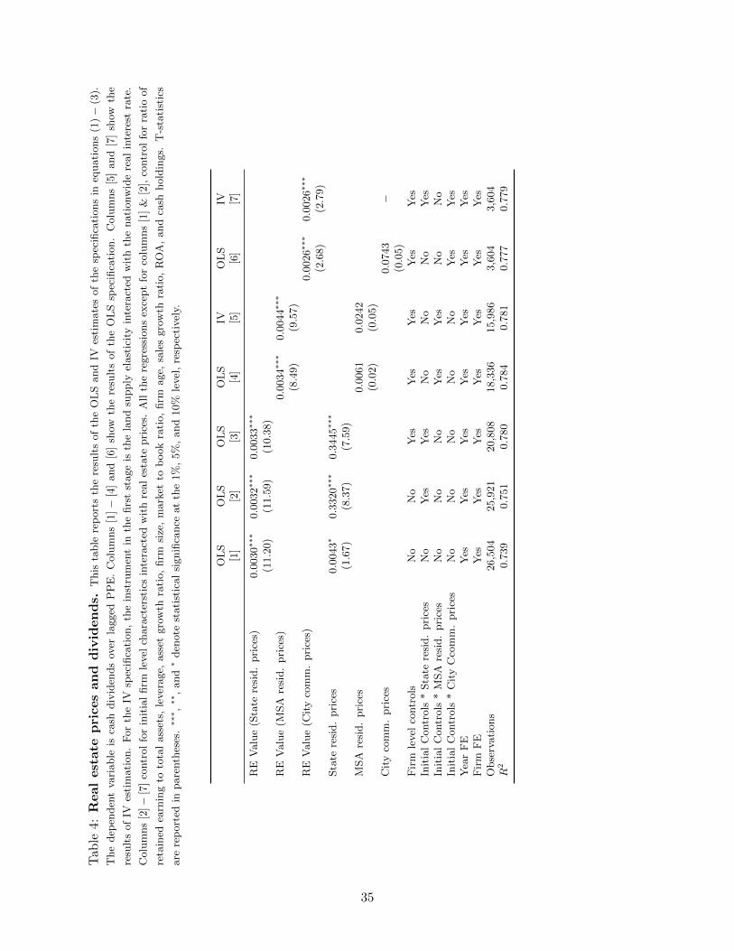
Tab

le4:

Real

est

ate

pri

ces

and

div

iden

ds.

This

table

rep

ort

sth

ere

sult

sof

the

OL

Sand

IVes

tim

ate

sof

the

spec

ifica

tions

ineq

uati

ons

(1)−

(3).

The

dep

enden

tva

riable

isca

shdiv

iden

ds

over

lagged

PP

E.

Colu

mns

[1]−

[4]

and

[6]

show

the

resu

lts

of

the

OL

Ssp

ecifi

cati

on.

Colu

mns

[5]

and

[7]

show

the

resu

lts

of

IVes

tim

ati

on.

For

the

IVsp

ecifi

cati

on,

the

inst

rum

ent

inth

efirs

tst

age

isth

ela

nd

supply

elast

icit

yin

tera

cted

wit

hth

enati

onw

ide

real

inte

rest

rate

.

Colu

mns

[2]−

[7]

contr

ol

for

init

ial

firm

level

chara

cter

stic

sin

tera

cted

wit

hre

al

esta

tepri

ces.

All

the

regre

ssio

ns

exce

pt

for

colu

mns

[1]

&[2

],co

ntr

ol

for

rati

oof

reta

ined

earn

ing

toto

tal

ass

ets,

lever

age,

ass

etgro

wth

rati

o,

firm

size

,m

ark

etto

book

rati

o,

firm

age,

sale

sgro

wth

rati

o,

RO

A,

and

cash

hold

ings.

T-s

tati

stic

s

are

rep

ort

edin

pare

nth

eses

.∗∗∗,∗∗

,and∗

den

ote

stati

stic

al

signifi

cance

at

the

1%

,5%

,and

10%

level

,re

spec

tivel

y.

OL

SO

LS

OL

SO

LS

IVO

LS

IV[1

][2

][3

][4

][5

][6

][7

]

RE

Valu

e(S

tate

resi

d.

pri

ces)

0.0

030∗∗∗

0.0

032∗∗∗

0.0

033∗∗∗

(11.2

0)

(11.5

9)

(10.3

8)

RE

Valu

e(M

SA

resi

d.

pri

ces)

0.0

034∗∗∗

0.0

044∗∗∗

(8.4

9)

(9.5

7)

RE

Valu

e(C

ity

com

m.

pri

ces)

0.0

026∗∗∗

0.0

026∗∗∗

(2.6

8)

(2.7

9)

Sta

tere

sid.

pri

ces

0.0

043∗

0.3

320∗∗∗

0.3

445∗∗∗

(1.6

7)

(8.3

7)

(7.5

9)

MSA

resi

d.

pri

ces

0.0

061

0.0

242

(0.0

2)

(0.0

5)

Cit

yco

mm

.pri

ces

0.0

743

−(0

.05)

Fir

mle

vel

contr

ols

No

No

Yes

Yes

Yes

Yes

Yes

Init

ial

Contr

ols

*Sta

tere

sid.

pri

ces

No

Yes

Yes

No

No

No

Yes

Init

ial

Contr

ols

*M

SA

resi

d.

pri

ces

No

No

No

Yes

Yes

No

No

Init

ial

Contr

ols

*C

ity

Cco

mm

.pri

ces

No

No

No

No

No

Yes

Yes

Yea

rF

EY

esY

esY

esY

esY

esY

esY

esF

irm

FE

Yes

Yes

Yes

Yes

Yes

Yes

Yes

Obse

rvati

ons

26,5

04

25,9

21

20,8

08

18,3

36

15,9

86

3,6

04

3,6

04

R2

0.7

39

0.7

51

0.7

80

0.7

84

0.7

81

0.7

77

0.7

79

35

Tab

le5:

Real

est

ate

pri

ces

an

dsh

are

rep

urc

hase

s.T

his

table

rep

ort

sth

ere

sult

sof

the

OL

Sand

IVes

tim

ate

sof

the

spec

ifica

tions

ineq

uati

ons

(1)-

(3).

The

dep

enden

tva

riable

issh

are

repurc

hase

sov

erla

gged

PP

E.

Colu

mn

[1]−

[4]

and

[6]

show

the

resu

lts

of

the

OL

Ssp

ecifi

cati

on,

while

colu

mns

[5]

and

[7]

show

the

resu

lts

of

IVes

tim

ati

on.

For

the

IVsp

ecifi

cati

on,

the

inst

rum

ent

inth

efirs

tst

age

isth

ela

nd

supply

elast

icit

yin

tera

cted

wit

hth

enati

onw

ide

inte

rest

rate

.C

olu

mns

[2]−

[7]

contr

ol

for

init

ial

firm

level

chara

cter

stic

sin

tera

cted

wit

hre

al

esta

tepri

ces.

All

the

regre

ssio

ns

exce

pt

for

colu

mns

[1]

&[2

],co

ntr

ol

for

rati

o

of

reta

ined

earn

ing

toto

tal

ass

ets,

lever

age,

ass

etgro

wth

rati

o,

firm

size

,m

ark

etto

book

rati

o,

firm

age,

sale

sgro

wth

rati

o,

RO

A,

and

cash

hold

ings.

T-s

tati

stic

s

are

rep

ort

edin

pare

nth

eses

.∗∗∗,∗∗

,and∗

den

ote

stati

stic

al

signifi

cance

at

the

1%

,5%

,and

10%

level

,re

spec

tivel

y.

OL

SO

LS

OL

SO

LS

IVO

LS

IV[1

][2

][3

][4

][5

][6

][7

]

RE

Valu

e(S

tate

resi

d.

pri

ces)

0.0

009∗∗

0.0

008∗

0.0

029∗∗∗

(1.9

9)

(1.7

3)

(5.2

3)

RE

Valu

e(M

SA

resi

d.

pri

ces)

0.0

033∗∗∗

0.0

041∗∗∗

(4.5

0)

(5.0

2)

RE

Valu

e(C

ity

com

m.

pri

ces)

0.0

056∗∗∗

0.0

057∗∗∗

(3.4

5)

(3.5

4)

Sta

tere

sid.

pri

ces

−0.0

080∗

0.0

354

0.1

187

(-1.8

8)

(0.5

3)

(1.4

1)

MSA

resi

d.

pri

ces

−0.2

652

−0.3

612

(-0.4

1)

(-0.4

0)

Cit

yco

mm

.pri

ces

−0.4

582

−(-

0.1

7)

Fir

mle

vel

contr

ols

No

No

Yes

Yes

Yes

Yes

Yes

Init

ial

Contr

ols

*Sta

tere

sid.

pri

ces

No

Yes

Yes

No

No

No

Yes

Init

ial

Contr

ols

*M

SA

resi

d.

pri

ces

No

No

No

Yes

Yes

No

No

Init

ial

Contr

ols

*C

ity

Cco

mm

.pri

ces

No

No

No

No

No

Yes

Yes

Yea

rF

EY

esY

esY

esY

esY

esY

esY

esF

irm

FE

Yes

Yes

Yes

Yes

Yes

Yes

Yes

Obse

rvati

ons

25,0

02

24,4

96

19,6

27

17,2

42

15,0

42

3,3

73

3,3

73

R2

0.3

97

0.4

11

0.4

44

0.4

49

0.4

55

0.4

87

0.4

87

36

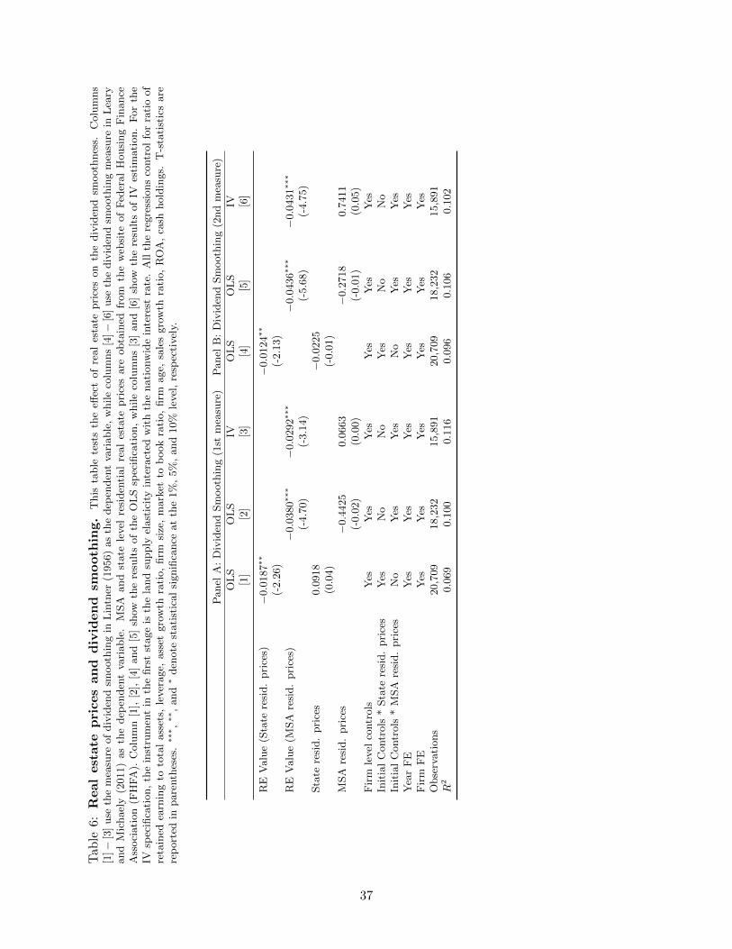
Tab

le6:

Real

est

ate

pri

ces

an

dd

ivid

en

dsm

ooth

ing.

This

table

test

sth

eeff

ect

of

real

esta

tepri

ces

on

the

div

iden

dsm

ooth

nes

s.C

olu

mns

[1]−

[3]

use

the

mea

sure

of

div

iden

dsm

ooth

ing

inL

intn

er(1

956)

as

the

dep

enden

tva

riable

,w

hile

colu

mns

[4]−

[6]

use

the

div

iden

dsm

ooth

ing

mea

sure

inL

eary

and

Mic

hael

y(2

011)

as

the

dep

enden

tva

riable

.M

SA

and

state

level

resi

den

tial

real

esta

tepri

ces

are

obta

ined

from

the

web

site

of

Fed

eral

Housi

ng

Fin

ance

Ass

oci

ati

on

(FH

FA

).C

olu

mn

[1],

[2],

[4]

and

[5]

show

the

resu

lts

of

the

OL

Ssp

ecifi

cati

on,

while

colu

mns

[3]

and

[6]

show

the

resu

lts

of

IVes

tim

ati

on.

For

the

IVsp

ecifi

cati

on,

the

inst

rum

ent

inth

efirs

tst

age

isth

ela

nd

supply

elast

icit

yin

tera

cted

wit

hth

enati

onw

ide

inte

rest

rate

.A

llth

ere

gre

ssio

ns

contr

ol

for

rati

oof

reta

ined

earn

ing

toto

tal

ass

ets,

lever

age,

ass

etgro

wth

rati

o,

firm

size

,m

ark

etto

book

rati

o,

firm

age,

sale

sgro

wth

rati

o,

RO

A,

cash

hold

ings.

T-s

tati

stic

sare

rep

ort

edin

pare

nth

eses

.∗∗∗,∗∗

,and∗

den

ote

stati

stic

al

signifi

cance

at

the

1%

,5%

,and

10%

level

,re

spec

tivel

y.

Panel

A:

Div

iden

dSm

ooth

ing

(1st

mea

sure

)P

anel

B:

Div

iden

dSm

ooth

ing

(2nd

mea

sure

)

OL

SO

LS

IVO

LS

OL

SIV

[1]

[2]

[3]

[4]

[5]

[6]

RE

Valu

e(S

tate

resi

d.

pri

ces)

−0.0

187∗∗

−0.0

124∗∗

(-2.2

6)

(-2.1

3)

RE

Valu

e(M

SA

resi

d.

pri

ces)

−0.0

380∗∗∗

−0.0

292∗∗∗

−0.0

436∗∗∗

−0.0

431∗∗∗

(-4.7

0)

(-3.1

4)

(-5.6

8)

(-4.7

5)

Sta

tere

sid.

pri

ces

0.0

918

−0.0

225

(0.0

4)

(-0.0

1)

MSA

resi

d.

pri

ces

−0.4

425

0.0

663

−0.2

718

0.7

411

(-0.0

2)

(0.0

0)

(-0.0

1)

(0.0

5)

Fir

mle

vel

contr

ols

Yes

Yes

Yes

Yes

Yes

Yes

Init

ial

Contr

ols

*Sta

tere

sid.

pri

ces

Yes

No

No

Yes

No

No

Init

ial

Contr

ols

*M

SA

resi

d.

pri

ces

No

Yes

Yes

No

Yes

Yes

Yea

rF

EY

esY

esY

esY

esY

esY

esF

irm

FE

Yes

Yes

Yes

Yes

Yes

Yes

Obse

rvati

ons

20,7

09

18,2

32

15,8

91

20,7

09

18,2

32

15,8

91

R2

0.0

69

0.1

00

0.1

16

0.0

96

0.1

06

0.1

02

37

Tab

le7:

Real

Est

ate

Pri

ces,

Div

iden

ds,

an

dS

hare

Rep

urc

hase

s:In

cre

asi

ng

(2002-2

007)

vs

decre

asi

ng

(2008-2

011)

real

est

ate

pri

ces.

This

table

test

sth

eeff

ect

of

real

esta

tepri

ces

on

the

div

iden

ds

and

share

repurc

hase

sduri

ng

boom

and

bust

per

iod.

The

dep

enden

tva

riable

inpanel

Aof

this

table

isca

shdiv

iden

dov

erla

gged

PP

Eand

inpanel

Bis

share

repurc

hase

over

lagged

PP

E.

The

regre

ssio

ns

use

din

panel

Aand

panel

Bare

sam

eas

the

ones

pre

sente

din

colu

mns

[1]−

[5]

of

table

4(f

or

panel

A)

and

of

table

5(f

or

panel

B).

All

the

regre

ssio

ns

exce

pt

for

colu

mns

[1],

[2],

[6],

&[7

]co

ntr

ol

for

rati

oof

reta

ined

earn

ing

toto

tal

ass

ets,

lever

age,

ass

etgro

wth

rati

o,

firm

size

,m

ark

etto

book

rati

o,

firm

age,

sale

sgro

wth

rati

o,

RO

A,

and

cash

hold

ings.

T-s

tati

stic

sare

rep

ort

edin

pare

nth

eses

.∗∗∗,∗∗

,and∗

den

ote

stati

stic

al

signifi

cance

at

the

1%

,5%

,and

10%

level

,re

spec

tivel

y.

Boom

Per

iod

(2002-2

007)

Bust

Per

iod

(2008-2

011)

OL

SO

LS

OL

SO

LS

IVO

LS

OL

SO

LS

OL

SIV

[1]

[2]

[3]

[4]

[5]

[6]

[7]

[8]

[9]

[10]

Panel

A:

Dep

enden

tV

ari

able

-D

ivid

end

Paid

RE

Valu

e(S

tate

resi

d.

pri

ces)

0.0

036∗∗∗

0.0

033∗∗∗

0.0

037∗∗∗

−0.0

013

−0.0

009

−0.0

015

(4.9

3)

(4.4

2)

(4.7

2)

(-0.7

3)

(-0.5

)(-

0.7

7)

RE

Valu

e(M

SA

resi

d.

pri

ces)

0.0

038∗∗∗

0.0

069∗∗∗

−0.0

002

−0.0

016

(3.8

2)

(6.1

4)

(-0.0

9)

(-0.5

9)

Sta

tere

sid.

Pri

ces

0.0

045

0.2

885∗∗∗

0.2

553∗∗

0.0

173

0.2

367

0.1

793

(1.0

4)

(2.7

3)

(2.4

5)

(1.5

1)

(0.5

0)

(0.3

8)

MSA

resi

d.

Pri

ces

−0.0

454

−0.0

802

0.3

879

−0.0

113

(-0.0

6)

(-0.2

4)

(0.6

0)

(-0.0

5)

Obse

rvati

ons

5,9

05

5,8

41

5,2

43

4,5

84

4,0

31

2,7

13

2,6

97

2,5

05

2,1

96

1,9

22

R2

0.8

63

0.8

77

0.8

91

0.8

96

0.8

97

0.8

83

0.8

90

0.8

98

0.8

98

0.8

93

Panel

B:

Dep

enden

tV

ari

able

-Share

sR

epurc

hase

d

RE

Valu

e(S

tate

resi

d.

pri

ces)

0.0

041∗∗∗

0.0

026∗

0.0

049∗∗∗

0.0

033

0.0

031

0.0

051

(3.1

0)

(1.8

6)

(3.1

6)

(1.1

0)

(0.9

7)

(1.5

1)

RE

Valu

e(M

SA

resi

d.

pri

ces)

0.0

060∗∗∗

0.0

090∗∗∗

0.0

069

0.0

056

(2.9

4)

(3.8

6)

(1.5

8)

(1.1

8)

Sta

tere

sid.

Pri

ces

−0.0

141∗

0.2

858

0.2

162∗∗

−0.0

334∗

−0.3

466

−0.5

993

(-1.7

5)

(1.0

3)

(0.7

5)

(-1.7

3)

(-0.4

4)

(-0.7

3)

MSA

resi

d.

Pri

ces

−2.0

413

−1.1

455∗

1.4

966

−0.7

364∗

(-1.4

1)

(-1.6

7)

(1.3

1)

(-1.7

2)

Obse

rvati

ons

5,5

01

5,4

51

4,8

99

4,2

63

3,7

57

2,6

02

2,5

89

2,4

03

2,1

00

1,8

42

R2

0.6

07

0.6

29

0.6

39

0.6

49

0.6

58

0.6

67

0.6

87

0.6

86

0.6

91

0.6

85

Fir

mle

vel

contr

ols

No

No

Yes

Yes

Yes

No

No

Yes

Yes

Yes

Inti

al

Contr

ols

*Sta

tere

sid.

Pri

ces

No

Yes

Yes

No

No

No

Yes

Yes

No

No

Inti

al

Contr

ols

*M

SA

resi

d.

Pri

ces

No

No

No

Yes

Yes

No

No

No

Yes

Yes

Yea

rF

EY

esY

esY

esY

esY

esY

esY

esY

esY

esY

esF

irm

FE

Yes

Yes

Yes

Yes

Yes

Yes

Yes

Yes

Yes

Yes

38

Tab

le8:

Real

Est

ate

Pri

ces,

Div

iden

ds,

an

dS

hare

Rep

urc

hase

:L

evera

ge

eff

ect

duri

ng

bu

stp

eri

od

(2008-2

011).

This

table

test

sth

eeff

ect

of

real

esta

tepri

ces

on

the

div

iden

ds

and

share

repurc

hase

sfo

rver

yhig

hand

ver

ylo

wle

ver

aged

firm

sduri

ng

the

bust

per

iod.

The

dep

enden

t

vari

able

inpanel

Aof

this

table

isca

shdiv

iden

dov

erla

gged

PP

Eand

inpanel

Bis

share

repurc

hase

over

lagged

PP

E.

The

regre

ssio

ns

use

din

panel

Aand

panel

Bare

sam

eas

the

ones

pre

sente

din

colu

mns

[1]−

[5]

of

table

4(f

or

panel

A)

and

of

table

5(f

or

panel

B).

All

the

regre

ssio

ns

exce

pt

for

colu

mns

[1],

[2],

[6],

&[7

]

inb

oth

the

panel

s,co

ntr

ol

for

rati

oof

reta

ined

earn

ing

toto

tal

ass

ets,

lever

age,

ass

etgro

wth

rati

o,

firm

size

,m

ark

etto

book

rati

o,

firm

age,

sale

sgro

wth

rati

o,

RO

A,

and

cash

hold

ings.

T-s

tati

stic

sare

rep

ort

edin

pare

nth

eses

.∗∗∗,∗∗

,and∗

den

ote

stati

stic

al

signifi

cance

at

the

1%

,5%

,and

10%

level

,re

spec

tivel

y.

Hig

hle

ver

aged

firm

sL

owle

ver

aged

firm

sO

LS

OL

SO

LS

OL

SIV

OL

SO

LS

OL

SO

LS

IV[1

][2

][3

][4

][5

][6

][7

][8

][9

][1

0]

Panel

A:

Dep

enden

tV

ari

able

-D

ivid

end

Paid

RE

Valu

e(S

tate

resi

d.

pri

ces)

0.0

036

0.0

057

0.0

058∗

−0.0

166∗∗∗

−0.0

129∗∗

−0.0

136∗∗

(1.2

0)

(1.6

3)

(1.9

4)

(-3.9

2)

(-2.5

5)

(-2.4

7)

RE

Valu

e(M

SA

resi

d.

pri

ces)

0.0

065∗

0.0

054

−0.0

193∗∗∗

−0.0

270∗∗∗

(1.7

6)

(1.1

9)

(-2.5

9)

(-3.1

4)

Sta

tere

sid.

Pri

ces

0.0

112

−1.0

777

−1.0

163

0.0

689∗∗

0.1

401

−0.0

561

(0.6

1)

(-1.4

2)

(-1.2

3)

(2.3

6)

(0.0

0)

(-0.0

0)

MSA

resi

d.

Pri

ces

0.4

253

−0.1

801

−6.8

753

3.6

221

(0.4

1)

(-0.5

4)

(-1.4

1)

(0.1

8)

Obse

rvati

ons

815

809

713

611

532

808

807

761

661

583

R2

0.9

21

0.9

33

0.9

62

0.9

61

0.9

55

0.8

48

0.8

82

0.8

87

0.8

81

0.8

82

Panel

B:

Dep

enden

tV

ari

able

-Share

sR

epurc

hase

d

RE

Valu

e(S

tate

resi

d.

pri

ces)

0.0

025

0.0

028

0.0

034

−0.0

020

−0.0

107

−0.0

072

(0.5

0)

(0.4

9)

(0.5

2)

(-0.3

2)

(-1.3

4)

(-0.8

2)

RE

Valu

e(M

SA

resi

d.

pri

ces)

0.0

069

0.0

083

−0.1

060

−0.0

097

(0.9

0)

(0.9

3)

(-0.8

5)

(-0.6

8)

Sta

tere

sid.

Pri

ces

−0.0

167

0.3

427

0.4

490

−0.0

200

−6.0

272

−4.4

154

(-0.5

4)

(0.2

8)

(0.2

5)

(-0.4

5)

(-1.1

4)

(-0.6

6)

MSA

resi

d.

Pri

ces

−0.5

357

−0.5

313

3.5

702

5.9

283

(-0.2

2)

(-0.8

0)

(0.4

4)

(0.1

9)

Obse

rvati

ons

782

778

683

587

508

769

768

710

624

550

R2

0.7

67

0.8

11

0.8

24

0.8

41

0.8

35

0.6

63

0.7

14

0.7

16

0.7

08

0.7

70

Fir

mle

vel

contr

ols

No

No

Yes

Yes

Yes

No

No

Yes

Yes

Yes

Inti

al

Contr

ols

*Sta

tere

sid.

Pri

ces

No

Yes

Yes

No

No

No

Yes

Yes

No

No

Inti

al

Contr

ols

*M

SA

resi

d.

Pri

ces

No

No

No

Yes

Yes

No

No

No

Yes

Yes

Yea

rF

EY

esY

esY

esY

esY

esY

esY

esY

esY

esY

esF

irm

FE

Yes

Yes

Yes

Yes

Yes

Yes

Yes

Yes

Yes

Yes

39

Tab

le9:

Real

Est

ate

Pri

ces,

Div

iden

ds,

an

dS

hare

Rep

urc

hase

:A

vailab

ilit

yof

Invest

ment

Op

port

un

itie

s.T

his

table

test

sth

e

effec

tof

real

esta

tepri

ces

on

the

div

iden

ds

and

share

repurc

hase

sco

ndit

ioned

on

the

availabilit

yof

inves

tmen

topp

ort

unit

ies.

Fir

ms

inb

ott

om

3dec

iles

of

Tobin

s

Qare

defi

ned

topro

xy

for

less

inves

tmen

topp

ort

unit

ies.

Sim

ilarl

y,firm

sin

top

3dec

iles

of

Tobin

sQ

are

defi

ned

topro

xy

for

hig

hin

ves

tmen

topp

ort

unit

ies.

The

dep

enden

tva

riable

inpanel

Aof

this

table

isca

shdiv

iden

dov

erla

gged

PP

Eand

inpanel

Bis

share

repurc

hase

over

lagged

PP

E.

The

regre

ssio

ns

use

din

panel

Aand

panel

Bare

sam

eas

the

ones

pre

sente

din

colu

mns

[1]−

[5]

of

table

4(f

or

panel

A)

and

of

table

5(f

or

panel

B).

All

the

regre

ssio

ns

exce

pt

for

colu

mns

[1],

[2],

[6],

&[7

]in

both

the

panel

s,co

ntr

ol

for

rati

oof

reta

ined

earn

ing

toto

tal

ass

ets,

lever

age,

ass

etgro

wth

rati

o,

firm

size

,m

ark

etto

book

rati

o,

firm

age,

sale

sgro

wth

rati

o,

RO

A,

and

cash

hold

ings.

T-s

tati

stic

sare

rep

ort

edin

pare

nth

eses

.∗∗∗,∗∗

,and∗

den

ote

stati

stic

al

signifi

cance

at

the

1%

,5%

,and

10%

level

,

resp

ecti

vel

y.

Fir

ms

wit

hle

ssin

ves

tmen

topp

ort

unit

ies

available

Fir

ms

wit

hm

ore

inves

tmen

topp

ort

unit

ies

available

OL

SO

LS

OL

SO

LS

IVO

LS

OL

SO

LS

OL

SIV

[1]

[2]

[3]

[4]

[5]

[6]

[7]

[8]

[9]

[10]

Panel

A:

Dep

enden

tV

ari

able

-D

ivid

end

Paid

RE

Valu

e(S

tate

resi

d.

pri

ces)

0.0

021∗∗∗

0.0

026∗∗∗

0.0

020∗∗∗

0.0

011∗∗∗

0.0

016∗∗∗

0.0

003

(4.9

5)

(5.8

8)

(4.0

5)

(2.1

7)

(3.0

0)

(0.5

2)

RE

Valu

e(M

SA

resi

d.

pri

ces)

0.0

016∗∗∗

0.0

021∗∗∗

0.0

007

0.0

011

(2.4

7)

(2.8

5)

(0.8

2)

(1.1

4)

Sta

tere

sid.

Pri

ces

0.0

110∗∗

0.0

260

0.0

131

−0.0

029

0.4

956∗∗∗

0.5

847∗∗∗

(2.5

0)

(0.2

1)

(0.0

5)

(-0.6

2)

(6.6

1)

(7.1

0)

MSA

resi

d.

Pri

ces

0.0

461

0.2

835

−0.0

007

−0.1

951

(0.0

7)

(0.4

1)

(-0.0

0)

(-0.4

5)

Obse

rvati

ons

7,5

88

7,4

86

6,3

54

5,4

94

4,6

97

8,8

13

8,5

26

6,0

43

5,4

94

4,8

35

R2

0.7

05

0.7

22

0.7

46

0.7

47

0.7

36

0.8

47

0.8

63

0.9

01

0.9

03

0.9

05

Panel

B:

Dep

enden

tV

ari

able

-Share

sR

epurc

hase

d

RE

Valu

e(S

tate

resi

d.

pri

ces)

0.0

026∗∗∗

0.0

029∗∗∗

0.0

043∗∗∗

−0.0

021∗∗

−0.0

020∗∗

−0.0

007

(3.7

7)

(4.0

6)

(5.0

7)

(-2.3

2)

(-2.1

5)

(-0.4

9)

RE

Valu

e(M

SA

resi

d.

pri

ces)

0.0

042∗∗∗

0.0

051∗∗∗

−0.0

005

−0.0

008

(3.7

1)

(3.9

4)

(-0.2

6)

(-0.4

0)

Sta

tere

sid.

Pri

ces

−0.0

085

−0.0

839

−0.1

798

−0.0

082

0.1

597

−0.2

275

(-1.2

1)

(-0.4

2)

(-0.4

2)

(-0.9

8)

(0.8

4)

(-0.5

9)

MSA

resi

d.

Pri

ces

−0.1

653

0.0

060

−0.1

953

−0.1

780

(-0.1

4)

(0.0

1)

(-0.4

4)

(-0.1

3)

Obse

rvati

ons

7,2

83

7,1

92

6,1

20

5,2

73

4,4

94

8,1

61

7,9

21

5,5

44

5,0

27

4,4

50

R2

0.4

19

0.4

38

0.4

80

0.4

88

0.4

90.5

67

0.5

91

0.6

19

0.6

26

0.6

35

Fir

mle

vel

contr

ols

No

No

Yes

Yes

Yes

No

No

Yes

Yes

Yes

Inti

al

Contr

ols

*Sta

tere

sid.

Pri

ces

No

Yes

Yes

No

No

No

Yes

Yes

No

No

Inti

al

Contr

ols

*M

SA

resi

d.

Pri

ces

No

No

No

Yes

Yes

No

No

No

Yes

Yes

Yea

rF

EY

esY

esY

esY

esY

esY

esY

esY

esY

esY

esF

irm

FE

Yes

Yes

Yes

Yes

Yes

Yes

Yes

Yes

Yes

Yes

40

Table 10: Real estate prices and payout: Robustness tests 1 and 2. This table tests the

robustness of the effect of real estate prices on the payout policy of the firm. The baseline regression is the specification

in column [4] of Table 4. Dependent variables in columns [1] and [3] are the ratio of cash dividend to lagged property,

plant and equipment (PPE) and share repurchase to lagged PPE, respectively in lower 3 quartile of firm size and

in the largest 20 MSAs. Dependent variables in columns [2] and [4] are the average dividend over the next 3 years

normalized by lagged PPE, and average share repurchase over next 3 years normalized by lagged PPE. MSA level

esidential real estate prices are obtained from the website of Federal Housing Finance Association (FHFA). All

regressions use MSA-level residential prices, year and firm fixed effect, control for ratio of retained earning to total

assets, leverage, asset growth ratio, firm size, market to book ratio, firm age, sales growth ratio, ROA, cash holdings,

and initial controls interacted with MSA-level residential prices. Standard errors are clustered at the MSA-year level.

T-statistics are reported in parentheses. ∗∗∗, ∗∗, and ∗ denote statistical significance at the 1%, 5%, and 10% level,

respectively.

Dividend/lagged PPE Share Repurchases/lagged PPE

Large MSAs 3-year mean Large MSAs 3-year mean& small firms dividend & small firms repurchase

[1] [2] [3] [4]

RE Value (MSA resid. prices) 0.0054∗∗∗ 0.0068∗∗∗ 0.0035∗∗∗ 0.0117∗∗∗

(8.09) (12.09) (2.95) (6.24)MSA resid. prices −0.2469 0.0653 −0.4036 0.0979

(-0.40) (0.07) (-0.38) (0.03)Firm level controls Yes Yes Yes YesInitial Controls * MSA resid. prices Yes Yes Yes YesYear FE Yes Yes Yes YesFirm FE Yes Yes Yes YesObservations 7,890 14,933 7,401 13,260R2 0.778 0.784 0.457 0.579

41

Tab

le11

:R

eal

est

ate

pri

ces

an

dp

ayou

t:R

ob

ust

ness

test

3.

Inth

ista

ble

,w

ete

stth

ero

butn

ess

of

the

effec

tof

real

esta

tepri

ces

on

the

pay

out

policy

of

the

firm

for

old

erfirm

sto

mit

igate

the

endogen

eity

pro

ble

mass

oci

ate

dw

ith

choic

eof

bei

ng

loca

ted

ina

part

icula

rst

ate

or

MSA

.T

he

dep

enden

t

vari

able

inco

lum

ns

[1]−

[3]

isca

shdiv

iden

dov

erla

gged

PP

Eand

inco

lum

ns

[4]−

[6]

issh

are

repurc

hase

dov

erla

gged

PP

E.

The

regre

ssio

ns

use

din

colu

mns

[1]−

[3]

are

sam

eas

the

ones

pre

sente

din

colu

mns

[3],

[4],

and

[5]

of

table

4but

run

on

the

sam

ple

of

firm

sw

hic

hhav

eb

een

public

for

at

least

10

yea

rs.

Sim

ilarl

y,

regre

ssio

ns

use

din

colu

mns

[4]−

[6]

are

sam

eas

the

ones

pre

sente

din

colu

mns

[3],

[4],

and

[5]

of

table

5but

run

on

the

sam

ple

of

old

erfirm

s.A

llth

ere

gre

ssio

ns

contr

ol

for

rati

oof

reta

ined

earn

ing

toto

tal

ass

ets,

lever

age,

ass

etgro

wth

rati

o,

firm

size

,m

ark

etto

book

rati

o,

firm

age,

sale

sgro

wth

rati

o,

RO

A,

cash

hold

ings.

T-s

tati

stic

sare

rep

ort

edin

pare

nth

eses

.∗∗∗,∗∗

,and∗

den

ote

stati

stic

al

signifi

cance

at

the

1%

,5%

,and

10%

level

,re

spec

tivel

y.

Panel

AP

anel

BD

ivid

end/la

gged

PP

EShare

Rep

urc

hase

/la

gged

PP

E

OL

SO

LS

IVO

LS

OL

SIV

[1]

[2]

[3]

[4]

[5]

[6]

RE

Valu

e(S

tate

resi

d.

pri

ces)

0.0

031∗∗∗

0.0

029∗∗∗

(8.6

5)

(4.8

8)

RE

Valu

e(M

SA

resi

d.

pri

ces)

0.0

036∗∗∗

0.0

046∗∗∗

0.0

031∗∗∗

0.0

038∗∗∗

(7.8

6)

(8.8

4)

(4.0

1)

(4.3

3)

Sta

tere

sid.

Pri

ces

0.1

743∗∗

0.0

212

(2.1

2)

(0.1

5)

MSA

resi

d.

Pri

ces

0.2

026

0.0

646

−0.4

336

−0.4

534∗

(0.8

9)

(0.4

6)

(-1.1

5)

(-1.9

4)

Fir

mle

vel

contr

ols

Yes

Yes

Yes

Yes

Yes

Yes

Init

ial

Contr

ols

*Sta

tere

sid.

Pri

ces

Yes

No

No

Yes

No

No

Init

ial

Contr

ols

*M

SA

resi

d.

Pri

ces

No

Yes

Yes

No

Yes

Yes

Yea

rF

EY

esY

esY

esY

esY

esY

esF

irm

FE

Yes

Yes

Yes

Yes

Yes

Yes

Obse

rvati

ons

16,4

19

14,4

67

12,5

90

15,6

03

13,7

03

11,9

26

R2

0.7

92

0.7

94

0.7

92

0.4

75

0.4

78

0.4

83

42

Tab

le12

:R

eal

est

ate

pri

ces

an

dd

ivid

en

dp

ayou

t:R

ob

ust

ness

test

4.

This

table

test

sth

eeff

ect

of

real

esta

tepri

ces

on

the

div

iden

d

pay

out

acc

ounti

ng

for

loca

tion

of

firm

s.T

he

dep

enden

tva

riable

isca

shdiv

iden

dov

erla

gged

PP

E.

The

regre

ssio

ns

use

dare

sam

eas

the

ones

pre

sente

din

colu

mns

[1]−

[5]

of

table

4w

ith

addit

ion

of

loca

tion

dum

my

and

inte

rati

on

of

real

esta

teva

lue

wit

hlo

cati

on

dum

my.

All

the

regre

ssio

ns

exce

pt

inco

lum

n[1

]and

[2]

contr

ol

for

rati

oof

reta

ined

earn

ing

toto

tal

ass

ets,

lever

age,

ass

etgro

wth

rati

o,

firm

size

,m

ark

etto

book

rati

o,

firm

age,

sale

sgro

wth

rati

o,

RO

A,

cash

hold

ings.

T-s

tati

stic

sare

rep

ort

edin

pare

nth

eses

.∗∗∗,∗∗

,and∗

den

ote

stati

stic

al

signifi

cance

at

the

1%

,5%

,and

10%

level

,re

spec

tivel

y.

OL

SO

LS

OL

SO

LS

IV[1

][2

][3

][4

][5

]

RE

Valu

e(S

tate

Res

iden

tial

Pri

ces)

0.0

026∗∗∗

0.0

019∗∗∗

0.0

016∗∗∗

(7.8

2)

(5.7

1)

(4.2

3)

RE

Valu

e(M

SA

Rei

den

tial

Pri

ces)

0.0

025∗∗∗

0.0

035∗∗∗

(5.3

2)

(6.2

6)

Cen

tral

Loca

tion

−0.0

010

−0.0

041∗

−0.0

061∗∗∗

−0.0

047∗∗

−0.0

049∗

(-0.6

8)

(1.9

3)

(-2.9

1)

(-2.1

7)

(-1.8

2)

Cen

tral

Loca

tion*R

EV

alu

e0.0

011∗∗

0.0

009∗

0.0

013∗∗

0.0

018∗

0.0

001

(2.2

1)

(1.8

1)

(2.4

9)

(1.7

6)

(0.1

5)

Sta

teR

esid

enti

al

Pri

ces

0.0

081∗∗∗

0.1

379∗∗∗

0.1

236∗∗∗

(3.2

0)

(3.8

3)

(3.0

0)

MSA

Rei

den

tial

Pri

ces

−0.0

070

−0.0

064

(-0.0

8)

(-0.1

0)

Fir

mle

vel

contr

ols

No

No

Yes

Yes

Yes

Init

ial

Contr

ols

*Sta

teR

es.

Pri

ces

No

Yes

Yes

No

No

Init

ial

Contr

ols

*M

SA

Res

.P

rice

sN

oN

oN

oY

esY

esY

ear

FE

Yes

Yes

Yes

Yes

Yes

Fir

mF

EY

esY

esY

esY

esY

esO

bse

rvati

ons

24,1

55

23,6

32

19,2

17

18,3

36

15,9

86

R2

0.0

57

0.3

50

0.4

17

0.4

19

0.4

22

43

Tab

le13

:R

eal

est

ate

pri

ces

an

dp

ayou

t:R

ob

ust

ness

test

5a.

This

table

test

sth

ero

butn

ess

of

the

effec

tof

real

esta

tepri

ces

on

the

pay

out

policy

of

the

firm

while

contr

ollin

gfo

rth

ein

ves

tmen

t.T

he

dep

enden

tva

riable

inco

lum

ns

[1]−

[3]

isca

shdiv

iden

dov

erla

gged

PP

Eand

inco

lum

ns

[4]−

[6]

is

share

repurc

hase

dov

erla

gged

PP

E.T

he

regre

ssio

ns

use

din

colu

mns

[1]−

[3]are

sam

eas

the

ones

pre

sente

din

colu

mns

[3],

[4],

and

[5]of

table

4w

ith

an

addit

ional

contr

ol

of

inves

tmen

t.Sim

ilarl

y,re

gre

ssio

ns

use

din

colu

mns

[4]−

[6]

are

sam

eas

the

ones

pre

sente

din

colu

mns

[3],

[4],

and

[5]

of

table

5w

ith

an

addit

ional

conto

lof

inves

tmen

t.In

ves

tmen

tva

riable

isdefi

ned

as

capit

al

exp

endit

ure

norm

alize

dby

lagged

PP

E.

All

the

regre

ssio

ns

contr

ol

for

rati

oof

reta

ined

earn

ing

to

tota

lass

ets,

lever

age,

ass

etgro

wth

rati

o,

firm

size

,m

ark

etto

book

rati

o,

firm

age,

sale

sgro

wth

rati

o,

RO

A,

cash

hold

ings,

and

init

ial

firm

level

chara

cter

stic

s

inte

ract

edw

ith

real

esta

tepri

ces.

T-s

tati

stic

sare

rep

ort

edin

pare

nth

eses

.∗∗∗,∗∗

,and∗

den

ote

stati

stic

al

signifi

cance

at

the

1%

,5%

,and

10%

level

,re

spec

tivel

y.

Div

iden

d/la

gged

PP

EShare

Rep

urc

hase

/la

gged

PP

E

OL

SO

LS

IVO

LS

OL

SIV

[1]

[2]

[3]

[4]

[5]

[6]

RE

Valu

e(S

tate

resi

d.

pri

ces)

0.0

030∗∗∗

0.0

026∗∗∗

(9.3

5)

(4.6

5)

RE

Valu

e(M

SA

resi

d.

pri

ces)

0.0

034∗∗∗

0.0

044∗∗∗

0.0

030∗∗∗

0.0

039∗∗∗

(8.3

4)

(9.4

0)

(4.1

1)

(4.7

5)

Sta

tere

sid.

Pri

ces

0.3

445∗∗∗

0.1

187

(7.5

9)

(1.4

1)

MSA

resi

d.

Pri

ces

0.0

103

0.0

272

−0.2

607

−0.3

606

(0.0

3)

(0.0

5)

(-0.4

0)

(-0.4

0)

Inves

tmen

t0.0

011

0.0

008

0.0

006

0.0

040∗∗∗

0.0

036∗∗∗

0.0

032∗∗

(1.5

9)

(0.1

4)

(0.8

0)

(3.3

5)

(2.8

1)

(2.3

6)

Fir

mle

vel

contr

ols

Yes

Yes

Yes

Yes

Yes

Yes

Init

ial

Contr

ols

*Sta

tere

sid.

Pri

ces

Yes

No

No

Yes

No

No

Init

ial

Contr

ols

*M

SA

resi

d.

Pri

ces

No

Yes

Yes

No

Yes

Yes

Yea

rF

EY

esY

esY

esY

esY

esY

esF

irm

FE

Yes

Yes

Yes

Yes

Yes

Yes

Obse

rvati

ons

20,6

31

18,1

94

15,8

57

19,4

60

17,1

06

14,9

19

R2

0.7

81

0.7

83

0.7

79

0.4

45

0.4

50

0.4

56

44

Tab

le14

:R

eal

est

ate

pri

ces

an

dd

ivid

en

dsm

ooth

ing:

Rob

ust

ness

test

5b

.T

his

table

test

sth

eeff

ect

of

real

esta

tepri

ces

on

the

div

iden

dsm

ooth

nes

sw

hile

contr

ollin

gfo

rth

ein

ves

tmen

t.T

he

base

line

regre

ssio

nis

the

spec

ifica

tion

inco

lum

n[1

],[2

],and

[3]

of

table

6.

Colu

mns

[1]−

[3]

use

tradit

ional

use

dm

easu

reof

div

iden

dsm

ooth

ing

as

dep

enden

tva

riable

,w

hile

colu

mns

[4]−

[6]

use

div

iden

dsm

ooth

ing

mea

sure

as

use

din

Lea

ryand

Mic

hael

y(2

011)

as

the

dep

enden

tva

riable

.The

regre

ssio

ns

use

dare

sam

eas

the

ones

pre

sente

dta

ble

6w

ith

an

addit

ional

contr

ol

of

inves

tmen

t.In

ves

tmen

tva

riable

isdefi

ned

as

capit

al

exp

endit

ure

norm

alize

dby

lagged

PP

E.

All

the

regre

ssio

ns

contr

ol

for

rati

oof

reta

ined

earn

ing

toto

tal

ass

ets,

lever

age,

ass

etgro

wth

rati

o,

firm

size

,m

ark

etto

book

rati

o,

firm

age,

sale

sgro

wth

rati

o,

RO

A,

cash

hold

ings,

and

init

ial

firm

level

chara

cter

stic

sin

tera

cted

wit

hre

al

esta

tepri

ces.

T-s

tati

stic

sare

rep

ort

edin

pare

nth

eses

.∗∗∗,∗∗

,and∗

den

ote

stati

stic

al

signifi

cance

at

the

1%

,5%

,and

10%

level

,re

spec

tivel

y.

Div

iden

dSm

ooth

ing

(1st

mea

sure

)D

ivid

end

Sm

ooth

ing

(2nd

mea

sure

)

OL

SO

LS

IVO

LS

OL

SIV

[1]

[2]

[3]

[4]

[5]

[6]

RE

Valu

e(S

tate

resi

d.

pri

ces)

−0.0

181∗∗

−0.0

125∗∗

(-2.1

7)

(-2.1

1)

RE

Valu

e(M

SA

resi

d.

pri

ces)

−0.0

374∗∗∗

−0.0

283∗∗∗

−0.0

440∗∗∗

−0.0

437∗∗∗

(-4.6

0)

(-3.0

2)

(-5.6

8)

(-4.7

8)

Sta

tere

sid.

pri

ces

0.0

670

−0.0

513

(0.0

3)

(-0.0

3)

MSA

resi

d.

pri

ces

−0.3

876

−0.1

153

−0.2

012

0.5

103

(-0.0

2)

(-0.0

1)

(-0.0

1)

(0.0

3)

Inves

tmen

t0.0

431

0.0

245

0.0

309

0.0

332

0.0

367

0.0

429

(1.2

8)

(0.8

9)

(1.0

2)

(1.4

0)

(1.3

9)

(1.4

5)

Fir

mle

vel

contr

ols

Yes

Yes

Yes

Yes

Yes

Yes

Init

ial

Contr

ols

*Sta

tere

sid.

pri

ces

Yes

No

No

Yes

No

No

Init

ial

Contr

ols

*M

SA

resi

d.

pri

ces

No

Yes

Yes

No

Yes

Yes

Yea

rF

EY

esY

esY

esY

esY

esY

esF

irm

FE

Yes

Yes

Yes

Yes

Yes

Yes

Obse

rvati

ons

20,5

32

18,0

90

15,7

62

20,5

32

18,0

90

15,7

62

R2

0.0

69

0.1

01

0.1

16

0.0

97

0.1

07

0.1

03

45