1

Unemployment Rates Forecasts – Unobserved Component

Models versus SARIMA models

Barbara Będowska-Sójka1

Abstract:

In this paper we focus on the comparison of unemployment rates forecasting accuracy

using time-varying parameter models and SARIMA models. We are particularly interested in

the forecasts of the unemployment rate of eight Central and Eastern European first-wave

accession countries: Estonia, Latvia, Lithuania, Czech Republic, Poland, Slovakia, Hungary

and Slovenia within 1999-2015 years. We use a rolling short-term forecast experiment in

order to obtain out-of-sample test of forecast accuracy. Moreover, we examine also the

dynamic asymmetries in unemployment rates and the forecasting performance of different

models. We find that the forecasting ability of the models depends not only on the forecasting

horizon, but also on the direction of the movement in unemployment rates. The empirical

evidence derived from our investigation suggests that there is no best single model, however

SARIMA models although not including a “cyclical” component tend to perform better than

others for a longer forecasts horizons.

JEL classification codes: C22, C53, E27;

Keywords: unemployment rate, unobserved component, SARIMA models, forecasting

accuracy

1 Department of Econometrics, Poznan University of Economics, Al. Niepodległości 10, 61-875 Poznań, Poland,

Phone: +48 618543875, e-mail: barbara.bedowska-sojka@ue.poznan.pl;

2

Introduction

An important question in forecasting of time series is which model is the best one. For more

or less forty years ARMA-type models have been used for modelling and forecasting

economic time series. This approach has a certain feature: all shocks, coming either from the

cycle or from other sources, are included in these model’s innovations. Simultaneously in the

last years the unobserved component models seem to become very promising tool in

forecasting different economic series as it allows to separate time series components. In this

paper we compare the forecasting accuracy of few unobserved component models and few

specifications of seasonal autoregressive integrated moving average (SARIMA) models. We

are interested in comparison of different models of unemployment rates series in several

Central and Eastern European (CEE) countries..

Neftci [1984] indicate that some macroeconomic series display asymmetric behaviour.

In case of the unemployment rates they have a tendency to rise suddenly, but fall gradually

(Koop and Potter 1999). In this paper we are interested if there are the differences of the

unemployment rates’ forecasts accuracy at the time of increase and decrease of these rates.

For the purpose of forecasting we use linear models: in case of structural time series

modelling level, trend, seasonality and cyclical components are included, allowing for the

coefficients on each predictor to be either time variable or constant over time. In the case of

SARIMA models we consider two different specifications. The forecasting performance of

different models is compared in different horizons and different times in order to indicate the

best model.

A number of research papers have used time series models for forecasting

unemployment rates. These works are devoted either to single unemployment rate, where

clearly the most popular is the US unemployment rate (e.g. Montgomery et al. 1998,

Altissimo and Violante 2001, Caner and Hansen 2001, Proietti 2003, Koop and Potter 1999)

or a comparison of models used in forecasting unemployment rates from different economies,

eg. OECD countries (Skalin and Teräsvirta 2002, U.S., U.K., Canada, and Japan (Milas and

Rothman 2005), G7 countries (Teräsvirta et al. 2005) and the Baltic States (Będowska-Sójka

2015).

Many works are devoted to comparison of different models. Montgomery, Zarnowitz,

Tsay and Tiao [1998] in a rolling forecasts experiment for the US quarterly unemployment

3

rates show that non-linear models performed better than the linear ARMA model in terms of

forecasting errors when the unemployment increased rapidly but not elsewhere. Stock and

Watson [1999] used a large data set of U.S. macroeconomic time series, including the

monthly unemployment rate, and showed that linear models have better forecasting accuracy

than nonlinear ones. Oppositely, Teräsvirta et al. [2005] find that the nonlinear LSTAR model

turns out to be better than the linear or neural network models when modelling unemployment

rates in G7 countries.

Marcellino (2002) generated forecasts of three key economic variables: the growth

rate of industrial production, the unemployment rate and the inflation. He showed that best

forecast for industrial production was obtained within linear models, whereas for the

unemployment rate the non-linear models generate better forecasts. Proietti [2003]

investigated the out-of-sample performance of linear and nonlinear structural time series

models of the seasonally adjusted US unemployment rate. Generally linear models are said to

perform significantly better than nonlinear models, but a nonlinear specification outperforms

the selected linear model at short lead times in periods of slowly decreasing unemployment

rate.

The main purpose of this paper is to compare an accuracy of unemployment rate

forecast’s obtained from different linear models, namely structural time series models and

SARIMA models. Our approach is much in the same spirit of Proietti (2003) and Będowska-

Sójka (2015) as it concentrates on the comparison of forecasting models on the basis of the

short-term forecasts. With respect to Proietti (2003) paper we focus on seasonally unadjusted

data from several countries and use linear structural time series models only. In Będowska-

Sójka (2015) few unobserved component models are compared from the perspective of

forecasts generated for unemployment rates of the three Baltic states: Lithuania, Latvia and

Estonia. In that paper it is shown that models which contain cyclical components perform

better than other unobserved component models (Będowska-Sójka 2015).

Our sample data consists of seasonally unadjusted monthly unemployment rates of the

eight CEE countries that joined European Union in 2004 in the first-wave accession. These

countries are: Czech Republic, Estonia, Hungary, Latvia, Lithuania, Poland, Slovakia, and

Slovenia. The sample starts in January 1999 and ends in March 2015 (with some exceptions

described below). The forecasts of unemployment rates are generated from the rolling

forecasts experiment where seasonality effects are built directly into the forecasting

procedure. In this paper we consider all forecasts origin starting from January 2008 and

4

ending in March 2014. The forecasts are set to horizons from one month to one year. As the

rolling window generally consists of 108 observations we obtain 75 forecasts for each series

and each models. In order to compare forecasts from different models, we use common

forecasting error measures. To the best of our knowledge this is the first study that compares

unemployment rate forecasts within these eight CEE countries.

Our contribution is as follows: first in six out of eight cases seasonal ARIMA models

offered better forecasting accuracy than the unobserved component models. Second, when

comparing models across all countries in the sample, there are substantial differences between

their forecasting abilities; the lowest mean percentage forecasting error for 12-month horizon

is 1.82% in case of Slovakian unemployment rate and the highest is 8.67% for the Estonian

one. In case of Estonian, Latvian and Slovenian unemployment rates shocks that increase

unemployment rates tend to have greater negative impact on the model’s forecasting ability

than shocks that lower unemployment rate. Finally, the differences in forecasting errors

obtained from different methods are generally not serious.

The plan of the paper is as follows. Next section describes the methodology used in

the empirical study. Then data are presented and empirical results of the comparison of

forecasts are shown. In the last section the conclusions are presented.

Methodology

Our paper aims to compare forecasts from two alternative specifications that are used

to represent the dynamic properties of series, namely unobserved component models (UC)

and seasonal ARIMA models. When the disturbances are independent, identically distributed

and Gaussian, an ARIMA model with restrictions in the parameters is the reduced form of an

unobserved component model [Harvey 1989]. There is one aggregated disturbance within the

specification of ARIMA models, whereas unobserved component models include component

disturbances. Thus, the latter may allow to discover the characteristics, that are not observed

in the reduced form of ARIMA model. In this paper we try examine which of these two

classes of the models is more appropriate when forecasting the unemployment rates.

The theory of structural time series models and ARIMA models is presented by

Harvey [1989] – below a short presentation of the models used in the study is given.

Within ARIMA models we use two specifications:

I. Seasonal ARIMA(0,1,1)(0,1,1) – henceforth SARIMA1

5

II. Seasonal ARIMA(2,1,0)(0,1,1) – henceforth SARIMA2.

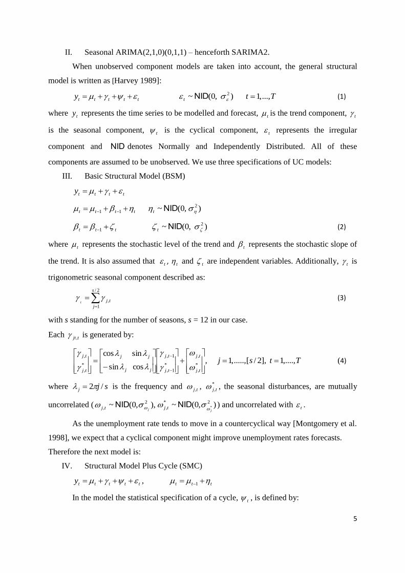
When unobserved component models are taken into account, the general structural

model is written as [Harvey 1989]:

ttttty Ttt ...,,1),0(~ 2 NID (1)

where ty represents the time series to be modelled and forecast, t is the trend component, t

is the seasonal component, t is the cyclical component, t represents the irregular

component and NID denotes Normally and Independently Distributed. All of these

components are assumed to be unobserved. We use three specifications of UC models:

III. Basic Structural Model (BSM)

tttty

),0(~ 2

11 NIDttttt

),0(~ 2

1 NIDtttt (2)

where t represents the stochastic level of the trend and t represents the stochastic slope of

the trend. It is also assumed that t , t and t are independent variables. Additionally, t is

trigonometric seasonal component described as:

2/

1

,

s

j

tjt (3)

with s standing for the number of seasons, s = 12 in our case.

Each tjt , is generated by:

Ttsjtj

tj

tj

tj

jj

jj

tj

tj

,....,1],2/[.....,,1,cossin

sincos

*

,

,

*

1,

1,

*

,

,

(4)

where sjj /2 is the frequency and tj , , *

,tj , the seasonal disturbances, are mutually

uncorrelated ( ),,0(~ 2

, jtj NID ),0(~ 2*

, *j

tj NID ) and uncorrelated with t .

As the unemployment rate tends to move in a countercyclical way [Montgomery et al.

1998], we expect that a cyclical component might improve unemployment rates forecasts.

Therefore the next model is:

IV. Structural Model Plus Cycle (SMC)

ttttty , ttt 1

In the model the statistical specification of a cycle, t , is defined by:

6

Ttt

t

t

t

cc

cc

t

t...,1,

cossin

sincos

**

1

1

*

(5)

where: c is the frequency (in radians), c0 , is a damping factor, 10 and

*, tt are mutually uncorrelated white noise disturbances with zero means and common

variance 2

.

The last model included in the study is:

V. Autoregressive Structural Model (ARSM)

ttttt yy 1 , ttt 1 ),0(~ 2

NIDt (6)

where t represents the stochastic level of the trend , t is trigonometric seasonal component

described in equations (3) and (4), t represents the irregular component (as in equation 1).

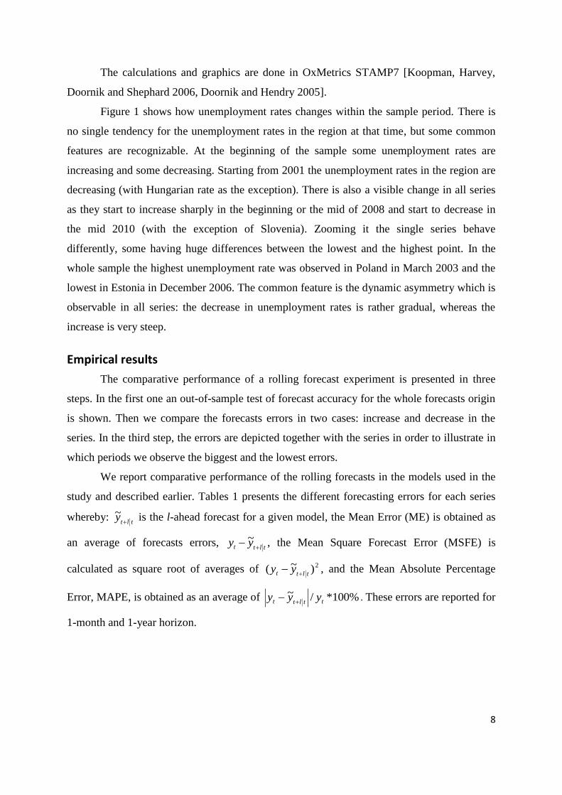
As the primary use of time series models is forecasting, it seems that mean square

error MSE would be adequate criterion in judging the models performance [Montgomery et

al. 1998]. We use out-of-sample forecasts to assess which model gives the better accuracy.

These forecasts are generated in a rolling forecasts window: for the given origin the model is

estimated and forecasts are generated. Next, this step is repeated for each model and each

series – hence we obtain 75 forecasts from one-step ahead till twelve-step ahead for each

series. The only exception is the series of unemployment rates of Slovakia, where the data

starts in 2006 – in this case we roll the forecasts one step at a time forward, each time re-

estimating the model by extending the estimation window.

Finally, for all series and forecasts we calculate different forecasting errors and

identify the models with the lowest errors. We also divide whole forecasts origin into

increases and decreases in unemployment rates and examine if there are any differences

between forecasting errors in these two states.

Data

Our sample data consists of monthly unemployment rates from eight first-wave

accession Central and Eastern European countries that joined European Union in May 2004.

There are (in alphabetical order): Czech Republic (CZ), Estonia (EE), Hungary (HU), Latvia

(LA), Lithuania (LIT), Poland (PL), Slovenia (SI) and Slovakia (SK). We consider logarithms

of monthly seasonally unadjusted series. The seasonality is included in the models: in the

unobserved component models seasonal component is modelled as a stochastic one.

7

The data source is CEIC database (www.ceic.com).The sample starts in January 1999

and ends in March 2015 with some minor exceptions. The data for Estonian unemployment

rate starts in 2001, for Slovenia starts in 2000, and for Slovakia in 2006 (in all cases the first

month of the available data is January). In case of the series that are available since January

1999 starting from that date each model is estimated and forecasts from 1 month till 12

months are computed. The process is repeated until the end of sample is reached. In case of

Estonian and Slovenian unemployment rate the pre-forecasts period is extended until it

reaches 108 observations and then the rolling window procedure is applied. The experiment

provides in total 75 forecasts for horizons from one-month to one-year for each model and

each series. In case of unemployment rate of Slovakia pre-forecasts period is extended each

time with a new information till March 2014 when the last forecast are generated.

The forecasts origin consists of the period of more or less rapid increase in the

unemployment rates as well as the gradual decrease what give the possibility of observing the

forecasting accuracy in different business cycle phases.

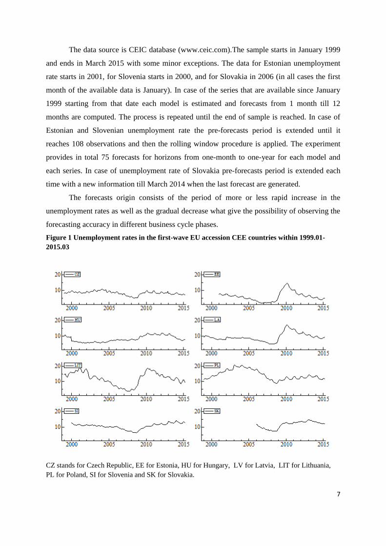
Figure 1 Unemployment rates in the first-wave EU accession CEE countries within 1999.01-

2015.03

CZ stands for Czech Republic, EE for Estonia, HU for Hungary, LV for Latvia, LIT for Lithuania,

PL for Poland, SI for Slovenia and SK for Slovakia.

8

The calculations and graphics are done in OxMetrics STAMP7 [Koopman, Harvey,

Doornik and Shephard 2006, Doornik and Hendry 2005].

Figure 1 shows how unemployment rates changes within the sample period. There is

no single tendency for the unemployment rates in the region at that time, but some common

features are recognizable. At the beginning of the sample some unemployment rates are

increasing and some decreasing. Starting from 2001 the unemployment rates in the region are

decreasing (with Hungarian rate as the exception). There is also a visible change in all series

as they start to increase sharply in the beginning or the mid of 2008 and start to decrease in

the mid 2010 (with the exception of Slovenia). Zooming it the single series behave

differently, some having huge differences between the lowest and the highest point. In the

whole sample the highest unemployment rate was observed in Poland in March 2003 and the

lowest in Estonia in December 2006. The common feature is the dynamic asymmetry which is

observable in all series: the decrease in unemployment rates is rather gradual, whereas the

increase is very steep.

Empirical results

The comparative performance of a rolling forecast experiment is presented in three

steps. In the first one an out-of-sample test of forecast accuracy for the whole forecasts origin

is shown. Then we compare the forecasts errors in two cases: increase and decrease in the

series. In the third step, the errors are depicted together with the series in order to illustrate in

which periods we observe the biggest and the lowest errors.

We report comparative performance of the rolling forecasts in the models used in the

study and described earlier. Tables 1 presents the different forecasting errors for each series

whereby: tlt

y

~ is the l-ahead forecast for a given model, the Mean Error (ME) is obtained as

an average of forecasts errors, tltt yy

~ , the Mean Square Forecast Error (MSFE) is

calculated as square root of averages of 2)~(tltt yy

, and the Mean Absolute Percentage

Error, MAPE, is obtained as an average of %100*/~ttltt yyy

. These errors are reported for

1-month and 1-year horizon.

9

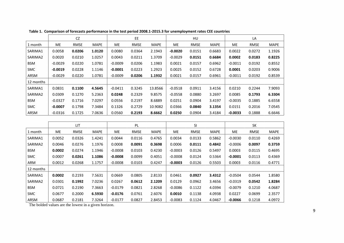
Table 1. Comparison of forecasts performance in the test period 2008.1-2015.3 for unemployment rates CEE countries

CZ EE HU LA

1 month ME RMSE MAPE ME RMSE MAPE ME RMSE MAPE ME RMSE MAPE

SARIMA1 0.0058 0.0206 1.0120 0.0080 0.0364 2.1943 -0.0020 0.0151 0.6683 0.0022 0.0272 1.1926

SARIMA2 0.0020 0.0210 1.0257 0.0043 0.0211 1.3709 -0.0029 0.0151 0.6684 0.0002 0.0183 0.8225

BSM -0.0029 0.0220 1.0781 -0.0009 0.0206 1.1983 0.0021 0.0157 0.6962 -0.0011 0.0192 0.8552

SMC -0.0019 0.0228 1.1146 -0.0001 0.0223 1.2923 0.0025 0.0152 0.6728 0.0001 0.0203 0.9006

ARSM -0.0029 0.0220 1.0781 -0.0009 0.0206 1.1932 0.0021 0.0157 0.6961 -0.0011 0.0192 0.8539

12 months

SARIMA1 0.0831 0.1100 4.5645 -0.0411 0.3245 13.8566 -0.0518 0.0911 3.4156 0.0210 0.2244 7.9093

SARIMA2 0.0309 0.1270 5.2363 0.0248 0.2329 9.8575 -0.0558 0.0880 3.2697 0.0085 0.1793 6.3304

BSM -0.0327 0.1716 7.0297 0.0556 0.2197 8.6889 0.0251 0.0904 3.4197 -0.0035 0.1885 6.6558

SMC -0.0007 0.1798 7.3484 0.1326 0.2729 10.9082 0.0366 0.0840 3.1354 0.0151 0.2016 7.0545

ARSM -0.0316 0.1725 7.0636 0.0560 0.2193 8.6662 0.0250 0.0904 3.4184 -0.0033 0.1888 6.6646

LIT PL SI SK

1 month ME RMSE MAPE ME RMSE MAPE ME RMSE MAPE ME RMSE MAPE

SARIMA1 0.0052 0.0326 1.4241 0.0044 0.0116 0.4765 0.0034 0.0133 0.5862 -0.0030 0.0110 0.4269

SARIMA2 0.0046 0.0276 1.1976 0.0008 0.0091 0.3698 0.0006 0.0111 0.4842 -0.0006 0.0097 0.3759

BSM 0.0002 0.0274 1.1946 -0.0008 0.0103 0.4230 -0.0003 0.0126 0.5497 0.0003 0.0115 0.4695

SMC 0.0007 0.0261 1.1086 -0.0008 0.0099 0.4051 -0.0008 0.0124 0.5364 -0.0001 0.0113 0.4369

ARM 0.0012 0.0268 1.1757 -0.0008 0.0103 0.4247 -0.0003 0.0126 0.5503 0.0003 0.0116 0.4771

12 months

SARIMA1 0.0002 0.2193 7.5631 0.0669 0.0805 2.8133 0.0461 0.0927 3.4312 -0.0504 0.0544 1.8580

SARIMA2 0.0301 0.1992 7.0236 0.0267 0.0612 2.1209 0.0129 0.0962 3.4656 -0.0319 0.0542 1.8284

BSM 0.0721 0.2190 7.3663 -0.0179 0.0821 2.8268 -0.0086 0.1122 4.0394 -0.0079 0.1210 4.0687

SMC 0.0677 0.2000 6.5930 -0.0176 0.0761 2.6076 0.0010 0.1138 4.0938 0.0227 0.0699 2.3577

ARSM 0.0687 0.2181 7.3264 -0.0177 0.0827 2.8453 -0.0083 0.1124 4.0467 -0.0066 0.1218 4.0972 The bolded values are the lowest in a given horizon.

10

In most cases the lowest forecasts errors are obtained from the same model for 1

month and 12 months horizon. The average difference between forecasting errors from

different models are rather small. In terms of considered forecasting errors, the greatest

accuracy is provided by one of the seasonal ARIMA models (for CZ, LA, PL, SI and SK for

both horizons, whereas for HU for 1 month horizon). On aggregate the seasonal ARIMA

models outperform unobserved component models. The empirical evidence speaks strongly

against BSM model as it is the only one which is outperformed by other models for all series.

There is a trade-off between a Mean Error and the Mean Square Forecast Error or Mean

Absolute Percentage Error: the lowest forecasts’ bias measured by Mean Error is observed

for the models that have higher forecasts’ variability.

In the next step the forecasts origin is divided into two subsamples depending on

increase or decrease (or remaining at the same level) of unemployment rates. The formerly

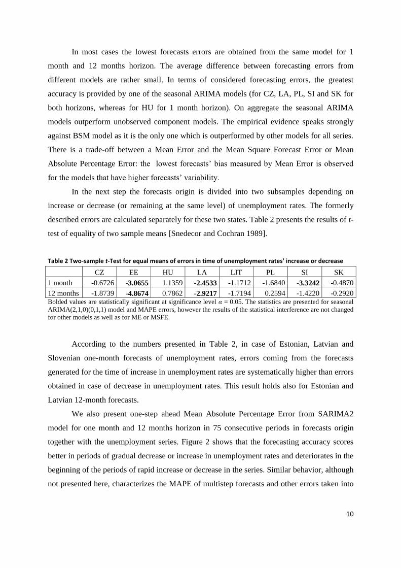
described errors are calculated separately for these two states. Table 2 presents the results of t-

test of equality of two sample means [Snedecor and Cochran 1989].

Table 2 Two-sample t-Test for equal means of errors in time of unemployment rates’ increase or decrease

CZ EE HU LA LIT PL SI SK

1 month -0.6726 -3.0655 1.1359 -2.4533 -1.1712 -1.6840 -3.3242 -0.4870

12 months -1.8739 -4.8674 0.7862 -2.9217 -1.7194 0.2594 -1.4220 -0.2920 Bolded values are statistically significant at significance level α = 0.05. The statistics are presented for seasonal

ARIMA(2,1,0)(0,1,1) model and MAPE errors, however the results of the statistical interference are not changed

for other models as well as for ME or MSFE.

According to the numbers presented in Table 2, in case of Estonian, Latvian and

Slovenian one-month forecasts of unemployment rates, errors coming from the forecasts

generated for the time of increase in unemployment rates are systematically higher than errors

obtained in case of decrease in unemployment rates. This result holds also for Estonian and

Latvian 12-month forecasts.

We also present one-step ahead Mean Absolute Percentage Error from SARIMA2

model for one month and 12 months horizon in 75 consecutive periods in forecasts origin

together with the unemployment series. Figure 2 shows that the forecasting accuracy scores

better in periods of gradual decrease or increase in unemployment rates and deteriorates in the

beginning of the periods of rapid increase or decrease in the series. Similar behavior, although

not presented here, characterizes the MAPE of multistep forecasts and other errors taken into

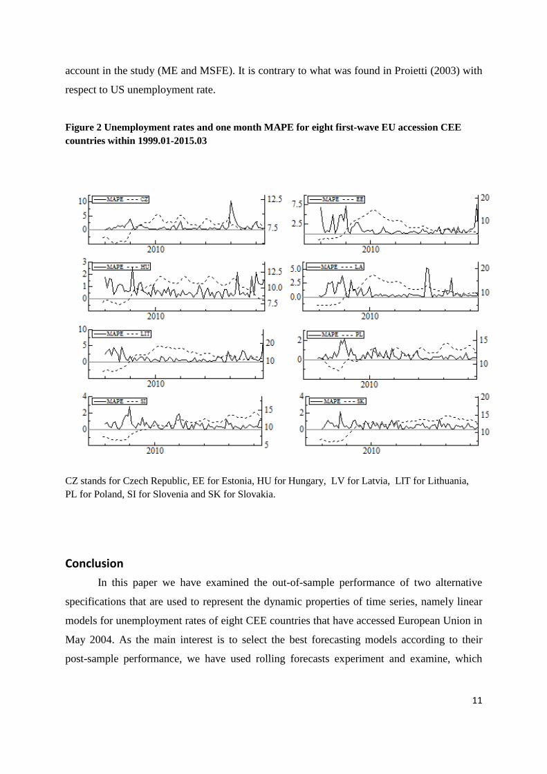
11

account in the study (ME and MSFE). It is contrary to what was found in Proietti (2003) with

respect to US unemployment rate.

Figure 2 Unemployment rates and one month MAPE for eight first-wave EU accession CEE

countries within 1999.01-2015.03

CZ stands for Czech Republic, EE for Estonia, HU for Hungary, LV for Latvia, LIT for Lithuania,

PL for Poland, SI for Slovenia and SK for Slovakia.

Conclusion

In this paper we have examined the out-of-sample performance of two alternative

specifications that are used to represent the dynamic properties of time series, namely linear

models for unemployment rates of eight CEE countries that have accessed European Union in

May 2004. As the main interest is to select the best forecasting models according to their

post-sample performance, we have used rolling forecasts experiment and examine, which

12

model generated the best forecasts. Starting in January 1999 and ending in March 2015 our

sample consists of the periods of decrease and increase in unemployment rates.

We find that for the monthly data in majority of cases seasonal ARIMA models

perform better than unobserved component models considered in the study. The forecasting

ability across different series is surprisingly differential. Generally speaking ARIMA models

prove to be a very useful forecasting tool, both for 1 month and 12 months horizon. Only for

two series in the sample, the Estonian and the Hungarian unemployment rates, the structural

time series models give better forecasts.

When periods of increases and decreases in the unemployment rates are considered

separately, forecasting errors for these two states are significantly different only in three

cases. Last but not least the forecasting accuracy deteriorates in periods of rapid upward and

downward movement and improves in periods of gradual change in the unemployment rates.

References:

Altissimo, F. and G.L. Violante, 2001. “The Non-Linear Dynamics of Output and Un-

employment in the U.S.”, Journal of Applied Econometrics 16: 461-486.

Będowska-Sójka, B., 2015. “Unemployment Rate Forecasts. The Evidence from the Baltic

States”, Eastern European Economics 53: 57-67.

Caner, M. and B.E. Hansen, 2001. “Threshold Autoregression with a Unit Root”, Econo-

metrica 69: 1555-1596.

Doornik, J.A., and D.F. Hendry, 2005. Empirical Econometric Modelling. PcGiveTM

11,

Timberlake Consultants, London.

Harvey, A.C., 1989. “Forecasting Structural Time Series Models and the Kalman Filter”,

Cambridge: Cambridge University Press.

Koop, G. S. and M. Potter, 1999. “Dynamic Asymmetries in U.S. Unemployment”, Journal of

Business and Economic Statistics 17 (3): 298-312.

Koopman, S.J., A.C. Harvey, J.A. Doornik, and N. Shephard. 2006. Structural Time Series

Analyser and Modeller and Predictor STAMP 7, Timberlake Consultants, London.

Marcellino, M. 2002, “Instability and non-linearity in the EMU”, Discussion Paper No. 3312,

Centre for Economic Policy Research.

Milas, C. and P.Rothman. 2005. "Multivariate STAR Unemployment Rate Forecasts,"

Econometrics 0502010, EconWPA.

13

Montgomery, A. L., V, Zarnowitz, R. S. Tsay, and G.C. Tiao. 1998. “Forecasting the U.S.

Unemployment Rate”, Journal of the American Statistical Association 93, no. 442: 478-493.

Neftci, S.N. 1984. “Are Economic Time Series Asymmetric Over the Business Cycle?”

Journal of Political Economy 92, 307-328.

Proietti, T., 2003. “Forecasting the US unemployment rate”, Computational Statistics and

Data Analysis 42: 451-476.

Skalin, J., and T. Teräsvirta, 2002. “Modeling asymmetries and moving equilibria in

unemployment rates”, Macroeconomic Dynamics 6: 202-241.

Snedecor, G.W., and W.G. Cochran, 1989. “Statistical Methods”, Eighth Edition, Iowa State

University Press.

Stock, J.H., and M.W. Watson, 1999. "Business cycle fluctuations in us macroeconomic time

series, in: Taylor, J. B. , M., Woodford (ed.)" Handbook of Macroeconomics”, volume 1: 3-

64, Elsevier.

Teräsvirta, T., D. van Dijk, , and M. C. Medeiros, 2005, “Smooth transition autoregressions,

neural networks, and linear models in forecasting macroeconomic time series: A

reexamination”, International Journal of Forecasting 21, 755-774.