package ‘bnsp’ - the comprehensive r archive network · package ‘bnsp’ september 27, 2018...

Package ‘BNSP’September 27, 2018

Title Bayesian Non- And Semi-Parametric Model Fitting

Version 2.0.8

Date 2018-09-27

Author Georgios Papageorgiou

Maintainer Georgios Papageorgiou <[email protected]>

Description Markov chain Monte Carlo algorithms for non- and semi-parametric models: 1. Dirichlet process mixtures & 2. spike-slab for variable selection in mean/variance regression models.

Depends R (>= 3.1.0)

Imports coda, ggplot2, plot3D, threejs, gridExtra, cubature, Formula,plyr,mgcv

LinkingTo cubature

Suggests mvtnorm, np

License GPL (>= 2)

URL http://www.bbk.ac.uk/ems/faculty/papageorgiou/BNSP

NeedsCompilation yes

Repository CRAN

Date/Publication 2018-09-27 09:10:03 UTC

R topics documented:BNSP-package . . . . . . . . . . . . . . . . . . . . . . . . . . . . . . . . . . . . . . . 2dpmj . . . . . . . . . . . . . . . . . . . . . . . . . . . . . . . . . . . . . . . . . . . . . 3mvrm . . . . . . . . . . . . . . . . . . . . . . . . . . . . . . . . . . . . . . . . . . . . 10mvrm2mcmc . . . . . . . . . . . . . . . . . . . . . . . . . . . . . . . . . . . . . . . . 13plot.mvrm . . . . . . . . . . . . . . . . . . . . . . . . . . . . . . . . . . . . . . . . . . 14predict.mvrm . . . . . . . . . . . . . . . . . . . . . . . . . . . . . . . . . . . . . . . . 15print.mvrm . . . . . . . . . . . . . . . . . . . . . . . . . . . . . . . . . . . . . . . . . 16s . . . . . . . . . . . . . . . . . . . . . . . . . . . . . . . . . . . . . . . . . . . . . . . 17simD . . . . . . . . . . . . . . . . . . . . . . . . . . . . . . . . . . . . . . . . . . . . . 18sm . . . . . . . . . . . . . . . . . . . . . . . . . . . . . . . . . . . . . . . . . . . . . . 19

1

http://www.bbk.ac.uk/ems/faculty/papageorgiou/BNSP

2 BNSP-package

summary.mvrm . . . . . . . . . . . . . . . . . . . . . . . . . . . . . . . . . . . . . . . 20te . . . . . . . . . . . . . . . . . . . . . . . . . . . . . . . . . . . . . . . . . . . . . . 21ti . . . . . . . . . . . . . . . . . . . . . . . . . . . . . . . . . . . . . . . . . . . . . . . 22

Index 24

BNSP-package Bayesian non- and semi-parametric model fitting

Description

Markov chain Monte Carlo algorithms for non- and semi-parametric models: 1. Dirichlet processmixture models with function dpmj and 2. spike-slab variable selection in mean/variance regressionmodels with function mvrm.

Details

Package: BNSPType: PackageVersion: 2.0.7Date: 2018-09-27License: GPL (>=2)

This program is free software; you can redistribute it and/or modify it under the terms of the GNUGeneral Public License as published by the Free Software Foundation; either version 2 of the Li-cense, or (at your option) any later version.

This program is distributed in the hope that it will be useful, but WITHOUT ANY WARRANTY;without even the implied warranty of MERCHANTABILITY or FITNESS FOR A PARTICULARPURPOSE. See the GNU General Public License for more details.

For details on the GNU General Public License see http://www.gnu.org/copyleft/gpl.htmlor write to the Free Software Foundation, Inc., 51 Franklin Street, Fifth Floor, Boston, MA 02110-1301, USA.

Acknowledgments

This work was partly supported by the Medical Research Council grant number G09018401.

Author(s)

Georgios Papageorgiou (2014)

Maintainer: Georgios Papageorgiou <[email protected]>

References

Papageorgiou, G. (2018). Bayesian density regression for discrete outcomes. arXiv:1603.09706v3[stat.ME].

http://www.gnu.org/copyleft/gpl.html

dpmj 3

Papageorgiou, G. (2018). BNSP: an R Package for Fitting Bayesian Semiparametric RegressionModels and Variable Selection. arXiv:1804.10939 [stat.OT]

Papageorgiou, G., Richardson, S. and Best, N. (2015). Bayesian nonparametric models for spa-tially indexed data of mixed type. Journal of the Royal Statistical Society: Series B (StatisticalMethodology), 77:973-999.

dpmj Dirichlet process mixtures of joint models

Description

Fits Dirichlet process mixtures of joint response-covariate models, where the covariates are of mixedtype while the discrete responses are represented utilizing continuous latent variables. See ‘Details’section for a full model description and Papageorgiou (2018) for all technical details.

Usage

dpmj(formula, Fcdf, data, offset, sampler = "truncated", Xpred, offsetPred,StorageDir, ncomp, sweeps, burn, thin = 1, seed, H, Hdf, d, D,Alpha.xi, Beta.xi, Alpha.alpha, Beta.alpha, Trunc.alpha, ...)

Arguments

formula a formula defining the response and the covariates e.g. y ~ x.

Fcdf a description of the kernel of the response variable. Currently five options aresupported: 1. "poisson", 2. "negative binomial", 3. "generalized poisson", 4."binomial" and 5. "beta binomial". The first three kernels are used for countdata analysis, where the third kernel allows for both over- and under-dispersionrelative to the Poisson distribution. The last two kernels are used for binomialdata analysis. See ‘Details’ section for some of the kernel details.

data an optional data frame, list or environment (or object coercible by ‘as.data.frame’to a data frame) containing the variables in the model. If not found in ‘data’, thevariables are taken from ‘environment(formula)’.

offset this can be used to specify an a priori known component to be included in themodel. This should be ‘NULL’ or a numeric vector of length equal to the samplesize. One ‘offset’ term can be included in the formula, and if more are required,their sum should be used.

sampler the MCMC algorithm to be utilized. The two options are sampler = "slice"which implements a slice sampler (Walker, 2007; Papaspiliopoulos, 2008) andsampler = "truncated" which proceeds by truncating the countable mixtureat ncomp components (see argument ncomp).

Xpred an optional design matrix the rows of which include the values of the covariatesx for which the conditional distribution of Y |x,D (where D denotes the data)is calculated. These are treated as ‘new’ covariates i.e. they do not contributeto the likelihood. The matrix shouldn’t include a column of 1’s. NA’s can beincluded to obtain averaged effects.

4 dpmj

offsetPred the offset term associated with the new covariates Xpred. It is of dimensionone i.e. the same offset term is used for all rows of Xpred. If Fcdf is one of"poisson" or "negative binomial" or "generalized poisson", then offsetPred isthe Poisson offset term. If Fcdf is one of "binomial" or "beta binomial", thenoffsetPred is the number of Binomial trials. If offsetPred is missing, it istaken to be the mean of offset, rounded to the nearest integer.

StorageDir a directory to store files with the posterior samples of models parameters andother quantities of interest. If a directory is not provided, files are created in thecurrent directory and removed when the sampler completes.

ncomp number of mixture components. It defines where the countable mixture of den-sities [in (1) below] is truncated. Even if sampler="slice" is chosen, ncompneeds to be specified as it is used in the initialization process.

sweeps total number of posterior samples, including those discarded in burn-in period(see argument burn) and those discarded by the thinning process (see argumentthin).

burn length of burn-in period.

thin thinning parameter.

seed optional seed for the random generator.

H optional scale matrix of the Wishart-like prior assigned to the restricted covari-ance matrices Σ∗h. See ‘Details’ section.

Hdf optional degrees of freedom of the prior Wishart-like prior assigned to the re-stricted covariance matrices Σ∗h. See ‘Details’ section.

d optional prior mean of the mean vector µh. See ‘Details’ section.

D optional prior covariance matrix of the mean vector µh. See ‘Details’ section.

Alpha.xi an optional parameter that depends on the specified Fcdf argument.

1. If Fcdf = "poisson", this argument is parameter αξ of the prior of thePoisson rate: ξ ∼ Gamma(αξ, βξ).

2. If Fcdf = "negative binomial", this argument is a two-dimensional vec-tor that includes parametersα1ξ andα2ξ of the priors: ξ1 ∼Gamma(α1ξ, β1ξ)and ξ2 ∼ Gamma(α2ξ, β2ξ), where ξ1 and ξ2 are the two parameters of theNegative Binomial pmf.

3. If Fcdf = "generalized poisson", this argument is a two-dimensionalvector that includes parametersα1ξ andα2ξ of the priors: ξ1 ∼Gamma(α1ξ, β1ξ)and ξ2 ∼ N(α2ξ, β2ξ)I[ξ2 ∈ Rξ2 ], where ξ1 and ξ2 are the two parametersof the Generalized Poisson pmf. Parameter ξ2 is restricted in the rangeRξ2 = (0.05,∞) as it is a dispersion parameter.

4. If Fcdf = "binomial", this argument is parameter αξ of the prior of theBinomial probability: ξ ∼ Beta(αξ, βξ).

5. If Fcdf = "beta binomial", this argument is a two-dimensional vectorthat includes parameters α1ξ and α2ξ of the priors: ξ1 ∼ Gamma(α1ξ, β1ξ)and ξ2 ∼ Gamma(α2ξ, β2ξ), where ξ1 and ξ2 are the two parameters of theBeta Binomial pmf.

See ‘Details’ section.

Beta.xi an optional parameter that depends on the specified family.

dpmj 5

1. If Fcdf = "poisson", this argument is parameter βξ of the prior of thePoisson rate: ξ ∼ Gamma(αξ, βξ).

2. If Fcdf = "negative binomial", this argument is a two-dimensional vec-tor that includes parameters β1ξ and β2ξ of the priors: ξ1 ∼Gamma(α1ξ, β1ξ)and ξ2 ∼ Gamma(α2ξ, β2ξ), where ξ1 and ξ2 are the two parameters of theNegative Binomial pmf.

3. If Fcdf = "generalized poisson", this argument is a two-dimensionalvector that includes parameters β1ξ and β2ξ of the priors: ξ1 ∼Gamma(α1ξ, β1ξ)and ξ2 ∼ Normal(α2ξ, β2ξ)I[ξ2 ∈ Rξ2 ], where ξ1 and ξ2 are the two pa-rameters of the Generalized Poisson pmf. Parameter ξ2 is restricted in therange Rξ2 = (0.05,∞) as it is a dispersion parameter. Note that β2ξ is astandard deviation.

4. If Fcdf = "binomial", this argument is parameter βξ of the prior of theBinomial probability: ξ ∼ Beta(αξ, βξ).

5. If Fcdf = "beta binomial", this argument is a two-dimensional vectorthat includes parameters β1ξ and β2ξ of the priors: ξ1 ∼ Gamma(α1ξ, β1ξ)and ξ2 ∼ Gamma(α2ξ, β2ξ), where ξ1 and ξ2 are the two parameters of theBeta Binomial pmf.

See ‘Details’ section.

Alpha.alpha optional shape parameter αα of the Gamma prior assigned to the concentrationparameter α. See ‘Details’ section.

Beta.alpha optional rate parameter βα of the Gamma prior assigned to concentration pa-rameter α. See ‘Details’ section.

Trunc.alpha optional truncation point cα of the Gamma prior assigned to concentration pa-rameter α. See ‘Details’ section.

... Other options that will be ignored.

Details

Function dpmj returns samples from the posterior distributions of the parameters of the model:

f(yi, xi) =

∞∑h=1

πhf(yi, xi|θh), (1)

where yi is a univariate discrete response, xi is a p-dimensional vector of mixed type covariates, andπh, h ≥ 1, are obtained according to Sethuraman’s (1994) stick-breaking construction: π1 = v1,and for l ≥ 2, πl = vl

∏l−1j=1(1− vj), where vk are iid samples vk ∼Beta (1, α), k ≥ 1.

Let Z denote a discrete variable (response or covariate). It is represented as discretized version of acontinuous latent variable Z∗. Observed discrete Z and continuous latent variable Z∗ are connectedby:

z = q ⇐⇒ cq−1 < z∗ < cq, q = 0, 1, 2, . . . ,

where the cut-points are obtained as: c−1 = −∞, while for q ≥ 0, cq = cq(λ) = Φ−1{F (q;λ)}.Here Φ(.) is the cumulative distribution function (cdf) of a standard normal variable andF () denotesan appropriate cdf. Further, latent variables are assumed to independently follow a N(0, 1) distri-bution, where the mean and variance are restricted to be zero and one as they are non-identifiableby the data. Choices for F () are described next.

6 dpmj

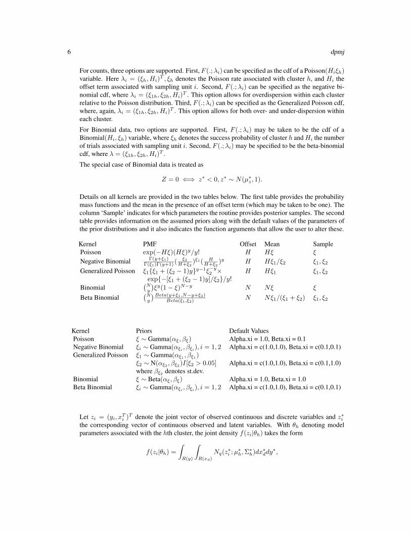
For counts, three options are supported. First, F (.;λi) can be specified as the cdf of a Poisson(Hiξh)variable. Here λi = (ξh, Hi)

T , ξh denotes the Poisson rate associated with cluster h, and Hi theoffset term associated with sampling unit i. Second, F (.;λi) can be specified as the negative bi-nomial cdf, where λi = (ξ1h, ξ2h, Hi)

T . This option allows for overdispersion within each clusterrelative to the Poisson distribution. Third, F (.;λi) can be specified as the Generalized Poisson cdf,where, again, λi = (ξ1h, ξ2h, Hi)

T . This option allows for both over- and under-dispersion withineach cluster.

For Binomial data, two options are supported. First, F (.;λi) may be taken to be the cdf of aBinomial(Hi, ξh) variable, where ξh denotes the success probability of cluster h andHi the numberof trials associated with sampling unit i. Second, F (.;λi) may be specified to be the beta-binomialcdf, where λ = (ξ1h, ξ2h, Hi)

T .

The special case of Binomial data is treated as

Z = 0 ⇐⇒ z∗ < 0, z∗ ∼ N(µ∗z, 1).

Details on all kernels are provided in the two tables below. The first table provides the probabilitymass functions and the mean in the presence of an offset term (which may be taken to be one). Thecolumn ‘Sample’ indicates for which parameters the routine provides posterior samples. The secondtable provides information on the assumed priors along with the default values of the parameters ofthe prior distributions and it also indicates the function arguments that allow the user to alter these.

Kernel PMF Offset Mean SamplePoisson exp(−Hξ)(Hξ)y/y! H Hξ ξ

Negative Binomial Γ(y+ξ1)Γ(ξ1)Γ(y+1) ( ξ2

H+ξ2)ξ1( H

H+ξ2)y H Hξ1/ξ2 ξ1, ξ2

Generalized Poisson ξ1{ξ1 + (ξ2 − 1)y}y−1ξ−y2 × H Hξ1 ξ1, ξ2exp{−[ξ1 + (ξ2 − 1)y]/ξ2}/y!

Binomial(Ny

)ξy(1− ξ)N−y N Nξ ξ

Beta Binomial(Ny

)Beta(y+ξ1,N−y+ξ2)Beta(ξ1,ξ2) N Nξ1/(ξ1 + ξ2) ξ1, ξ2

Kernel Priors Default ValuesPoisson ξ ∼ Gamma(αξ, βξ) Alpha.xi = 1.0, Beta.xi = 0.1Negative Binomial ξi ∼ Gamma(αξi , βξi), i = 1, 2 Alpha.xi = c(1.0,1.0), Beta.xi = c(0.1,0.1)Generalized Poisson ξ1 ∼ Gamma(αξ1 , βξ1)

ξ2 ∼ N(αξ2 , βξ2)I[ξ2 > 0.05] Alpha.xi = c(1.0,1.0), Beta.xi = c(0.1,1.0)where βξ2 denotes st.dev.

Binomial ξ ∼ Beta(αξ, βξ) Alpha.xi = 1.0, Beta.xi = 1.0Beta Binomial ξi ∼ Gamma(αξi , βξi), i = 1, 2 Alpha.xi = c(1.0,1.0), Beta.xi = c(0.1,0.1)

Let zi = (yi, xTi )T denote the joint vector of observed continuous and discrete variables and z∗i

the corresponding vector of continuous observed and latent variables. With θh denoting modelparameters associated with the hth cluster, the joint density f(zi|θh) takes the form

f(zi|θh) =

∫R(y)

∫R(xd)

Nq(z∗i ;µ∗h,Σ

∗h)dx∗ddy

∗,

dpmj 7

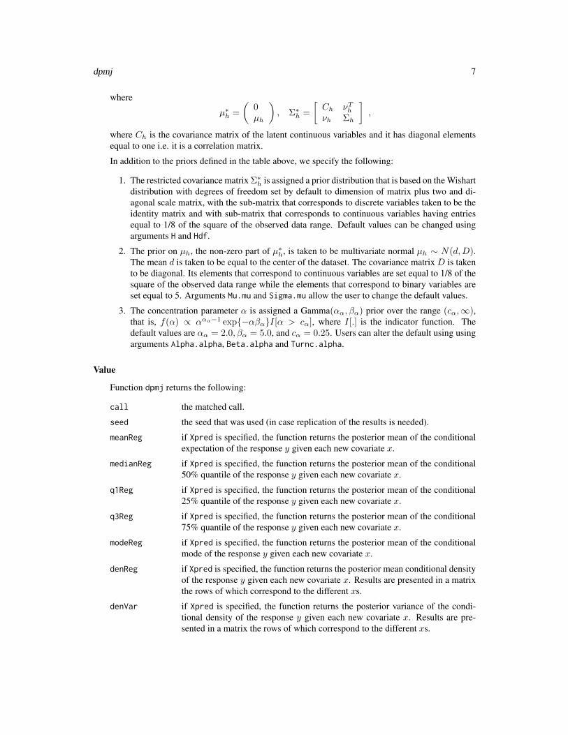
where

µ∗h =

(0µh

), Σ∗h =

[Ch νThνh Σh

],

where Ch is the covariance matrix of the latent continuous variables and it has diagonal elementsequal to one i.e. it is a correlation matrix.

In addition to the priors defined in the table above, we specify the following:

1. The restricted covariance matrix Σ∗h is assigned a prior distribution that is based on the Wishartdistribution with degrees of freedom set by default to dimension of matrix plus two and di-agonal scale matrix, with the sub-matrix that corresponds to discrete variables taken to be theidentity matrix and with sub-matrix that corresponds to continuous variables having entriesequal to 1/8 of the square of the observed data range. Default values can be changed usingarguments H and Hdf.

2. The prior on µh, the non-zero part of µ∗h, is taken to be multivariate normal µh ∼ N(d,D).The mean d is taken to be equal to the center of the dataset. The covariance matrix D is takento be diagonal. Its elements that correspond to continuous variables are set equal to 1/8 of thesquare of the observed data range while the elements that correspond to binary variables areset equal to 5. Arguments Mu.mu and Sigma.mu allow the user to change the default values.

3. The concentration parameter α is assigned a Gamma(αα, βα) prior over the range (cα,∞),that is, f(α) ∝ ααα−1 exp{−αβα}I[α > cα], where I[.] is the indicator function. Thedefault values are αα = 2.0, βα = 5.0, and cα = 0.25. Users can alter the default using usingarguments Alpha.alpha, Beta.alpha and Turnc.alpha.

Value

Function dpmj returns the following:

call the matched call.

seed the seed that was used (in case replication of the results is needed).

meanReg if Xpred is specified, the function returns the posterior mean of the conditionalexpectation of the response y given each new covariate x.

medianReg if Xpred is specified, the function returns the posterior mean of the conditional50% quantile of the response y given each new covariate x.

q1Reg if Xpred is specified, the function returns the posterior mean of the conditional25% quantile of the response y given each new covariate x.

q3Reg if Xpred is specified, the function returns the posterior mean of the conditional75% quantile of the response y given each new covariate x.

modeReg if Xpred is specified, the function returns the posterior mean of the conditionalmode of the response y given each new covariate x.

denReg if Xpred is specified, the function returns the posterior mean conditional densityof the response y given each new covariate x. Results are presented in a matrixthe rows of which correspond to the different xs.

denVar if Xpred is specified, the function returns the posterior variance of the condi-tional density of the response y given each new covariate x. Results are pre-sented in a matrix the rows of which correspond to the different xs.

8 dpmj

Further, function dpmj creates files where the posterior samples are written. These files are (withall file names preceded by ‘BNSP.’):

alpha.txt this file contains samples from the posterior of the concentration parameters α.The file is arranged in (sweeps-burn)/thin lines and one column, each lineincluding one posterior sample.

compAlloc.txt this file contains the allocations to clusters obtained during posterior sampling.It consists of (sweeps-burn)/thin lines, that represent the posterior samples,and n columns, that represent the sampling units. Clusters are represented byintegers ranging from 0 to ncomp-1.

MeanReg.txt this file contains the conditional means of the response y given covariates x ob-tained during posterior sampling. The rows represent the (sweeps-burn)/thinposterior samples. The columns represent the various covariate values x forwhich the means are obtained.

MedianReg.txt this file contains the 50% conditional quantile of the response y given covariatesx obtained during posterior sampling. The rows represent the (sweeps-burn)/thinposterior samples. The columns represent the various covariate values x forwhich the medians are obtained.

muh.txt this file contains samples from the posteriors of the p-dimensional mean vectorsµh, h = 1, 2, . . .,ncomp. The file is arranged in ((sweeps-burn)/thin)*ncomplines and p columns. In more detail, sweeps create ncomp lines representingsamples µ(sw)

h , h = 1, . . . ,ncomp, where superscript sw represents a particularsweep. The elements of µ(sw)

h are written in the columns of the file.nmembers.txt this file contains (sweeps-burn)/thin lines and ncomp columns, where the

lines represent posterior samples while the columns represent the componentsor clusters. The entries represent the number of sampling units allocated to eachcomponent.

Q05Reg.txt this file contains the 5% conditional quantile of the response y given covariates xobtained during posterior sampling. The rows represent the (sweeps-burn)/thinposterior samples. The columns represent the various covariate values x forwhich the quantiles are obtained.

Q10Reg.txt as above, for the 10% conditional quantile.Q15Reg.txt as above, for the 15% conditional quantile.Q20Reg.txt as above, for the 20% conditional quantile.Q25Reg.txt as above, for the 25% conditional quantile.Q75Reg.txt as above, for the 75% conditional quantile.Q80Reg.txt as above, for the 80% conditional quantile.Q85Reg.txt as above, for the 85% conditional quantile.Q90Reg.txt as above, for the 90% conditional quantile.Q95Reg.txt as above, for the 95% conditional quantile.Sigmah.txt this file contains samples from the posteriors of the q × q restricted covariance

matrices Σ∗h, h = 1, 2, . . . ,ncomp. The file is arranged in ((sweeps-burn)/thin)*ncomplines and q2 columns. In more detail, sweeps create ncomp lines representingsamples Σ

(sw)h , h = 1, . . . ,ncomp, where superscript sw represents a particular

sweep. The elements of Σ(sw)h are written in the columns of the file.

dpmj 9

xih.txt this file contains samples from the posteriors of parameters ξh, h = 1, 2, . . . ,ncomp.The file is arranged in ((sweeps-burn)/thin)*ncomp lines and one or twocolumns, depending on the number of parameters in the selected Fcdf. Sweepswrite in the file ncomp lines representing samples ξ(sw)

h , h = 1, . . . ,ncomp,where superscript sw represents a particular sweep.

Updated.txt this file contains (sweeps-burn)/thin lines with the number of componentsupdated at each iteration of the sampler (relevant for slice sampling).

Author(s)

Georgios Papageorgiou <[email protected]>

References

Consul, P. C. & Famoye, G. C. (1992). Generalized Poisson regression model. Communications inStatistics - Theory and Methods, 1992, 89-109.

Papageorgiou, G. (2018). Bayesian density regression for discrete outcomes. arXiv:1603.09706v3[stat.ME].

Papaspiliopoulos, O. (2008). A note on posterior sampling from Dirichlet mixture models. Techni-cal report, University of Warwick.

Sethuraman, J. (1994). A constructive definition of Dirichlet priors. Statistica Sinica, 4, 639-650.

Walker, S. G. (2007). Sampling the Dirichlet mixture model with slices. Communications in Statis-tics Simulation and Computation, 36(1), 45-54.

Examples

#Bayesian nonparametric joint model with binomial response Y and one predictor Xdata(simD)pred<-seq(with(simD,min(X))+0.1,with(simD,max(X))-0.1,length.out=30)npred<-length(pred)# fit1 and fit2 define the same model but with different numbers of# components and posterior samplesfit1 <- dpmj(cbind(Y,(E-Y))~X, Fcdf="binomial", data=simD, ncomp=10, sweeps=20,

burn=10, sampler="truncated", Xpred=pred, offsetPred=30)fit2 <- dpmj(cbind(Y,(E-Y))~X, Fcdf="binomial", data=simD, ncomp=50, sweeps=5000,

burn=1000, sampler="truncated", Xpred=pred, offsetPred=30)plot(with(simD,X),with(simD,Y)/with(simD,E))lines(pred,fit2$medianReg/30,col=3,lwd=2)# with discrete covariatesimD<-data.frame(simD,Xd=sample(c(0,1),300,replace=TRUE))pred<-c(0,1)fit3 <- dpmj(cbind(Y,(E-Y))~Xd, Fcdf="binomial", data=simD, ncomp=10, sweeps=20,

burn=10, sampler="truncated", Xpred=pred, offsetPred=30)

10 mvrm

mvrm Bayesian models for normally distributed responses and semiparamet-ric mean and variance regression models

Description

MCMC for normally distributed responses with additive model for the mean and variance functionsachieved via spike-slab prior for variable selection. See ‘Details’ section for a full description ofthe model.

Usage

mvrm(formula,data,sweeps,burn=0,thin=1,seed,StorageDir,c.betaPrior="IG(0.5,0.5*n)",c.alphaPrior="IG(1.1,1.1)",pi.muPrior="Beta(1,1)",pi.sigmaPrior="Beta(1,1)",sigmaPrior="HN(2)",...)

Arguments

formula a formula defining the response and the covariates in the mean and variancemodels e.g. y ~ x | z or for smooth effects y ~ sm(x) | sm(z). Thepackage uses the extended formula notation, where on the right of ~ we definetwo models: on the right of | is the mean model and on the left is the variancemodel.

data data frame.

sweeps total number of posterior samples, including those discarded in burn-in period(see argument burn) and those discarded by the thinning process (see argumentthin).

burn length of burn-in period.

thin thinning parameter.

seed optional seed for the random generator.

StorageDir a required directory to store files with the posterior samples of models parame-ters.

c.betaPrior The parameters of the inverse Gamma prior of cβ . The default is "IG(0.5,0.5*n)",that is, an inverse Gamma with parameters 1/2 and n/2, where n is the samplesize.

c.alphaPrior The parameters of the inverse Gamma prior of cα. The default is "IG(1.1,1.1)".

pi.muPrior The parameters of the Beta prior of πµ. The default is "Beta(1,1)".

pi.sigmaPrior The parameters of the Beta prior of πσ . The default is "Beta(1,1)".

sigmaPrior The prior of σ2. The default is "HN(2)", a half-normal with variance equal totwo, that is |σ| ∼ N(0, 2). Inverse Gamma prior is also available.

... Other options that will be ignored.

mvrm 11

Details

Function mvrm returns samples from the posterior distributions of the parameters of a regressionmodel with normally distributed responses and mean and variance functions modeled in terms ofcovariates. For instance, in the presence of two covariates in the mean model (u1, u2) and two inthe variance model (w1, w2), we may choose to fit

µu = β0 + β1u1 + fµ(u2),

log(σ2W ) = α0 + α1w1 + fσ(w2),

parametrically modelling the effects of u1 and w1 and non-parametrically the effects of u2 and w2.Smooth functions, such as fµ and fσ , are represented by basis function expansion. For instance

fµ(u2) =∑j

βjφj(u2),

where φ are the basis functions and β are the associated coefficients.

The variance model can equivalently be expressed as

σ2W = exp(α0) exp(α1w1 + fσ(w2)) = σ2 exp(α1w1 + fσ(w2)),

where σ2 = exp(α0). This is the parameterization that we adopt in this implementation.

Positive prior probability that the regression coefficients in the mean model are exactly zero isachieved by defining binary variables γ that take value γ = 1 if the associated coefficient β 6= 0and γ = 0 if β = 0. Indicators δ that take value δ = 1 if the associated coefficient α 6= 0 and δ = 0if α = 0 for the variance function are defined analogously. We note that all coefficients in the meanand variance functions are subject to selection except the intercepts, β0 and α0.

Prior specification:

For the vector of non-zero regression coefficients βγ we specify a g-prior

βγ |cβ , σ2, γ, α, δ ∼ N(0, cβσ2(X̃>γ X̃γ)−1).

where X̃ is a scaled version of design matrix X of the mean model.

For the vector of non-zero regression coefficients αδ we specify a normal prior

αδ|cα, δ ∼ N(0, cαI).

Independent priors are specified for the indicators variables γ and δ as P (γ = 1|πµ) = πµ andP (δ = 1|πσ) = πσ . Further, Beta priors are specified for πµ and πσ

πµ ∼ Beta(cµ, dµ), πσ ∼ Beta(cσ, dσ).

We note that blocks of regression coefficients associated with distinct covariate effects have theirown probability of selection (πµ or πσ) and this probability has its own prior distribution.

Further, we specify inverse Gamma priors for cβ and cα

cβ ∼ IG(aβ , bβ), cα ∼ IG(aα, bα)

Lastly, for σ2 we consider inverse Gamma and half-normal priors

σ2 ∼ IG(aσ, bσ), |σ| ∼ N(0, φ2σ).

12 mvrm

Value

Function mvrm returns the following:

call the matched call.formula model formula.seed the seed that was used (in case replication of the results is needed).data the datasetX the mean model design matrix.Z the variance model design matrix.LG the length of the vector of indicators γ.LD the length of the vector of indicators δ.mcpar the MCMC parameters: length of burn in period, total number of samples, thin-

ning period.nSamples total number of posterior samplesDIR the storage directory

Further, function mvrm creates files where the posterior samples are written. These files are (withall file names preceded by ‘BNSP.’):

alpha.txt contains samples from the posterior of vector α. Rows represent posterior sam-ples and columns represent the regression coefficient, and they are in the sameorder as the columns of design matrix Z.

beta.txt contains samples from the posterior of vector β. Rows represent posterior sam-ples and columns represent the regression coefficients, and they are in the sameorder as the columns of design matrix X.

gamma.txt contains samples from the posterior of the vector of the indicators γ. Rowsrepresent posterior samples and columns represent the indicator variables, andthey are in the same order as the columns of design matrix X.

delta.txt contains samples from the posterior of the vector of the indicators δ. Rowsrepresent posterior samples and columns represent the indicator variables, andthey are in the same order as the columns of design matrix Z.

sigma2.txt contains samples from the posterior of the error variance σ2.cbeta.txt contains samples from the posterior of cβ .calpha.txt contains samples from the posterior of cα.

Author(s)


References

Chan, D., Kohn, R., Nott, D., & Kirby, C. (2006). Locally adaptive semiparametric estimation ofthe mean and variance functions in regression models. Journal of Computational and GraphicalStatistics, 15(4), 915-936.

Papageorgiou, G. (2018). BNSP: an R Package for fitting Bayesian regression models with semi-parametric mean and variance functions. arXiv:1804.10939 [stat.OT]

mvrm2mcmc 13

Examples

# Fit a mean/variance regression model on the cps71 dataset from package nprequire(np)require(ggplot2)data(cps71)model <- logwage ~ sm(age,k=30,bs="rd") | sm(age,k=30,bs="rd")DIR<-getwd()m1<-mvrm(formula=model,data=cps71,sweeps=10,burn=5,thin=1,seed=1,StorageDir=DIR)m2 <- mvrm(formula=model,data=cps71,sweeps=10000,burn=5000,thin=2, seed=1,StorageDir=DIR)#Print information and summarize the modelprint(m2)summary(m2)#Summarize and plot one parameter of interestalpha<-mvrm2mcmc(m2,"alpha")summary(alpha)plot(alpha)#Obtain a plot of a term in the mean modelwagePlotOptions<-list(geom_point(data=cps71,aes(x=age,y=logwage)))plot(x=m2,model="mean",term="sm(age)",plotOptions=wagePlotOptions)#Obtain predictions for new values of the predictor "age"predict(m2,data.frame(age=c(21,65)),interval="credible")

mvrm2mcmc Convert posterior samples from function mvrm into an object of class‘mcmc’

Description

Reads in files where the posterior samples were written and creates an object of class ‘mcmc’ sothat functions like summary and plot from package coda can be used

Usage

mvrm2mcmc(mvrmObj,labels)

Arguments

mvrmObj An object of class ‘mvrm’ as created by a call to function mvrm.

labels The labels of the files to be read in. These can be one or more of: "alpha","beta", "gamma", "delta", "sigma2", "cbeta", "calpha", and they correspond tothe parameters of the model that a call to functions mvrm fits.

Value

An object of class ‘mcmc’ that holds the samples from the posterior of the selected parameter.

14 plot.mvrm

Author(s)


See Also

mvrm

Examples

#see \code{mvrm} example

plot.mvrm Creates plots of terms in the mean and/or variance models

Description

This function plots estimated terms that appear in the mean and variance models.

Usage

## S3 method for class 'mvrm'plot(x,model="mean",term,intercept=TRUE,grid=30,centre=mean,quantiles=c(0.1, 0.9),static=TRUE,centreEffects=FALSE,plotOptions=list(), ...)

Arguments

x an object of class ‘mvrm’ as generated by function mvrm.model one of "mean", "stdev", or "both", specifying which model to be visualized.term the term in the selected model to be plotted.intercept specifies if an intercept should be included in the calculations.grid the length of the grid on which the term will be evaluated.centre a description of how the centre of the posterior should be measured. Usually

mean or median.quantiles the quantiles to be used when plotting credible regions. Plots without credible

intervals may be obtained by setting this argument to NULL.static relevant for 3D plots only. If static=TRUE then plot.mvrm calls function

ribbon3D from package plot3D to create the plot. If static=FALSE then plot.mvrmcalls function scatterplot3js from package threejs to create the plot.

centreEffects if TRUE then the effects in the mean functions are centred around zero overthe range of the predictor while the effects in the variance function are scaledaround one.

plotOptions for plots of univariate smooth terms or for plots of bivariate smooth terms whereone of the two covariates is discrete, this is a list of plot elements to give toggplot. For smooths of bivariate continuous covariates, this is a list of plotelements to give to ribbon3D (if static=FALSE) or to scatterplot3js (ifstatic=TRUE).

... other arguments.

predict.mvrm 15

Details

Use this function to obtain predictions.

Value

Predictions along with credible/pediction intervals

Author(s)


See Also

mvrm

Examples


predict.mvrm Model predictions

Description

Provides predictions and posterior credible/prediction intervals for given feature vectors.

Usage

## S3 method for class 'mvrm'predict(object, newdata, interval = c("none", "credible", "prediction"),

level = 0.95, nSamples = 100, ...)

Arguments

object an object of class "mvrm", usually a result of a call to mvrm.

newdata data frame of feature vectors to obtain predictions for. If newdata is missing,the function will use the feature vectors in the data frame used to fit the mvrmobject.

interval type of interval calculation.

level tolerance level.

nSamples number of samples to obtain from the posterior predictive distribution (for eachsweep of the MCMC). Only relevant for "prediction intervals".


16 print.mvrm

Details

The function returns predictions of new responses or the means of the responses for given featurevectors. Predictions for new responses or the means of new responses are the same. However, thetwo differ in the associated level of uncertainty: response predictions are associated with wider(prediction) intervals than mean response predictions. To obtain prediction intervals (for new re-sponses) the function samples from the normal distributions with means and variances as sampledduring the MCMC run.

Value

Predictions for given covariate/feature vectors.

Author(s)


See Also

mvrm

Examples


print.mvrm Prints an mvrm fit

Description

Provides basic information from an mvrm fit.

Usage

## S3 method for class 'mvrm'print(x, digits = 5, ...)

Arguments

x an object of class "mvrm", usually a result of a call to mvrm.

digits the number of significant digits to use when printing.


Details

The function prints information about mvrm fits.

s 17

Value

The function provides a matched call, the number of posterior samples obtained and marginal in-clusion probabilities of the terms in the mean and variance models.

Author(s)


See Also

mvrm

Examples


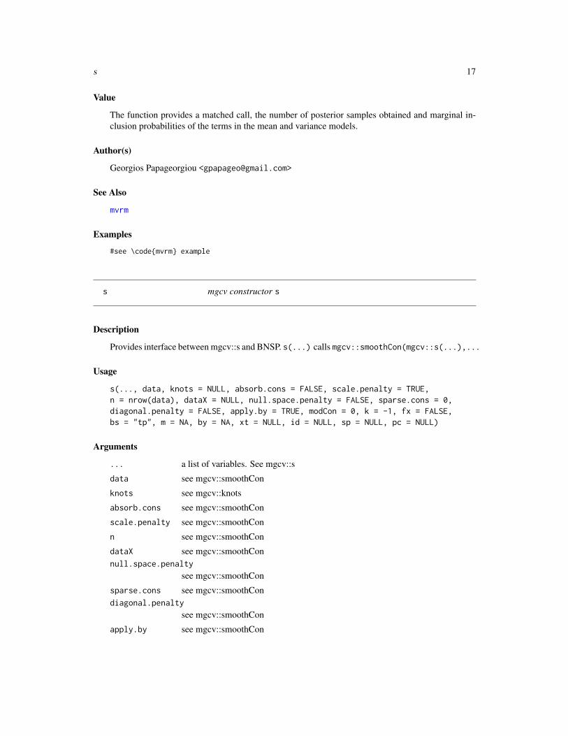
s mgcv constructor s

Description

Provides interface between mgcv::s and BNSP. s(...) calls mgcv::smoothCon(mgcv::s(...),...

Usage

s(..., data, knots = NULL, absorb.cons = FALSE, scale.penalty = TRUE,n = nrow(data), dataX = NULL, null.space.penalty = FALSE, sparse.cons = 0,diagonal.penalty = FALSE, apply.by = TRUE, modCon = 0, k = -1, fx = FALSE,bs = "tp", m = NA, by = NA, xt = NULL, id = NULL, sp = NULL, pc = NULL)

Arguments

... a list of variables. See mgcv::s

data see mgcv::smoothCon

knots see mgcv::knots

absorb.cons see mgcv::smoothCon

scale.penalty see mgcv::smoothCon

n see mgcv::smoothCon

dataX see mgcv::smoothConnull.space.penalty

see mgcv::smoothCon

sparse.cons see mgcv::smoothCondiagonal.penalty

see mgcv::smoothCon

apply.by see mgcv::smoothCon

18 simD

modCon see mgcv::smoothCon

k see mgcv::s

fx see mgcv::s

bs see mgcv::s

m see mgcv::s

by see mgcv::s

xt see mgcv::s

id see mgcv::s

sp see mgcv::s

pc see mgcv::s

Details

The most relevant arguments for BNSP users are the list of variables ..., knots, absorb.cons, bs,and by.

Value

A design matrix that specifies a smooth term in a model.

Author(s)


simD Simulated dataset

Description

Just a simulated dataset to illustrate the model. The success probability and the covariate have anon-linear relationship.

Usage

data(simD)

Format

A data frame with 300 independent observations. Three numerical vectors contain information on

Y number of successes.

E number of trials.

X explanatory variable.

sm 19

sm Smooth terms in mvrm formulae

Description

Function used to define smooth effects in the mean and variance formulae of function mvrm. Thefunction is used internally to construct the design matrices.

Usage

sm(...,k=10,knots=NULL,bs="rd")

Arguments

... one or two covariates that the smooth term is a function of. If two covariates areused, they may be both continuous or one continuous and one discrete. Discretevariables should be defined as factor in the data argument of the calling mvrmfunction.

k the number of knots to be utilized in the basis function expansion.

knots the knots to be utilized in the basis function expansion.

bs a two letter character indicating the basis functions to be used. Currently, theoptions are "rd" that specifies radial basis functions and is available for uni-variate and bivariate smooths, and "pl" that specifies thin plate splines that areavailable for univariate smooths.

Details

Use this function within calls to function mvrm to specify smooth terms in the mean and/or variancefunction of the regression model.

Univariate radial basis functions with q basis functions or q − 1 knots are defined by

B1 ={φ1(u) = u, φ2(u) = ||u− ξ1||2 log

(||u− ξ1||2

), . . . , φq(u) = ||u− ξq−1||2 log

(||u− ξq−1||2

)},

where ||u|| denotes the Euclidean norm of u and ξ1, . . . , ξq−1 are the knots that are chosen as thequantiles of the observed values of explanatory variable u, with ξ1 = min(ui), ξq−1 = max(ui)and the remaining knots chosen as equally spaced quantiles between ξ1 and ξq−1.

Thin plate splines are defined by

B2 = {φ1(u) = u, φ2(u) = (u− ξ1)+, . . . , φq(u) = (u− ξq)+} ,

where (a)+ = max(a, 0).

Radial basis functions for bivariate smooths are defined by

B3 ={u1, u2, φ3(u) = ||u− ξ1||2 log

(||u− ξ1||2

), . . . , φq(u) = ||u− ξq−1||2 log

(||u− ξq−1||2

)}.

20 summary.mvrm

Value

Specifies the design matrices of an mvrm call

Author(s)


See Also

mvrm

Examples


summary.mvrm Summary of an mvrm fit

Description

Provides basic information from an mvrm fit.

Usage

## S3 method for class 'mvrm'summary(object, nModels = 5, digits = 5, ...)

Arguments

object an object of class "mvrm", usually a result of a call to mvrm.

nModels integer number of models with the highest posterior probability to be displayed.

digits the number of significant digits to use when printing.


Details

Use this function to summarize mvrm fits.

Value

The functions provides a detailed description of the specified model and priors. In addition, thefunction provides information about the Markov chain ran (length, burn-in, thinning) and the folderwhere the files with posterior samples are stored. Lastly, the function provides the mean posteriorand null deviance and the mean/variance models visited most often during posterior sampling.

te 21

Author(s)


See Also

mvrm

Examples


te mgcv constructor te

Description

Provides interface between mgcv::te and BNSP. te(...) calls mgcv::smoothCon(mgcv::te(...),...

Usage

te(..., data, knots = NULL, absorb.cons = FALSE, scale.penalty = TRUE,n = nrow(data), dataX = NULL, null.space.penalty = FALSE, sparse.cons = 0,diagonal.penalty = FALSE, apply.by = TRUE, modCon = 0, k = NA, bs = "cr",m = NA, d = NA, by = NA, fx = FALSE, np = TRUE, xt = NULL, id = NULL,sp = NULL, pc = NULL)

Arguments

... a list of variables. See mgcv::te







see mgcv::smoothCon


see mgcv::smoothCon



k see mgcv::te

22 ti

bs see mgcv::te

m see mgcv::te

d see mgcv::te

by see mgcv::te

fx see mgcv::te

np see mgcv::te

xt see mgcv::te

id see mgcv::te

sp see mgcv::te

pc see mgcv::te

Details


Value


Author(s)


ti mgcv constructor ti

Description

Provides interface between mgcv::ti and BNSP. ti(...) calls mgcv::smoothCon(mgcv::ti(...),...

Usage

ti(..., data, knots = NULL, absorb.cons = FALSE, scale.penalty = TRUE,n = nrow(data), dataX = NULL, null.space.penalty = FALSE, sparse.cons = 0,diagonal.penalty = FALSE, apply.by = TRUE, modCon = 0, k = NA, bs = "cr",m = NA, d = NA, by = NA, fx = FALSE, np = TRUE, xt = NULL, id = NULL,sp = NULL, mc = NULL, pc = NULL)

ti 23

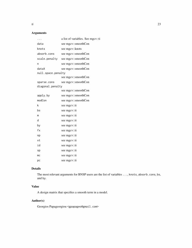
Arguments

... a list of variables. See mgcv::ti







see mgcv::smoothCon


see mgcv::smoothCon



k see mgcv::ti

bs see mgcv::ti

m see mgcv::ti

d see mgcv::ti

by see mgcv::ti

fx see mgcv::ti

np see mgcv::ti

xt see mgcv::ti

id see mgcv::ti

sp see mgcv::ti

mc see mgcv::ti

pc see mgcv::ti

Details


Value


Author(s)


Index

∗Topic clusterdpmj, 3

∗Topic datasetssimD, 18

∗Topic modelssm, 19

∗Topic nonparametricdpmj, 3mvrm, 10

∗Topic regressionmvrm, 10sm, 19

∗Topic smoothmvrm, 10sm, 19

BNSP (BNSP-package), 2BNSP-package, 2

dpmj, 3

mvrm, 10, 14–17, 20, 21mvrm2mcmc, 13

plot.mvrm, 14predict.mvrm, 15print.mvrm, 16

s, 17simD, 18sm, 19summary.mvrm, 20

te, 21ti, 22

24

package ‘bnsp’ - the comprehensive r archive network · package ‘bnsp’ september 27, 2018...

Documents