Outdoor Auralization

Evaluation of a road simulation model

M A R J A G U S T I N

Master of Science Thesis Stockholm, Sweden 2010

Outdoor Auralization

Evaluation of a road simulation model

M A R J A G U S T I N

Master’s Thesis in Electro Acoustics (30 ECTS credits) at the School of Media Technology Royal Institute of Technology year 2010 Supervisor was Svante Granqvist Examiner was Sten Ternström TRITA-CSC-E 2010:002 ISRN-KTH/CSC/E--10/002--SE ISSN-1653-5715 Royal Institute of Technology School of Computer Science and Communication KTH CSC SE-100 44 Stockholm, Sweden URL: www.csc.kth.se

Outdoor AuralizationEvaluation of a Road Simulation Model

Abstract

A simulation model for road traffic has been evaluated on behalf of The Interactive Institute in Kista. The model consists of simulations of vehicle passages that are put together to simulate a traffic flow. Selected parts of the simulation program have been implemented and the model has been evaluated in three different listening tests, to find if the database of vehicle sounds can be reduced. The first test established if it is possible to distinguish a difference between a traffic flow where all vehicles travel in the same lane and a traffic flow where both driving directions get their own lane. In the second test, the loudness of the engine noise in the simulated vehicle sounds was varied, to find how this affected the perceived realism. The third test established how large differences in velocity are possible to detect. The tested velocities were in the range of 30-70 km/h.

The results from the tests show that the difference between a one lane and a two lane traffic flow is not distinct. The loudness of the engine noise can be varied, but not to a large extent, as the perceived realism then rather quickly decreases. Within the range of tested velocities, it was found a difference of 8 km/h is possible to detect. It was also shown that the ability to detect this difference increases at higher velocities.

Auralisering i utomhusmiljö Utvärdering av en trafiksimuleringsmodell

Sammanfattning

En simuleringsmodell för biltrafik har utvärderats på uppdrag av Interaktiva Institutet i Kista. Modellen bygger på simuleringar av olika bilpassager, vilka sammanfogas i ett program för att simulera en trafikerad väg. Utvalda delar av simuleringsprogrammet har implementerats och modellen har sedan utvärderats i tre lyssnartester i syfte att utreda om databasen modellen bygger på går att reducera. Det första testet har undersökt huruvida det är möjligt att höra skillnad på ett trafikflöde där alla bilar åker i samma körfält och ett flöde där de båda färdriktningarna får sitt eget körfält. I det andra testet varierades styrkan på motorljudet i de simulerade billjuden för att se hur det påverkade den upplevda realismen. I ett tredje test utreddes hur stora skillnader i hastighet som är möjliga att upptäcka. De hastigheter som testades låg mellan 30-70 km/h.

Resultaten från testerna visar att skillnaden mellan ett enfiligt och ett tvåfiligt trafikflöde inte är distinkt. Ljudstyrkan på motorljudet går att variera något men vid större ändringar sjunker den upplevda realismen relativt fort. Inom det testade spannet av hastigheter visade det sig att det går att uppleva en skillnad i hastighet på 8 km/h. Det visade sig även att förmågan att detektera denna skillnad ökar vid högre hastigheter.

Preface

As part of the research project LISTEN, this thesis has been written on behalf of The Interactive Institute. The LISTEN project is a collaboration between The Interactive Institute, Stockholm University, The Royal Institute of Technology, Chalmers University of Technology and the University College of Arts, Crafts and Design.

The thesis has been supervised by PhD Svante Granqvist at The Speech, Music and Hearing department at The Royal Institute of Technology. Supervisor at The Interactive Institute was Peter Lundén. The listening tests have been additionally supervised by Senior Lecturer Mats E. Nilsson at Stockholm University.

I would like to thank all the people involved in this thesis, including all participants in the listening tests.

Marja Gustin

Stockholm, January 2010

Table of Contents

1. Introduction 1

1.1 Background 1

1.1.1 Auralization 1

1.1.2 The LISTEN project 2

1.2 Problem statement 3

1.3 Aims and objectives 3

1.4 Delimitation 3

2. Theory 4

2.1 Simulating traffic noise 4

2.2 Modelling of the vehicle sounds 4

3. Method 7

3.1 Pure Data prototyping 7

3.1.1 The prototype 7

3.2 Test preparations 8

3.2.1 Preparing the stimuli 9

3.2.2 Test subjects 9

3.2.3 Test equipment and calibration 9

3.3 The distance test 10

3.3.1 Test design 10

3.3.2 The test 11

3.4 The dynamics test 12

3.4.1 Visual Sort and Rate 12

3.4.2 The test 13

3.5 The speed test 13

3.5.1 Visual Sort and Rate 13

3.5.2 The test 13

4. Results 16

4.1 The distance test 16

4.2 The dynamics test 17

4.3 The speed test 17

5. Discussion 21

6. Conclusions 22

7. Future Work 23

8. Bibliography 24

9. Appendices 25

1. Introduction

When planning the building of an urban environment it can be of interest knowing what it will sound like in this space. With the use of noise predicting measures, calculations can be made to try to establish the characteristics and loudness of the environmental sound at a given listening position. Conveying the acquired data could however be problematic, as it requires a level of knowledge in the person interpreting the results. If the environmental sound instead was simulated, making it possible to play back the results to a listener, the data would probably be easier to understand.

Noise predicting and preventing measures in existing as well as in non-existing environments are fairly large fields of research. The market consists of several software applications for interior acoustics prediction, as well as a number of consulting companies designing or re-designing the sound in specific environments. Most of these simulate sound in indoor environments, such as rooms, churches or subway platforms. Predicting sound in a closed space where the architectural structure is known, as well as the objects and materials forming the space, mean a calculation model can be used built on this known data. In an outdoor environment this prediction gets more complex, as the propagating sound waves not only have more space to travel in, but also are affected by changing temperature and wind as well as unpredictable interfering objects, such as moving vehicles.

Swedish research project LISTEN is focusing on simulating road and railway traffic noise in outdoor environments. The simulated noise will be used in a demonstrating tool, which will make it possible to listen to noise in not-yet-built outdoor environments. This thesis, assigned by LISTEN project partner The Interactive Institute, has consisted of evaluating a model simulating road traffic. Listening tests were performed to find ways of optimising the program simulating the traffic flow, by reducing the database of vehicle sounds it is built on.

As the simulation program was a work in progress, certain functions had to be implemented as part of the thesis to enable the listening tests being performed.

1.1 Background

1.1.1 Auralization

The process of generating signals, and handling and reproducing them is called auralization (Vorländer 2008). Also the perceivable result, such as the simulated sound in a room, is described by this term. Auralization is a technique for creating audible sound files from numerical data, which can be simulated, measured or synthesised (Vorländer 2008). Auralization is analogous to visualisation in the sense that it presents an image of a virtual reality, in this case an audible representation of a three-dimensional space.

Computer models based on geometrical acoustics have been used for simulation of sound in rooms since the late 1960’s (Vorländer 2008). The algorithms mainly calculate the sound field in energy,

1

transition time and the directions of rays. A few of the biggest manufacturers of auralization software today are CATT-acoustic1, Odeon2 and Head acoustics3.

Outdoor auralization is still a quite unexplored field of research, most likely due to the complexity of predicting sound in an outdoor environment.

1.1.2 The LISTEN project

The LISTEN project is a three year research project focusing on developing a demonstration tool, a demonstrator, which simulates noise produced by road and railway traffic (Forssén et al 2009). The demonstrator can be used for assessing different soundscapes, that is, sounds formed or originated by an environment, at the planning stage. Also, it can show how noise prevention measures, such as a noise barrier, will affect the sound (KK-stiftelsen 2009).

The demonstrator is built on simulations of vehicle sounds, created by Jens Forssén at Chalmers University of Technology. The sound files have been optimised for headphone listening by Peter Lundén at The Interactive Institute. The created sound files simulate vehicles travelling on a straight road at different speeds, at different distances from the listener, as well as with or without a noise barrier on the side of the road. Each sound file represents a specific scenario, for instance a vehicle travelling at 50 km/h at 6 metres distance from the listener, with a noise barrier at the road side. This results in a fairly large database of sounds (1500 files at the time of the writing of this report).

The synthesised sounds have been evaluated and compared to real recordings. The listening tests were conducted at The Gösta Ekman Laboratory at Stockholm University. Participants were asked to distinguish a real recording from an auralization of the same recording, as well as assess perceived annoyance, speed and similarity of real and auralized recordings (Forssén et al 2009). The tests showed that high-speed vehicle simulations were perceived as more realistic than lower speed simulations.

To create a first prototype of the demonstrator, the database of sounds was used to generate a fictitious road for binaural listening. This was done by Peter Lundén at The Interactive Institute. The prototype was created in the programming environment Pure Data4, simulating traffic travelling on a straight road. The prototype was able to simulate a traffic flow of vehicles coming from both left and right at a 6 metre distance from the listener. The simulated road was straight with no level differences and no surrounding obstacles affecting the sound. The simulated vehicles were travelling on asphalt, while the listener was standing on a grass surface.

The final demonstrator in the LISTEN project should be able to simulate three scenarios. The first is an outdoor soundscape where a block of flats is directly exposed to road or railway traffic. The second is in an indoor room exposed to traffic noise. The third is an outdoor soundscape at the shielded side of a block of flats (KK-stiftelsen 2009). The listener should be able to choose from different listening positions as well as adding or removing a noise barrier.

2

1 www.catt.se

2 www.odeon.dk

3 http://www.head-acoustics.de/eng/index.htm

4 http://puredata.info

1.2 Problem statement

The demonstrator simulates different scenarios by adding sound files specific for each setting. An increasing number of scenarios leads to an increased sound database, which equals a more complex and power-demanding simulation process. Therefore, it is essential to find ways to make this process more efficient, for instance by trying to reduce the size of the database. If this isn’t possible, it might be necessary to find other ways to simulate traffic noise, for instance by real-time simulation of each vehicle sound.

To be able to evaluate different aspects of the demonstrator, necessary functions were implemented in a simulation program as the first part of this thesis. Three areas of the demonstrator were then evaluated in listening tests. The questions to be answered were the following:

- Is it necessary to have different lanes for traffic moving in opposite directions, or is it possible to simplify the simulation model by having all vehicles travelling in the same lane?

- How loud should the propulsion noise be, that is, the noise generated by the vehicle propulsion mechanisms, in relation to the tyre noise to achieve the highest sense of realism?

- How small differences in speed are possible to detect? Does this difference depend on the speed?

1.3 Aims and objectives

The first part of this thesis has focused on implementing specific prototype functions to meet the criteria specified within the LISTEN project. The second part has focused on performing listening tests on selected prototype functions. The results from the listening tests will be evaluated to find if there are possible ways to make the simulation model more efficient.

1.4 Delimitation

In this thesis, selected parts of the prototype were evaluated. The intention has not been to finalise the prototype itself. The implementations made in the prototype are part of an iterative process trying to establish ways to create different functions in a demonstrator of this sort and they will not necessarily be definitive solutions for the final demonstrator. The listening tests are to be seen as feasibility studies, which can indicate areas where further studies might be relevant.

3

2. Theory

2.1 Simulating traffic noise

To be able to create a model of a vehicle travelling along a fictitious road, several parameters that affect the sound need to be taken into consideration. Below is a list of such parameters and a description of how they apply to this scenario. The list is not complete, but explains some main factors relevant to this project.

Tyre/Road noise (rolling noise). The noise generated by the rolling tyres when they are in contact with the ground.

Propulsion noise. The sound of the vehicle propulsion mechanism, such as the engine noise, air intake, air exhaust, fans, compressors etc. (Forssén et al. 2009).

Temperature and humidity. When modelling the vehicle sounds for the simulation program, average values for temperature and humidity were used (Salomons & Heimann 2004). Effects of refraction, i.e. curved sound paths caused by wind or height varying temperature were not accounted for (Forssén et al. 2009).

Doppler effect. When the source of a periodic sound (and/or the receiver) is in motion relative to the propagating waves, the wave frequency, as measured by the receiver, is different from the source frequency (Mansfield & O’Sullivan 1998). The frequency of the vehicle sound will be higher when the vehicle approaches the listener and lower as it recedes.

Comb filter effect. The effect caused by delayed reflection on the frequency response of a signal is often called a comb filter (Everest & Pohlmann 2009). When a delayed replica of a sound is mixed with the original sound, phasing and flanging effects can occur. These are the results of two signals being out of phase, creating nulls and peaks in the frequency response. The result of interference between sound travelling directly from the source to the receiver and sound reflected from the ground is called the ground effect (Rossing 2007). In this project the ground reflections are modelled for a grass surface (Lundén 2009).

Head Related Transfer Function, HRTF. The generated sound files are encoded for headphone listening, using a head related transfer function. This calculates the sound coming to the left and right ears, accounting for the head and torso influence on the sound. HRTFs from the CIPIC HRTF database have been used (CIPIC Interface Laboratory 2004).

2.2 Modelling of the vehicle sounds The vehicle sounds used in the simulation prototype are created by LISTEN project partner Jens Forssén, Associate Professor at Chalmers University of Technology. The development of the vehicle sounds is based on a model by European project Harmonoise (de Vos, Beuving & Verheijen 2005).

4

The aim of the Harmonoise project is to develop methods for predicting environmental noise levels from road and railway traffic. A source model has been constructed to calculate sound pressure levels of road traffic noise (Jonasson et al. 2004). An overview of how the vehicle sounds are generated is presented below. For a more detailed description of how to model vehicle sounds, see Jonasson et al. (2004), Salomons and Heimann (2004) and Forssén et al. (2009).

When creating a model of the vehicle, each vehicle is represented by two point sources located on a vertical line (Jonasson et al. 2004 & Forssén et al. 2009). The first source is located 0.01 m above the ground and the second is 0.03 m above the ground. The point sources are incoherent and move with constant speed along a line (Salomons & Heimann 2004). The figure shows the geometrical setup, where the source moves along the y-axis from y1 to y2 (fig. 1).

Figure 1. Geometrical setup of a moving point source on the y-axis and the receiver at a fixed position (x,0) on the x-axis. (Salomons & Heimann 2004)

Before creating the point source signals, mono recordings of single vehicles passing at constant speed were analysed (Forssén et al. 2009 & Kaczmarek 2008). The recorded vehicle velocities were 27, 45, 65, 84 and 106 km/h and the vehicle had an otto engine. To create the point source signals, the recorded signals were then reshaped using an inverted approach, in which the effect of spherical spreading, the Doppler effect, the ground effect and the air attenuation were removed from the recorded sounds (Forssén et al. 2009). The remaining signal was then analysed to distinguish propagation noise characteristics from rolling noise characteristics (Lundén 2009).

Using filtered white noise, the resulting signal was then replicated (Lundén 2009). Each of the point sources had a specific sound power with different contributions from the rolling noise and the propulsion noise. 80% of the rolling noise and 20% of the propulsion noise was assigned to the source located 0.01 metres above the ground. 20% of the rolling noise and 80% of the propulsion noise was assigned to the source located 0.03 metres above the ground (for further details of point source modelling see Jonasson 2004).

The propagation effects (air attenuation, ground effect, distance and the Doppler effect) were then modelled using the same tools as in the inversion process (Forssén et al. 2009). A database was generated consisting of vehicles travelling at different speeds, vehicles at different distances from the listener, and vehicles travelling on a road with a noise barrier between the vehicle and the listener. All vehicles were simulated to travel on asphalt, with the listener standing on a grass surface. The road was straight and each vehicle travelled at constant speed with no interfering

5

objects around. The speed simulations ranged from 20-140 km/h in steps of 2 km/h. The distance between the listener and the middle of the road was simulated for 7.5 and 25 metres. The vehicle distance from the listening position is 6, 9, 23.5 and 26.5 metres, enabling a traffic flow where vehicles are travelling in two separate lanes. Each vehicle passage was a monophonic WAV file, 15-second in length.

Finally, the sound files were HRTF-encoded for headphone playback, to replicate the listening position of a listener standing by the side of the road.

6

3. Method

To be able to evaluate parts of the demonstrator, certain functions of the prototype were implemented in the existing Pure Data simulating program. Selected parts of the prototype were then evaluated in three different listening tests. The first was a distance test, which tried to establish if it was possible to distinguish a one-lane traffic simulation from a two-lane simulation. The second was a dynamics test, trying to find a realistic mix between the tyre noise loudness and the propulsion noise loudness, as well as finding out if it is possible to simulate different types of cars by varying this loudness. The third was a speed test, testing how small differences in speed are possible to detect and if these differences vary with speed.

The main reason for evaluating these parts of the prototype was to find out if it is possible to reduce the database of vehicle sounds, enabling a less power-demanding simulation program. If the tests show that a database reduction is not possible, real-time simulation of the vehicle sounds might have to be considered.

3.1 Pure Data prototyping

To be able to evaluate the prototype, certain functions of the prototype had to be implemented. A control panel was also programmed to enable different settings in the prototype to be easily changed.

3.1.1 The prototype

The existing prototype, created by Peter Lundén, was able to load a number of sound files and put them together to simulate a traffic flow. The startup of each vehicle sound was Poisson-distributed to create an uneven flow of traffic, with vehicles coming from both left and right. All vehicles were driving on a 6-metre distance from the listener, meaning that cars were driving in the same lane in opposite directions. Within the scope of this thesis, the following improvements of the prototype were made:

- Scenario Distance: The listener should be able to choose from two different listening positions; 7.5 metres and 25 metres. For each position, vehicles coming from left and right should travel in different lanes. This was done by loading different files for different listening positions, as well as changing the simulation program so that vehicles coming from the left consisted of sound files of vehicles travelling closer than those coming from the right.

Noise barrier: The listener should be able to add a noise barrier. This is done by loading vehicle sounds that contains a noise barrier simulation.

- Memory usage The size of each sound file is 4 MB, and the original prototype loaded all sound files into the memory at start-up. This was changed so that only sound files with a speed around the chosen average speed was loaded into the simulation program.

7

-Start-up When the simulation is started, the simulation process should already be ongoing, to avoid the listener having to wait for the first cars to pass by. This is done by adding 15 seconds of simulation to the start-up process. As all vehicles sounds initially were composed of the same white noise, this start-up change resulted in a comb filter effect, as many vehicles with a similar spectral content interfered with each other. To avoid this, the vehicle sounds were changed by Jens Forssén by varying the noise they were constructed of.

- Control Panel A control panel connecting with the program over Internet protocol UDP (user datagram protocol) was programmed in Pure Data, using the Pure Data command sendOSC (fig. 2). This enables the user to change the listening distance, add a noise screen as well as changing a number of parameters such as the mean speed and the number of vehicle passages per hour. The reason for using a UDP connection was to enable the interface being implemented in another programming language later, connecting with the Pure Data patch over the Internet.

Figure 2. The control panel, enabling the user to set a number of parameters such as distance, noise barrier on or off, mean speed and the number of vehicle passages per hour.

3.2 Test preparations

Before the tests were performed, all test stimuli had to be prepared and calibrated to realistic listening levels. Also, the test equipment had to be calibrated. This was done at the Gösta Ekman

8

Laboratory at Stockholm University, using a Brüel & Kjaer head and torso simulator. A hearing test was also performed on each test subject, to ensure that everyone was of normal hearing.

3.2.1 Preparing the stimuli

For each listening test, a number of stimuli had to be prepared. This was done by creating custom Pure Data patches that loaded different vehicle files, changing them if necessary and saving a pre-defined section of the file (appendix 1). The lengths of the stimuli for the listening tests were assessed in different pilot studies and the listeners often preferred a shorter version of the vehicle passage than what was used in the demonstrator (the original passage was 15 seconds long). The passages used in the speed test were five seconds long, keeping only the middle part of the sound file simulating the actual pass by. The stimuli used in the dynamics test were eight seconds long and the ones used in the distance test were 20 seconds long. The latter could be listened to for as long as the test person wanted, while the other two sets of stimuli had to be listened to in full. By keeping the stimulus shorter, the possibility for the listener to remember an old stimulus while listening to a new one increased.

3.2.2 Test subjects

Twenty-two test subjects participated in the listening tests. Each test subject did all three listening tests in a single session that lasted approximately one hour. 16 males and 6 females born in 1986-1949 participated. The mean age was 28 years and 18 of the participants were KTH students. A hearing test was performed on each test subject using a Madsen Electronics OB 822 Clinical Audiometer, calibrated with hearing level measurements of young people with normal hearing. A deviance of 20 dB from the calibrated hearing threshold was allowed. The frequencies tested were 125, 250, 500, 750, 1000, 1500, 2000, 3000, 4000, 6000 and 8000 Hz. 18 subjects were normal hearing. One subject had a 30 dB deviation on the right ear at 8000 Hz. Another subject had a deviation of 25 dB on the right ear. Two subjects had deviations between 25 and 55 dB on both ears from 3000 Hz to 8000 Hz.

The tests took place at the Speech, Music and Hearing department at KTH. The location made it easy to find KTH students willing to participate, explaining the large number of participants from this group. A lot of the participants were also of similar age. It is possible that the outcome of the tests could be different with a less homogeneous group. The participants did not receive an economic compensation for participating in the tests.

3.2.3 Test equipment and calibration

To run the tests, one Macintosh and one Dell PC were used. Each were connected to an Alesis iO|2 sound card and AKG K-240 headphones. The distance test was running on the Macintosh, the speed and dynamics tests were running on the PC.

The equipment for the listening tests was calibrated with a Brüel & Kjaer head and torso simulator (HATS), model number 4100 (fig. 3). The microphones in the HATS were calibrated with a Brüel & Kjaer pistonphone producing a 1000 Hz pure tone at 94.5 dB. Each computer setup played a 1000 Hz pure tone through the headphones, which were placed on the dummy head. Two people placed the headphones on the dummy head five times each for both test setups. A medium of the ten

9

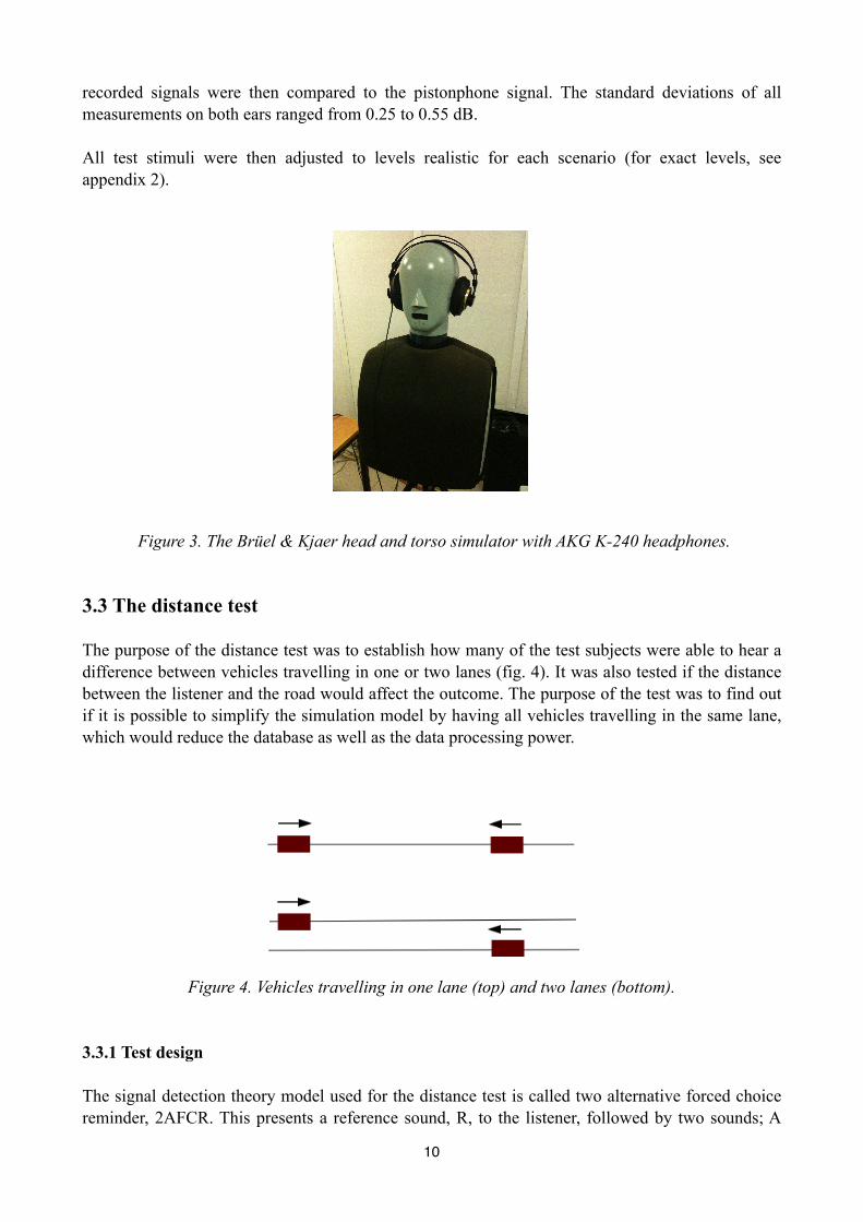
recorded signals were then compared to the pistonphone signal. The standard deviations of all measurements on both ears ranged from 0.25 to 0.55 dB.

All test stimuli were then adjusted to levels realistic for each scenario (for exact levels, see appendix 2).

Figure 3. The Brüel & Kjaer head and torso simulator with AKG K-240 headphones.

3.3 The distance test

The purpose of the distance test was to establish how many of the test subjects were able to hear a difference between vehicles travelling in one or two lanes (fig. 4). It was also tested if the distance between the listener and the road would affect the outcome. The purpose of the test was to find out if it is possible to simplify the simulation model by having all vehicles travelling in the same lane, which would reduce the database as well as the data processing power.

Figure 4. Vehicles travelling in one lane (top) and two lanes (bottom).

3.3.1 Test design

The signal detection theory model used for the distance test is called two alternative forced choice reminder, 2AFCR. This presents a reference sound, R, to the listener, followed by two sounds; A

10

and B. The listener is then asked to select which of A and B is most similar to R. The reference is always the same, while A and B alters. If the reference sound P1 is presented before the two samples

P1 and P2, the two possible sequences are {P1, P1, P2 } and {P1, P2, P1 } (Hautus, van Haut & Lee 2009). In this case, none of the stimuli A and B are identical to the reference R, but instead one of them simulates traffic moving in one lane, just as the reference. This method was chosen as it provides a high level of power for small differences in characteristics (Hautus, van Haut & Lee 2009). The listener has to make a choice each time a new set of stimuli is presented, and the correspondence between the correct response and the listener’s ”forced choice” is of interest (Macmillan & Creelman 2005). The reminder design is good in situations where the discrimination itself is difficult, as the listener in these cases sometimes has trouble remembering what the signal sounds like (Macmillan & Creelman 2005). The reminder design enables the listener to go back and listen to the reference sound several times, making the comparison easier.

3.3.2 The test

The listener was presented with a reference sound, being a simulation where all cars were travelling in the same lane. The listener was told the reference would always be the same for each test. Then, two example sounds were presented; one where the cars were travelling in the same lane and one where each driving direction had its own lane. The question asked was: which of the example sounds is most similar to the reference sound? A clue was also given: in one of the example sounds, the cars are driving on the same type of road as in the reference. The listener was given a feedback response, indicating if the answer was correct or not. A test patch designed in Pure Data by Peter Lundén was used for the test (fig. 5).

Figure 5. The 2AFCR test patch. The listener can listen to each stimulus several times before making a choice. A feedback response is given, indicating if the answer was correct or not.

11

As the vehicle sound database consists of files simulating two listening distances, both distances were tested. In the case where all vehicles were travelling in the same lane, the distance from the listener was 6 metres in the first case and 23.5 metres in the second. When each driving direction had its own lane, the distance was 6 and 9 metres in the first case and 23.5 and 26.5 metres in the second. The possible test sequences were as follows:

Ref. A B

6 m 6 m 6 and 9 m

6 m 6 and 9 m 6m

23.5 m 23.5 m 23.5 and 26.5 m

23.5 m 23.5 and 26.5 m 23.5 m

Table 1. Possible test sequences in the 2AFCR distance test.

Each stimulus was a 20 second long simulation of a traffic flow where the average speed was 78 km/h with the density of 6600 vehicle passages per hour. The listener could listen to each stimulus as many times as preferred, and did not have to listen to each in full. The reference stimulus was always the same, while there were three different recordings of each of the other stimuli. The test files were calibrated to individual sound pressure levels for each type of file (appendix 2).

The chosen test design was 7-13-16, resulting in a confidence interval of 99% (Granqvist 2008). The 7-13-16 design means the test series will be accepted if the listener gets the first seven answers right. The series will also be accepted if the listener gets 12 out of 13 right, or 14 out of 16. Otherwise the listener will have failed the test. However, failing the test does not mean the listener did not hear a difference. The test can only establish whether a difference can be detected.

3.4 The dynamics test

Each vehicle sound is composed of a rolling noise simulation and a propulsion noise simulation. To find if an increase or decrease of the propulsion noise gain can be perceived as more or less realistic, a dynamics test was prepared. In the test, the propulsion noise was varied with a gain of -18 to +18 dB, in steps of 3 dB, while the rolling noise was kept constant. If the test showed that several combinations were rated high, it might be possible to simulate different types of cars by changing the propulsion noise gain.

The vehicle simulation used in the test was a vehicle driving at a 6-metre distance from the listener at 40 km/h. The sound pressure level at the ears of the listener with no propulsion noise gain was 67 dB.

3.4.1 Visual Sort and Rate To establish the perceived realism of different combinations of rolling and propulsion loudness, the visual sort and rate (VSR) method was used. This method uses a graphical representation for each stimulus (Granqvist 2003). By clicking the icon, the stimulus can be listened to. The listener then rates each stimulus by placing the icon along a vertical line. The test was implemented in VSR test

12

environment Visor and the method was chosen as it allows the listener to compare different stimuli as well as rate them according to perceived realism.

3.4.2 The test

Thirteen stimuli with varying propulsion noise gain were prepared. The listener was asked to rate each combination according to perceived realism, by placing each of the 13 stimuli along a vertical axis graded from unreal to real. The instructions were: rate each of these vehicles according to perceived realism. Pilot studies showed that different stimuli could be perceived as being different kinds of vehicles, such as small and large ones, but still be perceived as real. It was decided that the type of car should not be considered, but merely the perceived realism on each individual stimulus. This was conveyed to the listener. The set of stimuli were not calibrated to have equal total loudness, as the loudness was one factor that was of interest in the test. Instead, the total sound pressure level varied for each stimulus.

Every test subject did the test twice, resulting in 44 different test series. The placement on the vertical axis was translated into a number between 0 and 1000 and the mean of all test sets was calculated for each stimulus.

3.5 The speed test

To establish how small differences in speed are detectable, a speed test was performed. The existing database simulates speed in increasing steps of two km/h and the results from the test could offer guidance on whether to increase or decrease these steps.

3.5.1 Visual Sort and Rate

The VSR test method was chosen for the test, implemented in Visor (fig. 6). The reason this method was used is that it not only establishes the smallest detectable change in speed, but also shows if the results vary with velocity.

3.5.2 The test

To find the smallest detectable change in speed, 21 test stimuli were prepared, each stimulus being a five-second-long single vehicle passage. The speed range was 30-70 km/h with an increase of speed in steps of 2 km/h. The listener was instructed to listen to each stimulus and place it along the vertical axis, with the lowest perceived speed at the bottom, the highest at the top and the rest in perceived speed order in between. Each stimulus could be listened to several times.

13

Figure 6. The Visor test set-up. Each stimulus is represented by a box that plays the stimulus when clicked. The icon is then placed along the vertical axis to the left.

Each test subject did the test twice, resulting in 44 different test series. Depending on the placement on the vertical axis, each stimulus received a rating between 0 and 1000. The mean value of all 44 placements of each speed was calculated. Also, the mean of all placements made by participants of normal hearing was calculated, as well as the mean of all test series in which the test subject had listened to 70% or more of the stimuli more than once.

To find how small differences in speed were possible to detect, and if this detectable difference varied with velocity, a paired t-test at a 0.05 significance level was performed (Dalgaard 2008). This test establishes whether the difference between velocity A and velocity B is significant or not with a 95% certainty.

The mean rating, x, for each person’s two placements of each stimulus was calculated. Then, the stimuli were paired and the difference between the placements was calculated for each pair. The first set of pairs were stimuli with a difference in velocity of 2 km/h:

x32 - x30

x34 - x32

.

.

.x70 - x68

14

Then, the difference between pairs with a difference in velocity of 4, 6, 8, 10 and 12 km/h was calculated. For each pair, the average difference, davg, for all 22 test participants placements was calculated:

d1 = x1, 32 - x1, 30

.

.

.d22 = x22, 32 - x22, 30

The standard deviation, sd, of all 22 participants placements was calculated for each pair. To find the t-value, determining if the difference is significant or not, the following formula was used:

t = davg / (sd / √n), n = number of participants

A table of the t distribution was used to find a value for t with n-1 = 21 degrees of freedom on a 5% significance level. The t-value was calculated for each pair to find what difference in speed is possible to detect.

15

4. Results

4.1 The distance test

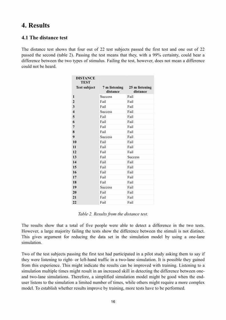
The distance test shows that four out of 22 test subjects passed the first test and one out of 22 passed the second (table 2). Passing the test means that they, with a 99% certainty, could hear a difference between the two types of stimulus. Failing the test, however, does not mean a difference could not be heard.

DISTANCE TEST

Test subject 7 m listening distance

25 m listening distance

12345678910111213141516171819202122

Success FailFail FailFail FailSuccess FailFail FailFail FailFail FailFail FailSuccess FailFail FailFail FailFail FailFail SuccessFail FailFail FailFail FailFail FailFail FailSuccess FailFail FailFail FailFail Fail

Table 2. Results from the distance test.

The results show that a total of five people were able to detect a difference in the two tests. However, a large majority failing the tests show the difference between the stimuli is not distinct. This gives argument for reducing the data set in the simulation model by using a one-lane simulation.

Two of the test subjects passing the first test had participated in a pilot study asking them to say if they were listening to right- or left-hand traffic in a two-lane simulation. It is possible they gained from this experience. This might indicate the results can be improved with training. Listening to a simulation multiple times might result in an increased skill in detecting the difference between one- and two-lane simulations. Therefore, a simplified simulation model might be good when the end-user listens to the simulation a limited number of times, while others might require a more complex model. To establish whether results improve by training, more tests have to be performed.

16

4.2 The dynamics test

The acquired mean values of the 44 listening tests show that a 3 dB gain of the propulsion noise was rated to be most realistic (fig. 7). A larger increase than that results in a rapid decrease in the perceived realism. The quite narrow peak of the plotted curve shows that the loudness of the propulsion noise shouldn’t be varied to a large extent in order to maintain a high level of realism.

fig. 7. The perceived realism of the different test stimuli. The y-axis shows the medium rate for each stimulus, the x-axis shows how much the propulsion loudness was changed for each stimulus.

4.3 The speed test

The average speed rating is illustrated below (fig. 8). Removing the test results by participants with a hearing impairment did not affect any of the results, nor did removing the results by those not listening to 70% or more of the stimuli more than once. Therefore, all 44 test series are included in all calculations. The average values of the highest and lowest speed stimuli will be affected by the restrictions of the scale at the ends.

0

200

400

600

800

−18−15−12 −9 −6 −3 0 3 6 9 12 15 18

Perceived realism

ratin

g

dB

17

Figure 8. The average rating of each speed stimulus.

A possible explanation for the dips in the curve was thought to be the fact that different speed recordings were used when modelling the vehicle sounds. However, the dips do not coincide with this data, so it is possible that they are just a coincidence.

The following diagram shows the average distance of all sets of stimuli pairs in relation to the actual difference in speed (fig. 9).

Figure 9. The average distance for all sets of stimuli pairs. The x-axis shows the actual difference between the compared stimuli in km/h, the y-axis shows the average rated distance for all stimuli.

0

200

400

600

800

1000

30 34 38 42 46 50 54 58 62 66 70

Speed rating - all participants

ratin

g

km/h

0

45

90

135

180

225

2 4 6 8 10 12

Average distance

Ave

rage

rat

ed d

ista

nce

Actual difference (km/h)

18

The results from the t-tests shows that a difference in speed of 8 km/h is possible to detect (fig. 10). For these pairs, all but one has a significant difference in distance. A series with one or two non-significant pairs is accepted, as the non-significant pairs are probably a coincidence.

Figure 10. The average distance between stimulus with a difference in velocity of 8 km/h. All pairs but number 4 has a significant difference in distance.

The test also shows that that the perceived difference gets larger as the velocity increases. The perceived difference for pairs with 10 and 12 km/h differences indicates similar results (fig. 11 and 12).

Figure 11. The average distance between stimulus with a difference in velocity of 10 km/h. All pairs above the line are significant.

0

75

150

225

300

0 2 4 6 8 10 12 14 16 18

Average distance for pairs with an 8 km/h velocity differenceA

vera

ge r

ated

dis

tanc

e

Pair number

Pair1 = 38-302 = 40-323 = 42-344 = 44-365 = 46-386 = 48-407 = 50-428 = 52-449 = 54-46

10 = 56-4811 = 58-5012 = 60-5213 = 62-5414 = 64-5615 = 66-5816 = 68-6017 = 70-62

0

75

150

225

300

0 2 4 6 8 10 12 14 16 18 20

Average distance for pairs with a 10 km/h velocity difference

Ave

rage

rat

ed d

iffer

ence

Pair number

Pair1 = 40-302 = 42-323 = 44-344 = 46-365 = 48-386 = 50-407 = 52-428 = 54-449 = 56-46

10 = 58-4811 = 60-5012 = 62-5213 = 64-5414 = 66-5615 = 68-5816 = 70-60

19

Figure 12. The average distance between stimulus with a difference in velocity of 12 km/h. Pair number 4 is non-significant.

A similar trend can be seen already at 6 km/h (fig. 13). The stimuli above the line are all significant, suggesting that from around 50 km/h and upwards it is possible to detect a difference of 6 km/h.

Figure 13. The average distance between stimulus with a difference in velocity of 6 km/h. All pairs above the line are significant.

0

100

200

300

400

0 3 6 9 12 15

Average distance for pairs with a 12 km/h velocity difference

Ave

rage

rat

ed d

iffer

ence

Pair number

Pair1 = 42-302 = 44-323 = 46-344 = 48-365 = 50-386 = 52-407 = 54-428 = 56-449 = 58-46

10 = 60-4811 = 62-5012 = 64-5213 = 66-5414 = 68-5615 = 70-58

0

75

150

225

300

0 2 4 6 8 10 12 14 16 18 20

Average distance for pairs with a 6 km/h velocity difference

Ave

rage

rat

ed d

iffer

ence

Pair number

Pair1 = 36-302 = 38-323 = 40-344 = 42-365 = 44-386 = 46-407 = 48-428 = 50-449 = 52-46

10 = 54-4811 = 56-5012 = 58-5213 = 60-5414 = 62-5615 = 64-5816 = 66-6017 = 68-6218 = 70-64

20

5. Discussion

The listening tests show it is possible to reduce the database to a large extent. If the existing listening distances are used, it is possible to use a one-lane simulation, reducing the database by half. If more listening distances are added, it might be of interest to establish at what distance a difference between a one- and two-lane simulation could be heard. The simulation model could then use a two-lane simulation for listening distances where a difference can be heard, and a one-lane simulation for other distances.

The outcome of the distance test might have been different if the test participants had been able to do some training prior to the test, for instance by not counting the first five answers. However, the purpose of the test was to find out if an inexperienced listener could detect a difference.

The dynamics test shows the propulsion noise loudness cannot be varied to a large extent, in order to maintain a high level of realism. By varying the loudness of the propulsion noise it is possible to simulate different types of vehicles. This would result in keeping the number of sound files to a minimum, instead of having to generate specific sound files for each specific car simulation.

As the test participants were aware the set of stimuli consisted of simulated vehicles only, it is possible this affected the way the stimuli were ranked. If real vehicle recordings were mixed with the simulated ones, the outcome might have been different. It would also make it possible to compare ratings of real vehicle sounds to simulated ones.

The speed test showed it is possible to detect a difference in speed of 8 km/h. However, at higher velocities this ability increases. In pilot studies made prior to the tests, it seemed the participants picked up a lot of information about the speed from the actual pass by, that is, the moment the vehicle passes the listener’s head. At higher velocities the pass by is faster and more distinct than at lower velocities. This can be a possible explanation to the increased ability to detect changes in velocity at higher speed.

The test participants were told to rank the stimulus according to perceived speed. As the stimuli increased in steps of two, the results were often a straight line of stimuli placed at equal distance from each other. Another way of designing the test is to have unequal steps of increasing velocity. The participants could then be instructed to not only place the stimuli on the axis from slow to fast, but also adjust the distance between each stimulus.

The database consisted of simulations of vehicles with a change in speed in steps of two km/h. No prior tests had been made to motivate this. As the tests showed it is not possible to detect differences in speed at this resolution, it is suggested to decrease the database by reducing the number of velocity simulations. As the ability to detect changes in speed increases as the velocity increases, all speed simulations from 20-140 km/h should be tested to find out how much each part of the database should be reduced.

The tests show it is possible to reduce the database of vehicle sounds. However, for each new scenario, a number of new sound files have to be added. Also, with the existing method used it is not possible for the vehicles to start, stop and change speed. Therefore, real-time simulation of the vehicle sounds might have to be considered. This is discussed within the LISTEN project, but would include further studies of, for instance, vehicle engine noise.

21

6. Conclusions

The results from each test show that the database can be decreased. In the distance test, it is established there is no distinct difference between a one-lane and a two-lane simulation. In the dynamics test, results indicate it is possible to vary the propulsion noise loudness whilst maintaining a high level of realism, enabling different sounding vehicles to be produced without having to add more sound files. The test also establishes the stimulus with a +3 dB gain is rated the highest. The speed test shows that a difference in speed of 8 km/h can be detected for velocities between 30-70 km/h. As the ability to detect changes in speed increases as the velocity increases, the full database has to be tested in order to decide how many velocity simulations can be removed.

With a simulation model built on pre generated sound files, the number of sound files will have to be increased for each new scenario added. Building a model using pre generated sound files also means the simulation program will be more static compared to a real time generated vehicle simulation where vehicles can change speed, start and stop. While the existing simulation program can be made more effective by reducing the database of sound files, for a future application it is suggested that the vehicle sounds are real time simulated.

22

7. Future Work

If more listening distances are added, an adaptive distance test could be designed to find if the ability to distinguish between a one-lane and two-lane simulation increases at closer distances.

By having listeners compare the top rated stimulus in the dynamics test with real recordings of different vehicles, differences in perceived realism between the two categories can be found.

To find out which velocity simulations should be included in the database, tests should be performed on all velocities from 20-140 km/h.

23

8. Bibliography

CIPIC Interface Laboratory (2004). Available: <http://interface.cipic.ucdavis.edu/CIL_html/CIL_HRTF_database.htm>, 2009-10-21

Dalgaard, Peter (2008). Introductory Statistics with R, Second Edition, Springer Science+Business Media, LLC, New York. p. 153

Everest, F. Alton & Pohlmann, Ken (2009). Master Handbook of Acoustics, McGraw-Hill, USA. p. 135

Forssén, Jens, Kaczmarek, Tomasz, Alvarsson, Jesper, Lundén, Peter & Nilsson, Mats E. (2009). Auralization of traffic noise within the LISTEN project - Preliminary results for passenger car pass-by, PDF, p. 1, 2, 6-8

Granqvist, Svante (2003). The Visual Sort and Rate method for perceptual evaluation in listening tests, PDF, Available: <http://www.speech.kth.se/~svante/Thesis/paperI.pdf>, p. 4

Granqvist, Svante (2008). Elektroakustik: Laboration B2, lyssningstest, PDF. Available: <http://www.csc.kth.se/utbildning/kth/kurser/DT2400/ablab.pdf>

Hautus, M.J., van Hout, D, Lee, H.-S (2009). Variants of A Not-A and 2AFC tests: Signal Detection Theory models, Food Quality and Preference 20. p. 222-229

Jonasson, Hans Sandberg, Ulf, van Blokland, Gijsjan, Ejsmont, Jurek, Watts, Greg & Luminari, Marcello (2004). Source modelling of road vehicles, PDF. Available: <http://www.imagine-project.org/bestanden/D09_WP1.1_HAR11TR-041210-SP10.pdf>, p. 2

Kaczmarek, T (2008). Subjective verification of simulation of a vehicle pass-by, PDF. 3136,

KK-stiftelsen (2009). Available: <http://www.kks.se/templates/ProjectPage.aspx?id=13726>, 2009-11-23>

Lundén, Peter (2009). Personal communication.

Macmillan, Neil A., Creelman, C. Douglas (2005). Detection Theory: A User’s Guide (2nd edition). Lawrence Erlbaum Associates Inc. p. 166, 180, 230

Mansfield, Michael & O’Sullivan, Colm (1998). Understanding Physics. Eastergate: John Wiley & Sons Ltd. p. 338-339

Pure Data (2009). Available: <http://puredata.info/>, 2009-10-19

Salomons, Erik & Heimann, Dieter (2004). Description of the Reference model, Deliverable 16 of the Harmonoise project, PDF. Available: <http://www.imagine-project.org/bestanden/ D16_WP2_HAR29TR-041118-TNO10.pdf>- p. 7, 13

Vorländer, Michael (2008). Auralization. Fundamentals of Acoustics, Modelling, Simulation, Algorithms and Acoustic Virtual Reality. Berlin Heidelberg: Springer-Verlag, Preface VII, p. 103

de Vos, Paul, Beuving, Margareet & Verheijen, Edwin (2005). Final Technical Report, Deliverable 4 of the HARMONOISE project, PDF. Available: <http://www.imagine-project.org/bestanden/ D04_WP7_HAR7TR-041213-AEAT04.pdf>, p. 3

24

9. Appendices

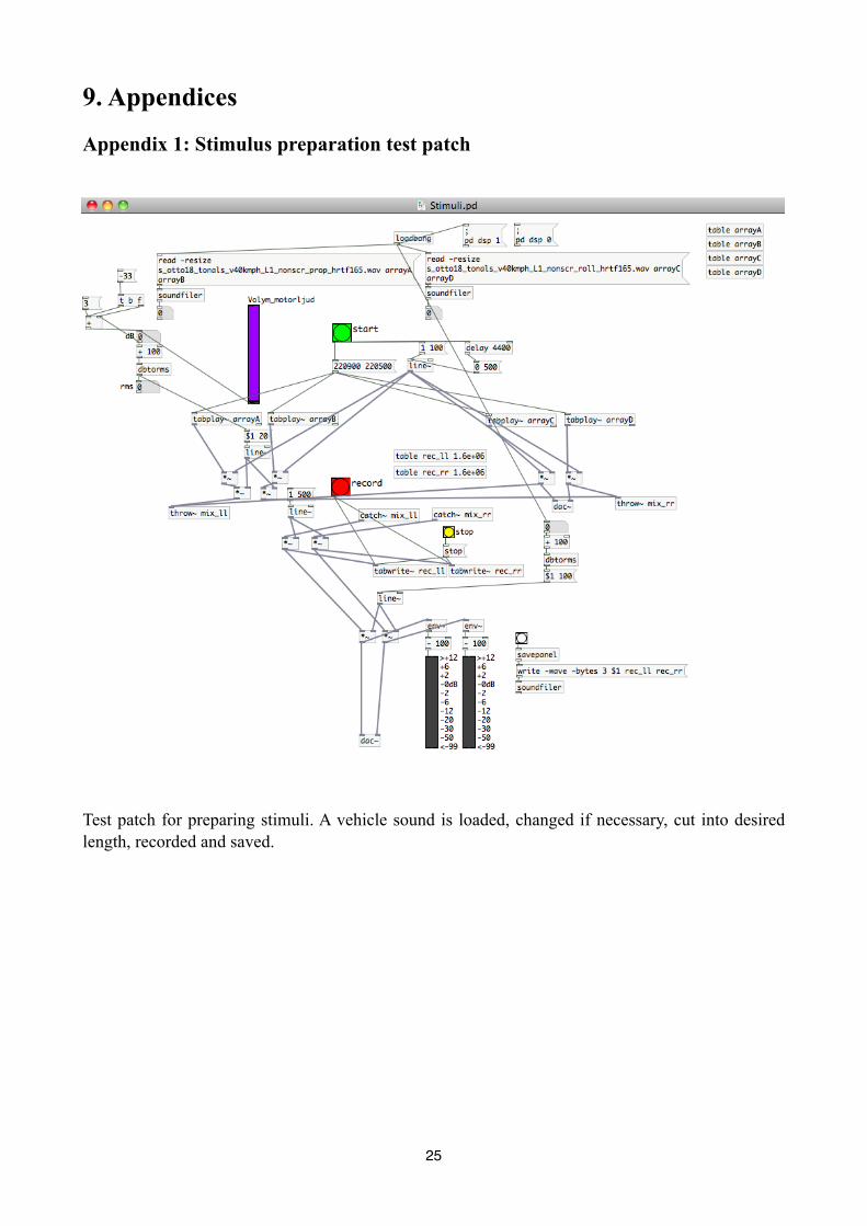
Appendix 1: Stimulus preparation test patch

Test patch for preparing stimuli. A vehicle sound is loaded, changed if necessary, cut into desired length, recorded and saved.

25

Appendix 2: Stimuli playback levels

DISTANCE TEST

Stimulus Average level of total sound file(dBA)

One lane, 6 m 78.36

One lane, 25 m 72.20

Two lanes, 6 and 9 m 75.71

Two lanes, 23.5 and 26.5 m

70.80

SPEED TEST

Stimulus (km/h)

Top level at passage(dBA)

30 64.85

32 65.48

34 65.85

36 66.38

38 66.84

40 67.27

42 67.91

44 68.81

46 68.90

48 69.35

50 69.82

52 70.60

54 71.32

56 71.47

58 72.15

60 73.17

62 73.58

64 73.92

26

SPEED TEST

66 73.86

68 74.50

70 75.05

27

TRITA-CSC-E 2010:002 ISRN-KTH/CSC/E--10/002--SE

ISSN-1653-5715

www.kth.se