1

Guided Multiview Ray Tracing for FastAuralization

Micah Taylor, Anish Chandak, Qi Mo, Christian Lauterbach, Carl Schissler, and Dinesh Manocha,

Abstract—We present a novel method for tuning geometric acoustic simulations based on ray tracing. Our formulation computessound propagation paths from source to receiver and exploits the independence of visibility tests and validation tests todynamically guide the simulation to high accuracy and performance. Our method makes no assumptions of scene layout and canaccount for moving sources, receivers, and geometry. We combine our guidance algorithm with a fast GPU sound propagationsystem for interactive simulation. Our implementation efficiently computes early specular paths and first order diffraction witha multi-view tracing algorithm. We couple our propagation simulation with an audio output system supporting a high orderinterpolation scheme that accounts for attenuation, cross-fading, and delay. The resulting system can render acoustic spacescomposed of thousands of triangles interactively.

Index Terms—Sound propagation, ray tracing, parallelization.

F

1 INTRODUCTION

Auditory displays and sound rendering are frequently usedto enhance the sense of immersion in virtual environmentsand multimedia applications. Aural cues combine withvisual cues to improve realism and the user’s experience.One of the challenges in interactive virtual environments isto perform auralization and visualization at interactive rates,i.e. 30fps or better. Current graphics hardware and algo-rithms make it possible to visually render complex sceneswith millions of primitives at interactive rates. On the otherhand, current auralization methods cannot generate realisticsound effects at interactive rates even in simple dynamicscenes composed of thousands of primitives.

Given a description of a virtual environment along withknowledge of sound sources and receiver location, the basicauralization pipeline consists of two parts: sound propa-gation and audio processing. The propagation algorithmcomputes a spatial acoustic model resulting in impulseresponses (IRs) that encode the delays and attenuation ofsound traveling from the source to the receiver along differ-ent propagation paths representing transmission, reflection,and diffraction (see Figure 1). Whenever the source, re-ceiver, or the objects in the scene move, these propagationpaths must be recomputed at interactive rates. An audioprocessing algorithm generates audio signals by convolvingthe input audio signals with the IRs. In dynamic scenes,the propagation paths can change significantly, makingit challenging to produce artifact-free audio rendering atinteractive rates.

There is extensive literature on modeling the propagationof sound, including reflections and diffraction. Most prior

• M. Taylor, A. Chandak, Q. Mo and D. Manocha are with the Departmentof Computer Science, University of North Carolina, Chapel Hill.E-mail: see http://gamma.cs.unc.edu/Sound/Guided/

• C. Lauterbach is with Google Inc.

work for interactive applications is based on Geometric-Acoustic (GA) techniques such as image-source methods,ray-tracing, path-tracing, beam-tracing, ray-frustum tracing,etc. However, while interactive systems [44] do exist, it iswidely regarded that current GA methods do not provideenough flexibility and efficiency needed for use in gen-eral interactive applications [54]. Therefore, current gamesprecompute and store reverberation filters for a numberof locations [41]. These filters are typically computedbased on occlusion relationships between the sound sourceand the receiver or tracing a low number of feeler raysinto the scene. Other applications use dynamic artificialreverberation filters [28] or other filters to identify thesurrounding geometric primitives and dynamically adjustthe time delays. These techniques cannot compute the earlyacoustic response in dynamic scenes with moving objectsand sound sources.

In this paper, we show that by balancing the visibil-ity and validation costs inherent in GA methods, muchhigher performance can be achieved. We present a simplealgorithm to guide visibility and validation cost in GAsimulations for practical use. We use our guidance systemto direct a fast GPU ray tracer for sound propagation. OurGPU ray tracer uses multi-view ray tracing to computemultiple sound reflections in parallel. Additionally, a fastdiffraction detection method is used to further enhanceacoustic performance. We show that our system can achieveinteractive performance on complex scenes while maintain-ing accuracy using a cost guidance algorithm.

The main components of our work include:1) Guided visibility and validation: We present a novel

algorithm to reduce the cost of the visibility andvalidation steps. Using simple algorithms, the cost ofboth operations can often be reduced while retainingan accurate set of sound propagation paths.

2) Multi-viewpoint ray casting: We describe a raycasting algorithm that performs approximate visible

2

(a) (b) (c)

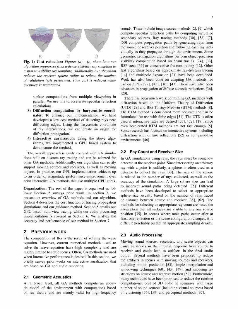
Fig. 1: Cost reduction: Figures (a) - (c) show how ouralgorithm progresses from a dense visibility ray sampling toa sparse visibility ray sampling. Additionally, our algorithmreduces the receiver sphere radius to reduce the numberof validation tests performed. Time cost is reduced whileaccuracy is maintained.

surface computations from multiple viewpoints inparallel. We use this to accelerate specular reflectioncalculations.

3) Diffraction computation by barycentric coordi-nates: To enhance our implementation, we havedeveloped a low cost method of detecting rays neardiffracting edges. Using the barycentric coordinateof ray intersections, we can create an origin fordiffraction propagation.

4) Interactive auralization: Using the above algo-rithms, we implemented a GPU based system todemonstrate the method.

The overall approach is easily coupled with GA simula-tions built on discrete ray tracing and can be adapted forother GA methods. Additionally, our algorithm can easilysupport moving sources and receivers, as well as movingobjects. In practice, our GPU implementation achieves upto an order of magnitude performance improvement overprior interactive GA methods that use multiple CPU cores.

Organization: The rest of the paper is organized as fol-lows: Section 2 surveys prior work. In section 3, wepresent an overview of GA methods and our algorithm.Section 4 describes the cost function of tracing propagationsimulations and our guidance method. Section 5 details ourGPU based multi-view tracing, while our audio processingimplementation is covered in Section 6. We analyze theaccuracy and performance of our method in Section 7.

2 PREVIOUS WORK

The computation of IRs is the result of solving the waveequation. However, current numerical methods used tosolve the wave equation have high complexity and aremainly limited to static scenes. Often, GA methods are usedwhen interactive performance is desired. In this section, webriefly survey prior works on interactive auralization thatare based on GA and audio rendering.

2.1 Geometric AcousticsAt a broad level, all GA methods compute an acous-tic model of the environment with computations basedon ray theory and are mainly valid for high-frequency

sounds. These include image source methods [2], [9] whichcompute specular reflection paths by computing virtual orsecondary sources. Ray tracing methods [30], [58], [7],[50] compute propagation paths by generating rays fromthe source or receiver position and following each ray indi-vidually as they propagate through the environment. Somegeometric propagation algorithms perform object-precisionvisibility computation based on beam tracing [24], [33],BSP trees [36] or conservative frustum tracing [12]. Otherfast algorithms based on approximate ray-frustum tracing[14] and multipole expansion [21] have been developed.Work has also been done on adapting GA methods foruse on GPUs [27], [43], [16], [47]. There have also beenadvances in propagation of diffuse acoustic reflections [36],[20].

There has been much work combining GA methods withdiffraction based on the Uniform Theory of Diffraction(UTD) [29] and Biot-Tolstoy-Medwin (BTM) methods [8].The BTM method is considered more accurate and can beformulated for use with finite edges [51]. The UTD is oftenused if interactive rates are desired [55], [52], [17], sinceeven accelerated BTM methods are not fast enough [5].Some research has focused on interactive systems includingdiffraction with diffuse reflections [52] or for game-likeenvironments [46].

2.2 Ray Count and Receiver Size

In GA simulations using rays, the rays must be somehowdetected at the receiver point. Since intersecting an arbitraryray with a point is unlikely, a sphere is often used as adetector to collect the rays [38]. The size of the sphereis related to the number of rays collected, as well as theaccuracy of the simulation. A large sphere size can leadto incorrect sound paths being detected [35]. Differentmethods have been developed to select an appropriatesphere size, usually based on the number of rays tracedor distance between source and receiver [35], [62]. Themethods for selecting an appropriate ray count are based theassumption that all surfaces are visible to any one sourceposition [35]. In scenes where most paths occur after atleast one reflection or the scene configuration changes, it isdifficult to reliably predict an appropriate sampling density.

2.3 Audio Processing

Moving sound sources, receivers, and scene objects cancause variations in the impulse response from source toreceiver and could lead to artifacts in the final audiooutput. Several methods have been proposed to reducethe artifacts in scenes with moving sources and receivers,including motion prediction [53], simple interpolation andwindowing techniques [60], [45], [49], and imposing re-strictions on source and receiver motion [52]. Furthermore,many techniques have been proposed to reduce the runtimecomputational cost of 3D audio in scenarios with largenumber of sound sources (including virtual sources) basedon clustering [56], [59] and perceptual methods [37].

3

R

SA

SB SB,C

S

B

C

A

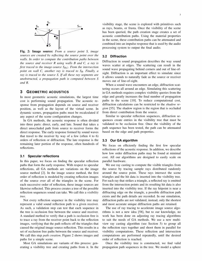
Fig. 2: Image source: From a source point S, imagesources are created by reflecting the source point over thewalls. In order to compute the contribution paths betweenthe source and receiver R using walls B and C, a ray isfirst traced to the image-source SB,C. From the intersectionpoint on wall C, another ray is traced to SB. Finally, aray is traced to the source S. If all these ray segments areunobstructed, a propagation path is computed between Sand R.

3 GEOMETRIC ACOUSTICSIn most geometric acoustic simulations, the largest timecost is performing sound propagation. The acoustic re-sponse from propagation depends on source and receiverposition, as well as the layout of the virtual scene. Indynamic scenes, propagation paths must be recalculated ifany aspect of the scene configuration changes.

In GA methods, the acoustic response is often dividedinto three parts: direct, early, and late. Sound that takes adirect unoccluded path from source to receiver forms thedirect response. The early response formed by sound wavesthat travel to the receiver by way of a few (often 4 to 6)orders of reflection or diffraction. The late response is theremaining later portion of the response, often hundreds ofreflections.

3.1 Specular reflectionsIn this paper, we focus on finding the specular reflectionpaths that form the early response. With respect to specularreflections, all GA methods are variations on the imagesource method [2]. In the image source method, the firstorder of reflection is modeled by creating reflection imagesof the source over all of the triangles in the scene. Foreach successive order of reflection, these image sources arelikewise reflected. This process creates a tree of the possiblereflection sequences sound can take. We call this a visibilitytree.

Not every reflection sequence in the visibility tree mayrepresent a valid sound reflection path to a given receiver.As such, a validation step can test that each sequence inthe tree is occlusion free between the source and receiver.A standard method to verify that a path is occlusion free isto trace a ray from the receiver point back to the reflectionimages, verifying that the path reflects off the triangles thatcaused the original image source reflection. This results in aset of occlusion free paths between the source and receiver.We call this step path creation. Figure 2 shows images andpaths for a simple scene.

Most GA simulations are variants of this process: gen-erating a visibility tree and creating paths from it. In the

visibility stage, the scene is explored with primitives suchas rays, beams, or frusta. Once the visibility of the scenehas been queried, the path creation stage creates a set ofacoustic contribution paths. Using the material propertiesin the scene, these contribution paths can be attenuated andcombined into an impulse response that is used by the audioprocessing system to output the final audio.

3.2 DiffractionDiffraction in sound propagation describes the way soundwaves scatter at edges. The scattering can result in thesound wave propagating behind corners and out of line-of-sight. Diffraction is an important effect to simulate sinceit allows sounds to naturally fade as the source or receivermoves out of line-of-sight.

When a sound wave encounters an edge, diffraction scat-tering occurs all around an edge. Simulating this scatteringin GA methods requires complex visibility queries from theedge and greatly increases the final number of propagationpaths in the scene [10]. To reduce computational cost,diffraction calculations can be restricted to the shadow re-gion [55]. The shadow region is the region that is occludedfrom direct contribution from the source.

Similar to specular reflection sequences, diffraction se-quences create entries in the visibility tree that must bevalidated to be occlusion free. Once the visibility of thepath sequence has been tested, the path can be attenuatedbased on the edge and path properties.

3.3 Our GA algorithmWe focus on efficiently finding the first few specularreflections of the acoustic response. In addition, we describehow low order diffraction paths may be found at minimalcost. All our algorithms are designed to easily scale onparallel hardware.

We use ray casting to compute the visible triangles fromthe source by tracing sample rays distributed randomlyaround the source point. These rays intersect the scenetriangles and the hit data is inserted into the visibility tree.For each ray that strikes a triangle, a reflected ray is emittedfrom the intersection points and its resulting hit data is alsoinserted into the visibility tree. If the ray hitpoint is near adiffracting edge on the triangle, a possible diffraction pathexists and the path details are recorded. In our simulation,diffraction paths are not validated, instead, only the shortestand most accurate unique diffraction paths are retained.

The use of ray tracing to accelerate image source algo-rithms is not a new idea [58], but to our knowledge, nowork has been done on adjusting ray tracing algorithmsto suit the needs of GA methods. We use a new multi-view ray casting algorithm (see Section 5) to group allthe reflection rays together and shoot them in parallel forvisibility computations. These reflection and intersectioncomputations are performed repeatedly, until the desiredorder of reflection is reached.

Once the visibility tree is constructed, we find validpropagation path sequences in the tree. We model a sphere

4

at the receiver and only visibility rays that intersect thesphere are validated. The accuracy of this approach isgoverned by the sampling density used in the primaryvisibility step and the size of the receiver sphere.

In addition to our new ray tracing algorithm, we proposea method to dynamically select appropriate sample densitiesand receiver sphere size during the simulation process.Section 4 details our approach to minimizing cost whilemaximizing accuracy.

4 GUIDED PROPAGATION

In this section we describe a cost function for specular GApropagation. We then describe our approach to reducing thenumber of tests conducted during propagation.

Some GA methods, such as beam tracing, compute a veryaccurate, minimal visibility tree. Since the reflection data inthe tree is very detailed, the complete set of valid paths canbe created very quickly [24]. However, generating such anaccurate tree is costly. Other methods, such as conservativefrustum culling [13], compute accurate trees that may beoverly conservative. The visibility tree can be generatedfaster, but the path creation time may increase, since someof the paths will be occluded and must be discarded. Thisconcept is similar for other GA based methods, leading toa simple cost function for specular propagation:

T =n

Âi=0

Si +n

Âi=0

m

Âj=0

Ri, j

Where T is the total cost of specular propagation, Si is thecost of generating the visibility tree for source i, and Ri, j iscost of path creation for source i to receiver j. Each sourcerequires separate visibility tree and path calculations. Itshould be noted that propagation paths are reciprocal whenignoring source and receiver directivity, so the endpointtypes can be swapped if it minimizes propagation cost.

4.1 Ray traced propagation cost

Sample based visibility methods like ray tracing are notguaranteed to generate an accurate visibility tree. This isbecause some triangles that are visible to the source maybe missed by the samples and incorrectly excluded fromthe visibility tree. However, ray tracing is still used insound propagation because of its high performance andease of implementation. Since our system uses ray basedpropagation, we focus our discussion on the cost of raytraced propagation.

The general form of ray traced propagation is to tracea distribution of visibility rays from the source into thescene, reflecting the rays to the desired order of recursion.A sphere of some radius is set at each receiver location andsome of the visibility rays may hit this detector sphere.The visibility rays that strike the sphere represent likelypropagation paths and should be validated to be occlusionfree.

(a)

(b)

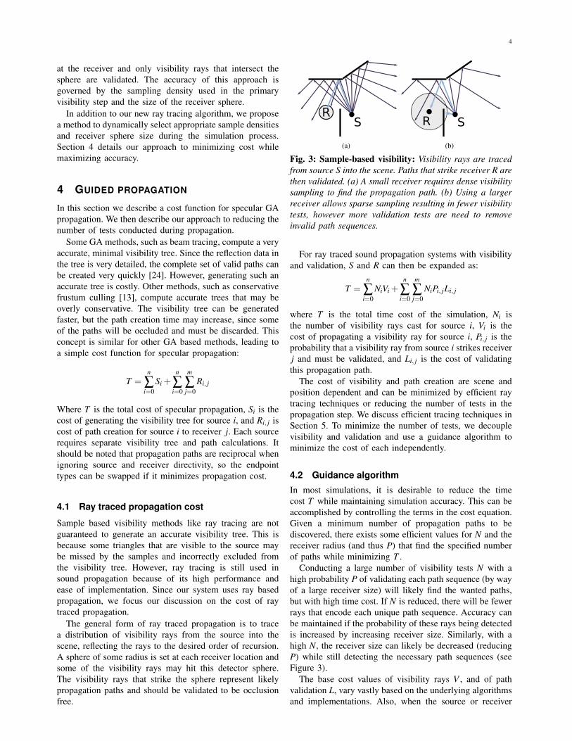
Fig. 3: Sample-based visibility: Visibility rays are tracedfrom source S into the scene. Paths that strike receiver R arethen validated. (a) A small receiver requires dense visibilitysampling to find the propagation path. (b) Using a largerreceiver allows sparse sampling resulting in fewer visibilitytests, however more validation tests are need to removeinvalid path sequences.

For ray traced sound propagation systems with visibilityand validation, S and R can then be expanded as:

T =n

Âi=0

NiVi +n

Âi=0

m

Âj=0

NiPi, jLi, j

where T is the total time cost of the simulation, Ni isthe number of visibility rays cast for source i, Vi is thecost of propagating a visibility ray for source i, Pi, j is theprobability that a visibility ray from source i strikes receiverj and must be validated, and Li, j is the cost of validatingthis propagation path.

The cost of visibility and path creation are scene andposition dependent and can be minimized by efficient raytracing techniques or reducing the number of tests in thepropagation step. We discuss efficient tracing techniques inSection 5. To minimize the number of tests, we decouplevisibility and validation and use a guidance algorithm tominimize the cost of each independently.

4.2 Guidance algorithmIn most simulations, it is desirable to reduce the timecost T while maintaining simulation accuracy. This can beaccomplished by controlling the terms in the cost equation.Given a minimum number of propagation paths to bediscovered, there exists some efficient values for N and thereceiver radius (and thus P) that find the specified numberof paths while minimizing T .

Conducting a large number of visibility tests N with ahigh probability P of validating each path sequence (by wayof a large receiver size) will likely find the wanted paths,but with high time cost. If N is reduced, there will be fewerrays that encode each unique path sequence. Accuracy canbe maintained if the probability of these rays being detectedis increased by increasing receiver size. Similarly, with ahigh N, the receiver size can likely be decreased (reducingP) while still detecting the necessary path sequences (seeFigure 3).

The base cost values of visibility rays V , and of pathvalidation L, vary vastly based on the underlying algorithmsand implementations. Also, when the source or receiver

5

Fig. 4: Propagation test count: With a goal of finding90% of the total paths in the scene, an increasing numberof visibility rays are traced and the minimum required sizeof the receiver sphere changes accordingly. With sparsevisibility sampling, a large sphere is required, resulting inmany validation tests. With dense sampling, the sphere sizecan be reduced. For specific cost values for visibility andpath validation tests, some minimal total cost exists.

move, or objects in the scene move, V and L can change,altering the total cost function. Indeed, since the optimalvalues may change throughout the course of the simulation,it is difficult to find the best values to reduce the time cost.

Instead of attempting to find the optimal values, ourguidance algorithm seeks to independently minimize thenumber of visibility and validation tests used in propaga-tion. It works by adjusting the number of visibility rayscast and the size of the detection sphere. These two factorscorrespond to N and P, respectively. Figure 4 shows anexample cost function in terms of the minimal number oftests needed to find a specific percentage of the total pathsin a scene.

Our algorithm monitors the count of unique contributionpaths found during a single simulation frame. The goal onsubsequent frames is to find an equal or greater number ofpaths to this maximum recorded path count, while usinga minimal number of visibility and validation tests. Thealgorithm achieves this by reducing the number of raystraced and the size of the detection sphere. If at any timethe path count decreases (i.e. a path is lost), the algorithmresponds by increasing the number of rays and receiver sizeuntil the path is recovered. If the path cannot be recoveredafter aggressive adjustment, the lower path count is selectedas the maximum known path count. If at any time thecurrent path count exceeds the recorded maximum count,the maximum count is updated to the new higher count.This allows our method to respond conservatively to scenechanges.

On startup, the algorithm begins by tracing a user spec-ified number of rays and with a user specified receiversphere size. We use 50k rays and a sphere radius of 1

4

Fig. 5: Guiding state machine: This state machine tracksthe number of unique contribution paths found. Solid linesare followed if the current path count matches the recordedmaximum count, dashed lines are followed if the path countis less than the recorded maximum. States marked R+ andS+ increase the ray count and sphere size, while statesmarked R� and S� decrease the ray count and sphere size,respectively. At the Restart state, the maximum paths countis set to the current count. The (R+,S+) states attempt torecover lost paths before recording a new count. The maintop and bottom arms focus on reducing rays and receiversize respectively.

the length of the maximal scene axis in our tests. From thispoint, the number of rays and sphere size are reduced to findlocal minima of the total cost function without decreasingaccuracy. A small initial number of visibility rays can leadto sampling errors that are further discussed in Section 7.

Our guiding algorithm is easily represented as a statemachine. Figure 5 shows the details of the state machine.After each simulation cycle a new state is found and thepropagation parameters are adjusted. This process contin-uously adjusts the number of rays traced and the sizeof the receiver spheres. Each receiver sphere is adjustedindependently; if the state machine enters a state wheresphere size is increased, but no paths have been missedto a certain receiver, that specific receiver sphere is notincreased. The accuracy and performance of the algorithmis discussed in Section 7.

5 MULTI-VIEW GPU RAY TRACING

We use a high performance GPU ray tracer to conductthe visibility and validation tests needed during soundpropagation. To further improve performance, we attemptto process each specular view in parallel independentlyusing a multi-view tracing approach. We describe our basicGPU ray tracer, the multi-view tracing process, and ourdiffraction and validation approaches.

5.1 GPU Propagation

We divide the processing work between the host and GPUdevice. The host handles all audio processing, while theGPU device computes the propagation results. Figure 6shows the overall details. Our propagation algorithm tracesvisibility rays through the scene, intersects them with areceiver sphere, and validates the possible propagationpaths to be occlusion free.

6

Fig. 6: Implementation Overview: All scene processing and propagation takes place on the GPU: hierarchy construction,visibility computations, specular and edge diffraction. The sound paths computed using GPU processing are returned tothe host for guidance analysis and audio processing. The guidance results are used to direct the next propagation cycle.

For general ray tracing, previous approaches have in-vestigated efficient methods to implement ray tracing onmassively parallel architectures such as GPUs, which havea high number of cores as well as wide vector units on eachcore. Current methods for GPU-based ray tracing mainlydiffer in the choice of acceleration structure such as kd-trees [64] or BVHs and the parallelization of ray traversalstep on each GPU core. For example, rays can be traced asa packet similar to CPU SIMD ray tracing [42] and somerecent approaches can evaluate them independently [1], asmore memory is available for local computation on currentGPUs.

We build on the bounding volume hierarchy (BVH) raytracing ideas in [34] and implement our multi-view raycasting system in CUDA. This allows us to render sceneswith dynamic geometry, as the BVH can be refit or rebuiltas needed. While NVIDIA provides a ray tracing system[39] for use on CUDA hardware, we use our own fast raytracer due to its flexibility.

Rays are bundled into packets that are executed oneach core while scheduling each ray on a lane in thevector unit. The rays are then traversed through the BVHand intersected against the triangles. For primary visibilitysamples, we use a simple ray tracing kernel that exploits thecommon ray sources for efficiency. Reflections are handledby a secondary kernel which loads the previous hit dataand traces a reflection ray. To decouple the number ofvisibility samples from the number of threads allocatedfor processing, we iteratively process visibility samples insmall thread blocks until all samples have been traced.As rays exit the scene, they are removed from the workqueue and no longer processed. The algorithm ends whenno more active samples exist or the maximum recursiondepth is reached in terms of reflections. At any point duringtracing, if the ray coherence is reduced past a user specifiedthreshold, multi-view tracing is employed.

Once the visibility computations have been performed upto a specified order of reflection, the visibility data is testedagainst the receiver spheres. Each ray is tested against eachreceiver sphere for intersection and is marked if it hits thesphere and needs to be included in the path validation tests.

As a final step, once the receiver intersect tests arecomplete, we compute the valid contribution paths to thereceiver. For each valid path, image source and triangle datais retrieved. A test checks if the line connecting the sourceimage point to the receiver passes through the associated

triangle. This test immediately discards most invalid paths.Then, for each receiver, a ray is constructed from thereceiver towards each image point and traced through thescene. From the resulting hit point, a new ray is traced tothe parent image, continuing back to the initial source point.If the entire path is unoccluded, there is a contribution.

5.2 Multi-View TracingThe underlying formulation of the image source method issuch that each reflection path can be evaluated indepen-dently. When using ray tracing visibility with the imagesource method, all visibility and validation tests are alsoindependent. As such it is possible to evaluate queries inparallel. For example, if there are multiple sound imagesources, we may perform visibility computations from eachof them in parallel. Our multi-view algorithm exploitsthis: in order to achieve high performance, we process allindependent visibility and validation tests simultaneously.

When considering specular reflection rays, it is helpfulto view rays as visibility queries that accelerate the imagesource process. From the source point, the ray visibilityquery returns the set of triangles visible to the source (sub-ject to sampling error). From this set of visible triangles,image sources can be created by reflecting the source pointover each triangle face. New samples can then be generatedon each triangle face, forming a reflection visibility querywith the image point at the ray origin. This process repeatsto the recursion limit.

In our case, it is natural to bundle all the reflected visibil-ity samples from one origin together in ray packets. Sincethe main factor determining performance in our packetbased ray tracer is ray coherence, such bundling allowsefficient use of memory bandwidth and SIMD vector units.As described in the previous section, primary visibility raysare easy to group into coherent packets. However, as therays are reflected, it is likely that the rays in the packetwill hit different triangles, and thus be reflected in differentdirections with different ray origins. As a result, the packetsare less coherent and may require multiple queries to theBVH, thus wasting computational resources.

On the GPU, each thread block is treated as if it isrunning on independent hardware from all other blocks.Our ray packets are formed with a ray for each thread inthe thread block. When all the rays in a packet share acommon origin, the packet represents a single ray tracedview that can be traced very efficiently. The goal of our

7

(a) (b) (c)

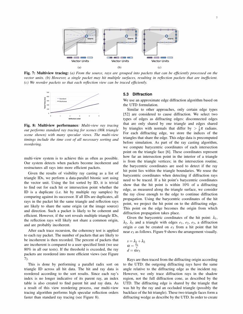
Fig. 7: Multiview tracing: (a) From the source, rays are grouped into packets that can be efficiently processed on thevector units. (b) However, a single packet may hit multiple surfaces, resulting in reflection packets that are inefficient.(c) We reorder packets so that each reflection view can be traced efficiently.

Fig. 8: Multiview performance: Multi-view ray tracingout performs standard ray tracing for scenes (80k trianglescene shown) with many specular views. The multi-viewtimings include the time cost of all necessary sorting andreordering.

multi-view system is to achieve this as often as possible.Our system detects when packets become incoherent andrestructures all rays into more efficient packets.

Given the results of visibility ray casting as a list oftriangle IDs, we perform a data-parallel bitonic sort usingthe vector unit. Using the list sorted by ID, it is trivialto find out for each hit or intersection point whether theID is a duplicate (i.e. hit by multiple ray samples) bycomparing against its successor. If all IDs are duplicates, allrays in the packet hit the same triangle and reflection raysare likely to share the same origin (at the image source)and direction. Such a packet is likely to be coherent andefficient. However, if the sort reveals multiple triangle IDs,the reflection rays will likely not share a common origin,and are probably incoherent.

After each trace recursion, the coherency test is appliedto each ray packet. The number of packets that are likely tobe incoherent is then recorded. The percent of packets thatare incoherent is compared to a user specified limit (we use80% in all our tests). If the threshold is exceeded, the raypackets are reordered into more efficient views (see Figure7).

This is done by performing a parallel radix sort ontriangle ID across all hit data. The hit and ray data isreordered according to the sort results. Since each ray’sindex is no longer indicative of its parent ray, an indextable is also created to find parent hit and ray data. Asa result of this view reordering process, our multi-viewtracing algorithm performs high specular reflection ordersfaster than standard ray tracing (see Figure 8).

5.3 DiffractionWe use an approximate edge diffraction algorithm based onthe UTD formulation.

Similar to other approaches, only certain edge types[52] are considered to cause diffraction. We select twotypes of edges as diffracting edges: disconnected edgesthat are only shared by one triangle and edges sharedby triangles with normals that differ by > 1

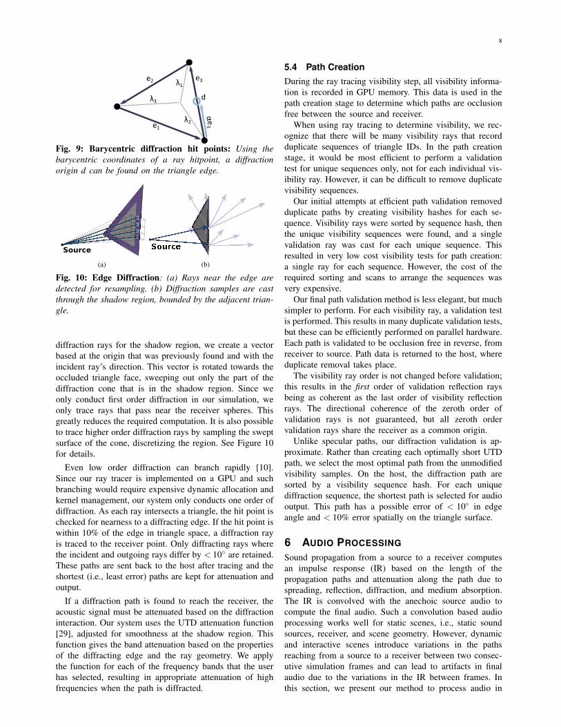
8 p radians.For each diffracting edge, we store the indices of thetriangles that share the edge. This edge data is precomputedbefore simulation. As part of the ray casting algorithm,we compute barycentric coordinates of each intersectionpoint on the triangle face [6]. These coordinates representhow far an intersection point in the interior of a triangleis from the triangle vertices; in the intersection routine,the barycentric coordinates are used to detect if the rayhit point lies within the triangle boundaries. We reuse thebarycentric coordinates when detecting if diffraction raysneed to be traced. If a hit point’s barycentric coordinatesshow that the hit point is within 10% of a diffractingedge, as measured along the triangle surface, we considerthe ray close enough to the edge to continue diffractionpropagation. Using the barycentric coordinates of the hitpoint, we project the hit point on to the diffracting edge.This point on the edge becomes the origin from whichdiffraction propagation takes place.

Given the barycentric coordinates of the hit point: l1,l2, l3 and a triangle with edges e1, e2, e3, a diffractionorigin o can be created on e3 from a hit point that hitnear e3 as follows. Figure 9 shows the arrangement visually.

s = l1 +l2a = l2

sd = ae3

Rays are then traced from the diffracting origin accordingto the UTD: the outgoing diffracting rays have the sameangle relative to the diffracting edge as the incident ray.However, we only trace diffraction rays in the shadowregion, not the full diffraction cone, as described by theUTD. The diffracting edge is shared by the triangle thatwas hit by the ray and an occluded triangle (possibly thebackface of the hit triangle). These two triangle faces form adiffracting wedge as describe by the UTD. In order to create

8

Fig. 9: Barycentric diffraction hit points: Using thebarycentric coordinates of a ray hitpoint, a diffractionorigin d can be found on the triangle edge.

Source

(a)

Source

(b)

Fig. 10: Edge Diffraction: (a) Rays near the edge aredetected for resampling. (b) Diffraction samples are castthrough the shadow region, bounded by the adjacent trian-gle.

diffraction rays for the shadow region, we create a vectorbased at the origin that was previously found and with theincident ray’s direction. This vector is rotated towards theoccluded triangle face, sweeping out only the part of thediffraction cone that is in the shadow region. Since weonly conduct first order diffraction in our simulation, weonly trace rays that pass near the receiver spheres. Thisgreatly reduces the required computation. It is also possibleto trace higher order diffraction rays by sampling the sweptsurface of the cone, discretizing the region. See Figure 10for details.

Even low order diffraction can branch rapidly [10].Since our ray tracer is implemented on a GPU and suchbranching would require expensive dynamic allocation andkernel management, our system only conducts one order ofdiffraction. As each ray intersects a triangle, the hit point ischecked for nearness to a diffracting edge. If the hit point iswithin 10% of the edge in triangle space, a diffraction rayis traced to the receiver point. Only diffracting rays wherethe incident and outgoing rays differ by < 10� are retained.These paths are sent back to the host after tracing and theshortest (i.e., least error) paths are kept for attenuation andoutput.

If a diffraction path is found to reach the receiver, theacoustic signal must be attenuated based on the diffractioninteraction. Our system uses the UTD attenuation function[29], adjusted for smoothness at the shadow region. Thisfunction gives the band attenuation based on the propertiesof the diffracting edge and the ray geometry. We applythe function for each of the frequency bands that the userhas selected, resulting in appropriate attenuation of highfrequencies when the path is diffracted.

5.4 Path CreationDuring the ray tracing visibility step, all visibility informa-tion is recorded in GPU memory. This data is used in thepath creation stage to determine which paths are occlusionfree between the source and receiver.

When using ray tracing to determine visibility, we rec-ognize that there will be many visibility rays that recordduplicate sequences of triangle IDs. In the path creationstage, it would be most efficient to perform a validationtest for unique sequences only, not for each individual vis-ibility ray. However, it can be difficult to remove duplicatevisibility sequences.

Our initial attempts at efficient path validation removedduplicate paths by creating visibility hashes for each se-quence. Visibility rays were sorted by sequence hash, thenthe unique visibility sequences were found, and a singlevalidation ray was cast for each unique sequence. Thisresulted in very low cost visibility tests for path creation:a single ray for each sequence. However, the cost of therequired sorting and scans to arrange the sequences wasvery expensive.

Our final path validation method is less elegant, but muchsimpler to perform. For each visibility ray, a validation testis performed. This results in many duplicate validation tests,but these can be efficiently performed on parallel hardware.Each path is validated to be occlusion free in reverse, fromreceiver to source. Path data is returned to the host, whereduplicate removal takes place.

The visibility ray order is not changed before validation;this results in the first order of validation reflection raysbeing as coherent as the last order of visibility reflectionrays. The directional coherence of the zeroth order ofvalidation rays is not guaranteed, but all zeroth ordervalidation rays share the receiver as a common origin.

Unlike specular paths, our diffraction validation is ap-proximate. Rather than creating each optimally short UTDpath, we select the most optimal path from the unmodifiedvisibility samples. On the host, the diffraction path aresorted by a visibility sequence hash. For each uniquediffraction sequence, the shortest path is selected for audiooutput. This path has a possible error of < 10� in edgeangle and < 10% error spatially on the triangle surface.

6 AUDIO PROCESSINGSound propagation from a source to a receiver computesan impulse response (IR) based on the length of thepropagation paths and attenuation along the path due tospreading, reflection, diffraction, and medium absorption.The IR is convolved with the anechoic source audio tocompute the final audio. Such a convolution based audioprocessing works well for static scenes, i.e., static soundsources, receiver, and scene geometry. However, dynamicand interactive scenes introduce variations in the pathsreaching from a source to a receiver between two consec-utive simulation frames and can lead to artifacts in finalaudio due to the variations in the IR between frames. Inthis section, we present our method to process audio in

9

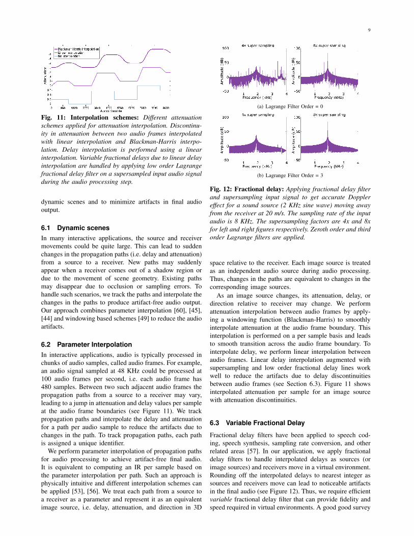
Fig. 11: Interpolation schemes: Different attenuationschemes applied for attenuation interpolation. Discontinu-ity in attenuation between two audio frames interpolatedwith linear interpolation and Blackman-Harris interpo-lation. Delay interpolation is performed using a linearinterpolation. Variable fractional delays due to linear delayinterpolation are handled by applying low order Lagrangefractional delay filter on a supersampled input audio signalduring the audio processing step.

dynamic scenes and to minimize artifacts in final audiooutput.

6.1 Dynamic scenesIn many interactive applications, the source and receivermovements could be quite large. This can lead to suddenchanges in the propagation paths (i.e. delay and attenuation)from a source to a receiver. New paths may suddenlyappear when a receiver comes out of a shadow region ordue to the movement of scene geometry. Existing pathsmay disappear due to occlusion or sampling errors. Tohandle such scenarios, we track the paths and interpolate thechanges in the paths to produce artifact-free audio output.Our approach combines parameter interpolation [60], [45],[44] and windowing based schemes [49] to reduce the audioartifacts.

6.2 Parameter InterpolationIn interactive applications, audio is typically processed inchunks of audio samples, called audio frames. For example,an audio signal sampled at 48 KHz could be processed at100 audio frames per second, i.e. each audio frame has480 samples. Between two such adjacent audio frames thepropagation paths from a source to a receiver may vary,leading to a jump in attenuation and delay values per sampleat the audio frame boundaries (see Figure 11). We trackpropagation paths and interpolate the delay and attenuationfor a path per audio sample to reduce the artifacts due tochanges in the path. To track propagation paths, each pathis assigned a unique identifier.

We perform parameter interpolation of propagation pathsfor audio processing to achieve artifact-free final audio.It is equivalent to computing an IR per sample based onthe parameter interpolation per path. Such an approach isphysically intuitive and different interpolation schemes canbe applied [53], [56]. We treat each path from a source toa receiver as a parameter and represent it as an equivalentimage source, i.e. delay, attenuation, and direction in 3D

(a) Lagrange Filter Order = 0

(b) Lagrange Filter Order = 3

Fig. 12: Fractional delay: Applying fractional delay filterand supersampling input signal to get accurate Dopplereffect for a sound source (2 KHz sine wave) moving awayfrom the receiver at 20 m/s. The sampling rate of the inputaudio is 8 KHz. The supersampling factors are 4x and 8xfor left and right figures respectively. Zeroth order and thirdorder Lagrange filters are applied.

space relative to the receiver. Each image source is treatedas an independent audio source during audio processing.Thus, changes in the paths are equivalent to changes in thecorresponding image sources.

As an image source changes, its attenuation, delay, ordirection relative to receiver may change. We performattenuation interpolation between audio frames by apply-ing a windowing function (Blackman-Harris) to smoothlyinterpolate attenuation at the audio frame boundary. Thisinterpolation is performed on a per sample basis and leadsto smooth transition across the audio frame boundary. Tointerpolate delay, we perform linear interpolation betweenaudio frames. Linear delay interpolation augmented withsupersampling and low order fractional delay lines workwell to reduce the artifacts due to delay discontinuitiesbetween audio frames (see Section 6.3). Figure 11 showsinterpolated attenuation per sample for an image sourcewith attenuation discontinuities.

6.3 Variable Fractional Delay

Fractional delay filters have been applied to speech cod-ing, speech synthesis, sampling rate conversion, and otherrelated areas [57]. In our application, we apply fractionaldelay filters to handle interpolated delays as sources (orimage sources) and receivers move in a virtual environment.Rounding off the interpolated delays to nearest integer assources and receivers move can lead to noticeable artifactsin the final audio (see Figure 12). Thus, we require efficientvariable fractional delay filter that can provide fidelity andspeed required in virtual environments. A good good survey

10

of FIR and IIR filter design for fractional delay filter isprovided in [32].

We use a Lagrange interpolation filter due to explicitformulas to a construct fractional delay filter and flat-frequency response for low-frequencies. Combined withsupersampled input audio signal, we can model fractionaldelay accurately. Variable delay can be easily modeled byusing a different filter computed explicitly per audio sam-ple. To compute an order N Lagrange filter, the traditionalmethods [57] require Q(N2) time and Q(1) space. However,the same computation can be reduced to Q(N) time andQ(N) space complexity [23]. Many applications requiringvariable fractional delay oversample the input with a high-order interpolator and use a low-order variable fractionaldelay interpolator [61] to avoid computing a high-ordervariable delay filter during run time. Wise and Bristow-Johnson [61] analyze the signal-to-noise-ratio (SNR) forvarious low-order polynomial interpolators in the presenceof oversampled input. Thus, for a given SNR requirement,optimal supersampled input signal and low-order polyno-mial interpolator can be chosen to minimize computationaland space complexity. Ideally, a highly oversampled inputsignal is required (see Figure 12) to achieve 60 dB or moreSNR for a low-order Lagrange interpolation filter, but itmight be possible to use low oversampling to minimizeartifacts in final audio output [45].

7 ANALYSIS

In this section, we analyze the performance of our algo-rithm, highlight the error sources, and compare it with priormethods.

7.1 PerformanceWe have used our algorithms on several different scenariosand scenes. The complexity of these scenes is similar tothose used in current games with tens of thousands oftriangles for audio processing. We test the performance ofthe system on a multi-core PC with NVIDIA GTX 480GPU and use a single CPU core (2.8 GHz Pentium) foraudio processing. We used some common benchmarks toevaluate the performance of our system (Figure 13). Resultsfor static source and receiver positions are shown in Table 1.We also show the cost of conducting higher order recursionin Table 2.

In addition to static scenes, we show results with dy-namic movement in the Music hall scene using a 500 framesequence. For this test, we use the coordinates defined inthe round robin III dataset 1. The source and receiver beginat coordinates S1 and R1, respectively. Over frames 100-200, the source moves linearly from S1 to S2. Over frames300-400, the receiver moves linearly from R1 to R2. Wecompare our guidance method to other receiver size models.In each method, r is the predicted receiver radius, N is theray count, V is the scene volume, ` is the ray length, andd is the distance between source and receiver.

1. http://www.ptb.de/en/org/1/16/163/roundrobin/roundrobin.htm

• Lehnert model: This model increases the receiverradius for rays that travel farther, adjusting the radiusas rays spread out [35].r = `

q2pN

• NORMAL model: Originally a method for predictingthe number of rays needed based on scene volume[19], [63], this algorithm has been adapted as a receiversize model [62].r = 3

q15V2pN

• Xiangyang model: This model accounts for the min-imal sphere receiver size needed for detection andadjusts the radius based on scene volume [62].r = log10(V )d

q4N

It should be noted that these receiver models are intendedfor simulations that include high orders of diffuse reflec-tions and are not necessarily optimal for low orders of spec-ular reflections. Each of these receiver models have beenimplemented in a parallel efficient manner and integratedinto our simulation. All simulations begin with 50,000rays. Appendix A shows detailed data for the animationsequence.

Model #Tri Bounces #Paths PT (ms) AT (ms)Desert 35k 3R+1D 15 53 3

Indoor scene 1.5k 3R+1D 27 62 5Music Hall 0.2k 3R 62 23 7

Sibenik 80k 2R 11 90 3TABLE 1: Performance in static scenes: The top tworepresent simple indoor and outdoor scenes. The third oneis a well known acoustic benchmark and the fourth one isthe model of Sibenik Cathedral. The number of reflections(R) and edge diffraction (D) are given in the second column.The time spent in computing propagation paths (on GPU)is shown in the PT column and audio processing (on CPU)is shown in the AT column. The simulation begins with 50kvisibility samples; we measure the performance after 50frames.

Model 1R 2R 3R 4RDesert 30 41 53 57Sibenik 51 90 153 226

TABLE 2: Performance per recursion: Average perfor-mance (in ms) of our GPU-based path computation algo-rithm as a function of number of reflections performed. TheDesert scene also includes edge diffraction. 50k visibilitysamples were used.

7.2 Accuracy and LimitationsOverall, our approach is designed to exploit the compu-tational power of GPUs to perform interactive visibilityqueries. The overall goal is accurate auralization, but ourapproach can result in the following errors:

1. Visibility errors: The accuracy of the visible sur-face or secondary image source computation algorithmis governed by the number of ray samples and relativeconfiguration of the image sources. Our algorithm canmiss some secondary sources or propagation paths and is

11

(a) (b) (c) (d)

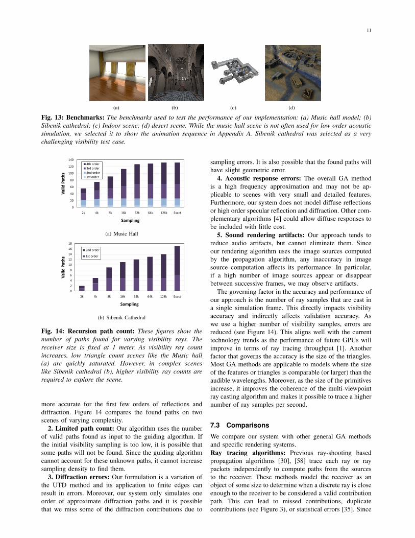
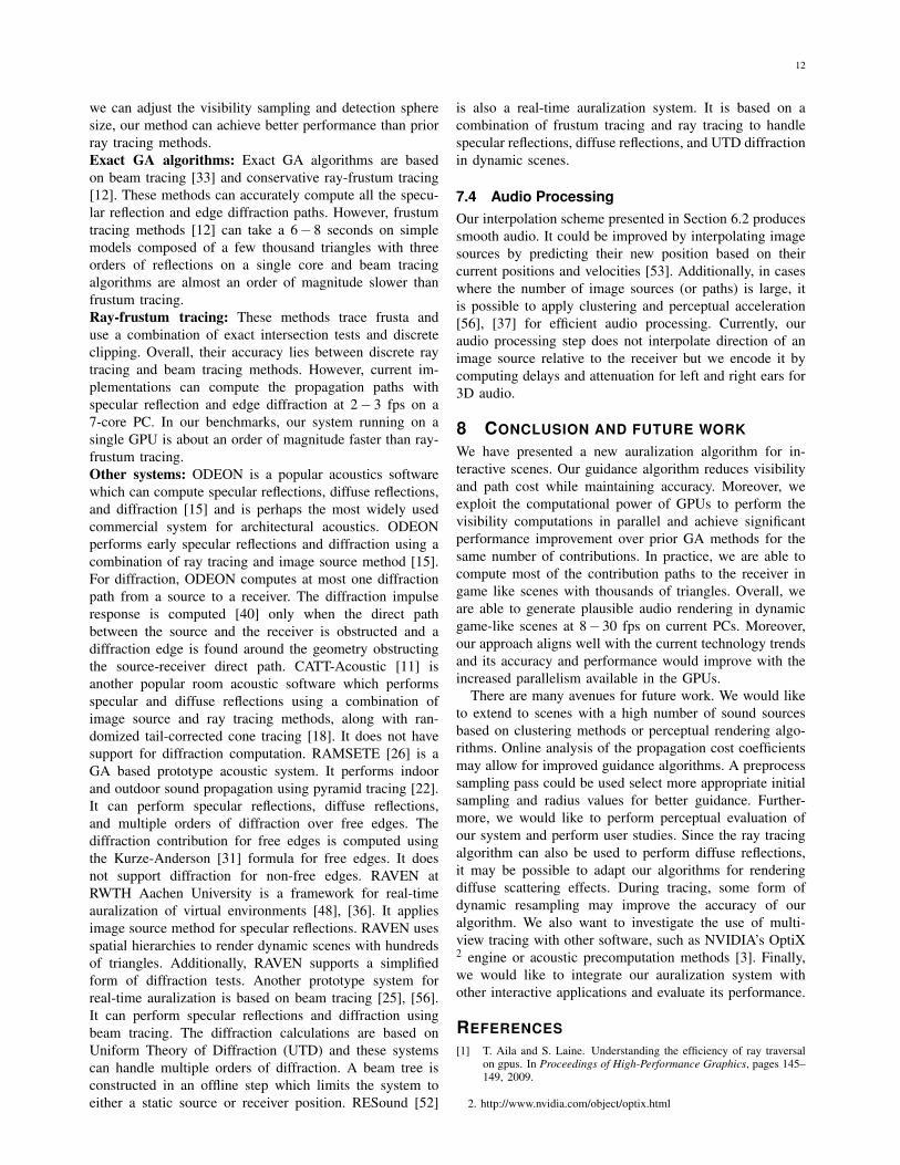
Fig. 13: Benchmarks: The benchmarks used to test the performance of our implementation: (a) Music hall model; (b)Sibenik cathedral; (c) Indoor scene; (d) desert scene. While the music hall scene is not often used for low order acousticsimulation, we selected it to show the animation sequence in Appendix A. Sibenik cathedral was selected as a verychallenging visibility test case.

(a) Music Hall

(b) Sibenik Cathedral

Fig. 14: Recursion path count: These figures show thenumber of paths found for varying visibility rays. Thereceiver size is fixed at 1 meter. As visibility ray countincreases, low triangle count scenes like the Music hall(a) are quickly saturated. However, in complex sceneslike Sibenik cathedral (b), higher visibility ray counts arerequired to explore the scene.

more accurate for the first few orders of reflections anddiffraction. Figure 14 compares the found paths on twoscenes of varying complexity.

2. Limited path count: Our algorithm uses the numberof valid paths found as input to the guiding algorithm. Ifthe initial visibility sampling is too low, it is possible thatsome paths will not be found. Since the guiding algorithmcannot account for these unknown paths, it cannot increasesampling density to find them.

3. Diffraction errors: Our formulation is a variation ofthe UTD method and its application to finite edges canresult in errors. Moreover, our system only simulates oneorder of approximate diffraction paths and it is possiblethat we miss some of the diffraction contributions due to

sampling errors. It is also possible that the found paths willhave slight geometric error.

4. Acoustic response errors: The overall GA methodis a high frequency approximation and may not be ap-plicable to scenes with very small and detailed features.Furthermore, our system does not model diffuse reflectionsor high order specular reflection and diffraction. Other com-plementary algorithms [4] could allow diffuse responses tobe included with little cost.

5. Sound rendering artifacts: Our approach tends toreduce audio artifacts, but cannot eliminate them. Sinceour rendering algorithm uses the image sources computedby the propagation algorithm, any inaccuracy in imagesource computation affects its performance. In particular,if a high number of image sources appear or disappearbetween successive frames, we may observe artifacts.

The governing factor in the accuracy and performance ofour approach is the number of ray samples that are cast ina single simulation frame. This directly impacts visibilityaccuracy and indirectly affects validation accuracy. Aswe use a higher number of visibility samples, errors arereduced (see Figure 14). This aligns well with the currenttechnology trends as the performance of future GPUs willimprove in terms of ray tracing throughput [1]. Anotherfactor that governs the accuracy is the size of the triangles.Most GA methods are applicable to models where the sizeof the features or triangles is comparable (or larger) than theaudible wavelengths. Moreover, as the size of the primitivesincrease, it improves the coherence of the multi-viewpointray casting algorithm and makes it possible to trace a highernumber of ray samples per second.

7.3 ComparisonsWe compare our system with other general GA methodsand specific rendering systems.Ray tracing algorithms: Previous ray-shooting basedpropagation algorithms [30], [58] trace each ray or raypackets independently to compute paths from the sourcesto the receiver. These methods model the receiver as anobject of some size to determine when a discrete ray is closeenough to the receiver to be considered a valid contributionpath. This can lead to missed contributions, duplicatecontributions (see Figure 3), or statistical errors [35]. Since

12

we can adjust the visibility sampling and detection spheresize, our method can achieve better performance than priorray tracing methods.Exact GA algorithms: Exact GA algorithms are basedon beam tracing [33] and conservative ray-frustum tracing[12]. These methods can accurately compute all the specu-lar reflection and edge diffraction paths. However, frustumtracing methods [12] can take a 6� 8 seconds on simplemodels composed of a few thousand triangles with threeorders of reflections on a single core and beam tracingalgorithms are almost an order of magnitude slower thanfrustum tracing.Ray-frustum tracing: These methods trace frusta anduse a combination of exact intersection tests and discreteclipping. Overall, their accuracy lies between discrete raytracing and beam tracing methods. However, current im-plementations can compute the propagation paths withspecular reflection and edge diffraction at 2� 3 fps on a7-core PC. In our benchmarks, our system running on asingle GPU is about an order of magnitude faster than ray-frustum tracing.Other systems: ODEON is a popular acoustics softwarewhich can compute specular reflections, diffuse reflections,and diffraction [15] and is perhaps the most widely usedcommercial system for architectural acoustics. ODEONperforms early specular reflections and diffraction using acombination of ray tracing and image source method [15].For diffraction, ODEON computes at most one diffractionpath from a source to a receiver. The diffraction impulseresponse is computed [40] only when the direct pathbetween the source and the receiver is obstructed and adiffraction edge is found around the geometry obstructingthe source-receiver direct path. CATT-Acoustic [11] isanother popular room acoustic software which performsspecular and diffuse reflections using a combination ofimage source and ray tracing methods, along with ran-domized tail-corrected cone tracing [18]. It does not havesupport for diffraction computation. RAMSETE [26] is aGA based prototype acoustic system. It performs indoorand outdoor sound propagation using pyramid tracing [22].It can perform specular reflections, diffuse reflections,and multiple orders of diffraction over free edges. Thediffraction contribution for free edges is computed usingthe Kurze-Anderson [31] formula for free edges. It doesnot support diffraction for non-free edges. RAVEN atRWTH Aachen University is a framework for real-timeauralization of virtual environments [48], [36]. It appliesimage source method for specular reflections. RAVEN usesspatial hierarchies to render dynamic scenes with hundredsof triangles. Additionally, RAVEN supports a simplifiedform of diffraction tests. Another prototype system forreal-time auralization is based on beam tracing [25], [56].It can perform specular reflections and diffraction usingbeam tracing. The diffraction calculations are based onUniform Theory of Diffraction (UTD) and these systemscan handle multiple orders of diffraction. A beam tree isconstructed in an offline step which limits the system toeither a static source or receiver position. RESound [52]

is also a real-time auralization system. It is based on acombination of frustum tracing and ray tracing to handlespecular reflections, diffuse reflections, and UTD diffractionin dynamic scenes.

7.4 Audio ProcessingOur interpolation scheme presented in Section 6.2 producessmooth audio. It could be improved by interpolating imagesources by predicting their new position based on theircurrent positions and velocities [53]. Additionally, in caseswhere the number of image sources (or paths) is large, itis possible to apply clustering and perceptual acceleration[56], [37] for efficient audio processing. Currently, ouraudio processing step does not interpolate direction of animage source relative to the receiver but we encode it bycomputing delays and attenuation for left and right ears for3D audio.

8 CONCLUSION AND FUTURE WORKWe have presented a new auralization algorithm for in-teractive scenes. Our guidance algorithm reduces visibilityand path cost while maintaining accuracy. Moreover, weexploit the computational power of GPUs to perform thevisibility computations in parallel and achieve significantperformance improvement over prior GA methods for thesame number of contributions. In practice, we are able tocompute most of the contribution paths to the receiver ingame like scenes with thousands of triangles. Overall, weare able to generate plausible audio rendering in dynamicgame-like scenes at 8� 30 fps on current PCs. Moreover,our approach aligns well with the current technology trendsand its accuracy and performance would improve with theincreased parallelism available in the GPUs.

There are many avenues for future work. We would liketo extend to scenes with a high number of sound sourcesbased on clustering methods or perceptual rendering algo-rithms. Online analysis of the propagation cost coefficientsmay allow for improved guidance algorithms. A preprocesssampling pass could be used select more appropriate initialsampling and radius values for better guidance. Further-more, we would like to perform perceptual evaluation ofour system and perform user studies. Since the ray tracingalgorithm can also be used to perform diffuse reflections,it may be possible to adapt our algorithms for renderingdiffuse scattering effects. During tracing, some form ofdynamic resampling may improve the accuracy of ouralgorithm. We also want to investigate the use of multi-view tracing with other software, such as NVIDIA’s OptiX2 engine or acoustic precomputation methods [3]. Finally,we would like to integrate our auralization system withother interactive applications and evaluate its performance.

REFERENCES[1] T. Aila and S. Laine. Understanding the efficiency of ray traversal

on gpus. In Proceedings of High-Performance Graphics, pages 145–149, 2009.

2. http://www.nvidia.com/object/optix.html

13

[2] J. B. Allen and D. A. Berkley. Image method for efficientlysimulating small-room acoustics. The Journal of the AcousticalSociety of America, 65(4):943–950, April 1979.

[3] L. Antani, A. Chandak, L. Savioja, and D. Manocha. In-teractive sound propagation using compact acoustic transferoperators. ACM Transactions on Graphics (To appear).http://www.cs.unc.edu/ lakulish/Papers/2011-tog.pdf.

[4] L. Antani, A. Chandak, M. Taylor, and D. Manocha. Direct-to-indirect acoustic radiance transfer. IEEE Transactions on Visualiza-tion and Computer Graphics, 18(2):261 – 269, February 2012.

[5] L. Antani, A. Chankak, M. Taylor, and D. Manocha. Fast geometricsound propagation with finite edge diffraction. Technical ReportTR10-011, University of North Carolina, Chapel Hill, 2010.

[6] J. Arenberg. Re: Ray/triangle intersection with barycentric coordi-nates. In E. Haines, editor, Ray Tracing News, volume 1. Novem-ber 1988. http://tog.acm.org/resources/RTNews/html/rtnews5b.html#art3.

[7] M. Bertram, E. Deines, J. Mohring, J. Jegorovs, and H. Hagen.Phonon tracing for auralization and visualization of sound. InProceedings of IEEE Visualization, pages 151–158, 2005.

[8] M. A. Biot and I. Tolstoy. Formulation of wave propagationin infinite media by normal coordinates with an application todiffraction. Journal of the Acoustical Society of America, 29(3):381–391, March 1957.

[9] J. Borish. Extension to the image model to arbitrary polyhedra. TheJournal of the Acoustical Society of America, 75(6):1827–1836, June1984.

[10] P. Calamia, B. Markham, and U. P. Svensson. Diffraction cullingfor virtual-acoustic simulations. Acta Acustica united with Acustica,Special Issue on Virtual Acoustics, 94:907–920, 2008.

[11] CATT, Sweden. CATT-Acoustic User Manual, v8.0 edition, 2002.http://www.catt.se/.

[12] A. Chandak, L. Antani, M. Taylor, and D. Manocha. Fastv: From-point visibility culling on complex models. Computer GraphicsForum (Proc. of EGSR), 28(3):1237–1247, 2009.

[13] A. Chandak, L. Antani, M. Taylor, and D. Manocha. Fastv:From-point visibility culling on complex models. In EurographicsSymposium on Rendering, 2009.

[14] A. Chandak, C. Lauterbach, M. Taylor, Z. Ren, and D. Manocha.AD-Frustum: Adaptive Frustum Tracing for Interactive Sound Propa-gation. IEEE Transactions on Visualization and Computer Graphics,14(6):1707–1722, Nov.-Dec. 2008.

[15] C. L. Christensen. ODEON Room Acoustics Program User Manual.ODEON A/S, Denmark, 10.1 edition, 2009. http://www.odeon.dk/.

[16] B. Cowan and B. Kapralos. Gpu-based real-time acoustical occlusionmodeling. Virtual Real., 14:183–196, September 2010.

[17] B. Cowan, Brent; Kapralos. Gpu-based acoustical diffraction mod-eling for complex virtual reality and gaming environments. In AudioEngineering Society Conference: 41st International Conference:Audio for Games, 2 2011.

[18] B.-I. L. Dalenback. Room acoustic prediction based on a unifiedtreatment of diffuse and specular reflection. The Journal of theAcoustical Society of America, 100(2):899–909, 1996.

[19] S. M. Dance and B. M. Shield. The effect on prediction accuracy ofreducing the number of rays in a ray tracing model. Inter-Noise94,3(1):2127–2130, 1994.

[20] J. L. B. C. Diogo Alarcao, David Santos. An auralization system forreal time room acoustics simulation. In Proceedings of Tecniacustica2009, 2009.

[21] R. Duraiswami, D. N. Zotkin, and N. A. Gumerov. Fast evaluation ofthe room transfer function using multipole expansion. IEEE Trans.Audio, Speech, Language Processing, 15:565–576, 2007.

[22] A. Farina. RAMSETE - a new Pyramid Tracer for medium and largescale acoustic problems. In Proceedings of EURO-NOISE, 1995.

[23] A. Franck. Efficient Algorithms and Structures for Fractional DelayFiltering Based on Lagrange Interpolation. J. Audio Eng. Soc.,56(12):1036–1056, 2008.

[24] T. Funkhouser, I. Carlbom, G. Elko, G. Pingali, M. Sondhi, andJ. West. A beam tracing approach to acoustic modeling forinteractive virtual environments. In Proc. of ACM SIGGRAPH, pages21–32, 1998.

[25] T. Funkhouser, N. Tsingos, I. Carlbom, G. Elko, M. Sondhi, J. West,G. Pingali, P. Min, and A. Ngan. A beam tracing method forinteractive architectural acoustics. Journal of the Acoustical Societyof America, 115(2):739–756, February 2004.

[26] GENESIS Software and Acoustic Consulting, Italy. RAMSETE UserManual, version 1.0 edition, 1995. http://www.ramsete.com/.

[27] M. Jedrzejewski and K. Marasek. Computation of room acoustics us-ing programmable video hardware. In K. Wojciechowski, B. Smolka,H. Palus, R. Kozera, W. Skarbek, and L. Noakes, editors, ComputerVision and Graphics, volume 32 of Computational Imaging andVision, pages 587–592. 2006.

[28] J.-M. Jot. Real-time spatial processing of sounds for music, multime-dia and interactive human-computer interfaces. Multimedia Systems,7(1):55–69, 1999.

[29] R. G. Kouyoumjian and P. H. Pathak. A uniform geometrical theoryof diffraction for an edge in a perfectly conducting surface. Proc.of IEEE, 62:1448–1461, Nov. 1974.

[30] A. Krokstad, S. Strom, and S. Sorsdal. Calculating the acousticalroom response by the use of a ray tracing technique. Journal ofSound and Vibration, 8(1):118–125, July 1968.

[31] U. J. Kurze. Noise reduction by barriers. The Journal of theAcoustical Society of America, 55(3):504–518, 1974.

[32] T. I. Laakso, V. Valimaki, M. Karjalainen, and U. K. Laine. Splittingthe unit delay [fir/all pass filters design]. IEEE Signal ProcessingMagazine, 13(1):30–60, Jan 1996.

[33] S. Laine, S. Siltanen, T. Lokki, and L. Savioja. Accelerated beamtracing algorithm. Applied Acoustic, 70(1):172–181, 2009.

[34] C. Lauterbach, M. Garland, S. Sengupta, D. Luebke, andD. Manocha. Fast bvh construction on gpus. In Proc. Eurographics’09, 2009.

[35] H. Lenhert. Systematic errors of the ray-tracing algoirthm. AppliedAcoustics, 38:207–221, 1993.

[36] T. Lentz, D. Schroder, M. Vorlander, and I. Assenmacher. Virtual re-ality system with integrated sound field simulation and reproduction.EURASIP Journal on Advances in Singal Processing, 2007:187–187,January 2007. Article ID 70540, 19 pages.

[37] T. Moeck, N. Bonneel, N. Tsingos, G. Drettakis, I. Viaud-Delmon,and D. Alloza. Progressive perceptual audio rendering of complexscenes. In I3D ’07: Proceedings of the 2007 symposium onInteractive 3D graphics and games, pages 189–196, New York, NY,USA, 2007. ACM.

[38] A. M. Ondet and J. L. Barbry. Modeling of sound propagation infitted workshops using ray tracing. The Journal of the AcousticalSociety of America, 85(2):787–796, 1989.

[39] S. G. Parker, J. Bigler, A. Dietrich, H. Friedrich, J. Hoberock,D. Luebke, D. McAllister, M. McGuire, K. Morley, A. Robison,and M. Stich. Optix: A general purpose ray tracing engine. ACMTransactions on Graphics, August 2010.

[40] A. D. Pierce. Diffraction of sound around corners and overwide barriers. The Journal of the Acoustical Society of America,55(5):941–955, 1974.

[41] J. Pope, D. Creasey, and A. Chalmers. Realtime room acousticsusing ambisonics. Proc. of the AES 16th Intl. Conf. on Spatial SoundReproduction, pages 427–435, 1999.

[42] S. Popov, J. Gnther, H.-P. Seidel, and P. Slusallek. Stackless KD-Tree Traversal for High Performance GPU Ray Tracing. ComputerGraphics Forum (Proc. EUROGRAPHICS), 26(3):415–424, 2007.

[43] N. Rber, U. Kaminski, and M. Masuch. Ray acoustics using com-puter graphics technology. In Proceedings of the 10th InternationalConference on Digital Audio Effects (DAFx’07), pages 274–279,2007.

[44] L. Savioja, J. Huopaniemi, T. Lokki, and R. Vaananen. Creatinginteractive virtual acoustic environments. Journal of the AudioEngineering Society (JAES), 47(9):675–705, September 1999.

[45] L. Savioja, T. Lokki, and J. Huopaniemi. Auralization applying theparametric room acoustic modeling technique - the diva auralizationsystem. ICAD, 2002.

[46] C. Schissler and D. Manocha. Gsound: Interactive sound propagationand rendering for games. Technical report, University of NorthCarolina, 2011. http://gamma.cs.unc.edu/GSOUND.

[47] A. Schmitz, T. Rick, T. Karolski, T. Kuhlen, and L. Kobbelt. Efficientrasterization for outdoor radio wave propagation. IEEE Transactionson Visualization and Computer Graphics, 17:159–170, February2011.

[48] D. Schroder and T. Lentz. Real-Time Processing of Image SourcesUsing Binary Space Partitioning. Journal of the Audio EngineeringSociety (JAES), 54(7/8):604–619, July 2006.

[49] S. Siltanen, T. Lokki, and L. Savioja. Frequency domain acousticradiance transfer for real-time auralization. Acta Acustica unitedwith Acustica, 95:106–117(12), 2009.

[50] P. Svensson. The early history of ray tracing in room acoustics. InP. Svensson, editor, Reflections on sound: In honour of Professor

14

Emeritus Asbjørn Krokstad. Norwegian University of Science andTechnology, 2008.

[51] U. P. Svensson, R. I. Fred, and J. Vanderkooy. An analytic secondarysource model of edge diffraction impulse responses . AcousticalSociety of America Journal, 106:2331–2344, Nov. 1999.

[52] M. Taylor, A. Chandak, L. Antani, and D. Manocha. Resound:interactive sound rendering for dynamic virtual environments. In MM’09: Proceedings of the seventeen ACM international conference onMultimedia, pages 271–280. ACM, 2009.

[53] N. Tsingos. A versatile software architecture for virtual audio sim-ulations. In International Conference on Auditory Display (ICAD),Espoo, Finland, 2001.

[54] N. Tsingos. Pre-computing geometry-based reverberation effects forgames. 35th AES Conference on Audio for Games, 2009.

[55] N. Tsingos, T. Funkhouser, A. Ngan, and I. Carlbom. Modelingacoustics in virtual environments using the uniform theory of diffrac-tion. In SIGGRAPH 2001, Computer Graphics Proceedings, pages545–552, 2001.

[56] N. Tsingos, E. Gallo, and G. Drettakis. Perceptual audio rendering ofcomplex virtual environments. ACM Trans. Graph., 23(3):249–258,2004.

[57] V. Valimaki. Discrete-Time Modeling of Acoustic Tubes Using Frac-tional Delay Filters. PhD thesis, Helsinki University of Technology,1995.

[58] M. Vorlander. Simulation of the transient and steady-state soundpropagation in rooms using a new combined ray-tracing/image-source algorithm. The Journal of the Acoustical Society of America,86(1):172–178, 1989.

[59] M. Wand and W. Straßer. Multi-resolution sound rendering. InSPBG’04 Symposium on Point - Based Graphics 2004, pages 3–11,2004.

[60] E. Wenzel, J. Miller, and J. Abel. A software-based system forinteractive spatial sound synthesis. In International Conference onAuditory Display (ICAD), Atlanta, GA, April 2000.

[61] D. K. Wise and R. Bristow-Johnson. Performance of Low-OrderPolynomial Interpolators in the Presence of Oversampled Input. InAudio Engineering Society Convention 107, 9 1999.

[62] Z. Xiangyang, C. Ke’an, and S. Jincai. On the accuracy of the ray-tracing algorithms based on various sound receiver models. AppliedAcoustics, 64(4):433 – 441, 2003.

[63] L. N. Yang and B. M. Shield. Development of a ray tracing computermodel for the prediction of the sound field in long enclosures.Journal of Sound and Vibration, 229(1):133 – 146, 2000.

[64] K. Zhou, Q. Hou, R. Wang, and B. Guo. Real-time kd-treeconstruction on graphics hardware. In Proc. SIGGRAPH Asia, 2008.

Micah Taylor Micah Taylor received a BSin computer science from Rose-Hulman In-stitute of Technology in 2004. He is cur-rently a Ph.D. student at the University ofNorth Carolina at Chapel Hill. He has workedas a research intern at Dolby Laboratories.His research interests are interactive soundpropagation and real-time ray tracing.

Anish Chandak Anish Chandak receivedB.Tech. in Computer Science and Engi-neering (2006) from the Indian Institute ofTechnology (IIT) Bombay, India. He receivedM.Sc. and Ph.D. in Computer Science fromthe University of North Carolina at Chapel Hillin 2010 and 2011, respectively. His researchinterests include acoustics (sound synthesis,sound propagation, and 3D audio rendering)and computer graphics (ray tracing, visibility,and GPGPU).

Qi Mo Qi Mo received Bachelor’s degreein Computer Science (2004) from NanjingUniversity and Master’s degree (2006) fromthe University of Iowa. She is currently aPh.D. student in the Computer Science De-partment at the University of North Carolinaat Chapel Hill. She has worked as a researchintern at NVIDIA. Her research interests in-clude real-time sound propagation, ray trac-ing and collision detection.

Christian Lauterbach Christian Lauterbachis currently working at Google. He received aPhD in Computer Science from the Universityof North Carolina at Chapel Hill under theadvice of Dinesh Manocha, and a Diplomain Computer Science from the University ofBremen, Germany.

Carl Schissler Carl Schissler is a ComputerScience B.S. graduate of the University ofNorth Carolina at Chapel Hill and profes-sional live sound and recording engineer withinterests in real-time physics, sound simu-lation and digital signal processing. He hasdeveloped novel techniques for fast soundpropagation and presented these in a paperat the 41st AES conference for game audio.Carl is currently developing a commercialmiddleware library implementing these algo-

rithms called GSound.

Dinesh Manocha Dinesh Manocha is cur-rently the Phi Delta Theta/Mason Distin-guished Professor of Computer Science atthe University of North Carolina at ChapelHill. He received his Ph.D. in Computer Sci-ence at the University of California at Berke-ley 1992. He has received Junior FacultyAward, Alfred P. Sloan Fellowship, NSF Ca-reer Award, Office of Naval Research YoungInvestigator Award, Honda Research Initia-tion Award, Hettleman Prize for Scholarly

Achievement. Along with his students, Manocha has also received 12best paper & panel awards at the leading conferences on graphics,geometric modeling, visualization, multimedia and high-performancecomputing. He is an ACM and AAAS Fellow and received Dis-tinguished Alumni Award from IIT Delhi. Manocha has publishedmore than 300 papers in the leading conferences and journals oncomputer graphics, geometric computing, robotics, and scientificcomputing and supervised 19 Ph.D. dissertations.