Dept. for Speech, Music and Hearing

Quarterly Progress andStatus Report

Long-time average spectrumcharacteristics of different

choirs in different roomsTernstrom, S.

journal: STL-QPSRvolume: 30number: 3year: 1989pages: 015-031

http://www.speech.kth.se/qpsr

LONG-TIME AVERAGE SPECTRUM CHARACTERISTICS OF DIFFERENT CHOIRS IN DIFFERENT ROOMS

Sten Ternstrom

Abstract

Long-time average spectra (LTAS) were made of a boys' choir, a youth choir and an adult choir, singing in a large church, a basement room and a rehearsal hall. The effects of room acoustics, vocal effort, musical material and choir type on the LTAS were evaluated.

Large spectrum effects were caused directly by differences in room ab- sorption. Such differences also induced compensatory changes in the effort levels of the youth and adult choirs, but not of the boys' choir. In addition, all choirs modified their voice usage, apparently by raising the larynx in the more absorbent rooms. The maximum level difference between pianissimo and fortissimo varied from about 12 dB for the boys' choir to 20 dB for the adult choir. Boy singers had a somewhat steeper spectrum slope than the other singer types. The LTAS influences of the musical material were negli- gible. The familiar spectrum-slope effects of power changes were measured in detail and described using a frequency-dependent gain factor. The fre- quency characteristic of this gain factor was similar but not identical for the three choirs. A change in the sound propagation path, induced by holding up the music binders, resulted in a 3 dB loss of treble but also in a 2 dB boost in the upper bass region. The subjective effect of this change was very different in different rooms.

1. INTRODUCTION It is widely acknowledged that the room acoustics are of great importance to choral perfor- mance. For example, choir singers often find it more strenuous to sing in rooms with high ab- sorption, or in the open air. The sound produced in such locations will necessarily be weaker than usual, especially at high frequencies, a circumstance for which the singers may be trying to compensate.

The voice timbre varies with the vocal effort (Fant, 1959; Gauffin & Sundberg, 1980), and the timbre can also be changed without changing the sound level or the articulation. This is done by adjusting the subglottal pressure and the net adductive force acting on the vocal folds, i.e. by varying the mode of phonation between the extremes of pressed and breathy phonation (Sundberg, 1987). In rooms with a high absorption at high frequencies, choir singers might strive to restore the habitual level by singing louder, or the habitual timbre by using a more pressed mode of phonation. Both strategies would generate a larger proportion of high fre- quency energy than normal phonation, at the cost of greater vocal effort.

The long-time average spectrum (LTAS) is a convenient tool for certain kinds of voice anal- ysis. It is designed to ignore the short-term spectral variations that are caused by the phone- matic variations in running speech or singing, and to retain long-term aspects of voice timbre that are more related to basic phonatory and articulatory function (Hammarberg, 1986; Kit- zing, 1986). In other words, while the LTAS conceals what was said, it reveals certain aspects of how it was said, or sung.

STLQPSR 311989

When recording in normal rooms, the LTAS is also affected by the sound absorption prop- erties of the room. The idluence of the room acoustics can however be determined separately, by the standard method of measuring the LTAS in the room of an artificial reference sound source, whose power spectrum is known.

The purpose of the present investigation was to acquire basic data on the long-term average spectra of choirs, and at the same time to explore the following issues.

A) What are the effects on the overall spectrum shape of room acoustics, type of choir, or musical material? This question is of general interest, and is particularly relevant to composition and synthesis of choral music.

B) What is the effect of the room acoustics on the vocal output level and/or timbre of a choir? If there is such an effect, the result would be pertinent to the issue of vocal fa- tigue that was discussed earlier.

C ) To what extent is the choral timbre affected by modifications of the sound propagation, e.g. by holding the sheet music in front of the mouth? This is a rather practical ques- tion, which can be of interest e.g. when making high-fidelity recordings of choirs, or when seeking timbral effects in choral composition.

2. METHOD

2.1. Recording equipment and setup The equipment used for making the recordings is listed in Table I. The Briiel & Kjaer model 4204 reference sound source is essentially a powerful electric fan, designed not for air propul- sion but for generating broadband noise. It produces a stable noise which is fairly uniform over the range 0.1-10 kHz and in all directions, and with a fixed output power of about 91 CWA).

The sounds of the choir and the reference source were picked up by two microphones, whose signals were recorded on the two tracks of a stereo digital audio tape (DAT) recorder. The combined frequency response of microphones and DAT recorder was flat (M.5 dB) from 20 Hz to 20 kHz. In all three rooms, the microphones were placed in reasonable listening po- sitions, both at about the same distance fiom the choir. Where possible, the distance between each microphone and the nearest wall was at least two meters, i.e. more than half the wave- length of the lowest occurring frequencies (Lubman, 1974). The distance to the nearest choir member was at least twice the estimated reverberation distance of the room, in order that the recorded sound be dominated by the diffbse sound field and not by the direct sound from the nearest singers.

Sound level meter Reference sound source Microphones (2) Mic. preamplifier DAT recorder

Table I . Equipmenr used for data acquisition.

Bruel & Kjaer 221 5 Bruel & Kjaer 4204 Bruel & Kjaer 4003 Bruel & Kjaer 28 12 Sony TCD-Dl0

The reference sound source was placed on the floor between the choir and the conductor. Therefore, some unknown yet significant portion of its output in some directions will have been absorbed by the choir, without having contributed to the diffuse sound field. In effect, this would be equivalent to a small reduction in the output power of the reference source. Al- though this introduces a complication, it was considered desirable to position the source where both its sound and the sounds produced by the singers would be absorbed in a similar manner, for the sake of the spectral information desired on the choirs.

2.2. Experimental conditions

2.2.1. Choirs Three choirs of different kinds were selected for the experiment: (1) a boys' choir, (2) a mixed youth choir and (3) a mixed adult choir. The number of members and the average ages in the choirs were as follows: boys' choir - 16 members, 12 years; youth choir - 30 members, 18 years; adult choir - 27 members, 30 years. The age scatter was small in all choirs. All three choirs were of good repute and among the ten best of their kind in Stockholm. The youth choir had recently won several prizes in international contests. The boys' choir and the youth choir had the same conductor. Recording sessions were held on three rehearsal nights, one for each choir. The three choirs all belonged to the same church, and so had access to the same three rooms.

2.2.2. Rooms The three rooms were a basement assembly room, a custom-designed rehearsal hall and a large stone church. The basement room, designed to double as a bomb shelter, was rectangular with concrete walls, no windows, and absorbent acoustic tiles covering the whole ceiling. Subjectively speaking, its acoustics was dreadful, which made it interesting for the purpose of comparisons. The recently constructed rehearsal hall was a pleasantly air, and rather reverber- ant room, with irregular walls and a fair amount of windows and wood paneling. The church is well liked for its acoustics, with a reverberation that does not seem to smear details even though it is quite long. The rooms will henceforth be referred to as the basement, the hall and the church.

The acoustic characteristics of the rooms were measured with the choirs in place, during the data acquisition procedure. Table I1 lists the standard formulas of room acoustics employed (Kuttruff, 1979). A summary of the acoustics of the three rooms is given in Table 111.

a average absorption coefficient of the room A equivalent absorption area of the room [mq dr reverberation distance [m] G directivity factor of the source S total surface area of the room [m2] Tr reverberation time [s] V room volume [dl W power emitted by the source [W'l I diffuse field intensity generated by the source [W/m2]

Table N. Formulas and symbols.

The room dimensions were measured on location, except for the dimensions of the church, which were taken from architectural drawings. I was measured as the sound level in the dif- fuse field. The abbreviation SL for sound level will be used henceforth, there being no need here to distinguish between sound intensity level and sound pressure level. Tr was measured from recorded impulses. W of the reference noise source was known to be 90.4 &(A) re 1 pW. G for the reference source was known to be close to 1. The frequency-weighting A- scale (IEC-651) was used when measuring sound levels, but not when making the long-time average spectra.

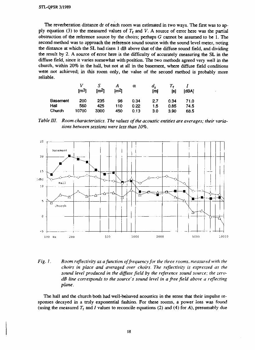
The reverberation distance dr of each room was estimated in two ways. The first was to ap- ply equation (3) to the measured values of T, and V. A source of error here was the partial obsuuction of the reference source by the choirs; perhaps G cannot be assumed to be 1. The second method was to approach the reference sound source with the sound level meter, noting the distance at which the SL had risen 1 dB above that of the diffuse sound field, and dividing the result by 2. A source of error here is the difficulty of accurately measuring the SL in the diffuse field, since it varies somewhat with position. The two methods agreed very well in the church, within 20% in the hall, but not at all in the basement, where diffuse field conditions were not achieved; in this room only, the value of the second method is probably more reliable.

Basement 200 235 96 0.34 2.7 0.34 71.0 Hall 560 425 110 0.22 1.5 0.85 74.5 Church 10700 3300 450 0.13 3.0 3.90 68.5

Table III. Room characteristics. The values of the acoustic entities are averages; their varia- tions between sessions were less than 10%.

Fig. 1. Room reflectivity as a function offrequency for the three rooms, nieasured with the choirs in place and averaged over choirs. The reflectivity is expressed as the sound level produced in the difluse field by the reference sound source; the zero- dB line corresponds to the source's sound level in a pee Beld above a reflecting plane.

The hall and the church both had well-behaved acoustics in the sense that their impulse re- sponses decayed in a truly exponential fashion. For these rooms, a power loss was found (using the measured T, and I values to reconcile equations (2) and (4) for A), presumably due

STL-QPSR 311989

to the choirs partially obstructing the reference source, as described above. The loss was just over 1 dB for all choirs in the church, and just under 2 dB in the hall. Removing half of the fan's output power would result in a loss of 3 dB, so these appear to be reasonable values. In the basement, a diffuse field was not achieved, so little accuracy could be expected. There were noticeable room resonances in this room, with low frequencies decaying much slower than high ones. For this room, reconciling equations (2) and (4) for A indicated a power loss of 5-6 dB, which seems unreasonably large.

With this reservation, Fig. 1 shows the diffuse field sound level of the reference noise in the three rooms, as a function of frequency. High values indicate a large amount of room reflec- tions. For each room, the curves are averages of two channels and three sessions, from which has been subtracted the power spectrum level of the reference noise source, as taken from the manufacturer's calibration chart. The 0-dB line therefore approximates the sound level of the reference noise source in the calibration condition, i.e. in a free field above a reflecting plane. The absorption characteristics were quite similar for the hall and the church, although the church was about 6 dB lower overall. The basement had a cluster of prominent resonances around 200 Hz. This uneven spectral distribution of the absorption was another aspect of the awkwardness of the acoustics in the basement.

2.2.3. Dynamic levels, songs, and radiation For each choir and each room, ten items were recorded in varying conditions, yielding a total of 90 items for LTAS analysis (Table IV). There were three conditions of vocal effort: pp, mf andfl. There were two conditions of music material: song A (Hark, the Herald Angels Sing) and song B (Jungfiun hon g&r i ringen). The boys' choir sang the soprano part in unison, while the other two choirs sang in the normal mixed settings. The [mf, song A] condition was re- peated once for assessing reproducibility, and once with the singers hiding their mouths from the conductor, using their usual size A4 hard binders containing the music. The actual order of conditions 2-7 was pseudo-randomized. Each item was of at least 30 seconds duration.

cal. pp mf mf repeat mf obstructed Background noise 1 Choir song A 2 3 4 8 9 Choir song B 5 6 7 Reference noise 10

Table N. Recording sequence of ten 30-second items. This sequence was performed with three choirs in three rooms, i.e. nine times altogether.

2.3. LTAS analysis The LTAS analyses were made using a unique real-time device, built by Johan Liljencrants, which is connected to a Data General S/140 minicomputer. It consists of a bank of 31 analog band-pass filters, arranged in third-octave bands from 20 Hz to 20 kHz. The filter outputs are scanned, processed and presented graphically by custom software.

LTAS printouts were made of the left and right channels of each item, making a total of 180 plots. From each plot the 31 filter levels were measured manually to the nearest half-decibel and entered into a software spreadsheet. The spreadsheet was used to apply filter level correc- tions and calibration offsets, and also to compute the various averages and to present graphics. The analyses of the choirs were restricted to the frequency range 0.1 - 10 kHz. There was little voice energy outside this range, and the calibration charts for the reference source extended no further.

3. RESULTS This section first discusses some possible sources of error. Then, because power levels and sound levels in the choirs are of great relevance to the general spectrum appearance, they are dealt with at some length. Finally, the LTAS effects of the experimental conditions are re- ported.

3.1. Background noise The background noise was measured with the choirs in place but silent. Low-frequency noise below 50 Hz from ventilation systems or traffic outside was always present. Its influence was minimal, however, since the A scale was used for weighting all full-band level measurements, and also because the noise never overlapped the range of vocal frequencies. Fig. 2 shows the LTAS of a typical choir item, including background noise, as well as the A frequency weight- ing characteristic.

Fig. 2 . Typical choir LTAS showing low-frequency background noise and the IEC-651 frequency weighting A-scale (right axis). The close agreement in LTAS for the two channels seen here was representative for all items. [Adult choir, Hall, song A, mfl

3.2. Reproducibility The LTAS from the two channels were typically within f 2 dB of each other over the entire

spectrum, for all choirs and all rooms (Fig. 2). This means that the positioning of the micro- phones was not very critical. All further LTAS results are averages of the two channels.

The LTAS of the reference noise was also reproducible between the three sessions to within -2 dB, even though the following factors were not strictly controlled: microphone positions, reference source position, and the number and position of the people in the room." The re- hearsal hall was an exception: for the youth choir session only, it had about 3 dB more ab- sorption in the high frequency range of 10-20 kHz. This could be due to the fact that the youth choir was the largest, and/or to some change in the position of curtains.

*Of particular concern was the unfortunate circumstance that the church, unknown to us, was sched- uled for its first renovation in many decades. On arriving for the second session, we found scaffolding here and there, and for the third session, the church was closed to the public, there was scaffolding everywhere, and most of the ceiling was obscured by gangplanks. We went ahead anyway, and fortu- nately, the changes had had little or no effect on the LTAS of the reference noise, or on the perceived acoustics.

For the duplicated condition [song A, mfl, all choirs reproduced their LTAS very closely. If allowance is made for slight variations in vocal output power, the LTAS remained typically within f 1 dB over the entire frequency range.

3.3. Sound power output of the choirs We consider first the overall output power of the choirs in the various conditions. Changes in the output power should reflect variations in the vocal effort, provided that the words and mu- sic remain the same. The average power produced by the choir during the thirty seconds in each condition was measured by comparing the equivalent (time-averaged) SL of the choir to the SL of the reference noise, whose power was known. For each condition, the equivalent SL was computed from the LTAS, which accumulates energy over time.

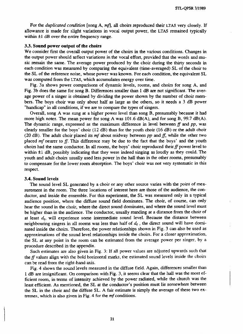
Fig. 3a shows power comparisons of dynamic levels, rooms, and choirs for song A, and Fig. 3b does the same for song B. Differences smaller than 1 & are not significant. The aver- age power of a singer is obtained by dividing the power shown by the number of choir mem- bers. The boys choir was only about half as large as the others, so it needs a 3 dB power "handicap" in all conditions, if we are to compare the types of singers.

Overall, song A was sung at a higher power level than song B, presumably because it had more high notes. The mean power for song A was 101.6 &(A), and for song B, 99.7 clB(A). The dynamic range, expressed as the maximum difference in level between ff and pp, was clearly smaller for the boys' choir (12 dB) than for the youth choir (16 dB) or the adult choir (20 dB). The adult choir placed its mf about midway between pp and ff, while the other two placed mf nearer to ff. This difference may be due to the fact that the boys' and the youth choirs had the same conductor. In all rooms, the boys' choir reproduced their ff power level to within f 1 dB, possibly indicating that they were indeed singing as loudly as they could. The youth and adult choirs usually used less power in the hall than in the other rooms, presumably to compensate for the lower room absorption. The boys' choir was not very systematic in this respect.

3.4. Sound levels The sound level SL generated by a choir or any other source varies with the point of mea-

surement in the room. The three locations of interest here are those of the audience, the con- ductor, and inside the ensemble. For this experiment, the SL was measured only in a typical audience position, where the diffuse sound field dominates. The choir, of course, can only hear the sound in the choir, where the direct sound dominates, and where the sound level must be higher than in the audience. The conductor, usually standing at a distance from the choir of at least d,, will experience some intermediate sound level. Because the distance between neighbouring singers in all rooms was less than half of dr , the direct sound will have domi- nated inside the choirs. Therefore, the power relationships shown in Fig. 3 can also be used as approximations of the sound level relationships inside the choirs. For a closer approximation, the SL at any point in the room can be estimated from the average power per singer, by a procedure described in the appendix.

Such estimates are also given in Fig. 3: If all power values are adjusted upwards such that the ff values align with the bold horizontal marks, the estimated sound levels inside the choirs can be read from the right-hand axis.

Fig. 4 shows the sound levels measured in the diffuse field. Again, differences smaller than 1 dB are insignificant. On comparison with Fig. 3, it seems clear that the hall was the most ef- ficient room, in terms of intensity achieved by the power radiated, while the church was the least efficient. As mentioned, the SL at the conductor's position must lie somewhere between the SL in the choir and the diffuse SL. A fair estimate is simply the average of these two ex- tremes, which is also given in Fig. 4 for the mf conditions.

Power [ d B ( h ) 1 Song A S L [d8 ( A ) I 1 w 1 2 0 r 1 0 5

1 B o y s ' c h o i r Youth c t ~ o i r A d u l t c t ~ o i l I

Fig. 3. Acoustic power produced by the choirs for song A (a) and song B (b). Rooms: B = basement, H=Hall, C=Church. Dynamic levels: white=pp, gray = m i black= ff. The approximate sound levels inside the choirs are given by the right-hand scale, provided that all columns are shifed upwards so that the ff columns align with the black markers.

Power [ d B ( A ) ] Song B S L [ d B ( h ) l

1W 1 2 0

1 1 5

1 U 5

Boys ' c h o i r Youth c h o l r A d u l t cli 1 1

- - 100

*mf cond

Song A

[dB (A) I S L

1 0 0

95

mf cond

[dB (A1 1 S L

Fig. 4 . Sound levels at a listening position in the diffuse field for song A (a) and song B (b). Rooms: B= basement, H=Hall, C=Church. Dynamic levels: white=pp, gray=mf, black=ff. White markers indicate the estimated mf SL at the conductor's position.

Boys' choir Youth choir Adult choir (a1

(b)

100 -

9 5

Boys' choir Youth choir Adult choir

STL-QPSR 311989

3.5. Long-time average spectra

3.5.1. Effect of vocal effort It is a well-known effect that the higher partials gain in amplitude more rapidly than the lower ones, as vocal output power increases (Fant, 1959; Gauffin & Sundberg, 1980). The spectrum variations arising from changes in dynamic level are typically like those shown in Fig. 5. The wealth of data gathered in this experiment enabled us to examine this effect in some detail. In the pp-mffdynamic range studied here, the relationship between a sound level change (in dB) and the resulting spectrum level change at any given frequency was found to be quite linear. This convenient circumstance prompts us to introduce a dimensionless, frequency-dependent gain factor g o , by which the overall sound level change may be multiplied in order to predict the spectrum level change at a given frequency.

Fig. 6 summarizes g(f) for the three choirs. Each point is an average of 12 observations of g atf The standard deviations, also shown, were mostly an order of magnitude smaller than the mean. It can be seen that a SL change of 10 dB typically resulted in a spectrum level change at 3 kHz of about 20 dB. This is in close agreement with the results of Fant (1959) for speech. The boys' choir, which sang in unison, did not sing below 250 Hz. AU curves pass through g=l at about 700 Hz, implying that this was the frequency at which the spectrum level covar- ied most closely with the A-weighted sound level. The youth choir was different from the other two choirs, in that its g factor was lower around 1200 Hz and higher at 3 kHz. The dif- ferences reached a significance level of 0.99.

3.5.2. Effect of musical material The two songs were compared by taking LTAS from the [song A, mfl and [song B, mfl condi- tions and averaging over the three rooms, for each choir. The principal difference found was around 1100 Hz, where the spectrum level for song A consistently was about 2 dB higher than song B. This might have been caused by the second formant of the vowel [a], which occurred more often in stressed positions in song A. The differences between song A and song B were however small for all choirs. If compensation is made for the slightly higher power levels used for song A, the difference in LTAS shape was typically less than 1 dB (i.e., as small as for the duplicate items), and never more than 3 dl3 at any frequency.

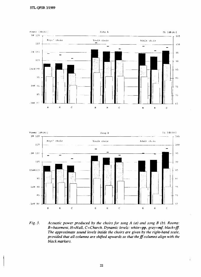
3.5.3. Effects of choir type A spectral comparison of choir types should be made for the same singer sound power.

Only the [Song B, 8, Hall] condition met this requirement for all choirs. A larger base for comparisons was created by choosing the [Song A, mfl conditions (including duplicates) for all rooms, subtracting the room characteristics, and creating one average LTAS per choir, scaled to show the power of one average singer in that choir. In the [Song A, mfl condition, the average youth singer had radiated 2 dB more power than the average adult, while the aver- age boy singer had radiated 1 dB less.

These three average LTAS were therefore normalized for power level at 700 Hz, at the same time correcting the spectrum slope using the g factors obtained in 3.5.1. In this way, we could compare the types of choir as though the singers had produced the same output power (Fig. 7). Interestingly, the youth and adult choir types were almost identical, the only difference being that the youth type put out about 3 dl3 more in the 1-2 kHz range. Singing in mf, both types had a spectrum slope of about -10 &/octave from 700 Hz to 4000 Hz, while the boy type had a slope of about -15 @/octave.

STL-QPSR 311 989

1 0 0 1000 Hz 10000

Fig. 5 . Example of LTAS effect of dyrlaniic levels. [Adult choir, hall, sortg A]

1 0 0 1 0 0 0 Hz 10000

.Boys m e a n O ~ o u t h m e a n *Adu l t m e a n ---Boys SD --- Youth SD -Adult SD

Fig. 6 . Gain factor g(f) suinnzarizing the r.elative spectrum level change observed for a giver1 sourtd level change. Each poirtt is a nzeait of 12 observations. Tlte standard deviatiorts are showrt as lines.

STL-QPSR 311989

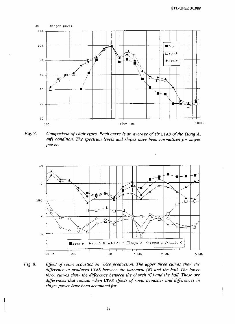
3.5.4. Effect of room acoustics on phonation The hall's acoustics were appointed as a norm to which the other rooms were compared. Since voice control is probably more precise in mf than in pp or ff, the average of the mf conditions was chosen as the subject of the comparisons. The influence of the room acoustics on the LTAS was cancelled by subtracting the appropriate room characteristic (Fig. 1). The known spectral effects of differences in vocal power (Fig. 3) were also accounted for, using the factor go de- scribed above. Above 5 kHz, the sound levels were sometimes low enough to be near the noise floor of the LTAS filter bank, so this frequency region was discarded. Fig. 8 shows the re- maining LTAS differences: the basement compared to the hall (filled markers), and the church compared to the hall (open markers). A change toward pressed phonation would appear as an increased spectrum slope; i.e. a reduced spectrum level at low frequencies and/or an increased spectrum level at high frequencies. Such an effect was found only for the boys' choir, whose normalized spectrum level in the basement relative to that in the hall was about 3 dB lower at low frequencies and 2 dB higher at high frequencies.

For all choirs, however, the difference curves for the basement have a markedly "bumpy" appearance, with peaks near 450, 800 and 2000 Hz, and with minima near 600, 1100, and 3000 Hz. These bumps are due to a general increase in formant frequencies, on the order of 5- 10% (as can be verified, e.g. by offsetting a curve from Fig. 5 by +lo% in frequency and comparing its levels to the original). Such an increase could be caused by a raised larynx: A high larynx implies a shorter vocal tract and therefore higher formant frequencies. Difference curves with identical "bumps" resulted when the author compared LTAS of himself singing with a high versus a low larynx. Hence it would appear that all the choirs were in fact singing with a higher larynx in the basement than in the hall. Similar LTAS differences were found for the pp andfi conditions.

The formant-shift effect, though weaker, was also visible in the church-to-hall comparison (lower half of Fig. 8). Here, the LTAS difference curve for the boys' choir looks very different from the other two. The reason is that the boys' choir, contrary to the other two choirs, sang with lower power in the church than in the hall, which effectively reverses the comparison. If the curve for the boys' choir is mirrored about the 0-dB line, it becomes similar to the other two.

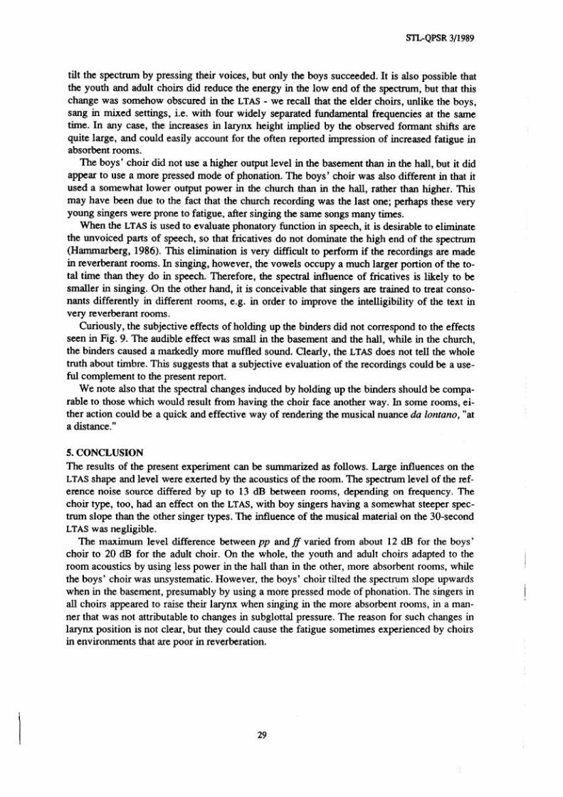
3.5.5. Effect of changing the sound propagation path In one condition, the singers held their binders containing the music about 30 cm in front of

the mouth, so that the conductor could see only the singers' eyes, while the singers could still read the music. The result of comparing this condition to that with the binders held down is shown in Fig. 9, with averages over all choirs for each of the three rooms. The effect was sim- ilar in all rooms, with a high-frequency loss of 1-3 dB in the 2-10 kHz range, and a 2-dB boost in the 200-500 Hz range.

Since the measurements were made in the diffuse sound field, the high-frequency loss is probably not due to obstruction of the direct sound, but rather to the circumstance that a larger portion of the voice output was reflected onto the body of the singer, there to be absorbed; and perhaps to absorption in the binders themselves. In the basement, the sound field was not quite diffuse, and hence the obstruction of the direct high-frequency sound path may have contributed, in addition to the other effects. This would explain why the basement gave the largest high-frequency loss. From Fig. 9, we can infer that the lack of diffuseness in the basement had LTAS effects which were limited to 1-2 dB in the frequency range 2-6 kHz. The boost in the upper bass region came as a surprise to the author. It may be due to resonance effects in the 'cavity' created between the binder and the body of the singer. The dimensions of such a cavity are on the order of half a wavelength at the frequencies of the boosted region.

dB S i n g e r power

Fig. 7. Conzparison of choir types. Each curve is an average of six LTAS of the [song A, mfl condition. The specrrunz levels and slopes have been rtornlalized for singer power.

100 Ilz 200 500 5 kHz

Fig. 8. Effect of room acoustics on voice production. Tlie upper three curves show the difference in produced LTAS betweeiz the basenlent (B) and the hall. The lowei. three curves show the difference between the church (C) and the hall. These are differences that remain when LTAS effects of roonz acoustics and differences in sirtgei power have been accounted for.

STL-QPSR 311989

Fig. 9. Effect on the diffuse field LTAS of holdirtg up the nzusic binders in front of the mouth. Average of all choirs. Altltough tile LTAS changes were similar in all three rooms, the subjective effect was quite different.

4. DISCUSSION The present experiment showed that with changes in the acoustical environment, the youth and adult choirs tended to change their vocal output level. These two choirs used higher levels in the basement and in the church than in the hall, thereby apparently compensating for room absorption. The concomitant changes in spectrum tilt would assist in compensating for the greater high-frequency absorption in the basement and the church. Furthermore, all choirs were found to use 5-10% higher formant frequencies in the basement than in the hall, a differ- ence which probably was caused by an increase in larynx height, on the order of 1 cm. Such a raise could be passively induced by higher subglottal pressure, or actively applied in order to achieve some change in the sound, or both. In Fig. 3a, it can be seen that the choirs sang with about 2 dB more power in the basement. Higher output power is achieved mostly with a higher subglottal pressure, which would tend to raise the larynx, especially at high effort lev- els. Because power is more or less proportional to subglottal pressure (Bouhuys & a1. 1968), we would expect the larynx shift and hence the foxmant shift to be larger in the ff conditions, and much smaller or absent in the pp conditions. how eve^. the fotma11t shift was ahout the same at all dynamic levels. This suggests that the change in 1;11ynx height was tiot primarily a side effect of changing the output power. but rather an active ctcljustn~ent.

For the youth and adult choirs, the change of room was not accornpanietl hy a change in spectrum tilt, other than that ascribable to a higher output level. This latter finding is consis- tent with those reported from a similar experiment on speech, with adult singer and non-singer subjects (Sundberg, Ternstrom, Perkins, & Grmning, 1988).

Why the choir singers would want to raise their larynx remains unclear. The spectral change thus achieved was small compared to the differences in room absorption. A raised lar- ynx is closely related to pressed phonation (Sundberg, 1989). Perhaps all choirs were trying to

STL-QPSR 311989

The spectrum-slope effects of changing the musical dynamic level were entirely as ex- pected. They were described in detail using a frequency-dependent gain factor. This factor was found to vary fiom about 0.5 at 200 Hz to 2 at 3 kHz, passing through 1 at about 700 Hz. The gain factor proved to be useful for normalizing the LTAS to different singer power levels. The frequency characteristic of the gain factor was similar but not identical for the three choirs.

Obstructing the sound propagation path with the music binders resulted in a 3 dB loss of treble but also in a 2 dB boost in the upper bass region. The subjective effect of this change was very different in different rooms.

Acknowledgments This experiment was made in collaboration with the department of Logopedics and Phoni- atrics, Karolinska Institute, Huddinge University Hospital. It was greatly facilitated by the ex- tensive and enthusiastic assistance of Anita Huhn and Ulrika Josephson, logoped students at the said department, for whom this work was a thesis project. I owe them many thanks. The participation of the choirs of Jacobs Kyrka (St. James's Church), Stockholm, is gratefully acknowledged. The department of Technical Acoustics at KTH kindly lent us the reference sound source. I am indebted to Johan Sundberg for his valuable comments on the manuscript. This investigation is part of the project "Analysis and Synthesis of Choral Sound," which is generously supported by the Bank of Sweden Tercentenary Foundation.

References Bouhuys, A., Mead, J., Proctor, D.F. & Stevens, K.N. (1968): "Pressure-flow events during singing," Annals of the New York Academy of Sciences 155, Article 1, pp. 165-176.

Fant, G. (1959): "Acoustic analysis and synthesis of speech with applications to Swedish," Ericsson Technics No. 1, 1959.

Gauffin, J. & Sundberg, J. (1980): "Data on the glottal voice source behavior in vowel production," STL-QPSR 2-3/1980, pp. 61-70.

Hammarberg, B. (1986): Perceptual and Acoustic Analysis of Dysphonia, Ph.D. thesis, Karolinska In- stitute, Stockholm 1986.

Kitzing, P. (1 986): "LTAS criteria pertinent to the measurement of voice quality," J. Phonetics 14, pp. 477-482.

Kuttruff, H. (1979): Room Acoustics, 2nd edition. Applied Science Publishers, London.

Lubman, D. (1974): "Precision of reverberant sound power measurements," J. Acoust. Soc. Am. 56:2, pp. 523-533. Marshall, A.H. & Meyer, J. (1985): "The directivity and auditory impressions of singers," Acustica 58, pp. 130-140.

Sundberg, J. (1987): The Science of the Singing Voice, Northern Illinois University Press, DeKalb, Illi- nois, USA.

Sundberg, J. (1989). Personal communication.

Sundberg, J., Ternstrom, S., Perkins, W.H., & Gramming, P. (1988): "Long-term average spectrum analysis of phonatory effects of noise and filtered feedback," J. of Phonetics 16, pp. 203-219.

STL-QPSR 311989

Using the symbols given in Table 11, the sound intensity I generated in a room by a source at a distance d is given by

where the first tern pertains to the direct sound and the second term to the reverberating sound (c.f. Kuttruff). Assuming that we have a choir with N members, each radiating the same power w, the total intensity at a given point in the room becomes

where di is the distance to singer i and Gi is the directional gain factor of singer i as seen at the listening position. The fust term is a bit cumbersome in practice. The intensity of the direct sound contributed by all N singers can however be approximated by the direct sound intensity from an equivalent number ne of singers, all at the same equivalent distance de. Assuming that G averages to 1 for an arbitrary listening position, the direct-sound term becomes

and we need only to estimate n, and de. For an audience position, clearly n, = N, while de is the distance to the choir. If the singers are fairly close to and facing the audience, we should also include G with a value of about 2 in the numerator. For a position inside the choir, the di- rect sound is dominated by the nearest neighbours. If the choir is standing in two rows, most singers have five neighbours, at an equivalent distance de which may be computed as the in- verse of the RMS of the inverted neighbour distances di, i.e.

The singers are facing in various directions relative to the point of interest, so let us ap- proximate G to 1. The direct sound intensity contribution of the remaining singers will usually be equivalent to only one or two more immediate neighbours, depending on the size of the choir. Hence we can estimate the sound intensity level experienced by a silent, monaural lis- tener inside the choir using the expression

where ne is typically 6 and de varies but is on the order of 0.8 m.