numerical modelling in seismic analysis of...

FACTA UNIVERSITATIS

Series: Architecture and Civil Engineering Vol. 11, No 3, 2013, pp. 251 - 267 DOI: 10.2298/FUACE1303251Z

NUMERICAL MODELLING IN SEISMIC ANALYSIS OF

TUNNELS REGARDING SOIL–STRUCTURE INTERACTION

UDC 624.19:624.042.7=111

Elefterija Zlatanović1#

, Gordana Broćeta2, Nataša Popović-Miletić

2

1University of Niš, Faculty of Civil Engineering and Architecture, Serbia

2University of Banjaluka, Faculty of Architecture and Civil Engineering,

Republic of Srpska, Bosnia and Herzegovina #[email protected]

Abstract. The paper is related to the most significant aspects of numerical simulations

in seismic analysis of tunnels, highlighting the soil–structure interaction phenomenon.

The modelling of a problem and analysis of relevant influences may be completed by

an application of software packages based on the finite element method. In order to

define a reliable and efficient numerical model, that should simultaneously put

together both the criteria of simplicity and realistic presentation of a physical problem,

analyses should start from the most simple modelling techniques (theory of elasticity,

replacing the soil medium with elastic springs, pseudo-static analysis), with the final

goal to accomplish a more complex and realistic model (theory of elasto-plasticity,

finite element method, full dynamic analysis).

Key words: tunnel, earthquake, soil–structure interaction, finite element model

1. INTRODUCTION

A simplified approach for the seismic design of tunnels is aimed to provide a tool for

estimating the earthquake-induced stress increments in the tunnel lining [1]. Although it

may be simple, it should be able to capture the most significant aspects of the seismic re-

sponse of tunnels, including their lining and the surrounding ground, the seismic excita-

tion should be properly represented, and the effects of dynamic soil–structure interaction

should be properly accounted for. In order to apply the finite element method (FEM) con-

cepts, certain assumptions and idealizations must be made. It is necessary to specify soil

behaviour in the form of a mathematical constitutive relationship, as well as to simplify

and/or idealize the geometry and/or boundary conditions of the problem. To a first ap-

Received December 5, 2013 Acknowledgement: The authors gratefully acknowledge the support of the Ministry of Education, Science

and Technological Development of Serbia within the Project TR36028 (2011–2014).

E. ZLATANOVIĆ, G. BROĆETA, N. POPOVIĆ-MILETIĆ

252

proximation the transversal response may be considered to be uncoupled from the longi-

tudinal response (i.e., the response along the direction of the tunnel axis).

2. GEOMETRIC IDEALIZATION – 2D VS. 3D ANALYSIS

Wave scattering and complex three-dimensional wave propagation can lead to differ-

ences in wave amplitudes along the tunnel, since ground motion incoherence tends to in-

crease the strains and stresses in the longitudinal direction. Although the use of 3D meth-

ods to study dynamic soil–structure interaction under earthquake excitation has the appeal

that some of the modelling errors are reduced, it suffers from the important disadvantages

that the solution time and the complexity of the analysis are substantially increased. It is

therefore necessary to make some rational approximations related to 2D analyses that may

be performed within reasonable time period. Plane strain model in modelling three-di-

mensional tunnel structures should be adopted when they are uniform throughout their

length (homogeneous surrounding medium, ground motion coherence, as well as continu-

ous cast-in-place and straight-jointed segmented linings), or without considering defor-

mation of the tunnel face and staggered-jointed lining rings.

In a 2D analysis there can be used plane strain and axi-symmetric approach depend-

ing on the desirable results. The plane strain approach can be used when analyzing shal-

low tunnels and the effects of the surface settlements, or to study the effects of tunnel con-

struction on existing structures. In addition, the plane strain analyses can be used when

transverse sections of multiple tunnels are modelled. The axi-symmetric approach is

widely used for deep tunnels, when the surface settlements are not of prime interest or

when the face advance is analyzed. Moreover, there are two methods of seismic response

analysis, frequency domain analysis and time domain analysis.

3. BOUNDARY CONDITIONS

In infinite systems, wave that propagates to infinity does not bounce back to the soil

(structure) model. In numerical simulations, attention is usually restricted to a finite region.

Then an artificial boundary condition is needed to make the computational domain finite. In

addition, for computational efficiency, it is desirable to minimize the number of elements in

a finite-element analysis, by minimizing the size of the discretized region. As the size of the

discretized region decreases, the influence of boundary conditions becomes more significant.

3.1. Uniform ground vs. two-layered formation

Under the assumption of uniform ground (infinite elastic or elasto-plastic space), the

influence of ground surface is ignored. This approach is being used for deeply buried tun-

nel structures, considering P- and S-wave propagation. Since the overburden of the tun-

nel is too thick and the ground surface cannot be modelled, the outer boundaries should

be located at distances several times the tunnel diameter (4–5D), which should be far

enough from the tunnel such that the presence of boundaries does not affect the solution.

It could result in reducing the errors of stresses up to several percent.

Numerical Modelling in Seismic Analysis of Tunnels Regarding Soil–Structure Interaction

253

Under the assumption of two-layered formation (semi-infinite elastic or elasto-plastic

space), the influence of the ground surface is considered. This approach is being used for

shallow embedded tunnel structures, in which case, beside P and S body waves, surface

R-waves have a significant contribution to the response of tunnel structures. The effect of

the truncated soil medium is generally approximated by the artificial boundary such as a

horizontal plane located under the bottom of the tunnel, at the bedrock along which the

forces are being applied to the model. This boundary condition causes propagation of

stress and strain waves upwards, due to which the tunnel stability against these stresses

and strains should be estimated. In the case of two-layered formation (soft soil overlying

bedrock), and vertically propagating shear waves, for determining maximum layer thick-

ness to avoid filtering of relevant frequencies, following relation should be satisfied:

max4 f

sC

H (1)

where Cs is the S-wave velocity of the soil layer, and fmax is the natural frequency of the

soil at which the strongest amplification occurs. The greatest amplification factor will

occur at the lowest natural frequency, also known as the fundamental frequency.

3.2. Simulation of rigid and elastic bedrock

The boundary condition at the bottom of the soil deposit depends on the nature of the

underlying bedrock that could be assumed as a rigid boundary or elastic boundary.

If the bedrock is rigid, its motion will be unaffected by motions in the overlying soil.

It acts as a fixed-end boundary. Any downward-traveling waves in the soil will be

completely reflected back toward the ground surface by the rigid layer, thereby trapping

all of the elastic wave energy within the soil layer. In a time domain analysis, the rigid

bedrock is simply modelled by imposing an acceleration (or velocity or displacement)

time-history at the base of the numerical model (its particle acceleration can be specified

directly as the input motion to the lower boundary of the FE mesh) [2].

If the bedrock is elastic, downward-traveling stress waves that reach the soil–rock

boundary will be reflected only partially; part of their energy will be transmitted through

the boundary to continue traveling downward through the rock and thus effectively

removed from the soil layer. This is a form of radiation damping, and it causes the free

surface motion amplitudes to be smaller than those for the case of rigid bedrock. In a time

domain analysis, the presence of an elastic bedrock can be modelled by imposing a force

time history rather than a base motion at the bottom of the soil layer (earthquake input

motion cannot be imposed at viscous boundary). The continuity of the stresses along the

rock–soil boundary requires that shear stress at the bottom of the soil layer be equal to the

shear stress at the top of the rock. For this reason, the motion of an elastic bedrock is

usually specified by adopting a shear stress time history τ(t) [3].

3.3. Simulation of silent boundaries in infinite media

For problems involving wave propagation analysis, the usual finite boundary of the

finite element model will cause the elastic waves to be reflected and superimposed with

the progressing waves. To avoid these reflections, it is necessary to impose a special


254

MEVP

)1)(21(

)1(

GEs

V

)1(2

condition on the restraining boundary, which is perfectly radiating to outgoing waves and

transparent to incoming waves. Such boundary conditions have a variety of names, such

as absorbing, silent, anechoic, non-reflecting, transmitting, radiating, transparent, or one-

way boundary conditions.

The viscous damping boundary method (VDB) uses the concept of applying viscous

dampers to the DOF on the boundary element. For an elastic media, such as soil, there are

primary waves and secondary waves that travel through the media. Primary waves are

compression waves that travel through solids, liquids, and gases. Secondary waves are

shear waves that only travel through solids. The boundary condition is [4]:

waveSecondary

waveSecondary

wavePrimary

ySyz

xSzx

zPzz

uVb

uVb

uVa

(2)

These equations are formulated for incident primary and secondary waves that act at an

angle ζ from the z-axis as shown in Fig. 1. In the above equations, ρ is a density, G is a

shear modulus, and M is a constraint modulus of the media, u x, u y, u z represent the

velocities in the x,y,z-direction, VP and VS are the velocities of the primary and secondary

waves, and a, b are relaxation coefficients. For small incident angles (ζ<30°), the most

effective value for the dimensionless parameters a and b is 1.0.

The concept of the perfectly matched layers method (PML) [4] is designed to

absorb thoroughly any incident wave without reflection, for any incident angle, and at any

frequency before discretization. The main concept is to surround the computation domain

at the infinite media boundary with a highly absorbing boundary layer, as shown in Fig. 2.

The objective of the PML method is to construct a new wave equation that creates plane

waves that decay exponentially in the PML in the direction of the PML:

λi = 1 iγ (3)

Here γ is the attenuation in the PML region. This value will be zero in the computational

domain. The complex coordinate stretching function λ is continuous.

In the concept of infinite elements, the basic idea is to place elements with a special

shape function for the geometry at the infinite boundary. Therefore, there will be two sets

of shape functions, the standard shape functions (N) and a growth shape functions (M).

The growth shape functions (M) grow without limit as coordinate approaches infinity, and

are applied to the geometry. The standard shape functions (N) are applied to the field

variables. The geometry of the element (Fig. 3) is interpolated as [4]:

x = M1x1 + M2x2

1

21M

1

12M (4)

This yields x = x1 at ξ = −1, x = x2 at ξ = 0 and

1

)1(2

1lim 21

3

xxx .


255

Fig. 1 Viscous Damping Fig. 2 PML surrounds Fig. 3 Example of

Boundary [4] the domain [4] Infinite Element [4]

There are other solutions for silent boundaries: the energy transmission boundary,

the roller boundary (under horizontal ground motion, the vertical fixed and horizontal

free hinge bearings are being used), and the periodical boundary [5]. Special boundary

conditions for wave propagation in saturated porous media are also proposed [6].

4. DISCRETIZATION CONSIDERATIONS

For plane strain conditions, the model is being discretized by triangular or

quadrilateral finite elements, forming the FE unstructured or structured mesh. The mesh,

on one hand, should be fine enough in order to accomplish more realistic results, but on

the other hand, it should not be time and computational consuming due to a large number

of nodes. A simple way to determine if the element size is fine enough to produce good

results is by solving the problem with a certain number of elements and then comparing

its results to the results of a model with twice as many elements. If a substantial difference

between the results of the two models is detected, then the mesh refinement is necessary

[7]. The finer mesh should be taken around the tunnel, where there are areas of highly

stress concentration, in order to increase the accuracy of the analysis (Fig. 4).

In dynamic FEM analysis, the response of FE models can be influenced by

discretization. In particular, the use of coarse finite-element meshes can result in the

filtering of high-frequency components whose short wavelengths cannot be modelled by

widely spaced nodal points. The maximum dimension of any element should be limited to

one-eighth of the shortest wavelength considered in the analysis [8].

Fig. 4 Finite element mesh in numerical Fig. 5 Dynamically imposed displacements

model – smaller elements in areas at a random node, for the uniform

of high stress concentration ground analysis [10]

5. GROUND MOTION SIMULATION

To obtain the acceleration time histories many options are available including artificial,

spectrum-compatible accelerograms, synthetic records generated by a seismological model of


256

the source, and real accelerograms (i.e., true records). The use of real accelerograms is

preferred; however it is influenced by two problems: the lack of ground motion recordings in-

depth, and the difficulty to adequately scale the time-histories recorded at the free surface.

5.1. Harmonic function of ground motion

Harmonic loading is usually being used in order to understand fundamental charac-

teristics of the dynamic behaviour of the tunnel, when the model is excited by sinusoidal

waves ( t sin0 , tieVV 0 ). After that, the analysis is followed by earthquake

simulation as the exciting seismic waves [9].

When using a harmonic input to the model, according to recommendations of Kou-

retzis et al. [10], the buildup of ground motion should be gradual (Fig. 5), using a transi-

tion time interval equal to 8 wave periods, so as numerical pseudo-oscillations from the

sudden application of a large amplitude displacement to be avoided.

5.2. Real earthquake records

In order to better simulate an earthquake, a real acceleration record should be taken as

a dynamic input. Usually, two types of earthquake ground motions are being considered

in the seismic response analysis of structures: an earthquake ground motion with a high

probability of occurrence for structures in service, and an earthquake ground motion with

a low probability but having a large acceleration. Recently, it is very often practice as the

source of dynamic excitation the acceleration record for the 1995 Kobe, Japan earthquake

to be used, as shown in Fig. 6, because this earthquake was the most devastating to civil

infrastructure in recorded history.

The duration of strong ground motion can have a strong influence on earthquake dam-

age. Many physical processes, such as the degradation of stiffness and strength of certain

types of structures, and the buildup of pore water pressures in loose saturated sands, are

sensitive to the number of load or stress reversals that occur during an earthquake. A motion

of short duration may not produce enough load reversals for damaging response to build up

in a structure, even if the amplitude of the motion is high. On the other hand, a motion with

moderate amplitude but long duration can produce enough load reversals to cause substantial

damage. The duration of strong motion increases with increasing earthquake magnitude.

Fig. 6 Acceleration record of the 1995 Fig. 7 The bracketed duration of

Kobe Earthquake in Japan an earthquake ground motion [3]

An earthquake accelerogram generally contains all accelerations from the time the

earthquake begins until the time the motion has returned to the level of background noise.


257

For engineering purposes, only the strong-motion portion of the accelerogram is of inter-

est. To save on the computer CPU time, the recorded motion could be truncated before

and after the certain periods. Different approaches have been taken to the problem of

evaluating the duration of strong motion in an accelerogram. Because it implicitly reflects

the strength of shaking, the bracketed duration is most commonly used for earthquake

engineering purposes. The bracketed duration is defined as the time between the first and

last exceedances of threshold acceleration (usually 0.05g) (Fig. 7).

5.3. Synthetic records

In the lack of real earthquake records, artificial ground motions must be developed.

The main challenges in their development are to ensure that they are consistent with the

target parameters (peak accelerations, velocities, or spectral ordinates) and that they are

realistic. This is not as easy as it might appear; many motions that appear reasonable in

the time domain may not when examined in the frequency domain, and vice versa. Many

reasonable time histories of acceleration produce, after integration, unreasonable time

histories of velocity and/or displacement. The methods for generation of artificial ground

motions are [3]: (a) modification of actual ground motion records, (b) generation of artifi-

cial motions in the time domain, (c) generation of artificial motions in the frequency do-

main, and (d) generation of artificial motions using Green's function techniques.

The simplest approach is the modification of actual recorded ground motions.

Maximum motion levels, such as peak acceleration and peak velocity, could be used to

rescale actual strong motion records to higher or lower levels of shaking (Fig. 8). A de-

sirable ground motion record will have not only a peak acceleration or velocity close to

the target value, but also magnitude, distance, and local site characteristics that are similar

to those of the target motion. Such a record is most likely to have a similar frequency

content and duration to the target motion. Rescaling of the time scale may be used to

modify the frequency content of an actual ground motion record. This is usually accom-

plished by multiplying the time step of a digitized actual record by the ratio of the pre-

dominant period Tp (corresponding to the maximum value of the Fourier amplitude spec-

trum) of the target motion to the predominant period of the actual motion (Fig. 9).

Fig. 8 (a) Original accelerogram from actual Fig. 9 (a) Original accelerogram from

actual earthquake; (b) rescaled version actual earthquake; (b) rescaled version

of original accelerogram (accelerations of original accelerogram (time

scaled upward by a factor of 1.5 scale scaled upward by a factor of

to match target peak acceleration) [3] 1.3 to match target predominant

period; the duration has also been

increased by a factor of 1.3) [3]


258

6. MODELLING METHODS FOR SURROUNDING SOIL/ROCK MEDIUM

There are two basic approaches in modelling the soil/rock medium surrounding a

tunnel structure: a spring supported approach (discontinuous model, discrete model) in

the scope of conventional models, i.e., models based on subgrade reaction, and a FEM

approach (continuous model).

6.1. Beam–spring / shell–spring approach (bedded beam models)

A spring model is used to express the interface between structure and soil, when a set

of a structure and ground layers are simultaneously analyzed in order to evaluate the

effects of soil–structure interaction (Fig. 10). In a seismic analysis, the interaction

between the ground and the tunnel in plane strain conditions is being simulated by a

coupled-type interaction spring consisting of a radial and tangential ground spring.

Seismic forces acting on the beam–spring model can be assumed to be the product of

ground displacements, ground shear stress, and inertial force, according to the Seismic

Deformation Method (Fig. 11). The ground displacements are applied at the end of the

ground springs, whereas the ground shear stresses are applied directly to the lining [9].

Fig. 10 Simplified three-dimensional Fig. 11 Concept of the Seismic

beam–spring model for soil – Deformation Method

tunnel structure analysis using beam–spring model

Linear (elastic) springs are used for the linear behaviour of the soil. In order to take

into account the nonlinear behaviour of the soil, the use of nonlinear springs with bilinear

elasto-plastic behaviour could be used, with an aim to add hysteretic damping to springs.

A spring–dashpot model should be used when viscosity is considered; forces are

generated due to the difference in velocity of the structure and the ground (Fig. 12).

Fig. 12 Elastic spring, elasto-plastic spring, and Kelvin–Voigt elements

When using simple numerical models such as the beam–spring model, only a single

structure can be accommodated in the analysis. They do not provide information on


259

overall (global) stability or on movements in the adjacent soil, and ignore soil shearing

transferring effects on adjacent structures and services.

6.2. FEM approach (continuous soil models)

One of the great benefits of numerical analysis to the tunnel engineer is that an analy-

sis with FEM soil modelling can incorporate adjacent influences (existing surface struc-

tures, tunnels, etc.).

6.2.1. Elastic soil models

With regard to linear isotropic elasticity, an isotropic material is one that has point

symmetry, i.e., every plane in the body is a plane of symmetry for material behaviour.

Only two independent elastic constants are necessary to represent the behaviour. In

structural engineering it is common to use Young's modulus, E', and Poisson's ratio, μ'.

For geotechnical purposes, it is often more convenient to characterize soil behaviour in

terms of the elastic shear modulus, G, and effective bulk modulus, K'.

Soil/rock rarely behaves as a linear elastic material. The simplest approach would be

to model them as a nonlinear elastic material. Two methods may be used to construct a

nonlinear elastic stress–strain relation. They are known as Green's hyperelastic theory and

hypoelastic theory. There are: the bi-linear model, K–G model, and the Dancan–Chang

hyperbolic model [11]. Nonlinear elastic models, in which the material parameters vary

with stress and/or strain level, are a substantial improvement over their linear counter-

parts. Due to the number of parameters involved, most nonlinear elastic models assume

isotropic behaviour. However, they still fail to model some of the important facets of real

soil behaviour. They cannot reproduce the tendency to change volume when sheared.

Also, because of the inherent assumption of coincidence of principal incremental stress

and strain directions, they cannot accurately reproduce failure mechanisms.

6.2.2. Equivalent-linear soil models

Experimental results have suggested some energy to be dissipated even at a very low

strain level, thus indicating that the damping ratio of a soil is never zero. It is also sug-

gested that both the soil shear modulus and the damping ratio are dependent on the shear

strain level. To describe the degradation of the shear modulus and the increase of the

damping ratio along with the shear strain level increase, different curves were proposed in

the literature for various types of soils [3]: fine-grained soils, sand, and gravel (Fig. 13).

These are equivalent linear soil models that represent only an approximation of the actual

nonlinear behaviour of the soil. For that reason they are not proposed to be used directly

for problems concerning permanent ground deformation or failure, because they imply

that the strain always returns to zero after the cyclic loading. Consequently, since a linear

material has no limiting strength, it is not possible to achieve the soil failure. And yet, the

assumption of linearity allows a very efficient class of constitutive models to be used for

ground response analyses, particularly for problems involving low strain levels such as

stiff soil deposits and weak input motions.


260

Fig. 13 Equivalent-linear model for Fig. 14 Cyclic nonlinear soil model:

sand after Seed and Idriss [12] (a) variation of shear stress with time;

(b) resulting stress–strain behaviour

(backbone curve indicated by dashed line) [3]

6.2.3. Cyclic nonlinear soil models

The nonlinear behaviour of soils can be represented more accurately by cyclic nonlin-

ear models that follow the actual stress–strain path during cyclic loading. They are char-

acterized by a backbone curve, rules that govern unloading–reloading behaviour, stiffness

degradation, and many other effects (Fig.14). A variety of cyclic nonlinear soil models

has been proposed [3]: the hyperbolic model, the modified hyperbolic model, the Ram-

berg–Osgood model, the Iwan-type model, the nonlinear hysteretic model – Iwan and

Mroz IM model, the Martin–Davidenkov model, the Cundall–Pyke model, the Hardin–

Drnevich–Cundall–Pyke model (HDCP), etc. Hashash and Park [13] introduced an exten-

sion of the modified hyperbolic model to capture the dependence of shear modulus deg-

radation and damping curves on the confining pressure.

6.2.4. Elasto-plastic soil models

The most accurate and general methods for representation of soil behaviour are based

on elasto-plastic soil models. These models use the basic principles of mechanics to de-

scribe the true soil behaviour under initial stress conditions, a wide variety of stress paths,

rotating principal stress axes, monotonic or cyclic loading, low or high strain levels, and

undrained or drained conditions. They are characterized by a yield surface that represents

the limiting stress conditions, a hardening/softening law that describes changes in the size

and shape of the yield surface along with an occurrence of plastic deformation, and a flow

rule that relates plastic strain increments to stress increments. The simplest of these mod-

els are simple elasto-plastic models (Fig. 15) such as: the Tresca (1864) and von Mises

models for cohesive soils, the Mohr–Coulomb and Drucker–Prager (1952) models for co-

hesive frictional soil or rock, the Hoek–Brown model (1980) for rock masses, the Lade–

Duncan model (1975), and the Matsuoka–Nakai model (1974, 1982) [11, 14]. More com-

plex advanced constitutive models are critical state models that incorporate the Cam-clay

(1963) and modified Cam-clay (1968) models for cohesive soils [11], as well as the

CASM model for both clay and sand [14]. The most complex are advanced elasto-plastic

models with multiple yield and plastic potential surfaces: the Lade’s double hardening

model, the MIT-E1 and MIT-E3 soil models, and the bubble models [11]. Advanced con-


261

stitutive models allow significant generality and flexibility in simulating the response of

soils under cyclic loading conditions. Nevertheless, for their description many more pa-

rameters than needed for the equivalent linear or cyclic nonlinear models are usually re-

quired. Evaluation of these parameters can be quite complex, and their values obtained from

one type of test can considerably differ from those obtained from another. Although the

application of advanced constitutive models has undoubtedly been increased, these practical

issues have so far limited their use in geotechnical earthquake engineering practice.

Fig. 15 Comparison of simple elastic perfectly plastic models [11]

7. SOIL DAMPING FORMULATION

The frequency domain (FD) solution of wave propagation provides the exact

solution when the soil response is linear. For a linear elastic material, the area bounded by

stress–strain loops is zero and then, there is no hysteretic damping. However, laboratory

tests have clearly shown the presence of damping at very small strains, too. Numerically,

this problem can be overcome by introducing viscous dashpots embedded within linear

elastic elements. Soil behaviour is approximated as a Kelvin–Voigt solid.

Homogeneous linear visco-elastic layer the wave equation becomes independent of

frequency for a harmonic loading with a circular frequency ω. Since the solution for an

arbitrary loading is performed by transforming the motion into a finite sum of harmonic

motions using the Fourier transform, the damping of the system becomes independent of

the frequency of the input motion due to the frequency independent viscosity:

G2

(5)

1. If the viscosity ε is constant, amplification function will have only finite number of

peaks, corresponding to those natural frequencies of the layer which have damping less

than critical. A critical value of viscosity can be established for each particular mode:

Gn

H

)12(

4

, n=1, 2, … (6)

Constant value of viscosity corresponds to an increasing percentage of damping ξ in each

mode, meaning that the amplitude of the peak at the second natural frequency of the layer

will be 1/9 of that at the first, the amplitude at the third will be 1/25, etc. (Fig. 16, left).

2. If it is assumed that viscosity is inversely proportional to the frequency, so that

εω/(2G) is constant, it corresponds to constant damping ξ in all modes. In this case, the

amplitude of second peak will be 1/3 that of the first, the amplitude of the third peak 1/5,

and so on (Fig. 16, right).


262

Fig. 16 Amplification curve for uniform layer over rigid rock:

(left) constant viscosity; (right) constant modal damping [15]

In nonlinear analysis, the dynamic equation of motion is integrated in the time

domain (TD) and the nonlinear soil behaviour can be accurately modelled. Soil damping

is captured primarily through the hysteretic energy dissipation. Viscous damping, using

the Rayleigh damping formulation, is often added to represent damping at very small

strains where many soil models are primarily linear. The Rayleigh damping formulation

results in frequency dependent damping, in contrast to experiments that show that the

damping of soil is mostly frequency independent. An appropriate choice of frequency

range is needed.

Early Rayleigh formulations used a simplified form of the damping matrix, which is

only stiffness proportional and depends only on the first mode of the deposit:

][][ KC R (7)

where βR = 2ξ / ω1 and ω1 is the frequency of the first natural mode of the soil column.

The contribution of higher modes is small for relatively short soil columns, but may

become important for deeper soil columns and for high frequency motion [16].

Conventional Rayleigh formulation (CRF) is a double frequency method. In the

original damping formulation proposed by Rayleigh and Lindsay in 1945, the [C] matrix

is assumed to be proportional to the mass and stiffness matrices:

][][][ KMC RR (8)

It is a common practice to choose frequencies that correspond to the first mode and the

second mode of the soil column, or the first mode of the soil column and a higher mode

that corresponds to the predominant frequency of the input motion. This formulation may

underestimate or overestimate the ground motion response at high frequencies, and the

accuracy of solution deteriorates with an increase in depth of soil column [17].

In Rayleigh formulation (RF), the performance of the double frequency RF analysis is

improved by a different selection of the two significant frequencies. They should be

selected in part to cover the range of significant frequencies in the input motion.

Equation (8) can be extended, so that more than two frequencies/modes (usually four)

can be specified, and is referred to as extended Rayleigh formulation (ERF) [17]. The

effective damping is illustrated in Fig.17, assuming the damping ratios are equal at the

selected frequencies/modes.


263

Fig. 17 Effective (frequency dependent) Fig. 18 Hybrid beam–shell FEM model [21]

damping using RF and ERF

damping formulations [17]

8. MODELLING THE TUNNEL LINING

Tunnels linings are composed by materials which are more uniform than the ground,

and are mostly assumed elastic [18]. In addition, in soil–structure interaction analysis, one

of key influential parameters is a stiffness of a tunnel lining [1].

8.1. Continuous cast-in-place tunnel lining

This section is listing possibilities for suitable FE modelling of a tunnel lining

composed of conventional concrete or self compacting concrete (SCC) [19]. Using solid

elements has a significant drawback as the need to maintain an acceptable element shape

(defined by the aspect ratio of length to width). A tunnel lining is likely to be very thin

relative to the tunnel diameter and boundary distance. Moreover, this option cannot reveal

the distribution of bending moments, axial and shear forces. There is a possibility to use

structural elements. The beam model can be based on Bernoulli–Euler theory and

Timoshenko beam theory. Shell elements are appropriate to be used where the structure is

in presence of the membrane stress combined with bending stresses. The shells can be

conventional or continuum ones. In the case of underground structures at crossings with

active strike-slip faults, the hybrid beam–shell FEM model [20, 21] has been proposed

(Fig. 18). The length of affected pipeline under fault movements is usually too long for a

shell-mode calculation because of the limitation of memory and costly computations.

Therefore, only the pipeline segment near fault is modelled with large deformation shell

elements in order to consider the effect of large section deformation, and then beam

elements are used to model far-fault parts of the pipeline. For reinforced linings, the bars

can be accounted in the model by modifying the bulk properties of the lining.

8.2. Prefabricated (jointed, segmented) tunnel lining

The lining of a TBM driven (shield) tunnel consists of single precast concrete

segments which are assembled at the ring (coupling, circumferential, lateral) joints and

segment (longitudinal) joints. Segments are bolted together in the tangential direction to

form rings, and the rings are bolted together in longitudinal direction to form the tunnel

lining. Presence of joints could result in up to 50% reduction in the developed moments


264

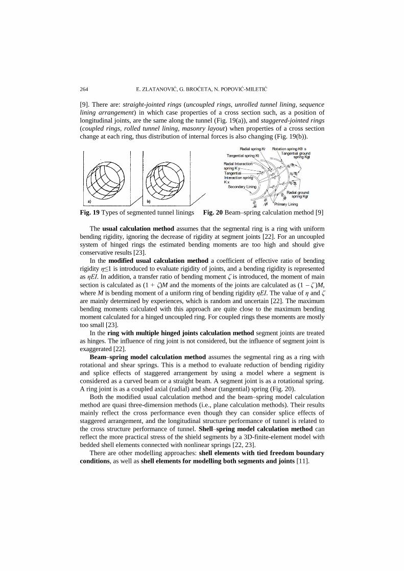
[9]. There are: straight-jointed rings (uncoupled rings, unrolled tunnel lining, sequence

lining arrangement) in which case properties of a cross section such, as a position of

longitudinal joints, are the same along the tunnel (Fig. 19(a)), and staggered-jointed rings

(coupled rings, rolled tunnel lining, masonry layout) when properties of a cross section

change at each ring, thus distribution of internal forces is also changing (Fig. 19(b)).

Fig. 19 Types of segmented tunnel linings Fig. 20 Beam–spring calculation method [9]

The usual calculation method assumes that the segmental ring is a ring with uniform

bending rigidity, ignoring the decrease of rigidity at segment joints [22]. For an uncoupled

system of hinged rings the estimated bending moments are too high and should give

conservative results [23].

In the modified usual calculation method a coefficient of effective ratio of bending

rigidity ε≤1 is introduced to evaluate rigidity of joints, and a bending rigidity is represented

as εEI. In addition, a transfer ratio of bending moment δ is introduced, the moment of main

section is calculated as (1 + δ)M and the moments of the joints are calculated as (1 δ )M,

where M is bending moment of a uniform ring of bending rigidity εEI. The value of ε and δ

are mainly determined by experiences, which is random and uncertain [22]. The maximum

bending moments calculated with this approach are quite close to the maximum bending

moment calculated for a hinged uncoupled ring. For coupled rings these moments are mostly

too small [23].

In the ring with multiple hinged joints calculation method segment joints are treated

as hinges. The influence of ring joint is not considered, but the influence of segment joint is

exaggerated [22].

Beam–spring model calculation method assumes the segmental ring as a ring with

rotational and shear springs. This is a method to evaluate reduction of bending rigidity

and splice effects of staggered arrangement by using a model where a segment is

considered as a curved beam or a straight beam. A segment joint is as a rotational spring.

A ring joint is as a coupled axial (radial) and shear (tangential) spring (Fig. 20).

Both the modified usual calculation method and the beam–spring model calculation

method are quasi three-dimension methods (i.e., plane calculation methods). Their results

mainly reflect the cross performance even though they can consider splice effects of

staggered arrangement, and the longitudinal structure performance of tunnel is related to

the cross structure performance of tunnel. Shell–spring model calculation method can

reflect the more practical stress of the shield segments by a 3D-finite-element model with

bedded shell elements connected with nonlinear springs [22, 23].

There are other modelling approaches: shell elements with tied freedom boundary

conditions, as well as shell elements for modelling both segments and joints [11].


265

8.3. Sprayed concrete lining

The lining model presented in the previous section can also be applied to the modelling

of sprayed concrete linings being used in NATM – New Austrian Tunnelling Method. There

are no segments and joints, but the entire lining uses this special model, so cracking is

permitted to develop at any location around the lining, particularly if severe distortions of the

tunnel lining such under the earthquake action are expected [24].

8.4. Composite concrete lining (primary and secondary lining)

The parts of linings are modelled as beams. To model internal transmission of

sectional forces between the linings, an interlayer modelled by a plane strain element is

installed between the beams used to simulate the primary and secondary lining [25]. An

alternative approach to model the interface between the primary and secondary lining is

by the radial and tangential interaction springs (Fig. 20) [9]. In the analysis of El Naggar

et al. [26], the tunnel lining is treated as an inner jointed thin-walled shell coupled with

an outer continuous thick-walled cylinder embedded in elastic ground. The outer thick-

walled cylinder can be used to simulate composite liner behaviour (e.g., tunnel supports

comprising a primary and secondary lining), or to consider the influence of a degraded

zone around the inner tunnel lining.

9. MODELLING THE CONTACT INTERFACE

Interface between structural elements and soil can be modelled in a variety of ways

[11]. The use of continuum elements, with compatibility of displacements, in a finite el-

ement analysis prohibits relative movement at the soil–structure interface (no-slip condi-

tion). In many soil–structure interaction situations, however, relative movement of the

structure with respect to the soil can occur, i.e. slip and even separation, excluding the oc-

currence of penetrating an element into adjacent one (full-slip condition). Many methods

have been proposed to model discontinuous behaviour at the soil–structure interface: thin

continuum elements with standard constitutive laws; linkage elements in which only the

connections between opposite nodes are considered (usually opposite nodes are con-

nected by discrete springs); special interface or joint elements of either zero or finite

thickness; hybrid methods where the soil and structure are modelled separately and

linked through constraint equations to maintain compatibility of force and displacement at

the interface. Full slip condition could also be modelled through a ring of plane strain

elements with a very low shear modulus G [27]. The most accurate simulation of the

soil–structure interface is by using the surface-to-surface contact model.

10. CONCLUDING REMARKS

The finite element method is used lately to solve complex problems regarding tunnel

structures such as: simulating the construction sequences, realistic soil behaviour,

complex hydraulic conditions, accounting for adjacent structures, short and long term

conditions, multiple tunnels, seismic behaviour. Although it is considered the most exact

calculation method, in the FEM the input data dictate the resulting output, and can be


266

"wrong" even if the algorithm works properly. The modelling is subjected to six sources

of errors that might lead to poor predictions: modelling the geometry of the problem,

modelling of construction method and its effects, constitutive modelling and parameter

selection, theoretical basis of the solution method, interpretation of results, human error.

It is important to understand the behaviour of each finite element and their limitations, in

order to choose the right solution for the interaction between a tunnel structure and soil.

REFERENCES

1. Zlatanović, E., "Influence оf earthquakes оn the stress and strain state of the shallow tunnel structures in

saturated soil of low bearing capacity", Facta Universitatis: Architecture and Civil Engineering 6(2),

2008, pp. 221-227.

2. Visone, C., Santucci de Magistris, F. and Billota, E., "Comparative study on frequency and time domain

analyses for seismic site response", EJGE, Vol. 15, 2010.

3. Kramer, S. L., Geotechnical Earthquake Engineering, Prentice Hall, New Jersey, 1996.

4. Ross, M., "Modelling methods for silent boundaries in infinite media", ASEN 5519-006: Fluid-Structure

Interaction, Aerospace Engineering Sciences – University of Colorado at Boulder, 2004.

5. Uno, K., Shiojiri, H., Kawaguchi, K. and Nakamura, M., "Analytical method, modelling and boundary

condition for the response analysis with nonlinear soil-structure interaction", 14th WCEE, Beijing,

China, 2008.

6. Gajo, A., Saetta, A., Vitaliani, R., "Silent boundary conditions for wave propagation in saturated porous

media", International Journal for Numerical and Analytical Methods in Geomechanics, Vol. 20, 1996,

pp. 253-273.

7. Moaveni, S., Finite Element Analysis: Theory and Application with ANSYS, Pearson Education, NJ, 2003.

8. Kuhlemeyer, R. L. and Lysmer, J., "Finite element method accuracy for wave propagation problems",

Journal of the Soil Mechanics and Foundations Division, ASCE, 99(5), 1973, pp. 421-427.

9. Mizuno, K. and Koizumi, A., "Dynamic behavior of shield tunnels in the transverse direction

considering the effects of secondary lining", 1st European Conf. on Earthq. Engin. and Seismology,

Geneva, Switzerland, 2006.

10. Kouretzis, G. P., Bouckovalas, G. D. and Gantes, C. J., "3-D shell analysis of cylindrical underground

structures under seismic shear (S) wave action", Soil Dynamics and Earthquake Engineering 26, 2006,

pp. 909-921.

11. Potts, D. M. and Zdravkovic, L., Finite Element Analysis in Geotechnical Engineering: Theory, Thomas

Thelford, London, 1999.

12. Bardet, J. P., Ichii, K. and Lin, C. H., "EERA – A computer program for Equivalent-linear Earthquake

site Response Analyses of layered soil deposits", University of Southern California, Los Angeles,

California, 2000.

13. Hashash, Y. M. A. and Park, D., "Non-linear one-dimensional seismic ground motion propagation in the

Mississipi embayment," Engineering Geology 62, 2001, pp. 185-206.

14. Yu, H.-S., Plasticity and Geotechnics, Springer Science + Business Media, LLC, New York, 2006.

15. Milutinović, Z., Engineering Seismology, International Postgraduate Program IZIIS Master Course,

2007-2008.

16. Hashash, Y. M. A. and Park, D., "Viscous damping formulation and high frequency motion propagation

in non-linear site response analysis", Soil Dynamics and Earthquake Engineering 22, 2002, pp. 611-624.

17. Park, D. and Hashash, Y. M. A., "Soil damping formulation in nonlinear time domain site response

analysis," Journal of Earthquake Engineering 8(2), 2004, pp. 249-274.

18. Yue, Q. X. anf Li, J., "Dynamic response of utility tunnel during the passage of Rayleigh waves", 14th

World Conference on Earthquake Engineering, Beijing, China, 2008.

19. Broćeta, G., "Istraživanje komponentnih materijala samozbijajućeg betona sa metodama ispitivanja

svježe betonske mase", Magistarski rad, Arhitektonsko-graĊevinski fakultet, Univerzitet u Banjaluci,

Banjaluka, 2010.

20. Karamitros, D. K., Bouckovalas, G. D. and Kouretzis, G. P., "Stress analysis of buried steel pipelines at

strike-slip fault crossings", Soil Dynamics and Earthquake Engineering 27, 2007, pp. 200-211.


267

21. Halabian, A. M., Hokmabadi, T. and Hashemolhosseini, S. H., "Numerical study on soil-HDPE pipeline

interaction subjected to permanent ground deformation", 14th WCEE, Beijing, China, 2008.

22. Huang, Z., Zhu, W., Liang, J., Lin, J. and Jia, R., "Three-dimensional numerical modelling of shield

tunnel lining", Tunnelling and Underground Space Technology 21, 2006, pp. 434.

23. Klappers, C., Gruebl, F. and Ostermeier, B., "Structural analysis of segmental lining – coupled beam and

spring analysis versus 3D-FEM calculations with shell elements", Tunnelling and Underground Space

Technology 21, 2006, pp. 254-255.

24. Potts, D. M. and Zdravkovic, L., Finite Element Analysis in Geotechnical Engineering: Application,

Thomas Thelford, London, 2001.

25. Karinski, Y. S., Shershnev, V. V., Yankelevsky, D. Z.,"The effect of an interface boundary layer on the

resonance properties of a buried structure", Earthquake Engineering and Structural Dynamics 33, 2004,

pp. 227-247.

26. El Naggar, H., Hinchberger, S. D. and El Naggar, M. H., "Simplified analysis of seismic in-plane

stresses in composite and jointed tunnel linings," Soil Dynamics and Earthquake Engineering 28, 2008,

pp. 1063-1077.

27. Corigliano, M., Lai, C. G. and Barla, G., "Seismic response of rock tunnels in near-fault conditions," 1st

European Conference on Earthquake Engineering and Seismology, Geneva, Switzerland, 2006, Paper

No. 998.

NUMERIĈKO MODELIRANJE U SEIZMIĈKOJ ANALIZI

TUNELA SA ASPEKTA INTERAKCIJE KONSTRUKCIJE I TLA

U radu su istaknuti najznačajniji aspekti numeričkog modeliranja u seizmičkoj analizi tunela,

sa posebnim osvrtom na fenomen interakcije konstrukcije sa okolnim tlom. Modeliranje problema i

analiza relevantnih uticaja mogu se izvršiti primenom softvera baziranih na metodu konačnih

elemenata. U cilju definisanja pouzdanog i efikasnog numeričkog modela, koji istovremeno treba

da obuhvati kriterijume jednostavnosti i realistične prezentacije fizičkog problema, u analizama

treba poći od jednostavnijih tehnika modeliranja (teorija elastičnosti, modeliranje okolnog tla

elastičnim oprugama, pseudo-statička analiza) kako bi se postigao kompleksniji i realističniji

model (teorija elasto-plastičnosti, metod konačnih elemenata, dinamička analiza).

Kljuĉne reĉi: tunel, zemljotres, interakcija konstrukcije i tla, model sa konačnim elementima.

numerical modelling in seismic analysis of...

Documents