numerical modelling of the seismic behaviour of adobe buildings
DESCRIPTION
PhD thesis, Numerical model of adobe structuresTRANSCRIPT
Università degli Studi di Pavia Istituto Universitario di Studi Superiori
Numerical modelling of the seismic behaviour of adobe
buildings
A Thesis Submitted in Partial Fulfilment of the Requirements
for the Degree of Doctor of Philosophy in
EARTHQUAKE ENGINEERING
by
Sabino Nicola Tarque Ruíz
December, 2011

Università degli Studi di Pavia Istituto Universitario di Studi Superiori
Numerical modelling of the seismic behaviour of adobe
buildings
A Thesis Submitted in Partial Fulfilment of the Requirements
for the Degree of Doctor of Philosophy in
EARTHQUAKE ENGINEERING
by
Sabino Nicola Tarque Ruíz
Supervisors:
Prof. Enrico Spacone, Università degli Studi ‘Gabriele D’Annunzio’ Chieti-Pescara
Prof. Humberto Varum, University of Aveiro
Co-supervisors:
Prof. Guido Camata, Università degli Studi ‘Gabriele D’Annunzio’ Chieti-Pescara
Prof. Marcial Blondet, Pontificia Universidad Católica del Perú
December, 2011

ABSTRACT
In this research, the possibility to numerical describing the seismic behaviour of adobe constructions through finite element models is studied. Principally, two experimental tests were reproduced: a cyclic in-plane test on an adobe wall and a dynamic test on an adobe module, both carried out at the Pontificia Universidad Católica del Perú, Peru, where the thesis’ author have participated. The state-of-the-art for the numerical modelling of unreinforced masonry point to three main approaches: macro-modelling, simplified micro-modelling and detailed micro-modelling. The first one related to continuum models and the last two approaches are related to discrete models. In all three approaches, the use of elastic and inelastic parameters is required. For adobe masonry, the lack of knowledge concerning some of the material mechanical properties, especially in tension and shear, makes numerical modelling more difficult.
The results of tests on adobe blocks (i.e. compression strength, elasticity modulus, shear strength), as well as the results of cyclic and dynamic tests on adobe masonry components and adobe modules show that the mechanical properties of adobe masonry highly depend on the type of soil used for the production of units and mortar. Basic properties, such as elasticity modulus, can have significant variation from one soil type to another. The adobe material is characterized as a brittle material; it has acceptable compression strength but it is poor regarding tensile and shear strength.
Here, the mechanical properties of the adobe masonry used in the model for the simulation of the cyclic in-plane experimental response were calibrated to match well the global lateral strength-deformation response of the adobe wall and its crack pattern evolution. The adobe masonry studied is representative of the Peruvian adobe constructions. Macro-modelling (smeared crack and damaged plasticity models) and simplified micro-modelling (discrete model) strategies were used in finite element software with an implicit solution strategy. After verification of the results it was preliminary concluded that a macro-modelling strategy could be used for adobe masonry. The lack of accurate material properties for the mud mortar joints ends with convergence problems when dealing with the simplified micro-modelling.
Then, the dynamic test of an adobe module was reproduced with a continuum model (damaged plasticity model) following an implicit and an explicit solution strategy, and using the material properties derived in the calibration. The comparison in terms of relative displacements and crack patterns in all the adobe walls studied showed a good agreement between the numerical and experimental results. Also, it was seen that an explicit solution strategy could be beneficial for analyzing adobe constructions due to its improvement in the calculation speed.
The result of this work is a benchmark for the numerical analysis of adobe walls under seismic actions. Since the adobe masonry can be considered as a homogeneous material, the macro-modelling (continuum model) approach, based on a damaged plasticity model, is a good option for modelling adobe structures. Finally, the proposed material parameters for numerical modelling predict well the adobe walls seismic capacity and the damage evolution. Therefore, the proposed mechanical parameters and methodology for numerical analyses could be used for modelling more complex configurations of unreinforced adobe walls: historical and vernacular.
Key words: non-linear finite element analysis, adobe masonry, material properties, discrete and continuum models, seismic analysis.
ACKNOWLEDGEMENTS
I would like to express my thanks to God and to all my family for being my support at every moment wherever I am. To my parents, Pilar and Sabino, and to my sister Ximena for encouraging me to continue in my studies and work, even when it took me far from home.
My gratitude goes to my advisor Dr. Enrico Spacone and co-supervisors Dr. Guido Camata, Dr. Humberto Varum and Dr. Marcial Blondet for their support, patience and useful suggestions and guidance throughout this research work.
I would also like to express my thanks to my colleagues and friends from the Civil Engineering Division of the Pontificia Universidad Católica del Perú for placing all the data from numerous tests carried out at the Structural Engineering Laboratory at my disposal. I am especially grateful to Prof. Julio Vargas and to Claudia Cancino for their productive preliminary discussions that improved the quality of this research.
Last but not least, I want to express my gratitude to all the people from around the world that I have met here in Italy, and especially to my friends from Collegio A. Volta and C. Golgi in Pavia; to Angelo N., Eleonora S., Luigi C. and Maria F. from Pescara; and to my colleagues from ASDEA (Pescara), for their kind help and humor throughout the good and difficult times that we have shared.

TABLE OF CONTENTS
ABSTRACT ...................................................................................................................................................v
ACKNOWLEDGEMENTS.....................................................................................................................vii
TABLE OF CONTENTS.......................................................................................................................... ix
LIST OF FIGURES ...................................................................................................................................xv
LIST OF TABLES....................................................................................................................................xxv
1. INTRODUCTION ..................................................................................................................................1
1.1 GENERAL ............................................................................................................................................1
1.2 JUSTIFICATION....................................................................................................................................2
1.3 ASSUMPTIONS .....................................................................................................................................2
1.4 OBJECTIVES ........................................................................................................................................3
1.5 THESIS OUTLINE.................................................................................................................................3
2. ADOBE HOUSES IN PERU ................................................................................................................7
2.1 GENERALITIES ...................................................................................................................................7
2.2 EVOLUTION OF THE ADOBE CONSTRUCTION IN PERU [VARGAS ET AL. 2005] ......................10
2.3 SEISMIC BEHAVIOUR OF UNREIFNORCED AND REINFORCED ADOBE STRUCTURES ...............14
2.3.1 The simple earth material, unreinforced adobe structures .............................................14
2.3.2 Seismic behaviour of unreinforced adobe houses...........................................................14
2.3.3 The earthquake-resistant reinforced adobe buildings .....................................................21

Sabino Nicola Tarque Ruiz
x
2.4 SUMMARY.......................................................................................................................................... 27
3. EXPERIMENTAL TESTS ON ADOBE MATERIAL ................................................................. 29
3.1 COMPRESSION TESTS ON ADOBE CUBES ...................................................................................... 29
3.2 COMPRESSION TESTS ON ADOBE PRISMS...................................................................................... 30
3.2.1 Specimens............................................................................................................................. 30
3.2.2 Testing .................................................................................................................................. 31
3.2.3 Results................................................................................................................................... 31
3.3 DIAGONAL COMPRESSION TEST ON ADOBE WALLETS ............................................................... 34
3.3.1 Specimens............................................................................................................................. 34
3.3.2 Testing .................................................................................................................................. 34
3.3.3 Results................................................................................................................................... 35
3.4 STATIC SHEAR WALL TESTS ............................................................................................................ 37
3.4.1 Specimens............................................................................................................................. 37
3.4.2 Tests ...................................................................................................................................... 38
3.4.3 Results................................................................................................................................... 39
3.5 CYCLIC TESTS ................................................................................................................................... 39
3.5.1 Specimens............................................................................................................................. 39
3.5.2 Tests ...................................................................................................................................... 42
3.5.3 Results................................................................................................................................... 43
3.5.4 Evaluation of the elasticity modulus................................................................................. 45
3.6 DYNAMIC TESTS............................................................................................................................... 50
3.6.1 Specimens............................................................................................................................. 50
3.6.2 Shake table description....................................................................................................... 52
Numerical modelling of the seismic behaviour of adobe buildings
xi
3.6.3 Test ........................................................................................................................................53
3.6.4 Results. ..................................................................................................................................55
3.7 SUMMARY ..........................................................................................................................................60
4. REVIEW OF NUMERICAL MODELS APPLIED TO MASONRY STRUCTURES.............63
4.1 FROM MICRO-MODELLING TO MACRO-MODELLING...................................................................63
4.2 FINITE ELEMENT APPROACHES FOR MASONRY MODELLING ....................................................69
4.2.1 Fracture mechanics approach: discrete model (micro-modelling) ................................70
4.2.2 Continuum mechanics approach: plasticity and damage mechanics (macro modelling) .........................................................................................................................................71
4.3 EXAMPLES OF NUMERICAL MODELLING ON MASONRY PANELS ...............................................73
4.4 SUMMARY ..........................................................................................................................................78
5. DISCRETE AND CONTINUUM MODELS FOR REPRESENTING THE SEISMIC BEHAVIOUR OF MASONRY.........................................................................................................79
5.1 REVIEW OF THEORY OF PLASTICITY..............................................................................................79
5.1.1 Fundamentals .......................................................................................................................80
5.1.2 Yield criterion.......................................................................................................................80
5.1.3 Flow rule ...............................................................................................................................82
5.1.4 Hardening/softening behaviour ........................................................................................83
5.2 DISCRETE MODEL: COMPOSITE CRACKING-SHEARING-CRASHING MODEL ............................85
5.2.1 Two-dimensional interface model .....................................................................................87
5.2.2 Three-dimensional interface model...................................................................................93
5.3 SMEARED CRACK MODEL: DECOMPOSED-STRAIN MODEL ........................................................95
5.3.1 Uncracked state material.....................................................................................................96
5.3.2 Cracked state material .........................................................................................................96
Sabino Nicola Tarque Ruiz
xii
5.3.3 Crack fracture parameters .................................................................................................. 98
5.4 SMEARED CRACK MODEL: TOTAL-STRAIN MODEL ..................................................................... 99
5.4.1 Compressive behaviour with lateral cracking ................................................................ 100
5.5 DAMAGED PLASTICITY MODEL ................................................................................................... 100
5.5.1 Strain rate decomposition ................................................................................................ 101
5.5.2 Stress-strain relations ........................................................................................................ 101
5.5.3 Hardening variables .......................................................................................................... 102
5.5.4 Yield function .................................................................................................................... 103
5.5.5 Damage and stiffness degradation under uniaxial condition....................................... 105
5.6 COMPRESSION AND TENSION CONSTITUTIVE LAWS................................................................. 109
5.6.1 Compression models ........................................................................................................ 109
5.6.2 Tension models ................................................................................................................. 110
5.7 SUMMARY........................................................................................................................................ 111
6. NON-LINEAR PSEUDO-STATIC ANALYSIS OF ADOBE WALLS................................... 113
6.1 IMPLICIT SOLUTION METHOD FOR SOLVING QUASI-STATIC PROBLEMS ................................ 113
6.2 DISCRETE MODEL: MODELLING THE PUSHOVER RESPONSE OF AN ADOBE WALL.............. 115
6.2.1 Calibration of material properties ................................................................................... 117
6.2.2 Results of the pushover analysis considering a discrete model................................... 124
6.3 TOTAL-STRAIN MODEL: MODELLING THE PUSHOVER RESPONSE........................................... 126
6.3.1 Calibration of material properties ................................................................................... 128
6.3.2 Results of the pushover analysis considering a total-strain model ............................. 132
6.4 CONCRETE DAMAGED PLASTICITY: MODELLING THE PUSHOVER RESPONSE. ..................... 135
6.4.1 Results of the pushover response considering the concrete damaged plasticity model 137
Numerical modelling of the seismic behaviour of adobe buildings
xiii
6.5 CONCRETE DAMAGED PLASTICITY: MODELLING THE CYCLIC BEHAVIOUR .........................139
6.5.1 Calibration of stiffness recovery and damage factors ...................................................140
6.6 VIBRATION MODES ........................................................................................................................152
6.7 ENERGY BALANCE FOR QUASI-STATIC ANALYSIS ......................................................................154
6.8 SUMMARY ........................................................................................................................................155
7. NON-LINEAR DYNAMIC ANALYSIS OF AN ADOBE MODULE ....................................157
7.1 SOLUTION APPROACHES FOR SOLVING DYNAMIC PROBLEMS .................................................157
7.1.1 Governing equations .........................................................................................................157
7.1.2 Implicit analysis..................................................................................................................159
7.1.3 Explicit analysis ..................................................................................................................160
7.2 IMPLICIT FINITE ELEMENT ANALYSIS OF THE ADOBE MODULE .............................................162
7.2.1 Model 1 ...............................................................................................................................164
7.2.2 Model 2 ...............................................................................................................................166
7.2.3 Model 3 ...............................................................................................................................167
7.2.4 Model 4 ...............................................................................................................................167
7.2.5 Model 5 ...............................................................................................................................169
7.2.6 Model 6 ...............................................................................................................................170
7.2.7 Model 7 ...............................................................................................................................172
7.2.8 Model 8 ...............................................................................................................................173
7.3 EXPLICIT FINITE ELEMENT ANALYSIS.........................................................................................175
7.3.1 Model 9 ...............................................................................................................................176
7.3.2 Model 10 .............................................................................................................................178
7.3.3 Model 11 .............................................................................................................................179
Sabino Nicola Tarque Ruiz
xiv
7.3.4 Model 12............................................................................................................................. 180
7.3.5 Model 13............................................................................................................................. 182
7.4 VIBRATION MODES ....................................................................................................................... 186
7.5 ENERGY BALANCE ........................................................................................................................ 189
7.6 SUMMARY........................................................................................................................................ 190
8. SUMMARY AND CONCLUSIONS ............................................................................................... 193
REFERENCES ........................................................................................................................................ 199
APPENDIX A. Comparison of the experimental and numerical relative displacement response of the adobe module. Implicit analysis............................................................................ 211
APPENDIX B. Comparison of the experimental and numerical total acceleration response of the adobe module. Implicit analysis. ........................................................................................... 221
APPENDIX C. Comparison of the experimental and numerical relative displacement response of the adobe module. Explicit analysis............................................................................ 231
APPENDIX D. Comparison of the experimental and numerical total acceleration response of the adobe module. Explicit analysis. ........................................................................................... 237
LIST OF FIGURES
Figure 2.1. Map of earthen constructions around the world................................................................8
Figure 2.2. Typical Peruvian adobe houses. ...........................................................................................8
Figure 2.3. Construction process of a tapial wall [Minke 2005]...........................................................9
Figure 2.4. Construction process of a quincha panel. .........................................................................10
Figure 2.5. Drawing of the ancient Caral city built in adobe..............................................................10
Figure 2.6. Temple of Pachacamac, ancient temple built in adobe. .....................................................11
Figure 2.7. Chan-Chan city (Trujillo, Peru). .........................................................................................11
Figure 2.8. Views of Carabayllo church. ...............................................................................................12
Figure 2.9. Colonial adobe houses of two and three storeys in Lima, Peru.....................................13
Figure 2.10. A vernacular adobe house located in Cusco (Peru) with no adequate geometrical configuration [Vargas et al. 2006]. .................................................................13
Figure 2.11. Destruction of adobe houses due to earthquakes. ...........................................................15
Figure 2.12. Vertical crack at the corner of an adobe house produced during the Pisco earthquake in 2007, Peru. ....................................................................................................16
Figure 2.13. Collapse of adobe houses during the Pisco earthquake in 2007, Peru. .........................16
Figure 2.14. Diagonal cracks produced in the adobe houses located at block corners, Pisco earthquake 2007....................................................................................................................17
Figure 2.15. Typical X-shape cracks on adobe walls due to in-plane actions. ...................................17
Figure 2.16. Configuration of typical roofs of adobe houses located in Pisco, Peru. .......................18
Figure 2.17. Seismic deficiencies on adobe masonry [CENAPRED 2003]. ......................................18
Sabino Nicola Tarque Ruiz
xvi
Figure 2.18. Typical failure damage on adobe masonry according to Dowling [2004].....................20
Figure 2.19. Typical types of damage observed in historic adobe buildings after the Northridge earthquake [Webster and Tolles 2000]..........................................................21
Figure 2.20. Internal cane mesh reinforcement. ....................................................................................22
Figure 2.21. Adobe models after seismic tests at the Pontificia Universidad Católica del Perú [Ottazzi et al. 1989]......................................................................................................23
Figure 2.22. External wire mesh reinforcement.....................................................................................24
Figure 2.23. Existing adobe buildings with external wire mesh reinforcement.................................24
Figure 2.24. External plastic (geogrid) mesh reinforcement. ...............................................................25
Figure 2.25. Adobe model reinforced with plastic mesh. .....................................................................26
Figure 2.26. Sketch of the prototype model of the scaled adobe module [Tolles and Krawinkler 1990]. .................................................................................................................27
Figure 3.1. Dry process of adobe bricks. ..............................................................................................29
Figure 3.2. Compression test on an adobe prism. ...............................................................................31
Figure 3.3. Stress-strain curves for axial compression tests on adobe prisms (modified from Blondet and Vargas [1978]). F-1 and F-2 refers to the lateral deformeters, while F-3 refers to the upper deformeters.................................................33
Figure 3.4. Scheme of the diagonal compression test (modified from NMX-C-085-ONNCCE [2002])................................................................................................................34
Figure 3.5. Diagonal compression tests on adobe wallets. .................................................................35
Figure 3.6. Scheme of the adobe walls for static shear test carried out by Blondet and Vargas [1978]. .......................................................................................................................38
Figure 3.7. Scheme of the adobe walls for static shear test carried out by Vargas and Ottazzi [1981] .......................................................................................................................38
Figure 3.8. Adobe walls for static shear tests [Blondet and Vargas 1978]........................................39
Figure 3.9. Adobe walls subjected to the cyclic test. ...........................................................................40
Figure 3.10. Scheme of the adobe walls for cyclic test [Blondet et al. 2005]. .....................................40
Numerical modelling of the seismic behaviour of adobe buildings
xvii
Figure 3.11. Scheme of the reinforced concrete ring beams [Blondet et al. 2005].............................41
Figure 3.12. Detail of load application and instrumentation on the adobe walls [Blondet et al. 2005]..................................................................................................................................41
Figure 3.13. Load application history for the cyclic tests......................................................................42
Figure 3.14. Hysteretic curves and crack pattern of the adobe walls subjected to the cyclic tests [Blondet et al. 2005; 2008]. All the right figures refer to the end of the cyclic tests. .............................................................................................................................44
Figure 3.15. Envelope of the hysteretic curves (positive and negative branch) from the cyclic tests. .............................................................................................................................45
Figure 3.16. Scheme for evaluating the lateral stiffness of the adobe wall I-1...................................47
Figure 3.17. Estimation of effective flange widths in structural walls (modified from Paulay and Priestley [1992]). ............................................................................................................49
Figure 3.18. Scheme of the adobe module subjected to a dynamic test [Blondet et al. 2005]..........50
Figure 3.19. Views of the adobe module subjected to the dynamic test.............................................51
Figure 3.20. Position of accelerometers and LVDTs on the adobe module......................................52
Figure 3.21. Horizontal acceleration record from May 1970 Peruvian earthquake, component N08W, registered in Lima. .............................................................................53
Figure 3.22. Views of the adobe module during and after the dynamic test......................................54
Figure 3.23. Displacement input at the base, Phase 1. ..........................................................................55
Figure 3.24. Relative displacement history during Phase 1...................................................................56
Figure 3.25. Total acceleration history during Phase 1. ........................................................................57
Figure 3.26. Displacement input at the base, Phase 2. ..........................................................................58
Figure 3.27. Relative displacement history during Phase 2...................................................................58
Figure 3.28. Total acceleration history during Phase 2. ........................................................................59
Figure 3.29. Rotation history between Right and Left Wall during Phase 2. .....................................60
Figure 4.1. Modelling strategies for masonry structures (modified from Lourenço [1996])..........64
Sabino Nicola Tarque Ruiz
xviii
Figure 4.2. Masonry failure mechanisms [Lourenço 1996]. ...............................................................65
Figure 4.3. Composite yield surface model proposed by Lourenço [1996]. ....................................66
Figure 4.4. Test scheme and sequence of loads of the masonry wall analyzed by Lourenço [1996]. ....................................................................................................................................67
Figure 4.5. Experimental crack patterns for different masonry walls analyzed by Lourenço [1996]. ..................................................................................................................67
Figure 4.6. Comparison of experimental and analytical pushover curves [Lourenço 1996]. .........68
Figure 4.7. Analysis of Kuçuk Ayasofya Mosque (Istanbul) by Roca et al. [2010] following a macro modelling approach...............................................................................................69
Figure 4.8. Concrete crack models [Midas FEA v2.9.6 2009]. ..........................................................69
Figure 4.9. Stress-displacement diagrams for quasi brittle materials [Lourenço 1996]...................70
Figure 4.10. Constitutive law for masonry composite (stress-strain curves)......................................71
Figure 4.11. Orthogonal crack models [Midas FEA v2.9.6 2009]. ......................................................72
Figure 4.12. Analysis of numerical results of an unreinforced masonry wall made by Lotfi and Shing [1994]. ..................................................................................................................73
Figure 4.13. Finite element discretization of masonry infill [Stavridis and Shing 2010]...................74
Figure 4.14. Comparison of pushover curves analyzed by Stavridis and Shing [2010]. ...................74
Figure 4.15. Numerical failure pattern of the masonry infill wall analyzed by Stavridis and Shing [2010]. .........................................................................................................................75
Figure 4.16. Mohr Coulomb with tension cut-off inelastic failure surface [Attard et al. 2007].......................................................................................................................................75
Figure 4.17. Modelling of masonry units by Attard et al. [2007]. .........................................................76
Figure 4.18. Experimental test and analytical approach of an URM building [Yi 2004]. .................77
Figure 4.19. Solid spandrel-cracked pier perforated URM wall model [Yi 2004]..............................78
Figure 5.1. Representation of a general yield surface (modified from Saouma [2000])..................81
Figure 5.2. Failure criteria for biaxial stress state illustrated for plane stress state (Modified from Jirasek and Bažant [2002]).......................................................................81
Numerical modelling of the seismic behaviour of adobe buildings
xix
Figure 5.3. Representation of associated and non-associated flow rule [Roca et al. 2010]. ............83
Figure 5.4. Movement of the yield surfaces. 1 and 2 are the principal stresses (modified from Cruz et al. [2004]). .....................................................................................84
Figure 5.5. Normal and tangential relative traction and displacement in 2D. .................................85
Figure 5.6. Normal and tangential relative traction and displacement in 3D. .................................85
Figure 5.7. Simplified representation of bricks and mortar joints into a numerical model [Lourenço 1996]. ..................................................................................................................86
Figure 5.8. Numerical and experimental shear behaviour of mortar joints reported by Lourenço [1996]. ..................................................................................................................90
Figure 5.9. Numerical and experimental tensional behaviour of mortar joints reported by Lourenço [1996]. ..................................................................................................................91
Figure 5.10. Hardening/softening compression law for masonry [Lourenço 1996].........................93
Figure 5.11. Three-dimensional interface yield function (modified from Midas FEA v2.9.6 [2009]). ...................................................................................................................................94
Figure 5.12. Decomposition of strains [Lotfi and Espandar 2004]....................................................95
Figure 5.13. Relative displacements and tractions of the crack in the local coordinate system [Cruz et al. 2004].......................................................................................................96
Figure 5.14.Loading and unloading behaviour of the Total Strain Crack model [Midas FEA v2.9.6 2009]. ........................................................................................................................100
Figure 5.15. Response of concrete under compression and tension loads implemented in Abaqus for the damaged plasticity model (modified from Wawrzynek and Cincio [2005])......................................................................................................................101
Figure 5.16. Yield surface for the plane stress space (modified from Wawrzynek and Cincio [2005])......................................................................................................................103
Figure 5.17. Yield surface in the deviatoric plane corresponding to different values of Kc [Abaqus 6.9 SIMULIA 2009]............................................................................................104
Figure 5.18. Uniaxial load cycle behaviour for the damaged plasticity model in Abaqus 6.9 SIMULIA [2009].................................................................................................................107
Sabino Nicola Tarque Ruiz
xx
Figure 5.19. Effect of the compression recovery parameter cw [Abaqus 6.9 SIMULIA 2009].....................................................................................................................................108
Figure 5.20. Parabolic compression curve used for modelling masonry material. ..........................109
Figure 5.21. Tension models. .................................................................................................................110
Figure 6.1. Iteration process for an implicit solution........................................................................115
Figure 6.2. Finite element model of the adobe wall subjected to horizontal displacement loads at the top. Discrete model, Midas FEA. ...............................................................116
Figure 6.3. Comparison of the pushover curves in models with different penalty stiffness values. Discrete model, Midas FEA.................................................................................119
Figure 6.4. Variation of tensile strength tf at the interface, IfG = 0.0008 N/mm, h = 15
mm.........................................................................................................................................120
Figure 6.5. Influence of the tensile strength tf on the pushover response. Discrete model, Midas FEA. ............................................................................................................120
Figure 6.6. Variation of fracture energy IfG at the interface, constant tf = 0.01 MPa,
h = 15 mm. ..........................................................................................................................121
Figure 6.7. Influence of the fracture energy in tension IfG on the pushover response.
Discrete model, Midas FEA. ............................................................................................121
Figure 6.8. Variation of compression strength cf at the interface, constant CfG = 0.02
N/mm, h = 115 mm. ..........................................................................................................122
Figure 6.9. Influence of compression strength cf on the pushover response. Discrete model, Midas FEA. ............................................................................................................122
Figure 6.10. Variation of fracture energy CfG at the interface, constant cf = 0.25 MPa,
h = 115 mm. ........................................................................................................................123
Figure 6.11. Variation of pk for the compression curve, constant cf = 0.25 MPa and
CfG = 0.02 N/mm , h = 115 mm. .....................................................................................123
Numerical modelling of the seismic behaviour of adobe buildings
xxi
Figure 6.12. Influence of the shear fracture energy IIfG at the interface on the pushover
response. Discrete model, Midas FEA............................................................................124
Figure 6.13. Damage pattern of the adobe wall subjected to a horizontal top displacement. .......125
Figure 6.14. Experimental damage pattern for wall I-1 due to cyclic displacements applied at the top . Just the adobe wall is shown here, the concrete beam and foundation are hidden, [Blondet et al. 2005]. ..................................................................126
Figure 6.15. Load-displacement diagrams, experimental and numerical. .........................................126
Figure 6.16. Finite element model of the adobe wall subjected to horizontal displacement loads at the top. Total-strain model, Midas FEA...........................................................127
Figure 6.17. Comparison of the pushover curves in models with different E. Total-strain model....................................................................................................................................128
Figure 6.18. Variation of tensile strength for total-strain model, constant IfG = 0.01
N/mm, h = 141.4 mm. ......................................................................................................128
Figure 6.19. Influence of the tensile strength tf on the pushover response. Total-strain model, Midas FEA. ............................................................................................................129
Figure 6.20. Variation of fracture energy IfG for total-strain model, constant tf = 0.04
MPa, h = 141.4 mm. ...........................................................................................................129
Figure 6.21. Influence of the fracture energy in tension IfG on the pushover response.
Total-strain model, Midas FEA........................................................................................130
Figure 6.22. Influence of the shear retention factor on the pushover response. Total-strain model, Midas FEA. .................................................................................................131
Figure 6.23. Variation of compression strength cf for total-strain model. Relation Cf cG f/ = 0.344 mm in all cases, h = 141.4 mm. .........................................................131
Figure 6.24. Influence of the compression strength cf on the pushover response. Total-strain model, Midas FEA. .................................................................................................132
Figure 6.25. Damage evolution of the wall subjected to a horizontal top load (4 displacement levels). The top and bottom concrete beam and the lintel are hidden. Total-strain model, Midas FEA..........................................................................132
Sabino Nicola Tarque Ruiz
xxii
Figure 6.26. Evolution of maximum principal stresses in the adobe wall subjected to a horizontal top displacement. Total-strain model, Midas FEA.....................................134
Figure 6.27. Deformation of the adobe wall due to a maximum horizontal top displacement of 9.34 mm. Total-strain model, Midas FEA...........................................134
Figure 6.28. Finite element model of the adobe wall subjected to horizontal displacement loads at the top. Concrete Damaged Plasticity model, Abaqus/Standard..................135
Figure 6.29. Influence of tensile strength tf on the pushover response. Concrete damaged plasticity model, Abaqus/Standard. .................................................................................136
Figure 6.30. Influence of compression strength cf on the pushover response. Concrete damaged plasticity model, Abaqus/Standard. ................................................................137
Figure 6.31. Deformation of the adobe wall due to a maximum horizontal top displacement of 10 mm. Concrete damaged plasticity model, Abaqus/Standard. ..............................................................................................................137
Figure 6.32. Evolution of maximum in-plane plastic strain in the adobe wall subjected to a horizontal top displacement. Concrete damaged plasticity model, Abaqus/Standard. ..............................................................................................................138
Figure 6.33. Evolution of maximum principal stresses in the adobe wall subjected to a horizontal top displacement. Concrete damaged plasticity model, Abaqus/Standard. ..............................................................................................................139
Figure 6.34. History of static horizontal displacement load applied to the numerical model. ......140
Figure 6.35. Comparison of the experimental and numerical cyclic behaviour of the adobe wall taking into account variability in the recovery stiffness and damage factors, in tension and compression. Horizontal load applied on the left part of the top concrete beam. .................................................................................................145
Figure 6.36 Finite element model of the adobe wall considering both ends of the top concrete beam for application of the cyclic horizontal displacement. Concrete Damaged Plasticity model, Abaqus/Standard................................................................148
Figure 6.37. Comparison of the experimental and numerical cyclic behaviour of the adobe wall taking into account variability in the recovery stiffness and damage factors, in tension and compression. Horizontal load applied at both ends of the top concrete beam. ......................................................................................................149
Figure 6.38. Formation process of the tensile plastic strain on the adobe wall under cyclic loads. A non unique legend in placed each to each figure to visualize better the plastic strain. Concrete damaged plasticity model, Abaqus/Standard..................150
Numerical modelling of the seismic behaviour of adobe buildings
xxiii
Figure 6.39. Tensile damage factor for Model 28 at the end of the history of cyclic horizontal displacement load. ...........................................................................................151
Figure 6.40. Contribution of the modes of vibration in the X-X direction until reaches the 90% of the total mass of the model.................................................................................152
Figure 6.41. Modes of vibration in the X-X direction. .......................................................................153
Figure 6.42. Energy balance for Model 28, non-linear static analysis with concrete damaged plasticity model in Abaqus/Standard. . ...........................................................155
Figure 7.1. Views of the right and left wall of the adobe module. ..................................................163
Figure 7.2. Views of the roof of the adobe module. .........................................................................163
Figure 7.3. Input acceleration at the base for dynamic analysis. This acceleration belongs to the Phase 2 of the experimental test. ..........................................................................164
Figure 7.4. Finite element model for dynamic analysis: Model 1. ...................................................164
Figure 7.5. Results of Model 1 with concrete damaged plasticity in Abaqus/Standard. The analysis stops at 14.53 s......................................................................................................165
Figure 7.6. Displacement history of the right and rear wall of Model 1. The analysis stops at 14.53s. ..............................................................................................................................165
Figure 7.7. Results of Model 2 with concrete damaged plasticity in Abaqus/Standard. The analysis stops at 10.44 s......................................................................................................166
Figure 7.8. Results of Model 3 with concrete damaged plasticity in Abaqus/Standard. The analysis stops at 10.60 s......................................................................................................167
Figure 7.9. Finite element model for dynamic analysis: Model 1. ...................................................168
Figure 7.10. Results of Model 4 with concrete damaged plasticity in Abaqus/Standard. The analysis stops at 8.59 s........................................................................................................168
Figure 7.11. Finite element model for dynamic analysis: Model 5. ...................................................169
Figure 7.12. Results of Model 5 with concrete damaged plasticity in Abaqus/Standard. The analysis stops at 8.62 s........................................................................................................170
Figure 7.13. Finite element model for dynamic analysis: Model 1. ...................................................171
Figure 7.14. Results of Model 6 with concrete damaged plasticity in Abaqus/Standard. The analysis stops at 5.86 s........................................................................................................171
Sabino Nicola Tarque Ruiz
xxiv
Figure 7.15. Finite element model for dynamic analysis: Model 7. ...................................................172
Figure 7.16. Results of Model 7 with concrete damaged plasticity in Abaqus/Standard. The analysis stops at 9.11 s........................................................................................................172
Figure 7.17. Finite element model for dynamic analysis: Model 8. ...................................................173
Figure 7.18. Displacement history of the left and rear wall of Model 8. The analysis stops at 10.46 s. .............................................................................................................................174
Figure 7.19. Results of Model 8 with concrete damaged plasticity in Abaqus/Standard. The analysis stops at 10.46 s......................................................................................................174
Figure 7.20. Displacement history of the walls of the Model 9. ........................................................177
Figure 7.21. Results of Model 9 with concrete damaged plasticity in Abaqus/Explicit.................178
Figure 7.22. Results of Model 10 with concrete damaged plasticity in Abaqus/Explicit...............179
Figure 7.23. Displacement history of the walls of the Model 11.......................................................180
Figure 7.24. Results of Model 11 with concrete damaged plasticity in Abaqus/Explicit...............180
Figure 7.25. Results of Model 12 with concrete damaged plasticity in Abaqus/Explicit...............181
Figure 7.26. Displacement history of the walls of the Model 12.......................................................181
Figure 7.27. Results of Model 13 with concrete damaged plasticity in Abaqus/Explicit...............183
Figure 7.28. Tensile damage factor for Model 13 at the end of the analysis in Abaqus/Explicit. ................................................................................................................183
Figure 7.29. Displacement history of the walls of the Model 13.......................................................184
Figure 7.30. Progressive of the tensile plastic strain of the numerical model, (1) Cracking due to bending, (2) Cracking due to in-plane forces, (3) Vertical cracking, (4) Crushing. .............................................................................................................................185
Figure 7.31. Contribution of the modes of vibration for reaching the 90% of the total mass in the X-X and Z-Z horizontal direction. .............................................................187
Figure 7.32. Modes of vibration in the horizontal direction for the numerical model..................188
Figure 7.33. Energy balance for Model 13, non-linear dynamic analysis with concrete damaged plasticity model in Abaqus/Explicit................................................................190
LIST OF TABLES
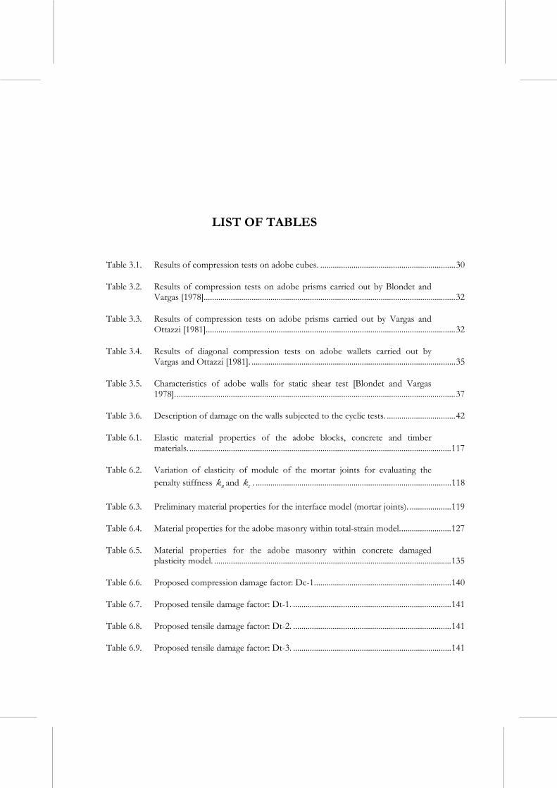
Table 3.1. Results of compression tests on adobe cubes. .................................................................30
Table 3.2. Results of compression tests on adobe prisms carried out by Blondet and Vargas [1978].........................................................................................................................32
Table 3.3. Results of compression tests on adobe prisms carried out by Vargas and Ottazzi [1981]........................................................................................................................32
Table 3.4. Results of diagonal compression tests on adobe wallets carried out by Vargas and Ottazzi [1981]. ..................................................................................................35
Table 3.5. Characteristics of adobe walls for static shear test [Blondet and Vargas 1978].......................................................................................................................................37
Table 3.6. Description of damage on the walls subjected to the cyclic tests. .................................42
Table 6.1. Elastic material properties of the adobe blocks, concrete and timber materials. ..............................................................................................................................117
Table 6.2. Variation of elasticity of module of the mortar joints for evaluating the penalty stiffness nk and sk . ..............................................................................................118
Table 6.3. Preliminary material properties for the interface model (mortar joints). ....................119
Table 6.4. Material properties for the adobe masonry within total-strain model.........................127
Table 6.5. Material properties for the adobe masonry within concrete damaged plasticity model. ..................................................................................................................135
Table 6.6. Proposed compression damage factor: Dc-1..................................................................140
Table 6.7. Proposed tensile damage factor: Dt-1. ............................................................................141
Table 6.8. Proposed tensile damage factor: Dt-2. ............................................................................141
Table 6.9. Proposed tensile damage factor: Dt-3. ............................................................................141
Sabino Nicola Tarque Ruiz
xxvi
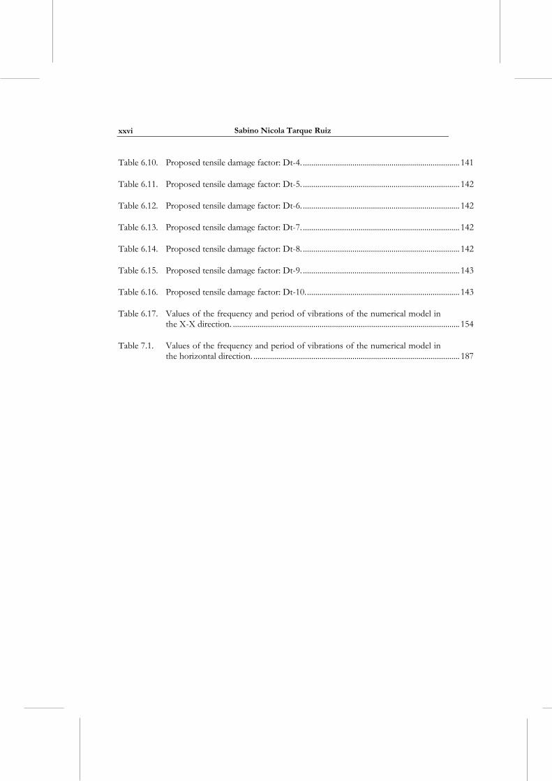
Table 6.10. Proposed tensile damage factor: Dt-4. ............................................................................ 141
Table 6.11. Proposed tensile damage factor: Dt-5. ............................................................................ 142
Table 6.12. Proposed tensile damage factor: Dt-6. ............................................................................ 142
Table 6.13. Proposed tensile damage factor: Dt-7. ............................................................................ 142
Table 6.14. Proposed tensile damage factor: Dt-8. ............................................................................ 142
Table 6.15. Proposed tensile damage factor: Dt-9. ............................................................................ 143
Table 6.16. Proposed tensile damage factor: Dt-10........................................................................... 143
Table 6.17. Values of the frequency and period of vibrations of the numerical model in the X-X direction. .............................................................................................................. 154
Table 7.1. Values of the frequency and period of vibrations of the numerical model in the horizontal direction. .................................................................................................... 187
1. INTRODUCTION
1.1 GENERAL
Adobe is a Spanish word derived from the Arabic atob, which literally means sun-dried brick, and it is one of the oldest and most widely used natural building materials, especially in developing countries (Latin America, Middle East, north and south of Africa, etc.) where there is also a moderate to high seismic hazard. The use of sun-dried blocks dates back to 8000 B.C. and till the last century was estimated that around 30% of the world’s population lives in earth-made construction [Houben and Guillard 1994]. Adobe and adobe construction have some attractive characteristics, such as low cost, local availability, self/owner-made or the need for only unskilled labour (hence the term “non-engineered constructions”), good thermal insulation and acoustic properties [Memari and Kauffman 2005].
Adobe buildings have high seismic vulnerability due to the low tension strength of the material, which ends in an undesirable combination of mechanical properties for these constructions, namely: 1) earthen structures are massive and thus attract large inertia forces; 2) they are weak and cannot resist these forces; and, 3) they are brittle and collapse without warning [Blondet et al. 2006]. The seismic capacity of an adobe house depends on the individual block mechanical characteristics, building location and design, and on the quality of the construction and maintenance [Dowling 2004]. Each time an earthquake occurs in a region with abundant earth-construction, enormous social and economical losses are recorded, as has been the case in El Salvador (2001), Iran (2003), Peru (1970, 1996, 2001 and 2007), Pakistan (2005), China (2008 and 2009).
Around the world only few universities and laboratories have been studied the seismic behaviour of adobe constructions (e.g. Pontificia Universidad Católica del Perú, University of Aveiro in Portugal, University of Basilicata in Italy, The Getty Conservation Institute in USA, Stanford University in USA, Institute of Earthquake Engineering and Engineering Seismology in Republic of Macedonia, Saitama University in Japan). The author of this thesis was involved into the dynamic experimental campaign for analyzing the seismic behaviour of unreinforced and reinforced adobe dwellings at the Pontificia Universidad Católica del Perú [Blondet et al. 2006] with partial support from the Getty Conservation Institute (GCI).
Sabino Nicola Tarque Ruíz
2
The tests for material characterization of adobe blocks as well as cyclic and dynamic tests reveal that the adobe mechanical properties (i.e. compression strength, elasticity modulus, shear strength, etc.) and the seismic performance of adobe constructions highly depend on the type of soil used for the production of units and mortar (i.e. Vargas et al. [2005], Yamin et al. [2004], Liberatore et al. [2006], Silveira et al. [2007]).
The analysis of the mechanical behaviour of adobe constructions still represents a true challenge. In this sense, researchers have been modelling the seismic behaviour of unreinforced masonry structures (URM), where adobe buildings can be included. However, little works for specific numerical modelling of adobe constructions (such as monuments or dwellings) has been done and the approach can focus to the micro-modelling of the individual components (bricks and mortar) or to the macro-modelling of masonry as a composite.
One of the major difficulties for numerical modelling of adobe constructions is the lack of information about material properties (especially the inelastic ones) and, in some cases, the geometric and structural complexity of the buildings. However, some calibration of the material properties and some simplifications for the geometry can be done (by using a finite element or discrete element method) in order to have good approximation of the seismic behaviour of adobe constructions, as presented in this work.
1.2 JUSTIFICATION
In some countries, especially those located in South-America and the Middle East, there exist many adobe constructions, from monuments until dwellings. The seismic behaviour of these buildings is not adequate. In order to reduce the inherent high seismic risk of these buildings, it is important to implement an adequate methodology to study their seismic behaviour through experimental and numerical modelling. Since dynamic tests are costly, a good alternative for analyzing the seismic vulnerability of adobe buildings -and therefore the justification of this work- is through numerical modelling.
1.3 ASSUMPTIONS
The main assumption of this research is that it is possible to generate numerical models to represent the dynamic behaviour of adobe buildings, serving as a tool for vulnerability assessment of constructions and risk analysis of sites.
Another assumption concerns the finite element approaches developed for the analysis of concrete and masonry panels; these models can be used for representing the behaviour of the adobe masonry, treated as an isotropic material.
Numerical modelling of the seismic behaviour of adobe buildings
3
1.4 OBJECTIVES
The general objective of this work is to calibrate the material properties of the adobe masonry for assessing the seismic vulnerability of adobe constructions through non-linear dynamic analyses.
The specific objectives of this research are:
1) To gather information about the material properties of adobe bricks, and pseudo-static and dynamic tests carried out on adobe constructions;
2) To better understand the seismic behaviour of adobe dwellings subjected to earthquakes;
3) To numerically represent the failure pattern and seismic capacity of cyclic and dynamic tests carried out on adobe masonry.
1.5 THESIS OUTLINE
The thesis is organized as follows: Chapter 2 presents a summary of the evolution of adobe construction in Peru, initiating from Caral city, which is considered the oldest American city funded around 3000 BC, until the present time. The poor geometrical configuration of vernacular adobe dwellings is discussed too, especially the ones located at the coastal sub-urban areas which typically host families with low income. Peru is a country with tradition in constructing with adobe. Nowadays, the total adobe construction represents about 43% of the total number of buildings. Based on a survey of damage carried out after the last big Peruvian earthquake (2007), the seismic behaviour of unreinforced and reinforced adobe dwellings is also discussed. Different materials for seismic reinforcement of adobe building are presented based on researches carried out mainly at the Pontificia Universidad Católica del Perú (PUCP).
The principal input data in any numerical analysis are the properties of the studied material, in this case the adobe masonry. Chapter 3 summarizes the experimental tests carried out at the Pontificia Universidad Católica del Perú, which started in the early 80’s with compression and diagonal tests on adobe masonry and shear tests on full adobe walls. Besides, the results of cyclic and dynamic tests carried out on adobe walls and adobe modules, respectively, are analyzed in terms of failure pattern and seismic capacity. These last tests were carried out in 2004 and 2005 with the participation of the theis’s author. The analyzed data from the static tests allows to compute the elasticity modulus, shear modulus, compression and tension strength of the adobe masonry; while the pseudo-static and dynamic results allow the calibration of the principal material properties (especially in the inelastic part) for matching the failure pattern of the numerical models developed in the following chapters.
Sabino Nicola Tarque Ruíz
4
The numerical analysis of unreinforced masonry structures (URM) has been studied by many authors and a summary of these analyses is presented in Chapter 4. Generally, the modelling analyses are based on a micro or macro modelling. The first assumes discontinuities between the masonry components (mortar and bricks), while the second assumes a distributed damage all over the masonry panel without distinction between mortar and bricks. In this thesis the finite element models used for analysis of cracking and damage on masonry and concrete panels are used for the evaluation of the seismic capacity of the adobe masonry.
Chapter 5 presents the theory of the finite element approaches for modelling the cracking and damage of concrete and masonry panels. These approaches are used in this thesis for the analysis of the adobe walls. Besides, a review of the theory of plasticity is presented with emphasis on the concepts of yield criterion, flow rule and softening/hardening law. As previously states, two main approaches exist for masonry analysis: the micro and macro modelling. For micro modelling a review of the composite model developed by Lourenço [1996] is presented. The finite element programme Midas FEA makes uses of this composite model. For macro-modelling a smeared crack model and a damaged plasticity model are discussed and used in this thesis with two programmes: Midas FEA and Abaqus (Standard and Explicit). At the end, constitutive laws for tension and compression behaviour of material such as adobe, masonry or concrete are described.
Taking advantage of the cyclic tests carried out by Blondet et al. [2005] and using the preliminary properties shown before, the material parameters both elastic and inelastic of the adobe masonry for loading and unloading are calibrated in Chapter 6. These material parameters -which are the input data for finite element models- should represent the failure pattern and seismic capacity of the tested adobe wall. Two finite element programmes are used here: Midas FEA and Abaqus/Standard, in both cases especial attention is given for the solution method and for the control parameters in order to avoid convergence problems. The first programme includes the composite model developed by Lourenço [1996] and a discrete analysis is performed. The adobe wall is also modelled using a smeared crack approach in Midas FEA and a concrete damaged plasticity model in Abaqus/Standard.
In Chapter 7 the dynamic analysis carried out by Blondet et al. [2006] on an adobe module is modelled using Abaqus/Standard and Abaqus/Explicit. The principal difference between these two methods is the way how the nodal accelerations, nodal velocities and nodal displacements are computed. The material properties used are the ones calibrated in Chapter 6. The experimental model was subjected to three levels of displacement records at the base, in this thesis just the second level is reproduced since it was related to the initiation of damage on the adobe walls. This chapter ends with the comparison

Numerical modelling of the seismic behaviour of adobe buildings
5
between the displacements records of the best numerical model and the experimental results.
Finally, Chapter 8 contains a summary of the work and explains the conclusions of the thesis. It also discusses and points to further research on modelling of adobe structures with different configurations but using the proposed material properties and modelling.

2. ADOBE HOUSES IN PERU
Adobe is one of the oldest materials used for civil and monumental constructions. It dates back to 8000 B.C. [Houben and Guillard 1994]. Archeological evidence shows entire cities built of raw earth, such as Jericho, history’s earliest city; Catal Hunyuk in Turkey; Harappa and Mohenjo-Daro in Pakistan; Akhlet-Aton in Egypt; Chan-Chan in Peru; Babylon in Iraq; Duheros near Cordoba in Spain and Khirokitia in Cyprus [Easton 2007]. The adobe brick is composed mainly of mud (clay, sand and silt), straw and water, and can be cast into a desired form. The straw is added to the bricks in order to reduce the cracking due to drying. The adobe constructions are relatively easy and fast to build; generally bricks are placed on top at each other with mud mortar.
Adobe was mostly used in areas with sparse water and vast open space but has been used effectively in cooler locations as well. When temperatures are low, adobe walls absorb and radiate heat throughout the house when the sun goes down. In the summer, the temperature in the house remains comfortable. In deserts, for example, where the climate is characterized by hot days and cool nights, the high thermal mass of adobe levels out the heat transfer through the wall to the living space.
In Peru, the adobe material is considered a traditional material. The majority of adobe dwellings can be found in the highlands cities, such as Cusco where more than 75% of the total buildings are made of adobe. Cusco is located at 3400 m altitude. However, unreinforced adobe constructions have a low seismic strength; they are considered brittle and use to collapse mainly by wall disconnection (out-of-plane actions). In this chapter, a brief review of the evolution of Peruvian adobe constructions and the analysis of the seismic behaviour of unreinforced and reinforced adobe houses is presented. Seismic reinforcement studied by professionals and researchers is also presented.
2.1 GENERALITIES
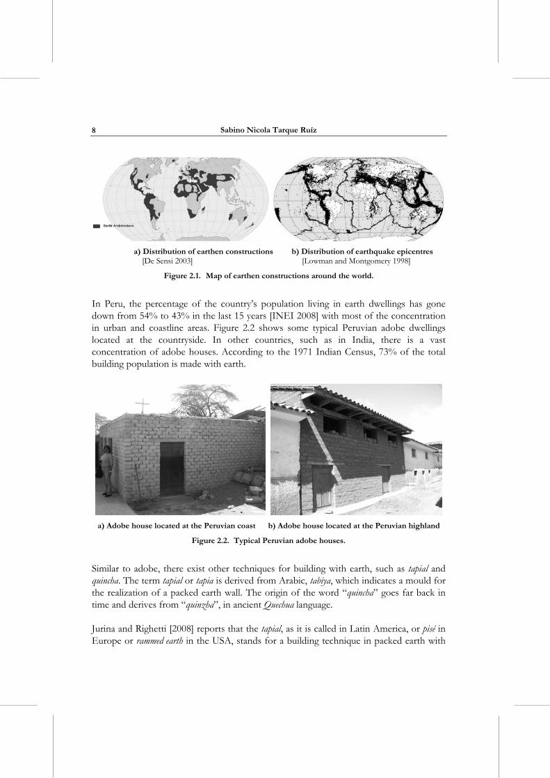
According to Houben and Guillard [1994] 30% of the world’s population lives in earth-made constructions, with approximately 50% of them located to developing countries. Adobe constructions are very common in some of the world’s most hazard-prone regions, such as Latin America, Africa, The Indian subcontinent and other parts of Asia, The Middle East and Southern Europe [Blondet et al. 2003]. Figure 2.1 compares the distribution of earthen constructions with the seismic hazard in the world.
Sabino Nicola Tarque Ruíz
8
a) Distribution of earthen constructions b) Distribution of earthquake epicentres [De Sensi 2003] [Lowman and Montgomery 1998]
Figure 2.1. Map of earthen constructions around the world.
In Peru, the percentage of the country’s population living in earth dwellings has gone down from 54% to 43% in the last 15 years [INEI 2008] with most of the concentration in urban and coastline areas. Figure 2.2 shows some typical Peruvian adobe dwellings located at the countryside. In other countries, such as in India, there is a vast concentration of adobe houses. According to the 1971 Indian Census, 73% of the total building population is made with earth.
a) Adobe house located at the Peruvian coast b) Adobe house located at the Peruvian highland
Figure 2.2. Typical Peruvian adobe houses.
Similar to adobe, there exist other techniques for building with earth, such as tapial and quincha. The term tapial or tapia is derived from Arabic, tabiya, which indicates a mould for the realization of a packed earth wall. The origin of the word “quincha” goes far back in time and derives from “quinzha”, in ancient Quechua language.
Jurina and Righetti [2008] reports that the tapial, as it is called in Latin America, or pisé in Europe or rammed earth in the USA, stands for a building technique in packed earth with
Numerical modelling of the seismic behaviour of adobe buildings
9
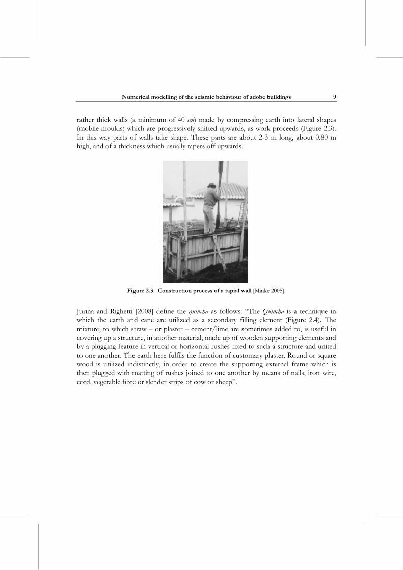
rather thick walls (a minimum of 40 cm) made by compressing earth into lateral shapes (mobile moulds) which are progressively shifted upwards, as work proceeds (Figure 2.3). In this way parts of walls take shape. These parts are about 2-3 m long, about 0.80 m high, and of a thickness which usually tapers off upwards.
Figure 2.3. Construction process of a tapial wall [Minke 2005].
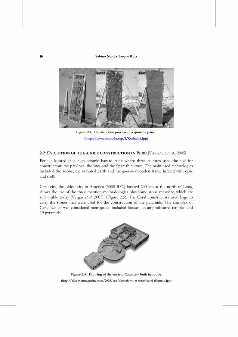
Jurina and Righetti [2008] define the quincha as follows: “The Quincha is a technique in which the earth and cane are utilized as a secondary filling element (Figure 2.4). The mixture, to which straw – or plaster – cement/lime are sometimes added to, is useful in covering up a structure, in another material, made up of wooden supporting elements and by a plugging feature in vertical or horizontal rushes fixed to such a structure and united to one another. The earth here fulfils the function of customary plaster. Round or square wood is utilized indistinctly, in order to create the supporting external frame which is then plugged with matting of rushes joined to one another by means of nails, iron wire, cord, vegetable fibre or slender strips of cow or sheep”.
Sabino Nicola Tarque Ruíz
10
Figure 2.4. Construction process of a quincha panel.
(http://www.soukala.org/i/Quincha.jpg)
2.2 EVOLUTION OF THE ADOBE CONSTRUCTION IN PERU [VARGAS ET AL. 2005]
Peru is located in a high seismic hazard zone where three cultures used the soil for construction: the pre-Inca, the Inca and the Spanish culture. The main used technologies included the adobe, the rammed earth and the quincha (wooden frame infilled with cane and soil).
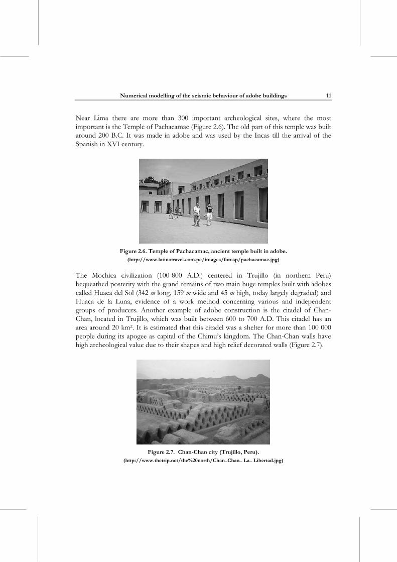
Caral city, the oldest city in America (3000 B.C.) located 200 km at the north of Lima, shows the use of the three mention methodologies plus some stone masonry, which are still visible today [Vargas et al. 2005], (Figure 2.5). The Caral constructors used bags to carry the stones that were used for the construction of the pyramids. The complex of Caral -which was considered metropolis- included houses, an amphitheatre, temples and 19 pyramids.
Figure 2.5. Drawing of the ancient Caral city built in adobe.
(http://discovermagazine.com/2005/sep/showdown-at-caral/caral-diagram.jpg)
Numerical modelling of the seismic behaviour of adobe buildings
11
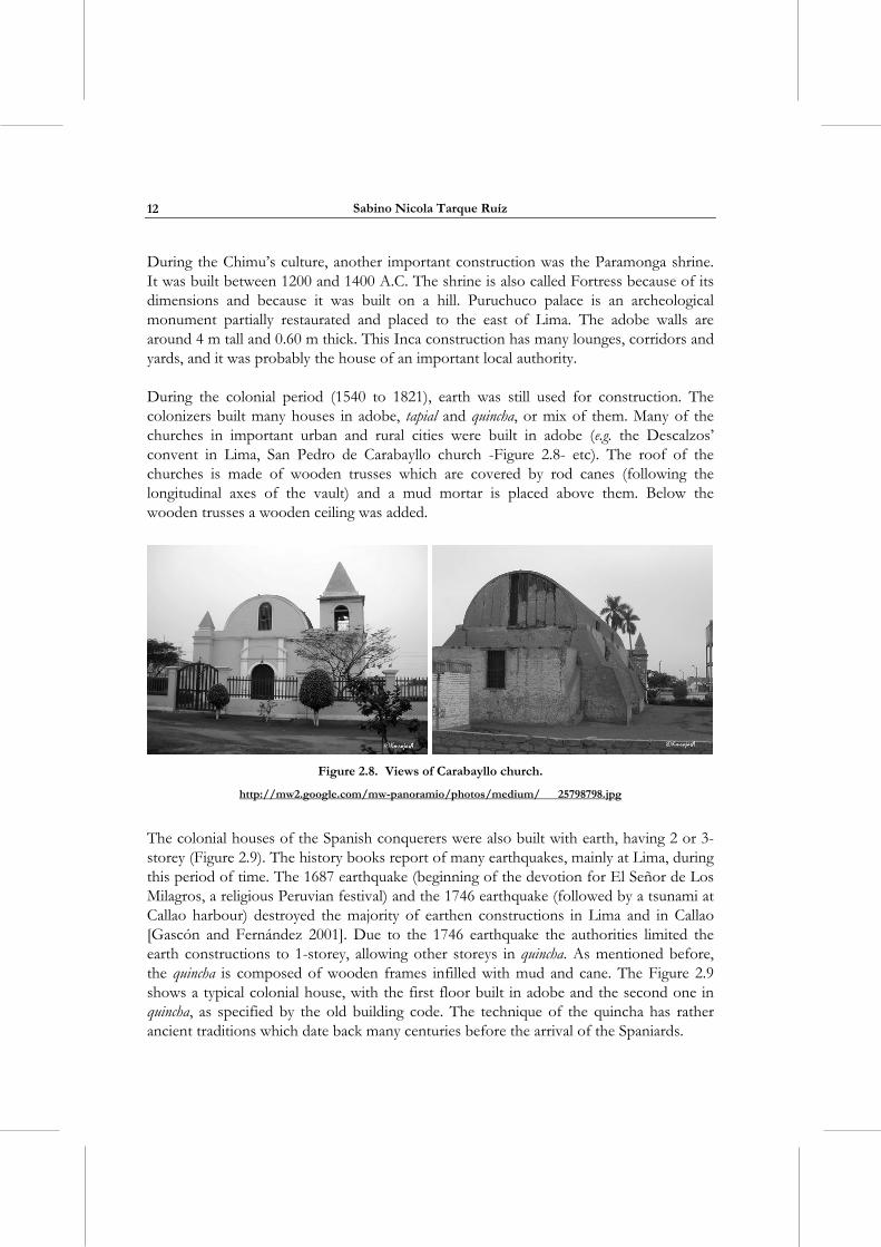
Near Lima there are more than 300 important archeological sites, where the most important is the Temple of Pachacamac (Figure 2.6). The old part of this temple was built around 200 B.C. It was made in adobe and was used by the Incas till the arrival of the Spanish in XVI century.
Figure 2.6. Temple of Pachacamac, ancient temple built in adobe.
(http://www.latinotravel.com.pe/images/fotosp/pachacamac.jpg)
The Mochica civilization (100-800 A.D.) centered in Trujillo (in northern Peru) bequeathed posterity with the grand remains of two main huge temples built with adobes called Huaca del Sol (342 m long, 159 m wide and 45 m high, today largely degraded) and Huaca de la Luna, evidence of a work method concerning various and independent groups of producers. Another example of adobe construction is the citadel of Chan-Chan, located in Trujillo, which was built between 600 to 700 A.D. This citadel has an area around 20 km2. It is estimated that this citadel was a shelter for more than 100 000 people during its apogee as capital of the Chimu’s kingdom. The Chan-Chan walls have high archeological value due to their shapes and high relief decorated walls (Figure 2.7).
Figure 2.7. Chan-Chan city (Trujillo, Peru).
(http://www.thetrip.net/the%20north/Chan_Chan_ La_ Libertad.jpg)
Sabino Nicola Tarque Ruíz
12
During the Chimu’s culture, another important construction was the Paramonga shrine. It was built between 1200 and 1400 A.C. The shrine is also called Fortress because of its dimensions and because it was built on a hill. Puruchuco palace is an archeological monument partially restaurated and placed to the east of Lima. The adobe walls are around 4 m tall and 0.60 m thick. This Inca construction has many lounges, corridors and yards, and it was probably the house of an important local authority.
During the colonial period (1540 to 1821), earth was still used for construction. The colonizers built many houses in adobe, tapial and quincha, or mix of them. Many of the churches in important urban and rural cities were built in adobe (e.g. the Descalzos’ convent in Lima, San Pedro de Carabayllo church -Figure 2.8- etc). The roof of the churches is made of wooden trusses which are covered by rod canes (following the longitudinal axes of the vault) and a mud mortar is placed above them. Below the wooden trusses a wooden ceiling was added.
Figure 2.8. Views of Carabayllo church.
http://mw2.google.com/mw-panoramio/photos/medium/ 25798798.jpg
The colonial houses of the Spanish conquerers were also built with earth, having 2 or 3-storey (Figure 2.9). The history books report of many earthquakes, mainly at Lima, during this period of time. The 1687 earthquake (beginning of the devotion for El Señor de Los Milagros, a religious Peruvian festival) and the 1746 earthquake (followed by a tsunami at Callao harbour) destroyed the majority of earthen constructions in Lima and in Callao [Gascón and Fernández 2001]. Due to the 1746 earthquake the authorities limited the earth constructions to 1-storey, allowing other storeys in quincha. As mentioned before, the quincha is composed of wooden frames infilled with mud and cane. The Figure 2.9 shows a typical colonial house, with the first floor built in adobe and the second one in quincha, as specified by the old building code. The technique of the quincha has rather ancient traditions which date back many centuries before the arrival of the Spaniards.
Numerical modelling of the seismic behaviour of adobe buildings
13
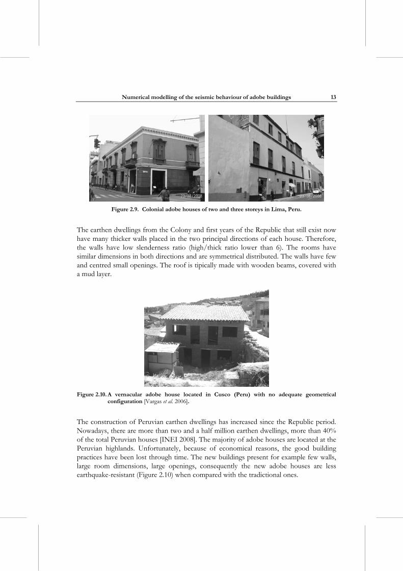
Figure 2.9. Colonial adobe houses of two and three storeys in Lima, Peru.
The earthen dwellings from the Colony and first years of the Republic that still exist now have many thicker walls placed in the two principal directions of each house. Therefore, the walls have low slenderness ratio (high/thick ratio lower than 6). The rooms have similar dimensions in both directions and are symmetrical distributed. The walls have few and centred small openings. The roof is tipically made with wooden beams, covered with a mud layer.
Figure 2.10. A vernacular adobe house located in Cusco (Peru) with no adequate geometrical
configuration [Vargas et al. 2006].
The construction of Peruvian earthen dwellings has increased since the Republic period. Nowadays, there are more than two and a half million earthen dwellings, more than 40% of the total Peruvian houses [INEI 2008]. The majority of adobe houses are located at the Peruvian highlands. Unfortunately, because of economical reasons, the good building practices have been lost through time. The new buildings present for example few walls, large room dimensions, large openings, consequently the new adobe houses are less earthquake-resistant (Figure 2.10) when compared with the tradictional ones.
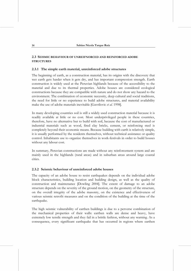
Sabino Nicola Tarque Ruíz
14
2.3 SEISMIC BEHAVIOUR OF UNREIFNORCED AND REINFORCED ADOBE
STRUCTURES
2.3.1 The simple earth material, unreinforced adobe structures
The beginning of earth, as a construction material, has its origins with the discovery that wet earth gets harder when it gets dry, and has important compression strength. Earth construction is widely used at the Peruvian highlands because of the accessibility to the material and due to its thermal properties. Adobe houses are considered ecological constructions because they are compatible with nature and do not show any hazard to the environment. The combination of economic necessity, deep cultural and social traditions, the need for little or no experience to build adobe structures, and material availability make the use of adobe materials inevitable [Gavrilovic et al. 1998].
In many developing countries soil is still a widely used construction material because it is readily available at little or no cost. Most underprivileged people in these countries, therefore, have no alternative but to build with soil, because the cost of manufactured or industrial materials such as wood, fired clay bricks, cement, or reinforcing steel is completely beyond their economic means. Because building with earth is relatively simple, it is usually performed by the residents themselves, without technical assistance or quality control. Inhabitants use to organize themselves in work-festivals in order to build houses without any labour cost.
In summary, Peruvian constructions are made without any reinforcement system and are mainly used in the highlands (rural areas) and in suburban areas around large coastal cities.
2.3.2 Seismic behaviour of unreinforced adobe houses
The capacity of an adobe house to resist earthquakes depends on the individual adobe block characteristics, building location and building design, as well as the quality of construction and maintenance [Dowling 2004]. The extent of damage to an adobe structure depends on the severity of the ground motion, on the geometry of the structure, on the overall integrity of the adobe masonry, on the existence and effectiveness of various seismic retrofit measures and on the condition of the building at the time of the earthquake.
The high seismic vulnerability of earthen buildings is due to a perverse combination of the mechanical properties of their walls: earthen walls are dense and heavy, have extremely low tensile strength and they fail in a brittle fashion, without any warning. As a consequence, every significant earthquake that has occurred in regions where earthen
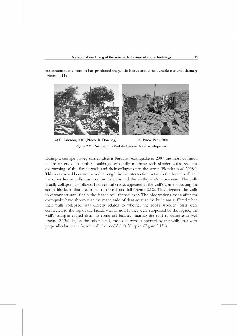
Numerical modelling of the seismic behaviour of adobe buildings
15
construction is common has produced tragic life losses and considerable material damage (Figure 2.11).
a) El Salvador, 2001 (Photo: D. Dowling) b) Pisco, Peru, 2007
Figure 2.11. Destruction of adobe houses due to earthquakes.
During a damage survey carried after a Peruvian earthquake in 2007 the most common failure observed in earthen buildings, especially in those with slender walls, was the overturning of the façade walls and their collapse onto the street [Blondet et al. 2008a]. This was caused because the wall strength in the intersection between the façade wall and the other house walls was too low to withstand the earthquake’s movement. The walls usually collapsed as follows: first vertical cracks appeared at the wall’s corners causing the adobe blocks in that area to start to break and fall (Figure 2.12). This triggered the walls to disconnect until finally the façade wall flipped over. The observations made after the earthquake have shown that the magnitude of damage that the buildings suffered when their walls collapsed, was directly related to whether the roof’s wooden joists were connected to the top of the façade wall or not. If they were supported by the façade, the wall’s collapse caused them to come off balance, causing the roof to collapse as well (Figure 2.13a). If, on the other hand, the joists were supported by the walls that were perpendicular to the façade wall, the roof didn’t fall apart (Figure 2.13b).
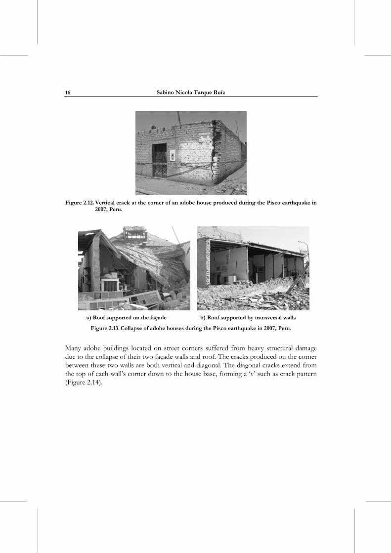
Sabino Nicola Tarque Ruíz
16
Figure 2.12. Vertical crack at the corner of an adobe house produced during the Pisco earthquake in
2007, Peru.
a) Roof supported on the façade b) Roof supported by transversal walls
Figure 2.13. Collapse of adobe houses during the Pisco earthquake in 2007, Peru.
Many adobe buildings located on street corners suffered from heavy structural damage due to the collapse of their two façade walls and roof. The cracks produced on the corner between these two walls are both vertical and diagonal. The diagonal cracks extend from the top of each wall’s corner down to the house base, forming a ‘v’ such as crack pattern (Figure 2.14).
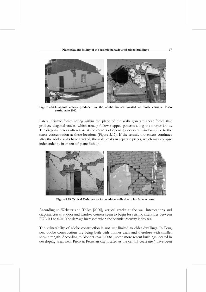
Numerical modelling of the seismic behaviour of adobe buildings
17
Figure 2.14. Diagonal cracks produced in the adobe houses located at block corners, Pisco
earthquake 2007.
Lateral seismic forces acting within the plane of the walls generate shear forces that produce diagonal cracks, which usually follow stepped patterns along the mortar joints. The diagonal cracks often start at the corners of opening doors and windows, due to the stress concentration at these locations (Figure 2.15). If the seismic movement continues after the adobe walls have cracked, the wall breaks in separate pieces, which may collapse independently in an out-of-plane fashion.
Figure 2.15. Typical X-shape cracks on adobe walls due to in-plane actions.
According to Webster and Tolles [2000], vertical cracks at the wall intersections and diagonal cracks at door and window corners seem to begin for seismic intensities between PGA 0.1 to 0.2g. The damage increases when the seismic intensity increases.
The vulnerability of adobe construction is not just limited to older dwellings. In Peru, new adobe constructions are being built with thinner walls and therefore with smaller shear strength. According to Blondet et al. [2008a], some more recent buildings located in developing areas near Pisco (a Peruvian city located at the central coast area) have been
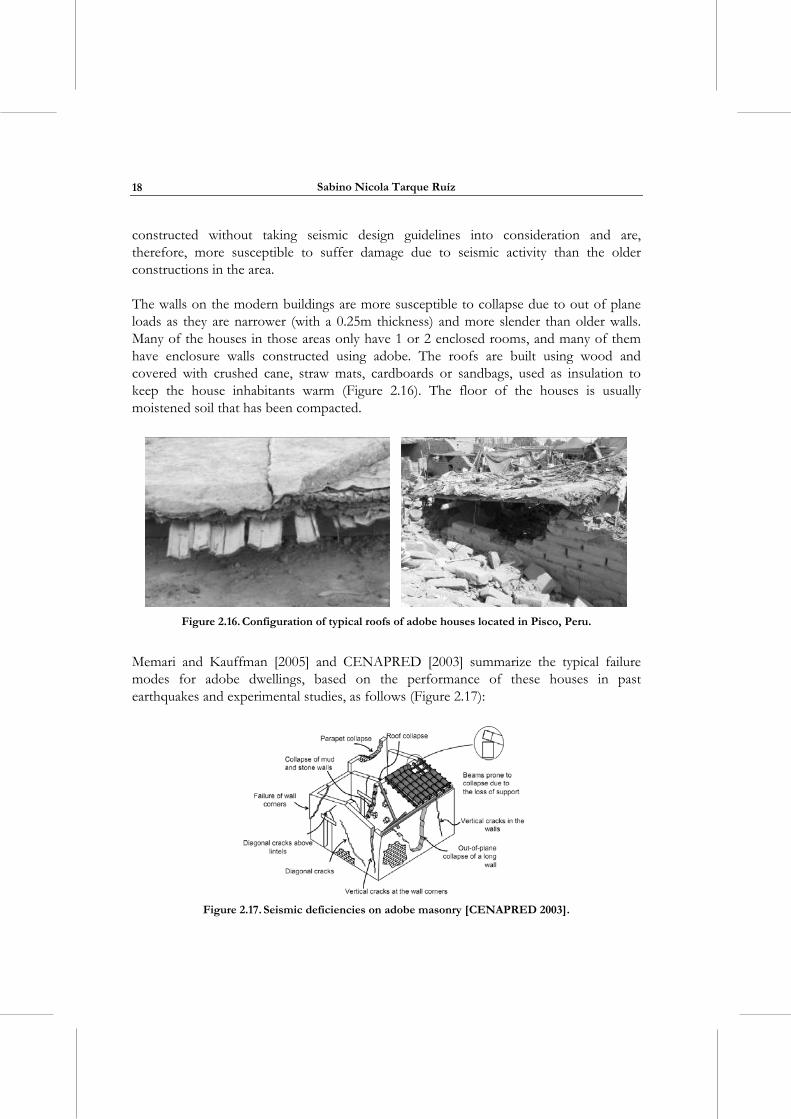
Sabino Nicola Tarque Ruíz
18
constructed without taking seismic design guidelines into consideration and are, therefore, more susceptible to suffer damage due to seismic activity than the older constructions in the area.
The walls on the modern buildings are more susceptible to collapse due to out of plane loads as they are narrower (with a 0.25m thickness) and more slender than older walls. Many of the houses in those areas only have 1 or 2 enclosed rooms, and many of them have enclosure walls constructed using adobe. The roofs are built using wood and covered with crushed cane, straw mats, cardboards or sandbags, used as insulation to keep the house inhabitants warm (Figure 2.16). The floor of the houses is usually moistened soil that has been compacted.
Figure 2.16. Configuration of typical roofs of adobe houses located in Pisco, Peru.
Memari and Kauffman [2005] and CENAPRED [2003] summarize the typical failure modes for adobe dwellings, based on the performance of these houses in past earthquakes and experimental studies, as follows (Figure 2.17):
Figure 2.17. Seismic deficiencies on adobe masonry [CENAPRED 2003].
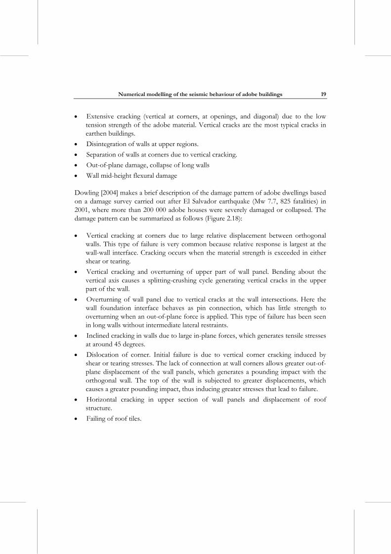
Numerical modelling of the seismic behaviour of adobe buildings
19
Extensive cracking (vertical at corners, at openings, and diagonal) due to the low tension strength of the adobe material. Vertical cracks are the most typical cracks in earthen buildings.
Disintegration of walls at upper regions.
Separation of walls at corners due to vertical cracking.
Out-of-plane damage, collapse of long walls
Wall mid-height flexural damage
Dowling [2004] makes a brief description of the damage pattern of adobe dwellings based on a damage survey carried out after El Salvador earthquake (Mw 7.7, 825 fatalities) in 2001, where more than 200 000 adobe houses were severely damaged or collapsed. The damage pattern can be summarized as follows (Figure 2.18):
Vertical cracking at corners due to large relative displacement between orthogonal walls. This type of failure is very common because relative response is largest at the wall-wall interface. Cracking occurs when the material strength is exceeded in either shear or tearing.
Vertical cracking and overturning of upper part of wall panel. Bending about the vertical axis causes a splitting-crushing cycle generating vertical cracks in the upper part of the wall.
Overturning of wall panel due to vertical cracks at the wall intersections. Here the wall foundation interface behaves as pin connection, which has little strength to overturning when an out-of-plane force is applied. This type of failure has been seen in long walls without intermediate lateral restraints.
Inclined cracking in walls due to large in-plane forces, which generates tensile stresses at around 45 degrees.
Dislocation of corner. Initial failure is due to vertical corner cracking induced by shear or tearing stresses. The lack of connection at wall corners allows greater out-of-plane displacement of the wall panels, which generates a pounding impact with the orthogonal wall. The top of the wall is subjected to greater displacements, which causes a greater pounding impact, thus inducing greater stresses that lead to failure.
Horizontal cracking in upper section of wall panels and displacement of roof structure.
Failing of roof tiles.
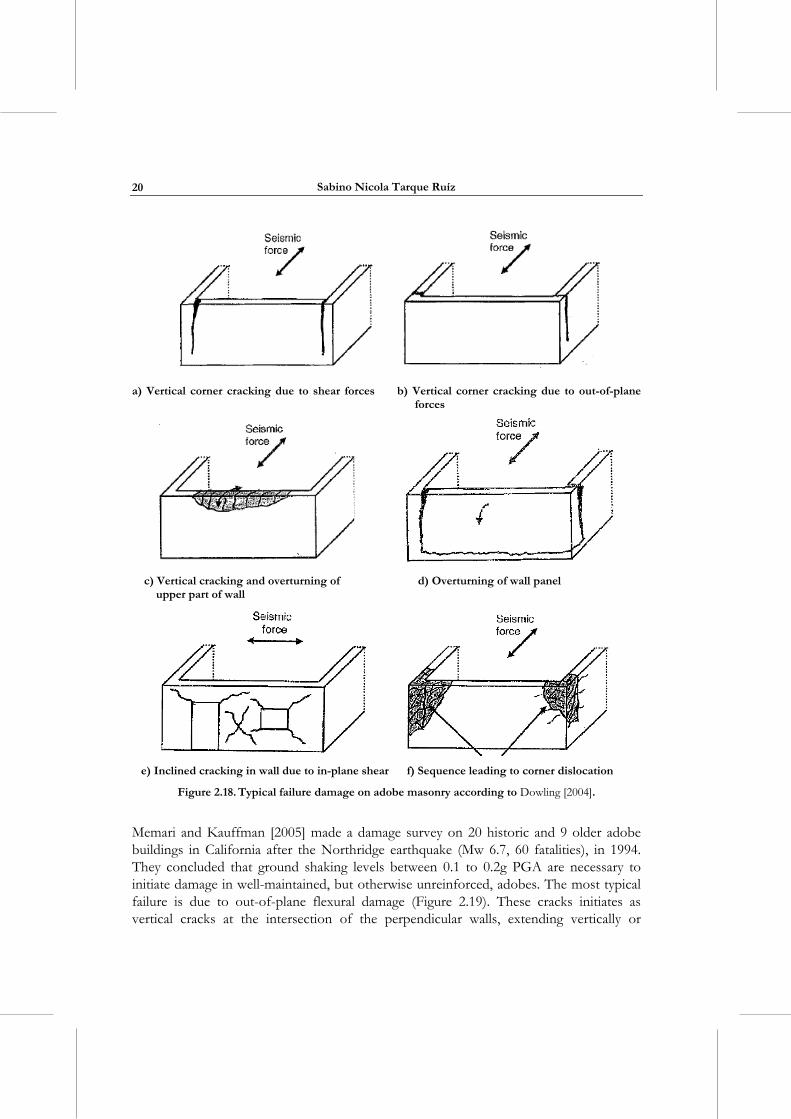
Sabino Nicola Tarque Ruíz
20
a) Vertical corner cracking due to shear forces b) Vertical corner cracking due to out-of-plane
forces
c) Vertical cracking and overturning of d) Overturning of wall panel upper part of wall
e) Inclined cracking in wall due to in-plane shear f) Sequence leading to corner dislocation
Figure 2.18. Typical failure damage on adobe masonry according to Dowling [2004].
Memari and Kauffman [2005] made a damage survey on 20 historic and 9 older adobe buildings in California after the Northridge earthquake (Mw 6.7, 60 fatalities), in 1994. They concluded that ground shaking levels between 0.1 to 0.2g PGA are necessary to initiate damage in well-maintained, but otherwise unreinforced, adobes. The most typical failure is due to out-of-plane flexural damage (Figure 2.19). These cracks initiates as vertical cracks at the intersection of the perpendicular walls, extending vertically or
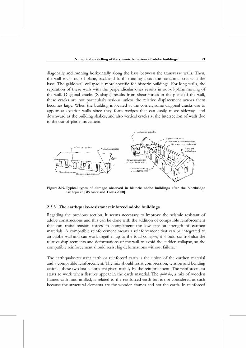
Numerical modelling of the seismic behaviour of adobe buildings
21
diagonally and running horizontally along the base between the transverse walls. Then, the wall rocks out-of-plane, back and forth, rotating about the horizontal cracks at the base. The gable-wall collapse is more specific for historic buildings. For long walls, the separation of these walls with the perpendicular ones results in out-of-plane moving of the wall. Diagonal cracks (X-shape) results from shear forces in the plane of the wall, these cracks are not particularly serious unless the relative displacement across them becomes large. When the building is located at the corner, some diagonal cracks use to appear at exterior walls since they form wedges that can easily move sideways and downward as the building shakes, and also vertical cracks at the intersection of walls due to the out-of-plane movement.
Figure 2.19. Typical types of damage observed in historic adobe buildings after the Northridge
earthquake [Webster and Tolles 2000].
2.3.3 The earthquake-resistant reinforced adobe buildings
Regading the previous section, it seems necessary to improve the seismic resistant of adobe constructions and this can be done with the addition of compatible reinforcement that can resist tension forces to complement the low tension strength of earthen materials. A compatible reinforcement means a reinforcement that can be integrated to an adobe wall and can work together up to the total collapse; it should control also the relative displacements and deformations of the wall to avoid the sudden collapse, so the compatible reinforcement should resist big deformations without failure.
The earthquake-resistant earth or reinforced earth is the union of the earthen material and a compatible reinforcement. The mix should resist compression, tension and bending actions, these two last actions are given mainly by the reinforcement. The reinforcement starts to work when fissures appear in the earth material. The quincha, a mix of wooden frames with mud infilled, is related to the reinforced earth but is not considered as such because the structural elements are the wooden frames and not the earth. In reinforced
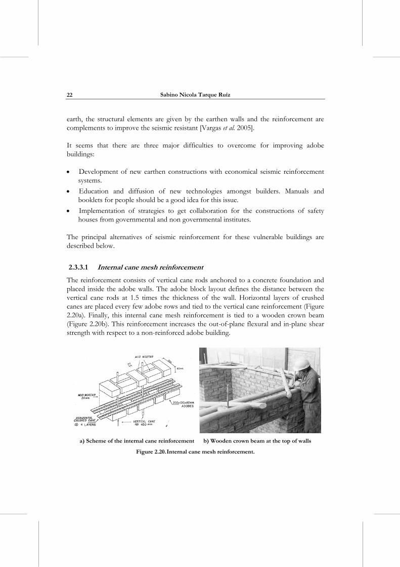
Sabino Nicola Tarque Ruíz
22
earth, the structural elements are given by the earthen walls and the reinforcement are complements to improve the seismic resistant [Vargas et al. 2005].
It seems that there are three major difficulties to overcome for improving adobe buildings:
Development of new earthen constructions with economical seismic reinforcement systems.
Education and diffusion of new technologies amongst builders. Manuals and booklets for people should be a good idea for this issue.
Implementation of strategies to get collaboration for the constructions of safety houses from governmental and non governmental institutes.
The principal alternatives of seismic reinforcement for these vulnerable buildings are described below.
2.3.3.1 Internal cane mesh reinforcement
The reinforcement consists of vertical cane rods anchored to a concrete foundation and placed inside the adobe walls. The adobe block layout defines the distance between the vertical cane rods at 1.5 times the thickness of the wall. Horizontal layers of crushed canes are placed every few adobe rows and tied to the vertical cane reinforcement (Figure 2.20a). Finally, this internal cane mesh reinforcement is tied to a wooden crown beam (Figure 2.20b). This reinforcement increases the out-of-plane flexural and in-plane shear strength with respect to a non-reinforced adobe building.
a) Scheme of the internal cane reinforcement b) Wooden crown beam at the top of walls
Figure 2.20. Internal cane mesh reinforcement.
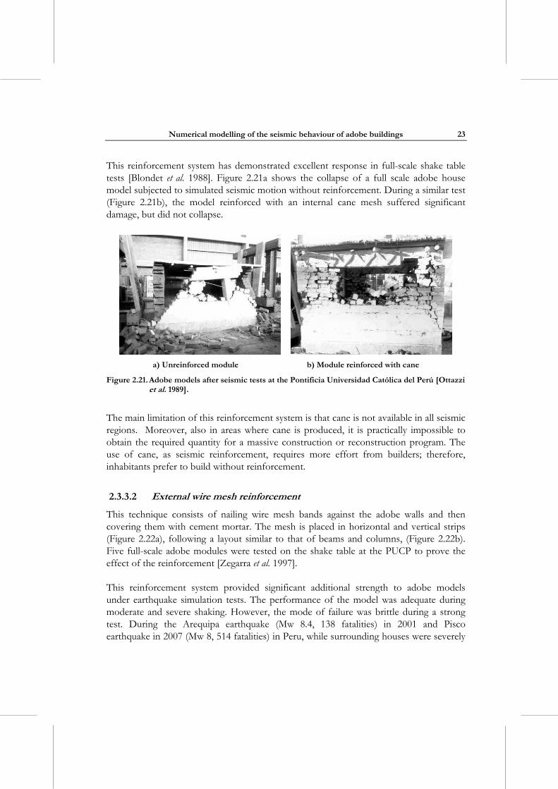
Numerical modelling of the seismic behaviour of adobe buildings
23
This reinforcement system has demonstrated excellent response in full-scale shake table tests [Blondet et al. 1988]. Figure 2.21a shows the collapse of a full scale adobe house model subjected to simulated seismic motion without reinforcement. During a similar test (Figure 2.21b), the model reinforced with an internal cane mesh suffered significant damage, but did not collapse.
a) Unreinforced module b) Module reinforced with cane
Figure 2.21. Adobe models after seismic tests at the Pontificia Universidad Católica del Perú [Ottazzi et al. 1989].
The main limitation of this reinforcement system is that cane is not available in all seismic regions. Moreover, also in areas where cane is produced, it is practically impossible to obtain the required quantity for a massive construction or reconstruction program. The use of cane, as seismic reinforcement, requires more effort from builders; therefore, inhabitants prefer to build without reinforcement.
2.3.3.2 External wire mesh reinforcement
This technique consists of nailing wire mesh bands against the adobe walls and then covering them with cement mortar. The mesh is placed in horizontal and vertical strips (Figure 2.22a), following a layout similar to that of beams and columns, (Figure 2.22b). Five full-scale adobe modules were tested on the shake table at the PUCP to prove the effect of the reinforcement [Zegarra et al. 1997].
This reinforcement system provided significant additional strength to adobe models under earthquake simulation tests. The performance of the model was adequate during moderate and severe shaking. However, the mode of failure was brittle during a strong test. During the Arequipa earthquake (Mw 8.4, 138 fatalities) in 2001 and Pisco earthquake in 2007 (Mw 8, 514 fatalities) in Peru, while surrounding houses were severely
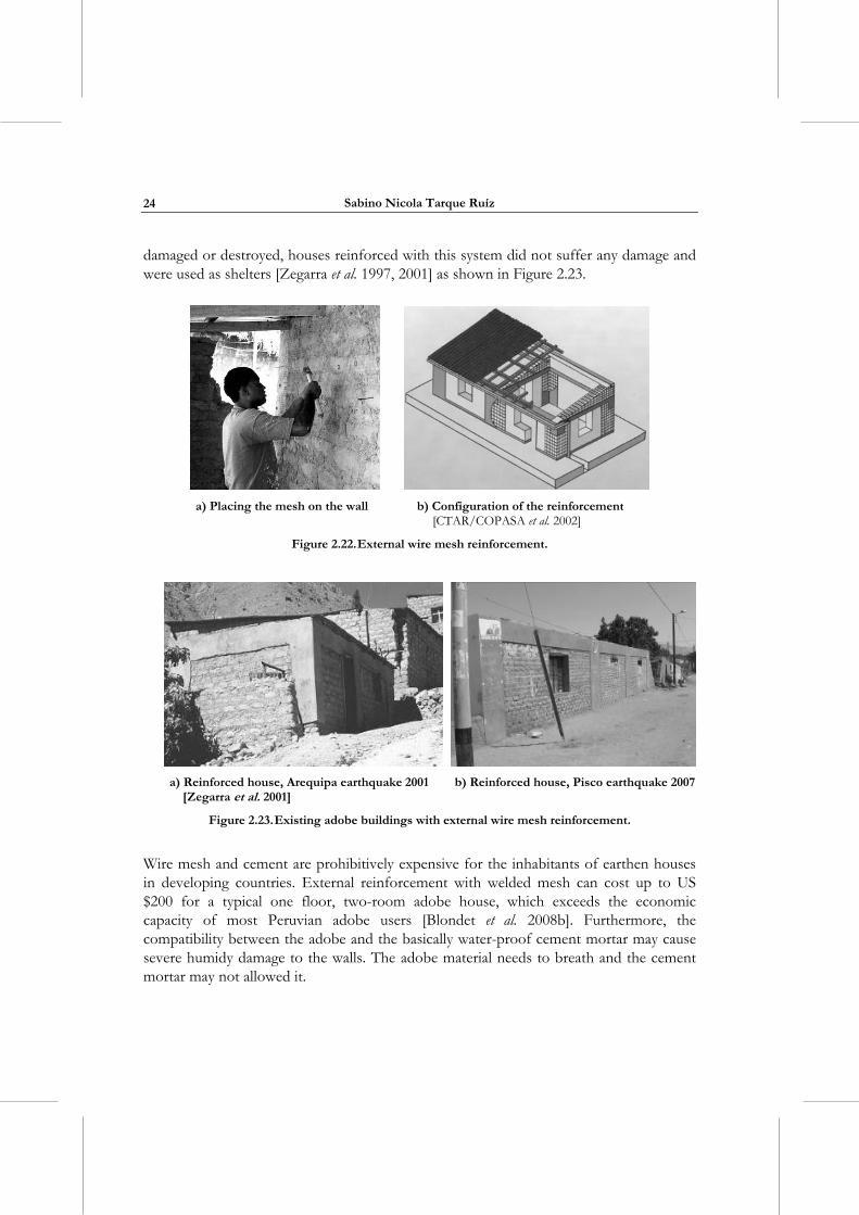
Sabino Nicola Tarque Ruíz
24
damaged or destroyed, houses reinforced with this system did not suffer any damage and were used as shelters [Zegarra et al. 1997, 2001] as shown in Figure 2.23.
a) Placing the mesh on the wall b) Configuration of the reinforcement
[CTAR/COPASA et al. 2002]
Figure 2.22. External wire mesh reinforcement.
a) Reinforced house, Arequipa earthquake 2001 b) Reinforced house, Pisco earthquake 2007 [Zegarra et al. 2001]
Figure 2.23. Existing adobe buildings with external wire mesh reinforcement.
Wire mesh and cement are prohibitively expensive for the inhabitants of earthen houses in developing countries. External reinforcement with welded mesh can cost up to US $200 for a typical one floor, two-room adobe house, which exceeds the economic capacity of most Peruvian adobe users [Blondet et al. 2008b]. Furthermore, the compatibility between the adobe and the basically water-proof cement mortar may cause severe humidy damage to the walls. The adobe material needs to breath and the cement mortar may not allowed it.
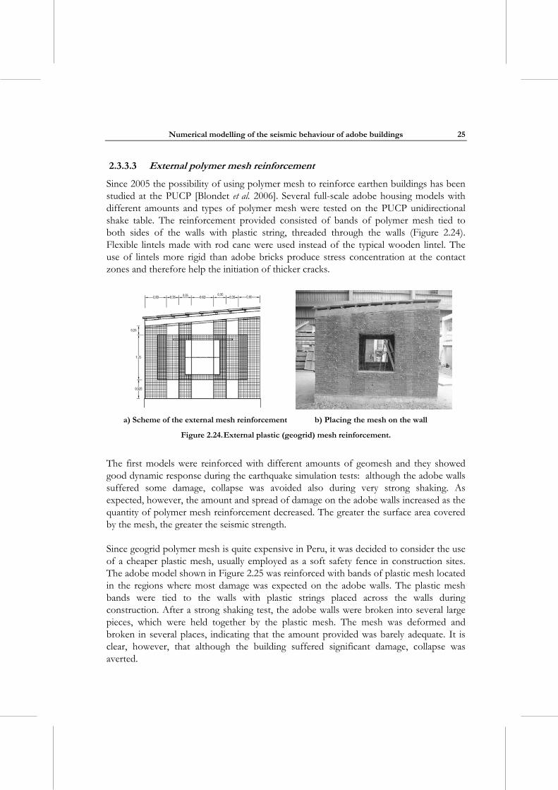
Numerical modelling of the seismic behaviour of adobe buildings
25
2.3.3.3 External polymer mesh reinforcement
Since 2005 the possibility of using polymer mesh to reinforce earthen buildings has been studied at the PUCP [Blondet et al. 2006]. Several full-scale adobe housing models with different amounts and types of polymer mesh were tested on the PUCP unidirectional shake table. The reinforcement provided consisted of bands of polymer mesh tied to both sides of the walls with plastic string, threaded through the walls (Figure 2.24). Flexible lintels made with rod cane were used instead of the typical wooden lintel. The use of lintels more rigid than adobe bricks produce stress concentration at the contact zones and therefore help the initiation of thicker cracks.
a) Scheme of the external mesh reinforcement b) Placing the mesh on the wall
Figure 2.24. External plastic (geogrid) mesh reinforcement.
The first models were reinforced with different amounts of geomesh and they showed good dynamic response during the earthquake simulation tests: although the adobe walls suffered some damage, collapse was avoided also during very strong shaking. As expected, however, the amount and spread of damage on the adobe walls increased as the quantity of polymer mesh reinforcement decreased. The greater the surface area covered by the mesh, the greater the seismic strength.
Since geogrid polymer mesh is quite expensive in Peru, it was decided to consider the use of a cheaper plastic mesh, usually employed as a soft safety fence in construction sites. The adobe model shown in Figure 2.25 was reinforced with bands of plastic mesh located in the regions where most damage was expected on the adobe walls. The plastic mesh bands were tied to the walls with plastic strings placed across the walls during construction. After a strong shaking test, the adobe walls were broken into several large pieces, which were held together by the plastic mesh. The mesh was deformed and broken in several places, indicating that the amount provided was barely adequate. It is clear, however, that although the building suffered significant damage, collapse was averted.
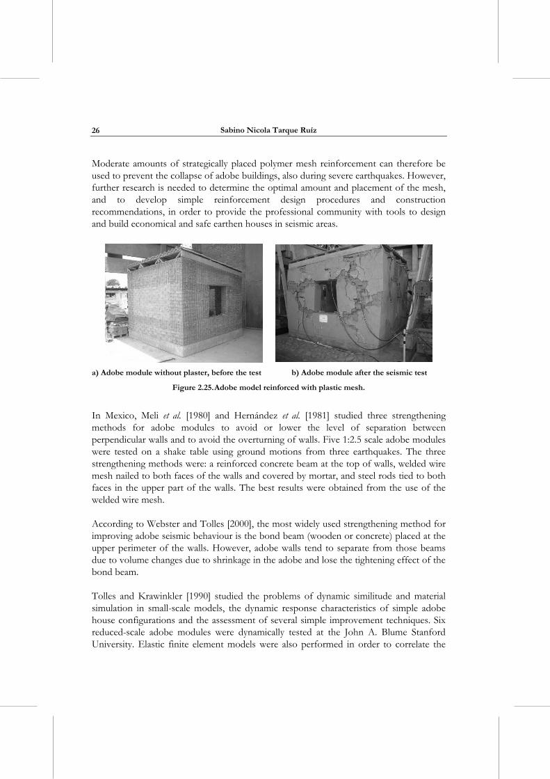
Sabino Nicola Tarque Ruíz
26
Moderate amounts of strategically placed polymer mesh reinforcement can therefore be used to prevent the collapse of adobe buildings, also during severe earthquakes. However, further research is needed to determine the optimal amount and placement of the mesh, and to develop simple reinforcement design procedures and construction recommendations, in order to provide the professional community with tools to design and build economical and safe earthen houses in seismic areas.
a) Adobe module without plaster, before the test b) Adobe module after the seismic test
Figure 2.25. Adobe model reinforced with plastic mesh.
In Mexico, Meli et al. [1980] and Hernández et al. [1981] studied three strengthening methods for adobe modules to avoid or lower the level of separation between perpendicular walls and to avoid the overturning of walls. Five 1:2.5 scale adobe modules were tested on a shake table using ground motions from three earthquakes. The three strengthening methods were: a reinforced concrete beam at the top of walls, welded wire mesh nailed to both faces of the walls and covered by mortar, and steel rods tied to both faces in the upper part of the walls. The best results were obtained from the use of the welded wire mesh.
According to Webster and Tolles [2000], the most widely used strengthening method for improving adobe seismic behaviour is the bond beam (wooden or concrete) placed at the upper perimeter of the walls. However, adobe walls tend to separate from those beams due to volume changes due to shrinkage in the adobe and lose the tightening effect of the bond beam.
Tolles and Krawinkler [1990] studied the problems of dynamic similitude and material simulation in small-scale models, the dynamic response characteristics of simple adobe house configurations and the assessment of several simple improvement techniques. Six reduced-scale adobe modules were dynamically tested at the John A. Blume Stanford University. Elastic finite element models were also performed in order to correlate the
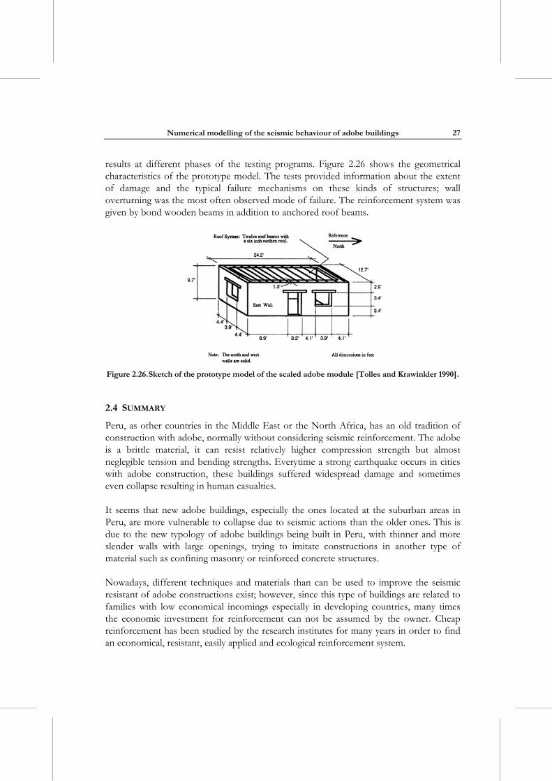
Numerical modelling of the seismic behaviour of adobe buildings
27
results at different phases of the testing programs. Figure 2.26 shows the geometrical characteristics of the prototype model. The tests provided information about the extent of damage and the typical failure mechanisms on these kinds of structures; wall overturning was the most often observed mode of failure. The reinforcement system was given by bond wooden beams in addition to anchored roof beams.
Figure 2.26. Sketch of the prototype model of the scaled adobe module [Tolles and Krawinkler 1990].
2.4 SUMMARY
Peru, as other countries in the Middle East or the North Africa, has an old tradition of construction with adobe, normally without considering seismic reinforcement. The adobe is a brittle material, it can resist relatively higher compression strength but almost neglegible tension and bending strengths. Everytime a strong earthquake occurs in cities with adobe construction, these buildings suffered widespread damage and sometimes even collapse resulting in human casualties.
It seems that new adobe buildings, especially the ones located at the suburban areas in Peru, are more vulnerable to collapse due to seismic actions than the older ones. This is due to the new typology of adobe buildings being built in Peru, with thinner and more slender walls with large openings, trying to imitate constructions in another type of material such as confining masonry or reinforced concrete structures.
Nowadays, different techniques and materials than can be used to improve the seismic resistant of adobe constructions exist; however, since this type of buildings are related to families with low economical incomings especially in developing countries, many times the economic investment for reinforcement can not be assumed by the owner. Cheap reinforcement has been studied by the research institutes for many years in order to find an economical, resistant, easily applied and ecological reinforcement system.
Sabino Nicola Tarque Ruíz
28
In this chapter, the inclusion of a minimum reinforcement (e.g. wooden crown beam, internal cane mesh, wire welded mesh or plastic mesh) into an adobe building is discussed and it is shown that it improves the seismic performance of adobe structures; therefore, avoiding casualties.
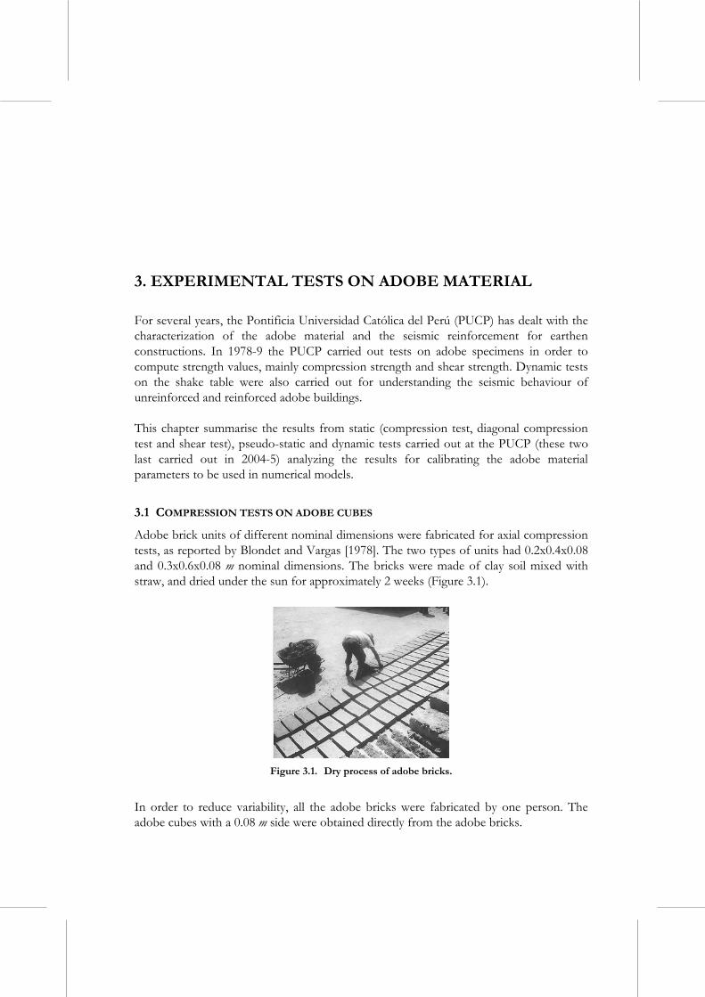
3. EXPERIMENTAL TESTS ON ADOBE MATERIAL
For several years, the Pontificia Universidad Católica del Perú (PUCP) has dealt with the characterization of the adobe material and the seismic reinforcement for earthen constructions. In 1978-9 the PUCP carried out tests on adobe specimens in order to compute strength values, mainly compression strength and shear strength. Dynamic tests on the shake table were also carried out for understanding the seismic behaviour of unreinforced and reinforced adobe buildings.
This chapter summarise the results from static (compression test, diagonal compression test and shear test), pseudo-static and dynamic tests carried out at the PUCP (these two last carried out in 2004-5) analyzing the results for calibrating the adobe material parameters to be used in numerical models.
3.1 COMPRESSION TESTS ON ADOBE CUBES
Adobe brick units of different nominal dimensions were fabricated for axial compression tests, as reported by Blondet and Vargas [1978]. The two types of units had 0.2x0.4x0.08 and 0.3x0.6x0.08 m nominal dimensions. The bricks were made of clay soil mixed with straw, and dried under the sun for approximately 2 weeks (Figure 3.1).
Figure 3.1. Dry process of adobe bricks.
In order to reduce variability, all the adobe bricks were fabricated by one person. The adobe cubes with a 0.08 m side were obtained directly from the adobe bricks.
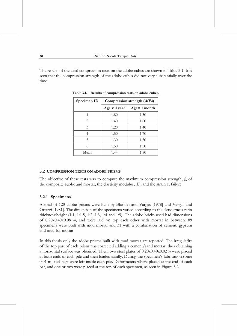
Sabino Nicola Tarque Ruíz
30
The results of the axial compression tests on the adobe cubes are shown in Table 3.1. It is seen that the compression strength of the adobe cubes did not vary substantially over the time.
Table 3.1. Results of compression tests on adobe cubes.
Compression strength (MPa) Specimen ID
Age > 1 year Age= 1 month
1 1.80 1.30
2 1.40 1.60
3 1.20 1.40
4 1.50 1.70
5 1.30 1.50
6 1.50 1.50
Mean 1.44 1.50
3.2 COMPRESSION TESTS ON ADOBE PRISMS
The objective of these tests was to compute the maximum compression strength, fc, of the composite adobe and mortar, the elasticity modulus, E , and the strain at failure.
3.2.1 Specimens
A total of 120 adobe prisms were built by Blondet and Vargas [1978] and Vargas and Ottazzi [1981]. The dimension of the specimens varied according to the slenderness ratio thickness:height (1:1, 1:1.5, 1:2, 1:3, 1:4 and 1:5). The adobe bricks used had dimensions of 0.20x0.40x0.08 m, and were laid on top each other with mortar in between: 89 specimens were built with mud mortar and 31 with a combination of cement, gypsum and mud for mortar.
In this thesis only the adobe prisms built with mud mortar are reported. The irregularity of the top part of each prism was corrected adding a cement/sand mortar, thus obtaining a horizontal surface was obtained. Then, two steel plates of 0.20x0.40x0.02 m were placed at both ends of each pile and then loaded axially. During the specimen’s fabrication some 0.01 m steel bars were left inside each pile. Deformeters where placed at the end of each bar, and one or two were placed at the top of each specimen, as seen in Figure 3.2.
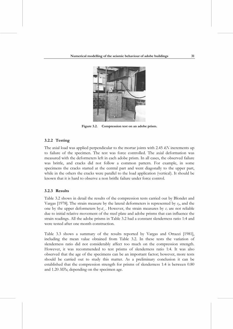
Numerical modelling of the seismic behaviour of adobe buildings
31
Figure 3.2. Compression test on an adobe prism.
3.2.2 Testing
The axial load was applied perpendicular to the mortar joints with 2.45 kN increments up to failure of the specimen. The test was force controlled. The axial deformation was measured with the deformeters left in each adobe prism. In all cases, the observed failure was brittle, and cracks did not follow a common pattern. For example, in some specimens the cracks started at the central part and went diagonally to the upper part, while in the others the cracks were parallel to the load application (vertical). It should be known that it is hard to observe a non britlle failure under force control.
3.2.3 Results
Table 3.2 shows in detail the results of the compression tests carried out by Blondet and Vargas [1978]. The strain measure by the lateral deformeters is represented by εp, and the one by the upper deformeters by s . However, the strain measures by εs are not reliable due to initial relative movement of the steel plate and adobe prisms that can influence the strain readings. All the adobe prisms in Table 3.2 had a constant slenderness ratio 1:4 and were tested after one month construction.
Table 3.3 shows a summary of the results reported by Vargas and Ottazzi [1981], including the mean value obtained from Table 3.2. In these tests the variation of slenderness ratio did not considerably affect too much on the compression strength. However, it was recommended to test prisms of slenderness ratio 1:4. It was also observed that the age of the specimens can be an important factor; however, more tests should be carried out to study this matter. As a preliminary conclusion it can be established that the compression strength for prisms of slenderness 1:4 is between 0.80 and 1.20 MPa, depending on the specimen age.
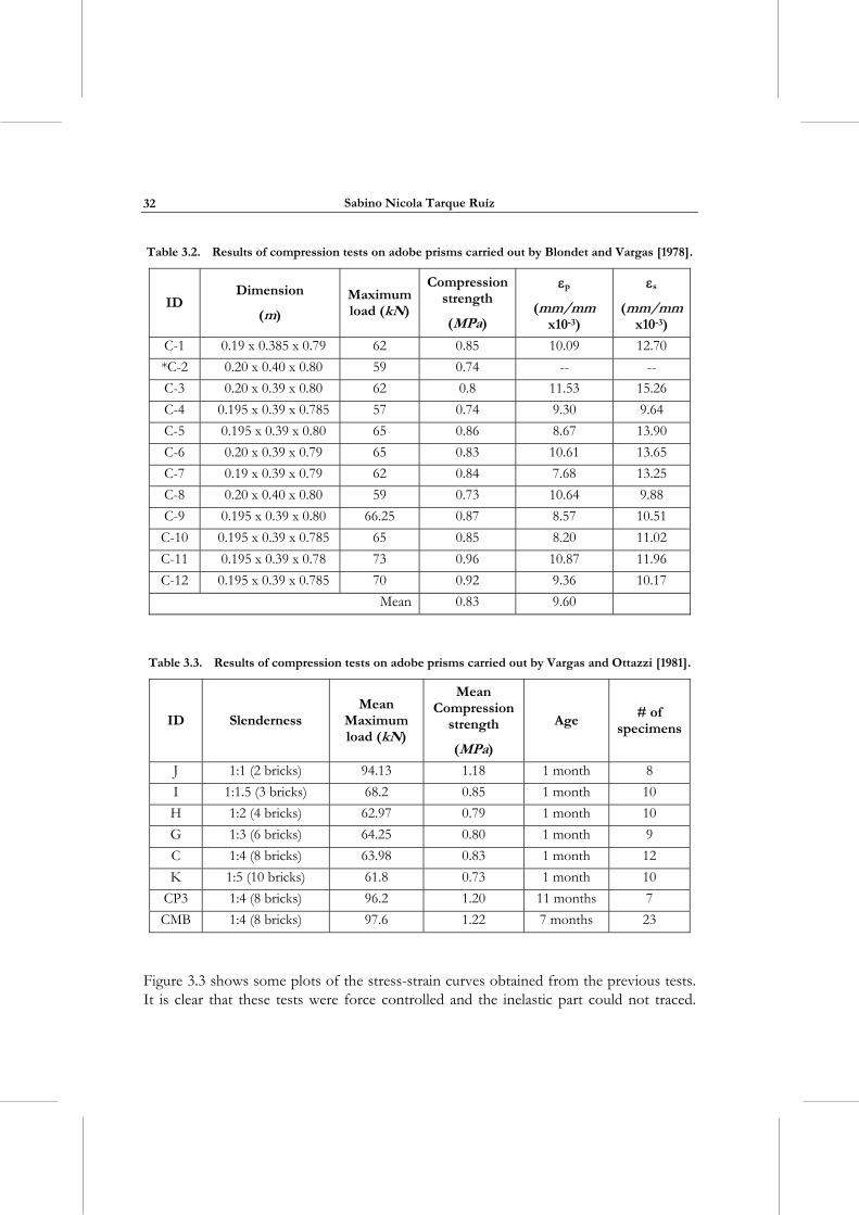
Sabino Nicola Tarque Ruíz
32
Table 3.2. Results of compression tests on adobe prisms carried out by Blondet and Vargas [1978].
ID Dimension
(m)
Maximum load (kN)
Compression strength
(MPa)
p
(mm/mm x10-3)
s
(mm/mm x10-3)
C-1 0.19 x 0.385 x 0.79 62 0.85 10.09 12.70
*C-2 0.20 x 0.40 x 0.80 59 0.74 -- --
C-3 0.20 x 0.39 x 0.80 62 0.8 11.53 15.26
C-4 0.195 x 0.39 x 0.785 57 0.74 9.30 9.64
C-5 0.195 x 0.39 x 0.80 65 0.86 8.67 13.90
C-6 0.20 x 0.39 x 0.79 65 0.83 10.61 13.65
C-7 0.19 x 0.39 x 0.79 62 0.84 7.68 13.25
C-8 0.20 x 0.40 x 0.80 59 0.73 10.64 9.88
C-9 0.195 x 0.39 x 0.80 66.25 0.87 8.57 10.51
C-10 0.195 x 0.39 x 0.785 65 0.85 8.20 11.02
C-11 0.195 x 0.39 x 0.78 73 0.96 10.87 11.96
C-12 0.195 x 0.39 x 0.785 70 0.92 9.36 10.17
Mean 0.83 9.60
Table 3.3. Results of compression tests on adobe prisms carried out by Vargas and Ottazzi [1981].
ID Slenderness Mean
Maximum load (kN)
Mean Compression
strength
(MPa)
Age # of
specimens
J 1:1 (2 bricks) 94.13 1.18 1 month 8
I 1:1.5 (3 bricks) 68.2 0.85 1 month 10
H 1:2 (4 bricks) 62.97 0.79 1 month 10
G 1:3 (6 bricks) 64.25 0.80 1 month 9
C 1:4 (8 bricks) 63.98 0.83 1 month 12
K 1:5 (10 bricks) 61.8 0.73 1 month 10
CP3 1:4 (8 bricks) 96.2 1.20 11 months 7
CMB 1:4 (8 bricks) 97.6 1.22 7 months 23
Figure 3.3 shows some plots of the stress-strain curves obtained from the previous tests. It is clear that these tests were force controlled and the inelastic part could not traced.
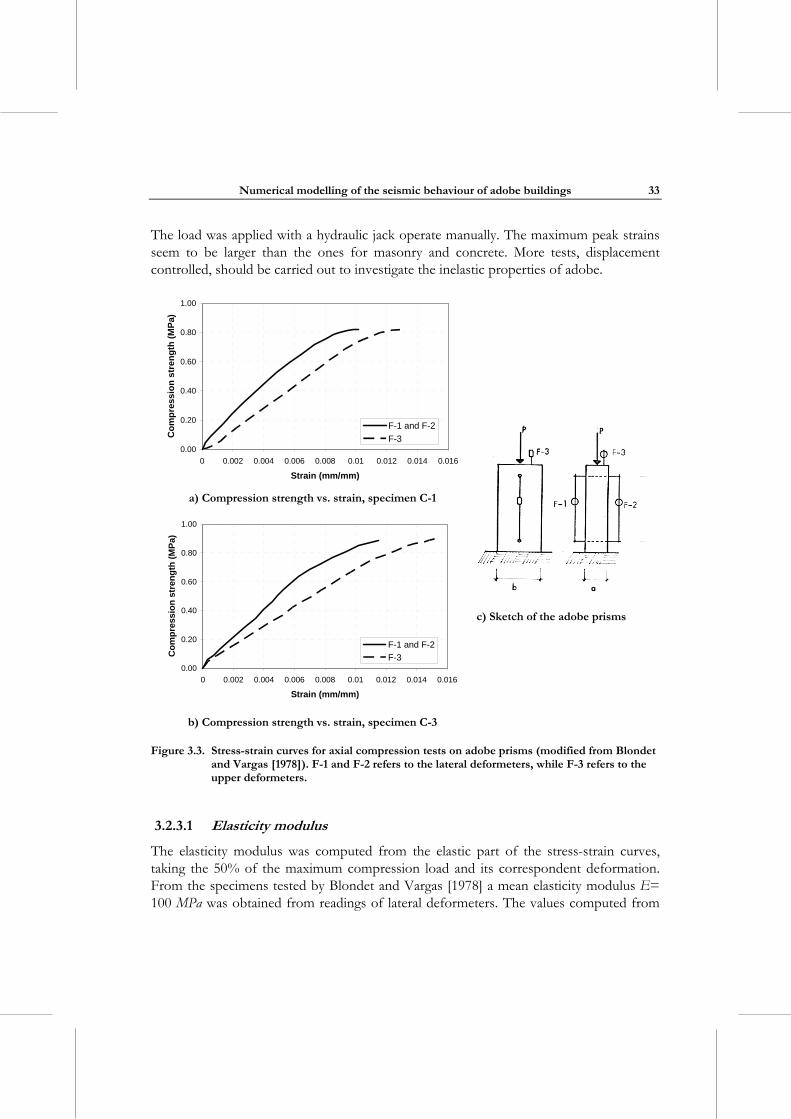
Numerical modelling of the seismic behaviour of adobe buildings
33
The load was applied with a hydraulic jack operate manually. The maximum peak strains seem to be larger than the ones for masonry and concrete. More tests, displacement controlled, should be carried out to investigate the inelastic properties of adobe.
0.00
0.20
0.40
0.60
0.80
1.00
0 0.002 0.004 0.006 0.008 0.01 0.012 0.014 0.016
Strain (mm/mm)
Co
mp
ress
ion
str
eng
th (
MP
a)
F-1 and F-2
F-3
a) Compression strength vs. strain, specimen C-1
0.00
0.20
0.40
0.60
0.80
1.00
0 0.002 0.004 0.006 0.008 0.01 0.012 0.014 0.016
Strain (mm/mm)
Co
mp
ress
ion
str
eng
th (
MP
a)
F-1 and F-2
F-3
c) Sketch of the adobe prisms
b) Compression strength vs. strain, specimen C-3
Figure 3.3. Stress-strain curves for axial compression tests on adobe prisms (modified from Blondet and Vargas [1978]). F-1 and F-2 refers to the lateral deformeters, while F-3 refers to the upper deformeters.
3.2.3.1 Elasticity modulus
The elasticity modulus was computed from the elastic part of the stress-strain curves, taking the 50% of the maximum compression load and its correspondent deformation. From the specimens tested by Blondet and Vargas [1978] a mean elasticity modulus E= 100 MPa was obtained from readings of lateral deformeters. The values computed from
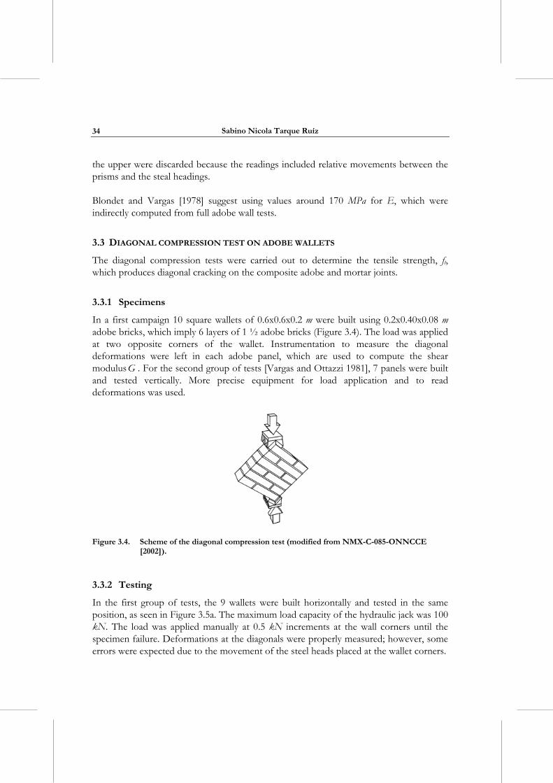
Sabino Nicola Tarque Ruíz
34
the upper were discarded because the readings included relative movements between the prisms and the steal headings.
Blondet and Vargas [1978] suggest using values around 170 MPa for E, which were indirectly computed from full adobe wall tests.
3.3 DIAGONAL COMPRESSION TEST ON ADOBE WALLETS
The diagonal compression tests were carried out to determine the tensile strength, ft, which produces diagonal cracking on the composite adobe and mortar joints.
3.3.1 Specimens
In a first campaign 10 square wallets of 0.6x0.6x0.2 m were built using 0.2x0.40x0.08 m adobe bricks, which imply 6 layers of 1 ½ adobe bricks (Figure 3.4). The load was applied at two opposite corners of the wallet. Instrumentation to measure the diagonal deformations were left in each adobe panel, which are used to compute the shear modulusG . For the second group of tests [Vargas and Ottazzi 1981], 7 panels were built and tested vertically. More precise equipment for load application and to read deformations was used.
Figure 3.4. Scheme of the diagonal compression test (modified from NMX-C-085-ONNCCE
[2002]).
3.3.2 Testing
In the first group of tests, the 9 wallets were built horizontally and tested in the same position, as seen in Figure 3.5a. The maximum load capacity of the hydraulic jack was 100 kN. The load was applied manually at 0.5 kN increments at the wall corners until the specimen failure. Deformations at the diagonals were properly measured; however, some errors were expected due to the movement of the steel heads placed at the wallet corners.
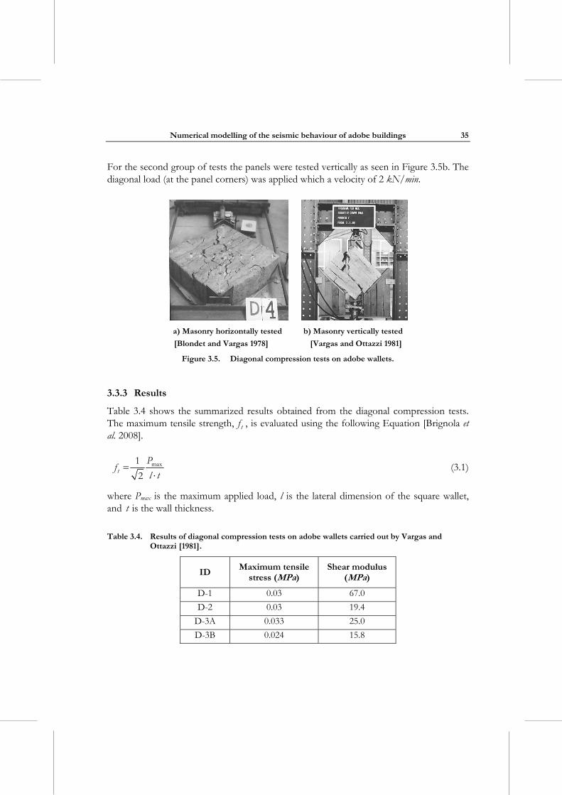
Numerical modelling of the seismic behaviour of adobe buildings
35
For the second group of tests the panels were tested vertically as seen in Figure 3.5b. The diagonal load (at the panel corners) was applied which a velocity of 2 kN/min.
a) Masonry horizontally tested b) Masonry vertically tested
[Blondet and Vargas 1978] [Vargas and Ottazzi 1981]
Figure 3.5. Diagonal compression tests on adobe wallets.
3.3.3 Results
Table 3.4 shows the summarized results obtained from the diagonal compression tests. The maximum tensile strength, tf , is evaluated using the following Equation [Brignola et al. 2008].
t
Pf
l tmax1
2
(3.1)
where Pmax is the maximum applied load, l is the lateral dimension of the square wallet, and t is the wall thickness.
Table 3.4. Results of diagonal compression tests on adobe wallets carried out by Vargas and Ottazzi [1981].
ID Maximum tensile
stress (MPa) Shear modulus
(MPa)
D-1 0.03 67.0
D-2 0.03 19.4
D-3A 0.033 25.0
D-3B 0.024 15.8
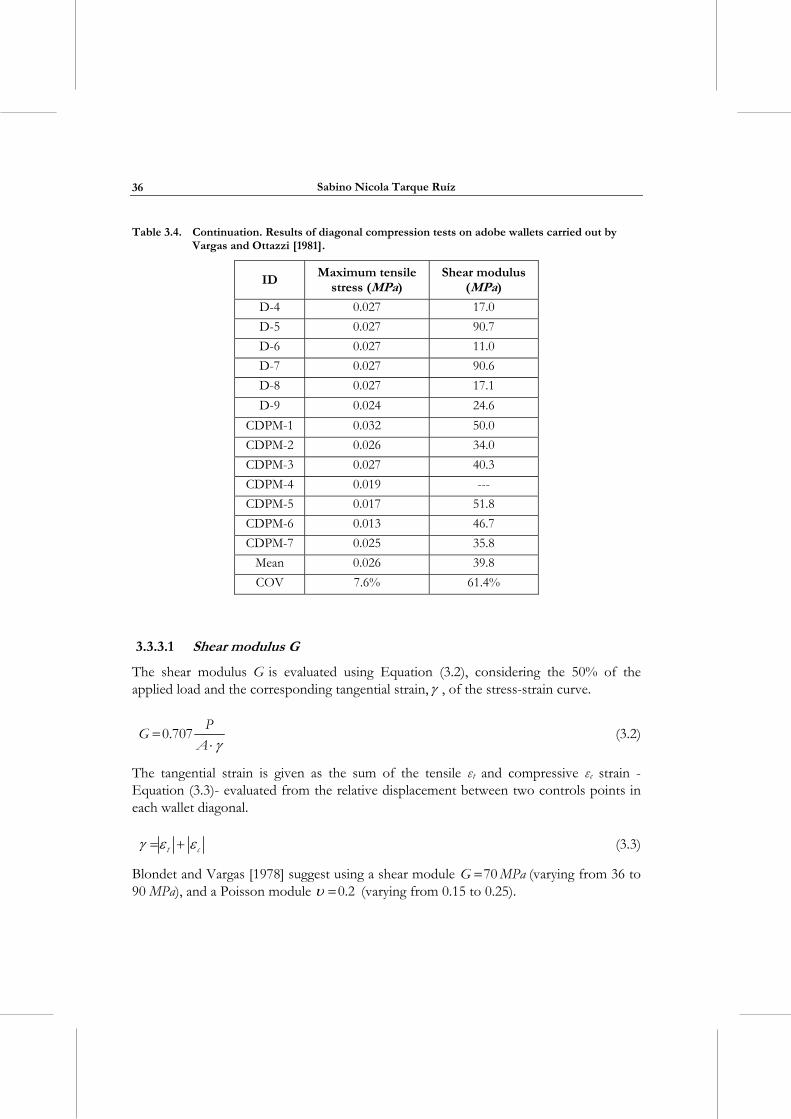
Sabino Nicola Tarque Ruíz
36
Table 3.4. Continuation. Results of diagonal compression tests on adobe wallets carried out by Vargas and Ottazzi [1981].
ID Maximum tensile
stress (MPa) Shear modulus
(MPa)
D-4 0.027 17.0
D-5 0.027 90.7
D-6 0.027 11.0
D-7 0.027 90.6
D-8 0.027 17.1
D-9 0.024 24.6
CDPM-1 0.032 50.0
CDPM-2 0.026 34.0
CDPM-3 0.027 40.3
CDPM-4 0.019 ---
CDPM-5 0.017 51.8
CDPM-6 0.013 46.7
CDPM-7 0.025 35.8
Mean 0.026 39.8
COV 7.6% 61.4%
3.3.3.1 Shear modulus G
The shear modulus G is evaluated using Equation (3.2), considering the 50% of the applied load and the corresponding tangential strain, , of the stress-strain curve.
PG
A0.707
(3.2)
The tangential strain is given as the sum of the tensile εt and compressive εc strain -Equation (3.3)- evaluated from the relative displacement between two controls points in each wallet diagonal.
t c (3.3)
Blondet and Vargas [1978] suggest using a shear module G MPa70 (varying from 36 to 90 MPa), and a Poisson module 0.2 (varying from 0.15 to 0.25).
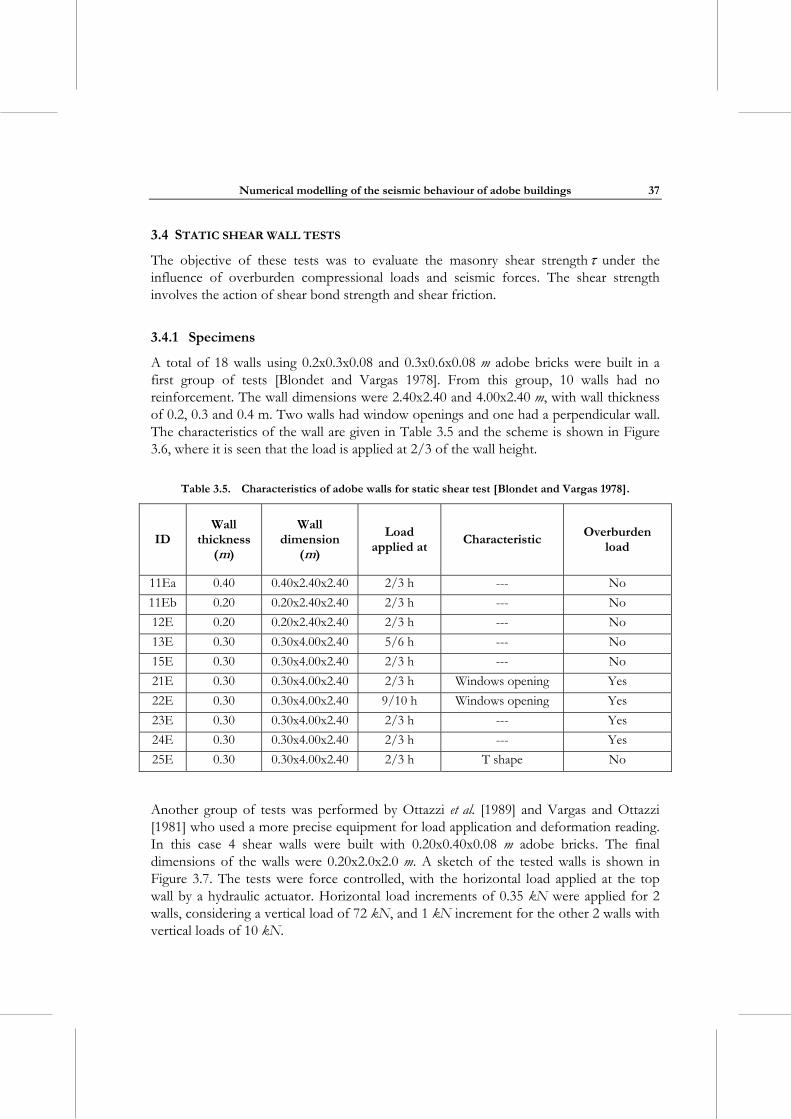
Numerical modelling of the seismic behaviour of adobe buildings
37
3.4 STATIC SHEAR WALL TESTS
The objective of these tests was to evaluate the masonry shear strength under the influence of overburden compressional loads and seismic forces. The shear strength involves the action of shear bond strength and shear friction.
3.4.1 Specimens
A total of 18 walls using 0.2x0.3x0.08 and 0.3x0.6x0.08 m adobe bricks were built in a first group of tests [Blondet and Vargas 1978]. From this group, 10 walls had no reinforcement. The wall dimensions were 2.40x2.40 and 4.00x2.40 m, with wall thickness of 0.2, 0.3 and 0.4 m. Two walls had window openings and one had a perpendicular wall. The characteristics of the wall are given in Table 3.5 and the scheme is shown in Figure 3.6, where it is seen that the load is applied at 2/3 of the wall height.
Table 3.5. Characteristics of adobe walls for static shear test [Blondet and Vargas 1978].
ID Wall
thickness (m)
Wall dimension
(m)
Load applied at
Characteristic Overburden
load
11Ea 0.40 0.40x2.40x2.40 2/3 h --- No
11Eb 0.20 0.20x2.40x2.40 2/3 h --- No
12E 0.20 0.20x2.40x2.40 2/3 h --- No
13E 0.30 0.30x4.00x2.40 5/6 h --- No
15E 0.30 0.30x4.00x2.40 2/3 h --- No
21E 0.30 0.30x4.00x2.40 2/3 h Windows opening Yes
22E 0.30 0.30x4.00x2.40 9/10 h Windows opening Yes
23E 0.30 0.30x4.00x2.40 2/3 h --- Yes
24E 0.30 0.30x4.00x2.40 2/3 h --- Yes
25E 0.30 0.30x4.00x2.40 2/3 h T shape No
Another group of tests was performed by Ottazzi et al. [1989] and Vargas and Ottazzi [1981] who used a more precise equipment for load application and deformation reading. In this case 4 shear walls were built with 0.20x0.40x0.08 m adobe bricks. The final dimensions of the walls were 0.20x2.0x2.0 m. A sketch of the tested walls is shown in Figure 3.7. The tests were force controlled, with the horizontal load applied at the top wall by a hydraulic actuator. Horizontal load increments of 0.35 kN were applied for 2 walls, considering a vertical load of 72 kN, and 1 kN increment for the other 2 walls with vertical loads of 10 kN.
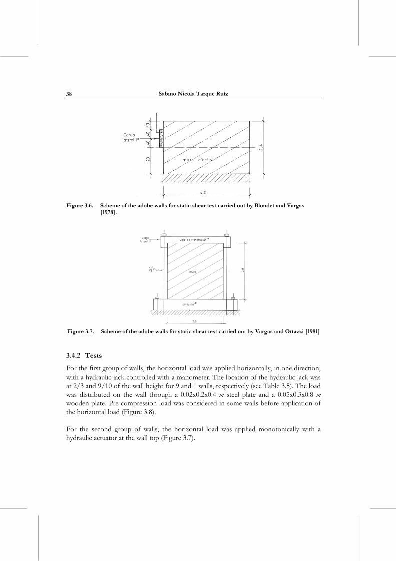
Sabino Nicola Tarque Ruíz
38
Figure 3.6. Scheme of the adobe walls for static shear test carried out by Blondet and Vargas
[1978].
Figure 3.7. Scheme of the adobe walls for static shear test carried out by Vargas and Ottazzi [1981]
3.4.2 Tests
For the first group of walls, the horizontal load was applied horizontally, in one direction, with a hydraulic jack controlled with a manometer. The location of the hydraulic jack was at 2/3 and 9/10 of the wall height for 9 and 1 walls, respectively (see Table 3.5). The load was distributed on the wall through a 0.02x0.2x0.4 m steel plate and a 0.05x0.3x0.8 m wooden plate. Pre compression load was considered in some walls before application of the horizontal load (Figure 3.8).
For the second group of walls, the horizontal load was applied monotonically with a hydraulic actuator at the wall top (Figure 3.7).
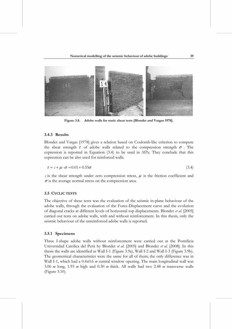
Numerical modelling of the seismic behaviour of adobe buildings
39
Figure 3.8. Adobe walls for static shear tests [Blondet and Vargas 1978].
3.4.3 Results
Blondet and Vargas [1978] gives a relation based on Coulomb-like criterion to compute the shear strength of adobe walls related to the compression strength . The expression is reported in Equation (3.4) to be used in MPa. They conclude that this expression can be also used for reinforced walls.
c 0.01 0.55 (3.4)
c is the shear strength under zero compression stress, is the friction coefficient and is the average normal stress on the compression area.
3.5 CYCLIC TESTS
The objective of these tests was the evaluation of the seismic in-plane behaviour of the adobe walls, through the evaluation of the Force-Displacement curve and the evolution of diagonal cracks at different levels of horizontal top displacements. Blondet et al. [2005] carried out tests on adobe walls, with and without reinforcement. In this thesis, only the seismic behaviour of the unreinforced adobe walls is reported.
3.5.1 Specimens
Three I-shape adobe walls without reinforcement were carried out at the Pontificia Universidad Católica del Perú by Blondet et al. [2005] and Blondet et al. [2008]. In this thesis the walls are identified as Wall I-1 (Figure 3.9a), Wall I-2 and Wall I-3 (Figure 3.9b). The geometrical characteristics were the same for all of them; the only difference was in Wall I-1, which had a 0.4x0.6 m central window opening. The main longitudinal wall was 3.06 m long, 1.93 m high and 0.30 m thick. All walls had two 2.48 m transverse walls (Figure 3.10).
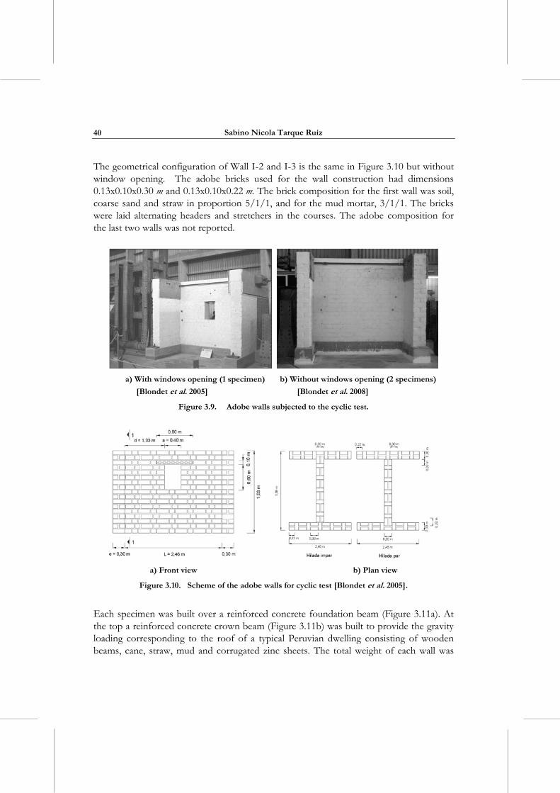
Sabino Nicola Tarque Ruíz
40
The geometrical configuration of Wall I-2 and I-3 is the same in Figure 3.10 but without window opening. The adobe bricks used for the wall construction had dimensions 0.13x0.10x0.30 m and 0.13x0.10x0.22 m. The brick composition for the first wall was soil, coarse sand and straw in proportion 5/1/1, and for the mud mortar, 3/1/1. The bricks were laid alternating headers and stretchers in the courses. The adobe composition for the last two walls was not reported.
a) With windows opening (1 specimen) b) Without windows opening (2 specimens)
[Blondet et al. 2005] [Blondet et al. 2008]
Figure 3.9. Adobe walls subjected to the cyclic test.
a) Front view b) Plan view
Figure 3.10. Scheme of the adobe walls for cyclic test [Blondet et al. 2005].
Each specimen was built over a reinforced concrete foundation beam (Figure 3.11a). At the top a reinforced concrete crown beam (Figure 3.11b) was built to provide the gravity loading corresponding to the roof of a typical Peruvian dwelling consisting of wooden beams, cane, straw, mud and corrugated zinc sheets. The total weight of each wall was
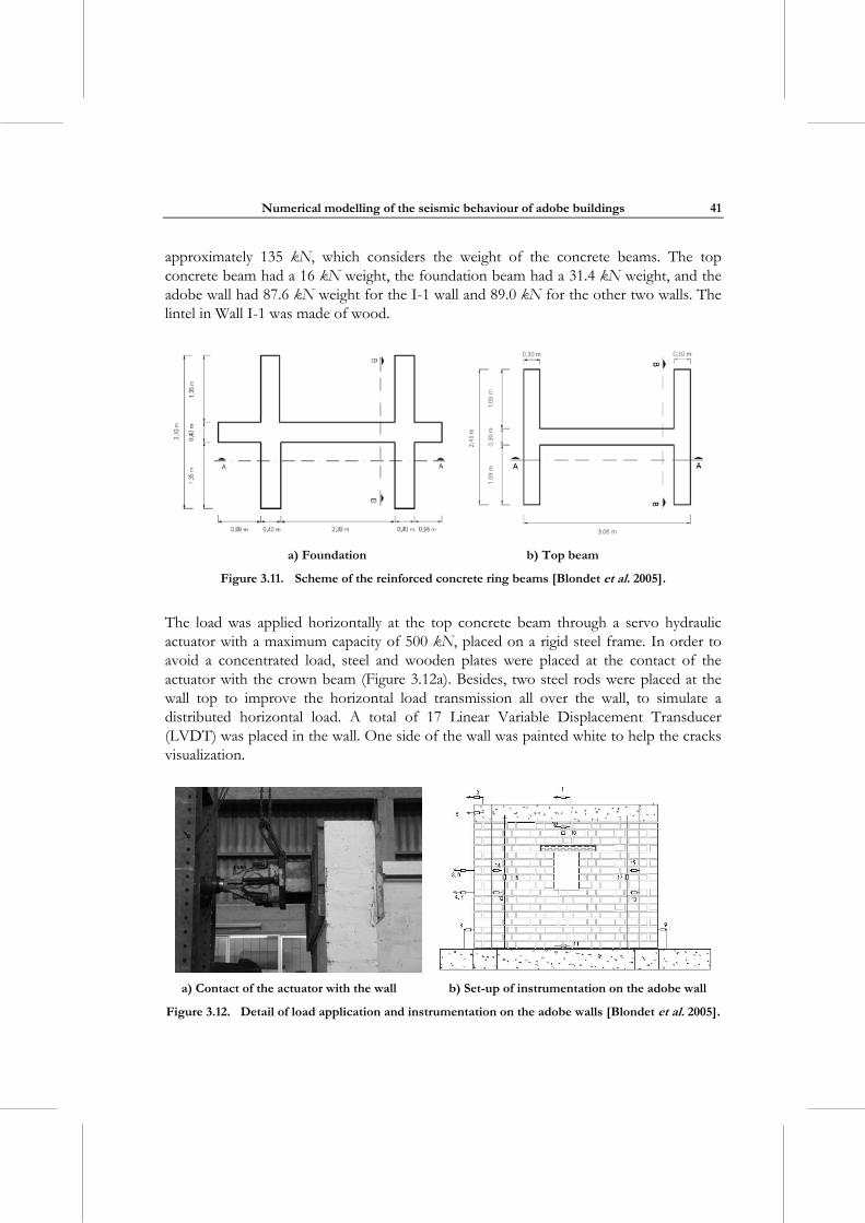
Numerical modelling of the seismic behaviour of adobe buildings
41
approximately 135 kN, which considers the weight of the concrete beams. The top concrete beam had a 16 kN weight, the foundation beam had a 31.4 kN weight, and the adobe wall had 87.6 kN weight for the I-1 wall and 89.0 kN for the other two walls. The lintel in Wall I-1 was made of wood.
a) Foundation b) Top beam
Figure 3.11. Scheme of the reinforced concrete ring beams [Blondet et al. 2005].
The load was applied horizontally at the top concrete beam through a servo hydraulic actuator with a maximum capacity of 500 kN, placed on a rigid steel frame. In order to avoid a concentrated load, steel and wooden plates were placed at the contact of the actuator with the crown beam (Figure 3.12a). Besides, two steel rods were placed at the wall top to improve the horizontal load transmission all over the wall, to simulate a distributed horizontal load. A total of 17 Linear Variable Displacement Transducer (LVDT) was placed in the wall. One side of the wall was painted white to help the cracks visualization.
a) Contact of the actuator with the wall b) Set-up of instrumentation on the adobe wall
Figure 3.12. Detail of load application and instrumentation on the adobe walls [Blondet et al. 2005].
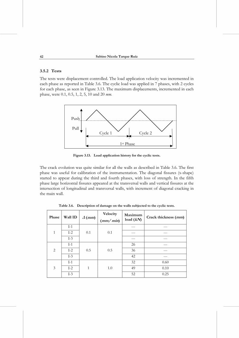
Sabino Nicola Tarque Ruíz
42
3.5.2 Tests
The tests were displacement controlled. The load application velocity was incremented in each phase as reported in Table 3.6. The cyclic load was applied in 7 phases, with 2 cycles for each phase, as seen in Figure 3.13. The maximum displacements, incremented in each phase, were 0.1, 0.5, 1, 2, 5, 10 and 20 mm.
Figure 3.13. Load application history for the cyclic tests.
The crack evolution was quite similar for all the walls as described in Table 3.6. The first phase was useful for calibration of the instrumentation. The diagonal fissures (x-shape) started to appear during the third and fourth phases, with loss of strength. In the fifth phase large horizontal fissures appeared at the transversal walls and vertical fissures at the intersection of longitudinal and transversal walls, with increment of diagonal cracking in the main wall.
Table 3.6. Description of damage on the walls subjected to the cyclic tests.
Phase Wall ID (mm) Velocity
(mm/ min)
Maximum load (kN)
Crack thickness (mm)
I-1 --- ---
I-2 --- --- 1
I-3
0.1 0.1
--- ---
I-1 26 ---
I-2 36 --- 2
I-3
0.5 0.5
42 ---
I-1 32 0.60
I-2 49 0.10 3
I-3
1 1.0
52 0.25
Cycle 1 Cycle 2
1st Phase
Push
Pull
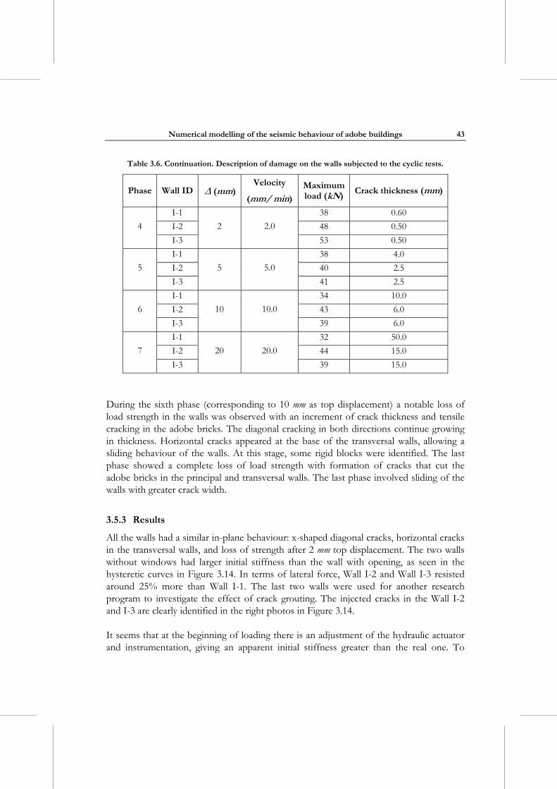
Numerical modelling of the seismic behaviour of adobe buildings
43
Table 3.6. Continuation. Description of damage on the walls subjected to the cyclic tests.
Phase Wall ID (mm)Velocity
(mm/ min)
Maximum load (kN)
Crack thickness (mm)
I-1 38 0.60
I-2 48 0.50 4
I-3
2 2.0
53 0.50
I-1 38 4.0
I-2 40 2.5 5
I-3
5 5.0
41 2.5
I-1 34 10.0
I-2 43 6.0 6
I-3
10 10.0
39 6.0
I-1 32 50.0
I-2 44 15.0 7
I-3
20 20.0
39 15.0
During the sixth phase (corresponding to 10 mm as top displacement) a notable loss of load strength in the walls was observed with an increment of crack thickness and tensile cracking in the adobe bricks. The diagonal cracking in both directions continue growing in thickness. Horizontal cracks appeared at the base of the transversal walls, allowing a sliding behaviour of the walls. At this stage, some rigid blocks were identified. The last phase showed a complete loss of load strength with formation of cracks that cut the adobe bricks in the principal and transversal walls. The last phase involved sliding of the walls with greater crack width.
3.5.3 Results
All the walls had a similar in-plane behaviour: x-shaped diagonal cracks, horizontal cracks in the transversal walls, and loss of strength after 2 mm top displacement. The two walls without windows had larger initial stiffness than the wall with opening, as seen in the hysteretic curves in Figure 3.14. In terms of lateral force, Wall I-2 and Wall I-3 resisted around 25% more than Wall I-1. The last two walls were used for another research program to investigate the effect of crack grouting. The injected cracks in the Wall I-2 and I-3 are clearly identified in the right photos in Figure 3.14.
It seems that at the beginning of loading there is an adjustment of the hydraulic actuator and instrumentation, giving an apparent initial stiffness greater than the real one. To
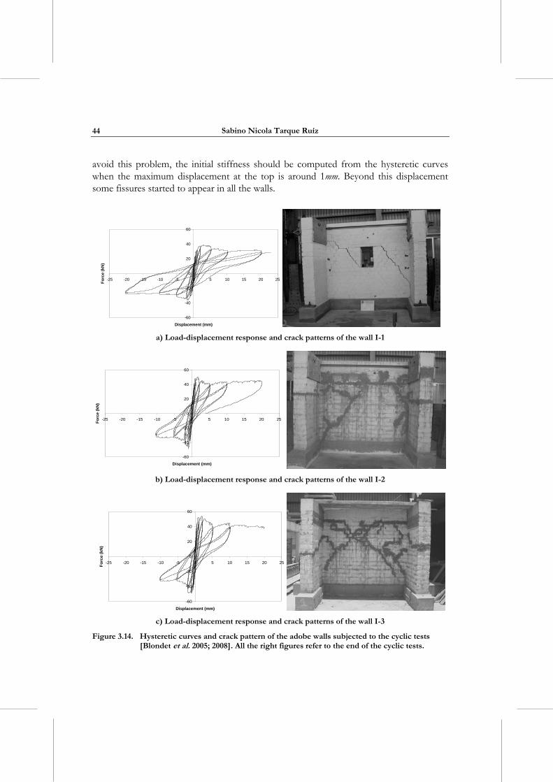
Sabino Nicola Tarque Ruíz
44
avoid this problem, the initial stiffness should be computed from the hysteretic curves when the maximum displacement at the top is around 1mm. Beyond this displacement some fissures started to appear in all the walls.
-60
-40
-20
0
20
40
60
-25 -20 -15 -10 -5 0 5 10 15 20 25
Displacement (mm)
Fo
rce
(kN
)
a) Load-displacement response and crack patterns of the wall I-1
-60
-40
-20
0
20
40
60
-25 -20 -15 -10 -5 0 5 10 15 20 25
Displacement (mm)
Fo
rce (
kN
)
b) Load-displacement response and crack patterns of the wall I-2
-60
-40
-20
0
20
40
60
-25 -20 -15 -10 -5 0 5 10 15 20 25
Displacement (mm)
Fo
rce
(kN
)
c) Load-displacement response and crack patterns of the wall I-3
Figure 3.14. Hysteretic curves and crack pattern of the adobe walls subjected to the cyclic tests [Blondet et al. 2005; 2008]. All the right figures refer to the end of the cyclic tests.
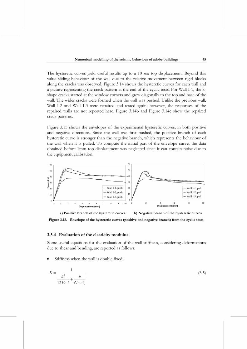
Numerical modelling of the seismic behaviour of adobe buildings
45
The hysteretic curves yield useful results up to a 10 mm top displacement. Beyond this value sliding behaviour of the wall due to the relative movement between rigid blocks along the cracks was observed. Figure 3.14 shows the hysteretic curves for each wall and a picture representing the crack pattern at the end of the cyclic tests. For Wall I-1, the x-shape cracks started at the window corners and grew diagonally to the top and base of the wall. The wider cracks were formed when the wall was pushed. Unlike the previous wall, Wall I-2 and Wall I-3 were repaired and tested again; however, the responses of the repaired walls are not reported here. Figure 3.14b and Figure 3.14c show the repaired crack patterns.
Figure 3.15 shows the envelopes of the experimental hysteretic curves, in both positive and negative directions. Since the wall was first pushed, the positive branch of each hysteretic curve is stronger than the negative branch, which represents the behaviour of the wall when it is pulled. To compute the initial part of the envelope curve, the data obtained before 1mm top displacement was neglected since it can contain noise due to the equipment calibration.
0
10
20
30
40
50
60
0 1 2 3 4 5 6 7 8 9 10
Displacement (mm)
Fo
rce
(kN
)
Wall I-1, push
Wall I-2, push
Wall I-3, push
0
10
20
30
40
50
60
0 2 4 6 8 10
Displacement (mm)
Wall I-1, pull
Wall I-2, pull
Wall I-3, pull
a) Positive branch of the hysteretic curves b) Negative branch of the hysteretic curves
Figure 3.15. Envelope of the hysteretic curves (positive and negative branch) from the cyclic tests.
3.5.4 Evaluation of the elasticity modulus
Some useful equations for the evaluation of the wall stiffness, considering deformations due to shear and bending, are reported as follows:
Stiffness when the wall is double fixed:
v
Kh hE I G A
3
1
12
(3.5)
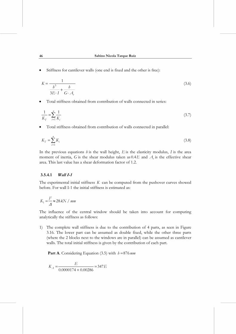
Sabino Nicola Tarque Ruíz
46
Stiffness for cantilever walls (one end is fixed and the other is free):
v
Kh hE I G A
3
1
3
(3.6)
Total stiffness obtained from contribution of walls connected in series:
n
iT iK K1
1 1
(3.7)
Total stiffness obtained from contribution of walls connected in parallel:
n
T ii
K K1
(3.8)
In the previous equations h is the wall height, E is the elasticity modulus, I is the area moment of inertia, G is the shear modulus taken as E0.4 and vA is the effective shear area. This last value has a shear deformation factor of 1.2.
3.5.4.1 Wall I-1
The experimental initial stiffness K can be computed from the pushover curves showed before. For wall I-1 the initial stiffness is estimated as:
FK kN mm1 28 /
The influence of the central window should be taken into account for computing analytically the stiffness as follows:
1) The complete wall stiffness is due to the contribution of 4 parts, as seen in Figure 3.16. The lower part can be assumed as double fixed, while the other three parts (where the 2 blocks next to the windows are in parallel) can be assumed as cantilever walls. The total initial stiffness is given by the contribution of each part.
Part A. Considering Equation (3.5) with h mm876
AE
K E3470.0000174 0.00286
Numerical modelling of the seismic behaviour of adobe buildings
47
It can be seen that the deformation due to bending is almost negligible. Therefore, considering a cantilever beam or a double fixed element will not influence the final evaluation of the initial stiffness. For Part A, considered as a cantilever beam, AK is 341E.
Figure 3.16. Scheme for evaluating the lateral stiffness of the adobe wall I-1.
Part B and Part C. Considering Equation (3.6) with h mm600
B CE
K K E219.10.00005564 0.004511
Again, it is seen that the influence of the bending deformation is small comparing it with the shear deformation. For Part B and C, considered as a double fixed beam,
BK is 221E.
Part D. Considering Equation (3.6) with h mm454
DE
K E6 669.79.87 10 0.00148
The total initial stiffness is computed combining Equations (3.7) and (3.8) as follows:
T A B C DK K K K K
1 1 1 1
Evaluating the previous equation, the total stiffness is TK E150 . So E MPa187
Sabino Nicola Tarque Ruíz
48
3.5.4.2 Wall I-2 and I-3
1) In this case there is not a window opening. The wall can be assumed as fixed at both ends with a distributed horizontal load at the top. The experimental initial stiffness computed from the pushover curves is around TK kN mm34 /
The area moment of inertia is:
I mm3 3
12 42480 3060 1090 24602 3.217 10
12 12
The effective shear area is given by the wall web:
v wA A mm25 52460 600 300 765000
6 6
Solving for Equation (3.5):
K E E/ 0.0001862 0.0063 154 . So, E MPa220 .
2) Rotation at the top part of the wall is accepted (cantilever beam); so, the initial stiffness is evaluating with Equation (3.6), resulting in E MPa240 .
3) Paulay and Priestley [1992] suggest to compute an effective width on wide-flanged walls to evaluate the seismic capacity of wall subjected to shear forces, as seen in Figure 3.17, this is based on the assumption that vertical forces due to shear stresses introduced by the web of the wall into the tension flange spread out at a slope of 1:2.
According to Figure 3.17, the effective width of the tension flange is expressed as:
eff w wb h b b (3.9)
where wh is the height wall, wb is the in-plane wall width and b is the length of the flange wall.
The effective width in compression is given by:
eff w wb h b b0.3 (3.10)
With the two expressions written above, the effective widths for the flanges are 2230 mm and 879 mm for the tension and compression zone, respectively.
The coordinates of the gravity centre along the application of the force is:
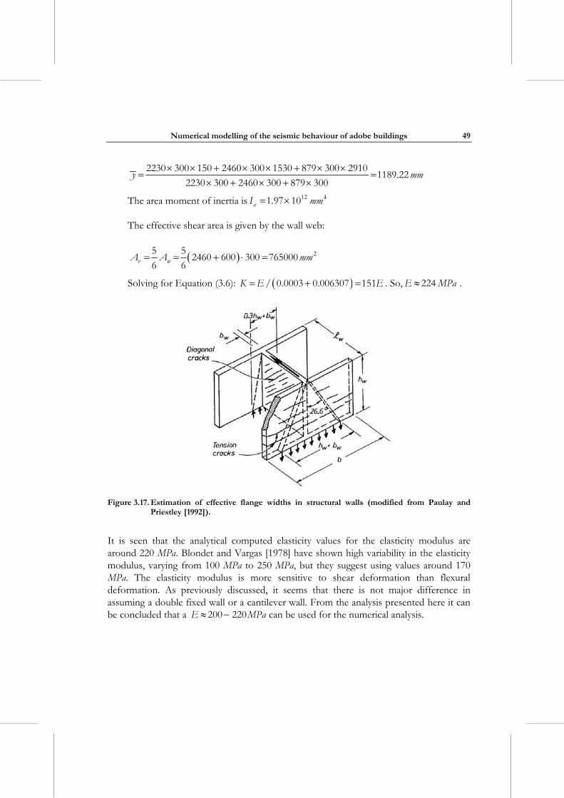
Numerical modelling of the seismic behaviour of adobe buildings
49
y mm2230 300 150 2460 300 1530 879 300 2910
1189.222230 300 2460 300 879 300
The area moment of inertia is aI mm12 41.97 10
The effective shear area is given by the wall web:
v wA A mm25 52460 600 300 765000
6 6
Solving for Equation (3.6): K E E/ 0.0003 0.006307 151 . So, E MPa224 .
Figure 3.17. Estimation of effective flange widths in structural walls (modified from Paulay and
Priestley [1992]).
It is seen that the analytical computed elasticity values for the elasticity modulus are around 220 MPa. Blondet and Vargas [1978] have shown high variability in the elasticity modulus, varying from 100 MPa to 250 MPa, but they suggest using values around 170 MPa. The elasticity modulus is more sensitive to shear deformation than flexural deformation. As previously discussed, it seems that there is not major difference in assuming a double fixed wall or a cantilever wall. From the analysis presented here it can be concluded that a E MPa200 220 can be used for the numerical analysis.
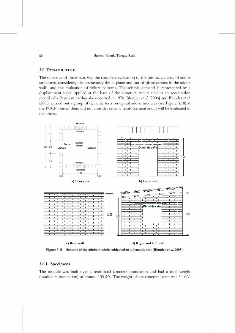
Sabino Nicola Tarque Ruíz
50
3.6 DYNAMIC TESTS
The objective of these tests was the complete evaluation of the seismic capacity of adobe structures, considering simultaneously the in-plane and out-of-plane actions in the adobe walls, and the evaluation of failure patterns. The seismic demand is represented by a displacement signal applied at the base of the structure and related to an acceleration record of a Peruvian earthquake occurred in 1970. Blondet et al. [2006] and Blondet et al. [2005] carried out a group of dynamic tests on typical adobe modules (see Figure 3.18) at the PUCP; one of them did not consider seismic reinforcement and it will be evaluated in this thesis.
MURO WMURO E
MURO N
MURO S
3.20
2.710.250.25
Ventana
Ventana
1.12
0.96
1.12
Puerta HILADAIMPAR
a) Plan view b) Front wall
c) Rear wall d) Right and left wall
Figure 3.18. Scheme of the adobe module subjected to a dynamic test [Blondet et al. 2005].
3.6.1 Specimens
The module was built over a reinforced concrete foundation and had a total weight (module + foundation) of around 135 kN. The weight of the concrete beam was 30 kN.
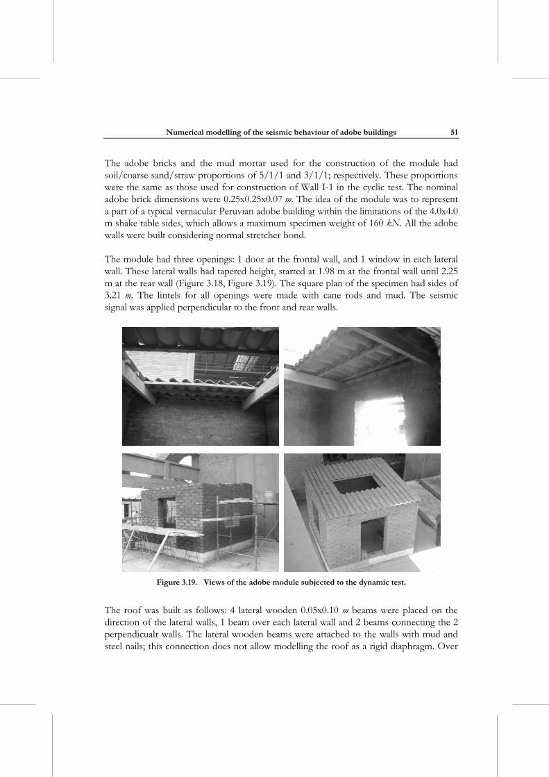
Numerical modelling of the seismic behaviour of adobe buildings
51
The adobe bricks and the mud mortar used for the construction of the module had soil/coarse sand/straw proportions of 5/1/1 and 3/1/1; respectively. These proportions were the same as those used for construction of Wall I-1 in the cyclic test. The nominal adobe brick dimensions were 0.25x0.25x0.07 m. The idea of the module was to represent a part of a typical vernacular Peruvian adobe building within the limitations of the 4.0x4.0 m shake table sides, which allows a maximum specimen weight of 160 kN. All the adobe walls were built considering normal stretcher bond.
The module had three openings: 1 door at the frontal wall, and 1 window in each lateral wall. These lateral walls had tapered height, started at 1.98 m at the frontal wall until 2.25 m at the rear wall (Figure 3.18, Figure 3.19). The square plan of the specimen had sides of 3.21 m. The lintels for all openings were made with cane rods and mud. The seismic signal was applied perpendicular to the front and rear walls.
Figure 3.19. Views of the adobe module subjected to the dynamic test.
The roof was built as follows: 4 lateral wooden 0.05x0.10 m beams were placed on the direction of the lateral walls, 1 beam over each lateral wall and 2 beams connecting the 2 perpendicualr walls. The lateral wooden beams were attached to the walls with mud and steel nails; this connection does not allow modelling the roof as a rigid diaphragm. Over
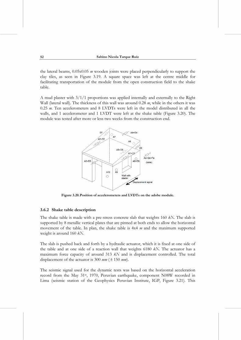
Sabino Nicola Tarque Ruíz
52
the lateral beams, 0.05x0.05 m wooden joints were placed perpendicularly to support the clay tiles, as seen in Figure 3.19. A square space was left at the centre middle for facilitating transportation of the module from the open construction field to the shake table.
A mud plaster with 3/1/1 proportions was applied internally and externally to the Right Wall (lateral wall). The thickness of this wall was around 0.28 m, while in the others it was 0.25 m. Ten accelerometers and 8 LVDTs were left in the model distributed in all the walls, and 1 accelerometer and 1 LVDT were left at the shake table (Figure 3.20). The module was tested after more or less two weeks from the construction end.
Figure 3.20. Position of accelerometers and LVDTs on the adobe module.
3.6.2 Shake table description
The shake table is made with a pre-stress concrete slab that weights 160 kN. The slab is supported by 8 metallic vertical plates that are pinned at both ends to allow the horizontal movement of the table. In plan, the shake table is 4x4 m and the maximum supported weight is around 160 kN.
The slab is pushed back and forth by a hydraulic actuator, which it is fixed at one side of the table and at one side of a reaction wall that weights 6180 kN. The actuator has a maximum force capacity of around 313 kN and is displacement controlled. The total displacement of the actuator is 300 mm ( 150 mm).
The seismic signal used for the dynamic tests was based on the horizontal acceleration record from the May 31st, 1970, Peruvian earthquake, component N08W recorded in Lima (seismic station of the Geophysics Peruvian Institute, IGP, Figure 3.21). This
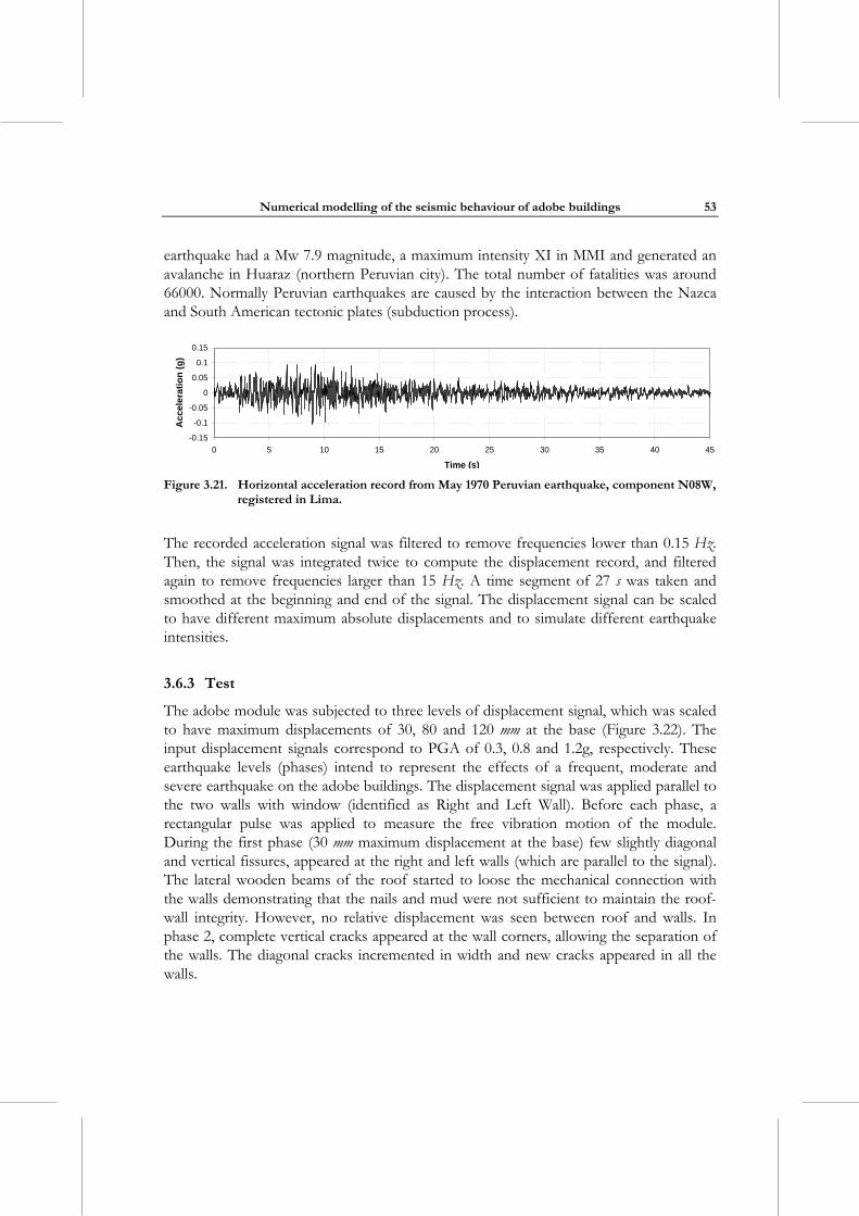
Numerical modelling of the seismic behaviour of adobe buildings
53
earthquake had a Mw 7.9 magnitude, a maximum intensity XI in MMI and generated an avalanche in Huaraz (northern Peruvian city). The total number of fatalities was around 66000. Normally Peruvian earthquakes are caused by the interaction between the Nazca and South American tectonic plates (subduction process).
-0.15
-0.1
-0.05
0
0.05
0.1
0.15
0 5 10 15 20 25 30 35 40 45
Time (s)
Acc
ele
rati
on
(g
)
Figure 3.21. Horizontal acceleration record from May 1970 Peruvian earthquake, component N08W,
registered in Lima.
The recorded acceleration signal was filtered to remove frequencies lower than 0.15 Hz. Then, the signal was integrated twice to compute the displacement record, and filtered again to remove frequencies larger than 15 Hz. A time segment of 27 s was taken and smoothed at the beginning and end of the signal. The displacement signal can be scaled to have different maximum absolute displacements and to simulate different earthquake intensities.
3.6.3 Test
The adobe module was subjected to three levels of displacement signal, which was scaled to have maximum displacements of 30, 80 and 120 mm at the base (Figure 3.22). The input displacement signals correspond to PGA of 0.3, 0.8 and 1.2g, respectively. These earthquake levels (phases) intend to represent the effects of a frequent, moderate and severe earthquake on the adobe buildings. The displacement signal was applied parallel to the two walls with window (identified as Right and Left Wall). Before each phase, a rectangular pulse was applied to measure the free vibration motion of the module. During the first phase (30 mm maximum displacement at the base) few slightly diagonal and vertical fissures, appeared at the right and left walls (which are parallel to the signal). The lateral wooden beams of the roof started to loose the mechanical connection with the walls demonstrating that the nails and mud were not sufficient to maintain the roof-wall integrity. However, no relative displacement was seen between roof and walls. In phase 2, complete vertical cracks appeared at the wall corners, allowing the separation of the walls. The diagonal cracks incremented in width and new cracks appeared in all the walls.
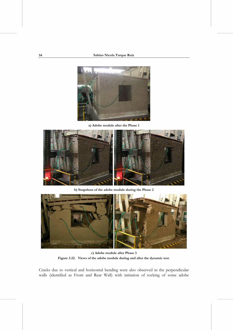
Sabino Nicola Tarque Ruíz
54
a) Adobe module after the Phase 1
b) Snapshots of the adobe module during the Phase 2
c) Adobe module after Phase 3
Figure 3.22. Views of the adobe module during and after the dynamic test.
Cracks due to vertical and horizontal bending were also observed in the perpendicular walls (identified as Front and Rear Wall) with initiation of rocking of some adobe
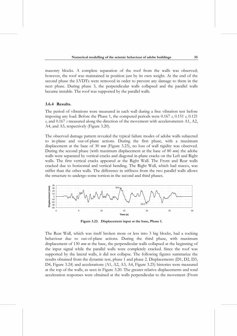
Numerical modelling of the seismic behaviour of adobe buildings
55
masonry blocks. A complete separation of the roof from the walls was observed; however, the roof was maintained in position just by its own weight. At the end of the second phase the LVDTs were removed in order to prevent any damage to them in the next phase. During phase 3, the perpendicular walls collapsed and the parallel walls became instable. The roof was supported by the parallel walls.
3.6.4 Results.
The period of vibrations were measured in each wall during a free vibration test before imposing any load. Before the Phase 1, the computed periods were 0.167 s, 0.151 s, 0.121 s, and 0.167 s measured along the direction of the movement with accelerometers A1, A2, A4, and A5, respectively (Figure 3.20). The observed damage pattern revealed the typical failure modes of adobe walls subjected to in-plane and out-of-plane actions. During the first phase, with a maximum displacement at the base of 30 mm (Figure 3.23), no loss of wall rigidity was observed. During the second phase (with maximum displacement at the base of 80 mm) the adobe walls were separated by vertical cracks and diagonal in-plane cracks on the Left and Right walls. The first vertical cracks appeared at the Right Wall. The Front and Rear walls cracked due to horizontal and vertical bending. The Right Wall, which had stucco, was stiffer than the other walls. The difference in stiffness from the two parallel walls allows the structure to undergo some torsion in the second and third phases.
-40-30-20-10
010203040
0 5 10 15 20 25 30
Time (s)
Dis
pla
cem
ent
(mm
)
-23.0
30.6
Figure 3.23. Displacement input at the base, Phase 1.
The Rear Wall, which was itself broken more or less into 3 big blocks, had a rocking behaviour due to out-of-plane actions. During the third phase, with maximum displacement of 130 mm at the base, the perpendicular walls collapsed at the beginning of the input signal while the parallel walls were completely cracked. Since the roof was supported by the lateral walls, it did not collapse. The following figures summarize the results obtained from the dynamic test, phase 1 and phase 2. Displacements (D1, D2, D3, D4, Figure 3.24) and accelerations (A1, A2, A3, A4, Figure 3.25) histories were measured at the top of the walls, as seen in Figure 3.20. The greater relative displacements and total acceleration responses were obtained at the walls perpendicular to the movement (Front
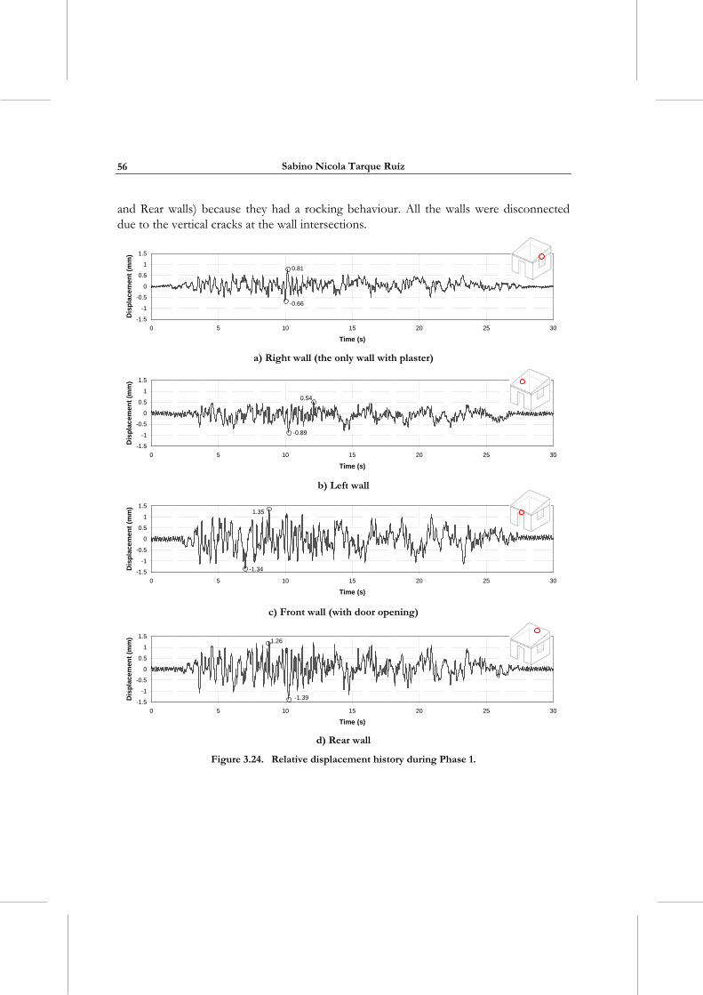
Sabino Nicola Tarque Ruíz
56
and Rear walls) because they had a rocking behaviour. All the walls were disconnected due to the vertical cracks at the wall intersections.
-1.5
-1
-0.5
0
0.5
1
1.5
0 5 10 15 20 25 30
Time (s)
Dis
pla
cem
ent
(mm
)
-0.66
0.81
a) Right wall (the only wall with plaster)
-1.5
-1
-0.5
0
0.5
1
1.5
0 5 10 15 20 25 30
Time (s)
Dis
pla
cem
ent
(mm
)
-0.89
0.54
b) Left wall
-1.5
-1
-0.5
0
0.5
1
1.5
0 5 10 15 20 25 30
Time (s)
Dis
pla
cem
ent
(mm
)
-1.34
1.35
c) Front wall (with door opening)
-1.5
-1
-0.5
0
0.5
1
1.5
0 5 10 15 20 25 30
Time (s)
Dis
pla
cem
ent
(mm
)
-1.39
1.26
d) Rear wall
Figure 3.24. Relative displacement history during Phase 1.
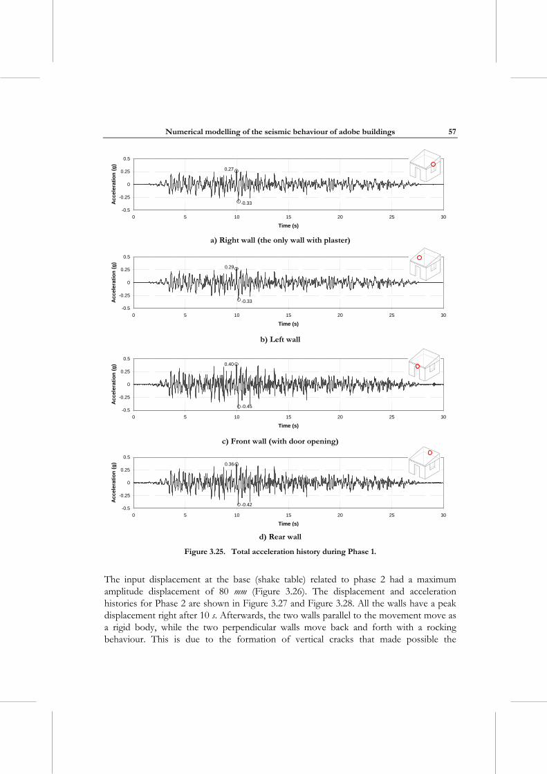
Numerical modelling of the seismic behaviour of adobe buildings
57
-0.5
-0.25
0
0.25
0.5
0 5 10 15 20 25 30
Time (s)
Acc
eler
atio
n (
g)
-0.33
0.27
a) Right wall (the only wall with plaster)
-0.5
-0.25
0
0.25
0.5
0 5 10 15 20 25 30
Time (s)
Acc
eler
atio
n (
g)
-0.33
0.29
b) Left wall
-0.5
-0.25
0
0.25
0.5
0 5 10 15 20 25 30
Time (s)
Acc
eler
ati
on
(g
)
-0.45
0.40
c) Front wall (with door opening)
-0.5
-0.25
0
0.25
0.5
0 5 10 15 20 25 30
Time (s)
Acc
eler
atio
n (
g)
-0.42
0.36
d) Rear wall
Figure 3.25. Total acceleration history during Phase 1.
The input displacement at the base (shake table) related to phase 2 had a maximum amplitude displacement of 80 mm (Figure 3.26). The displacement and acceleration histories for Phase 2 are shown in Figure 3.27 and Figure 3.28. All the walls have a peak displacement right after 10 s. Afterwards, the two walls parallel to the movement move as a rigid body, while the two perpendicular walls move back and forth with a rocking behaviour. This is due to the formation of vertical cracks that made possible the
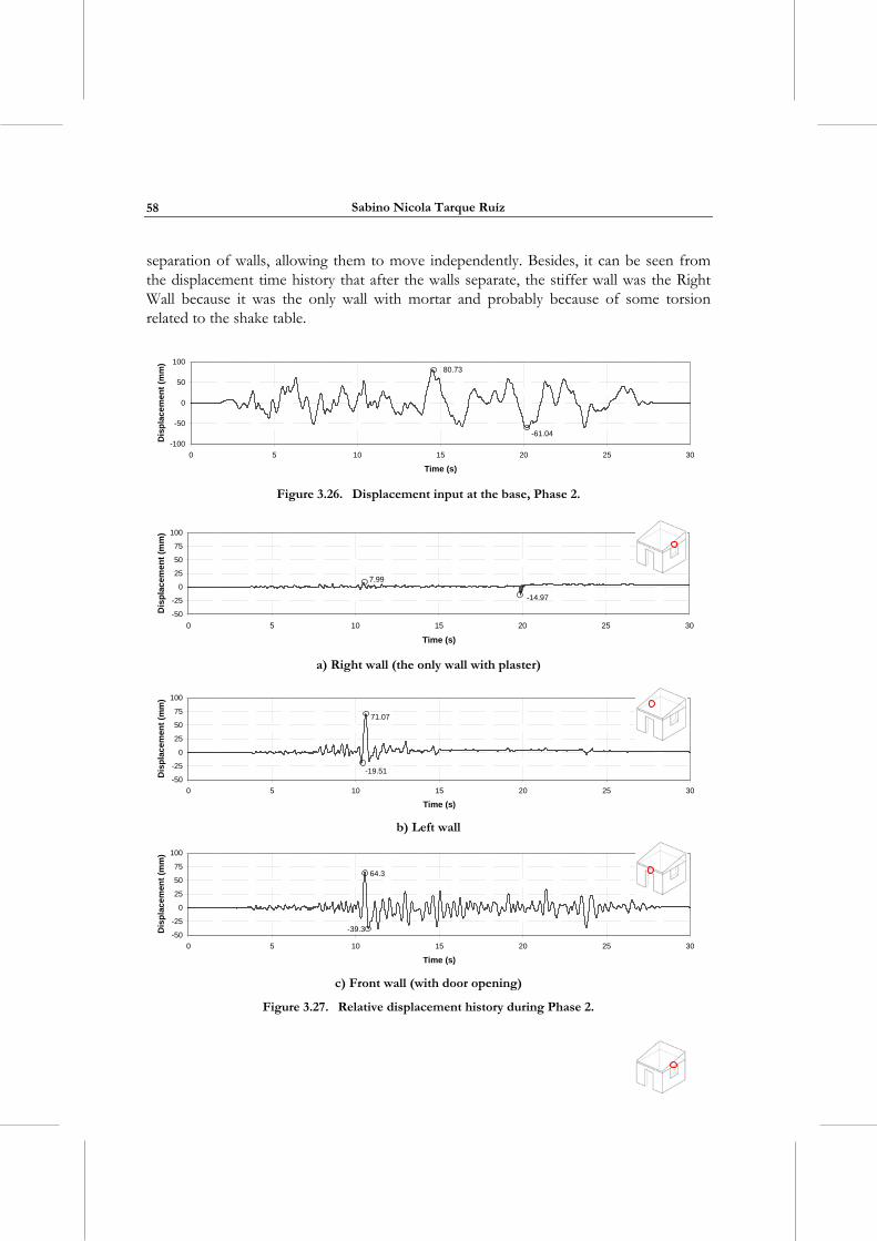
Sabino Nicola Tarque Ruíz
58
separation of walls, allowing them to move independently. Besides, it can be seen from the displacement time history that after the walls separate, the stiffer wall was the Right Wall because it was the only wall with mortar and probably because of some torsion related to the shake table.
-100
-50
0
50
100
0 5 10 15 20 25 30
Time (s)
Dis
pla
cem
ent
(mm
)
80.73
-61.04
Figure 3.26. Displacement input at the base, Phase 2.
-50
-25
0
25
50
75
100
0 5 10 15 20 25 30
Time (s)
Dis
pla
cem
ent
(mm
)
-14.97
7.99
a) Right wall (the only wall with plaster)
-50
-25
0
25
50
75
100
0 5 10 15 20 25 30
Time (s)
Dis
pla
cem
ent
(mm
)
-19.51
71.07
b) Left wall
-50
-25
0
25
50
75
100
0 5 10 15 20 25 30
Time (s)
Dis
pla
cem
ent
(mm
)
-39.3
64.3
c) Front wall (with door opening)
Figure 3.27. Relative displacement history during Phase 2.
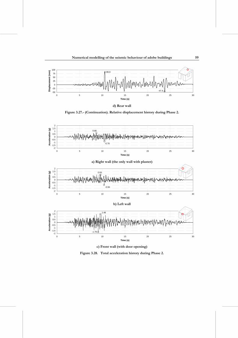
Numerical modelling of the seismic behaviour of adobe buildings
59
-50
-25
0
25
50
75
100
0 5 10 15 20 25 30
Time (s)
Dis
pla
cem
en
t (m
m)
-47.4
86.8
d) Rear wall
Figure 3.27.- (Continuation). Relative displacement history during Phase 2.
-2-1.5
-1-0.5
00.5
11.5
2
0 5 10 15 20 25 30
Time (s)
Acc
eler
atio
n (
g)
-0.76
0.68
a) Right wall (the only wall with plaster)
-2-1.5
-1-0.5
00.5
11.5
2
0 5 10 15 20 25 30
Time (s)
Acc
eler
atio
n (
g)
-0.94
0.93
b) Left wall
-2-1.5
-1-0.5
00.5
11.5
2
0 5 10 15 20 25 30
Time (s)
Ac
cele
rati
on
(g
)
-1.79
1.48
c) Front wall (with door opening)
Figure 3.28. Total acceleration history during Phase 2.
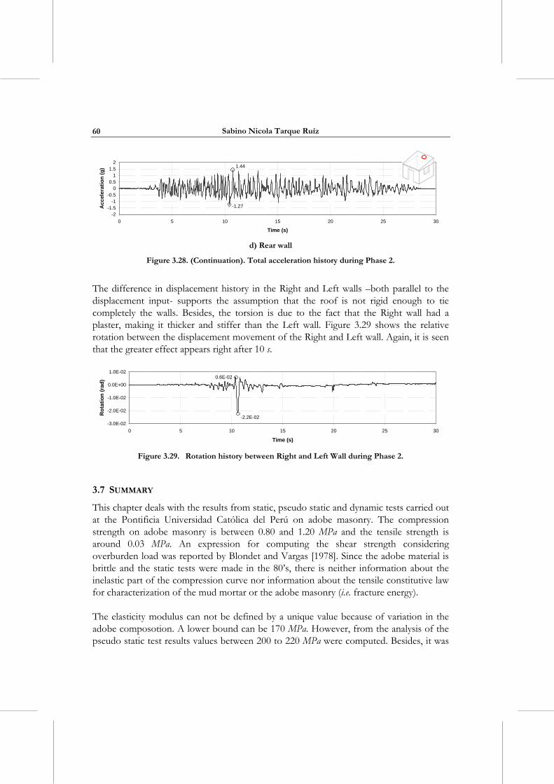
Sabino Nicola Tarque Ruíz
60
-2-1.5
-1-0.5
00.5
11.5
2
0 5 10 15 20 25 30
Time (s)
Acc
eler
atio
n (
g)
-1.27
1.44
d) Rear wall
Figure 3.28. (Continuation). Total acceleration history during Phase 2.
The difference in displacement history in the Right and Left walls –both parallel to the displacement input- supports the assumption that the roof is not rigid enough to tie completely the walls. Besides, the torsion is due to the fact that the Right wall had a plaster, making it thicker and stiffer than the Left wall. Figure 3.29 shows the relative rotation between the displacement movement of the Right and Left wall. Again, it is seen that the greater effect appears right after 10 s.
-3.0E-02
-2.0E-02
-1.0E-02
0.0E+00
1.0E-02
0 5 10 15 20 25 30
Time (s)
Ro
tati
on
(ra
d)
-2.2E-02
0.6E-02
Figure 3.29. Rotation history between Right and Left Wall during Phase 2.
3.7 SUMMARY
This chapter deals with the results from static, pseudo static and dynamic tests carried out at the Pontificia Universidad Católica del Perú on adobe masonry. The compression strength on adobe masonry is between 0.80 and 1.20 MPa and the tensile strength is around 0.03 MPa. An expression for computing the shear strength considering overburden load was reported by Blondet and Vargas [1978]. Since the adobe material is brittle and the static tests were made in the 80’s, there is neither information about the inelastic part of the compression curve nor information about the tensile constitutive law for characterization of the mud mortar or the adobe masonry (i.e. fracture energy).
The elasticity modulus can not be defined by a unique value because of variation in the adobe composotion. A lower bound can be 170 MPa. However, from the analysis of the pseudo static test results values between 200 to 220 MPa were computed. Besides, it was
Numerical modelling of the seismic behaviour of adobe buildings
61
observed that the soil characteristics have a great influence on the strength of the adobe masonry.
From the dynamic tests it was observed that in a building the adobe walls behave quasi independently during earthquakes because of the lack of diaphragm effect. Vertical cracks allowed the loss of connection between perpendicular walls. Taking advantage of the results from the pseudo static and the dynamic test, numerical models of the adobe wall and adobe module are developed in the next chapters to calibrate the adobe material parameters, particularly at the inelastic range (e.g. fracture energy in tension and compression).

4. REVIEW OF NUMERICAL MODELS APPLIED TO MASONRY STRUCTURES
The numerical analysis of unreinforced masonry structures (URM) can be carried out using different methods such as limit analysis, finite element method and the discrete element method [e.g. Kappos et al. 2002; Lourenço 1996; Page 1978; Pelà 2008; Roca et al. 2010]. Another approach consists in idealizing the structure through an equivalent frame where each wall is discretized by a set of masonry panels (piers and spandrels) in which the non-linear response is concentrated [e.g. Calderini et al. 2009; Galasco et al. 2004; Gambarotta and Lagomarsino 1997a; b; Lagomarsino et al. 2007; Magenes and Della Fontana 1998]. Masonry is a composite material formed by bricks and mortar joints, which each of them having its own material properties. The mortar is normally weaker and softer than the bricks. However, failure of masonry may involve the crushing and tensile fracturing of masonry units in addition to the fracturing of mortar joints [Stavridis and Shing 2010]. Masonry usually refers to fired brick masonry, while adobe masonry refers to adobe bricks (raw earth).
In comparison to masonry (fired bricks) and reinforced concrete structures, few work have been carried out regarding the numerical modelling of adobe constructions. One of the reasons for the little work is the lack of reliable material properties for representing the adobe material in the inelastic range. [Furukawa and Ohta 2009] and [Cao and Watanabe 2004], for example, modelled adobe modules following a finite element approach (FEM) and a discrete element approach (DEM), respectively.
In this work, a finite element approach is followed for modelling adobe masonry following a micro and macro-modelling technique. Besides, the most relevant masonry modelling works are discussed.
4.1 FROM MICRO-MODELLING TO MACRO-MODELLING
In general, the analysis of masonry structures can be classified according to the order of accuracy [Lourenço 1996], Figure 4.1:
detailed-micro modelling. Bricks and mortar joints are represented by continuum elements, where the unit-mortar interface is represented by discontinuous elements [Ali and Page 1987; Cao and Watanabe 2004; Furukawa and Ohta 2009; Rots 1991].
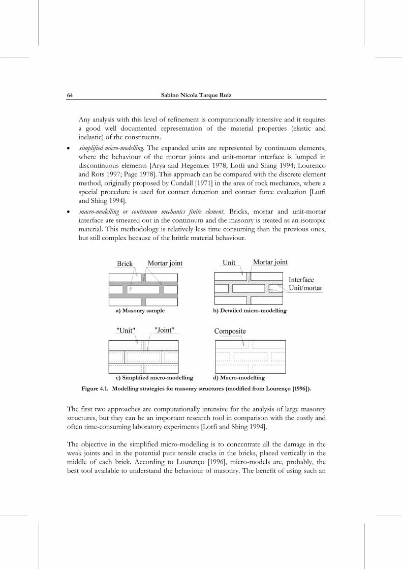
Sabino Nicola Tarque Ruíz
64
Any analysis with this level of refinement is computationally intensive and it requires a good well documented representation of the material properties (elastic and inelastic) of the constituents.
simplified micro-modelling. The expanded units are represented by continuum elements, where the behaviour of the mortar joints and unit-mortar interface is lumped in discontinuous elements [Arya and Hegemier 1978; Lotfi and Shing 1994; Lourenco and Rots 1997; Page 1978]. This approach can be compared with the discrete element method, originally proposed by Cundall [1971] in the area of rock mechanics, where a special procedure is used for contact detection and contact force evaluation [Lotfi and Shing 1994].
macro-modelling or continuum mechanics finite element. Bricks, mortar and unit-mortar interface are smeared out in the continuum and the masonry is treated as an isotropic material. This methodology is relatively less time consuming than the previous ones, but still complex because of the brittle material behaviour.
a) Masonry sample b) Detailed micro-modelling
c) Simplified micro-modelling d) Macro-modelling
Figure 4.1. Modelling strategies for masonry structures (modified from Lourenço [1996]).
The first two approaches are computationally intensive for the analysis of large masonry structures, but they can be an important research tool in comparison with the costly and often time-consuming laboratory experiments [Lotfi and Shing 1994].
The objective in the simplified micro-modelling is to concentrate all the damage in the weak joints and in the potential pure tensile cracks in the bricks, placed vertically in the middle of each brick. According to Lourenço [1996], micro-models are, probably, the best tool available to understand the behaviour of masonry. The benefit of using such an
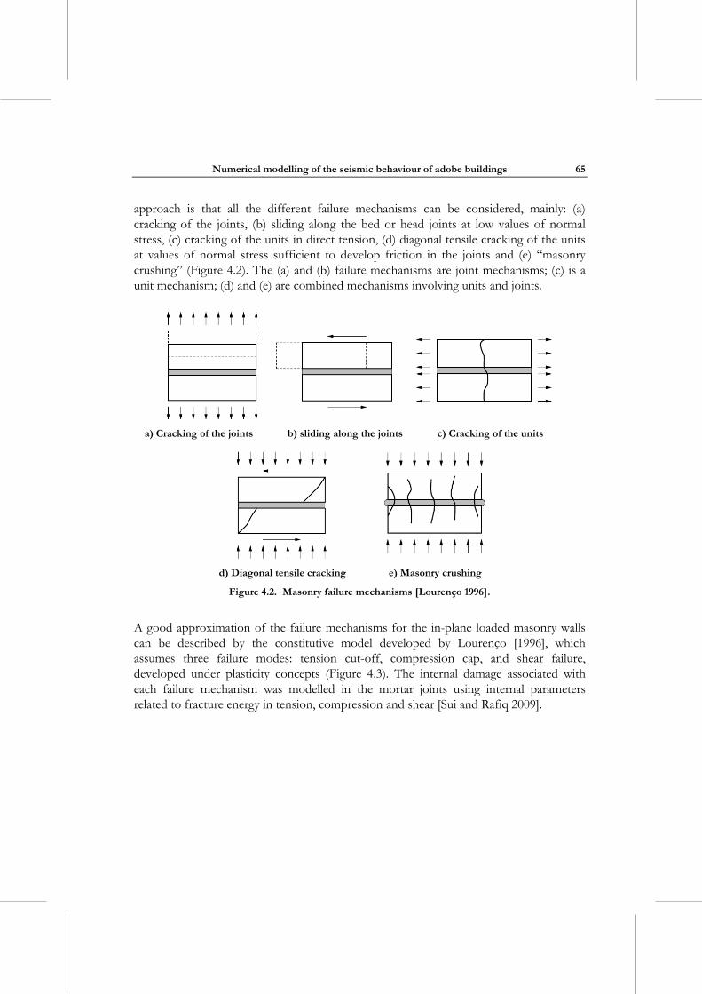
Numerical modelling of the seismic behaviour of adobe buildings
65
approach is that all the different failure mechanisms can be considered, mainly: (a) cracking of the joints, (b) sliding along the bed or head joints at low values of normal stress, (c) cracking of the units in direct tension, (d) diagonal tensile cracking of the units at values of normal stress sufficient to develop friction in the joints and (e) “masonry crushing” (Figure 4.2). The (a) and (b) failure mechanisms are joint mechanisms; (c) is a unit mechanism; (d) and (e) are combined mechanisms involving units and joints.
a) Cracking of the joints b) sliding along the joints c) Cracking of the units
d) Diagonal tensile cracking e) Masonry crushing
Figure 4.2. Masonry failure mechanisms [Lourenço 1996].
A good approximation of the failure mechanisms for the in-plane loaded masonry walls can be described by the constitutive model developed by Lourenço [1996], which assumes three failure modes: tension cut-off, compression cap, and shear failure, developed under plasticity concepts (Figure 4.3). The internal damage associated with each failure mechanism was modelled in the mortar joints using internal parameters related to fracture energy in tension, compression and shear [Sui and Rafiq 2009].
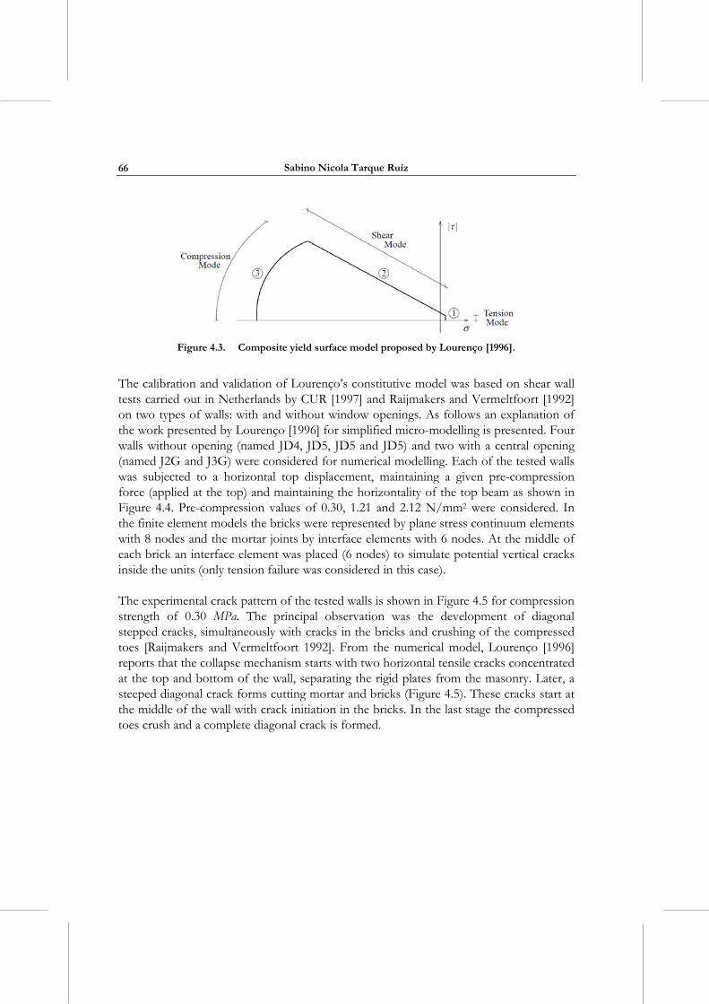
Sabino Nicola Tarque Ruíz
66
Figure 4.3. Composite yield surface model proposed by Lourenço [1996].
The calibration and validation of Lourenço’s constitutive model was based on shear wall tests carried out in Netherlands by CUR [1997] and Raijmakers and Vermeltfoort [1992] on two types of walls: with and without window openings. As follows an explanation of the work presented by Lourenço [1996] for simplified micro-modelling is presented. Four walls without opening (named JD4, JD5, JD5 and JD5) and two with a central opening (named J2G and J3G) were considered for numerical modelling. Each of the tested walls was subjected to a horizontal top displacement, maintaining a given pre-compression force (applied at the top) and maintaining the horizontality of the top beam as shown in Figure 4.4. Pre-compression values of 0.30, 1.21 and 2.12 N/mm2 were considered. In the finite element models the bricks were represented by plane stress continuum elements with 8 nodes and the mortar joints by interface elements with 6 nodes. At the middle of each brick an interface element was placed (6 nodes) to simulate potential vertical cracks inside the units (only tension failure was considered in this case).
The experimental crack pattern of the tested walls is shown in Figure 4.5 for compression strength of 0.30 MPa. The principal observation was the development of diagonal stepped cracks, simultaneously with cracks in the bricks and crushing of the compressed toes [Raijmakers and Vermeltfoort 1992]. From the numerical model, Lourenço [1996] reports that the collapse mechanism starts with two horizontal tensile cracks concentrated at the top and bottom of the wall, separating the rigid plates from the masonry. Later, a steeped diagonal crack forms cutting mortar and bricks (Figure 4.5). These cracks start at the middle of the wall with crack initiation in the bricks. In the last stage the compressed toes crush and a complete diagonal crack is formed.
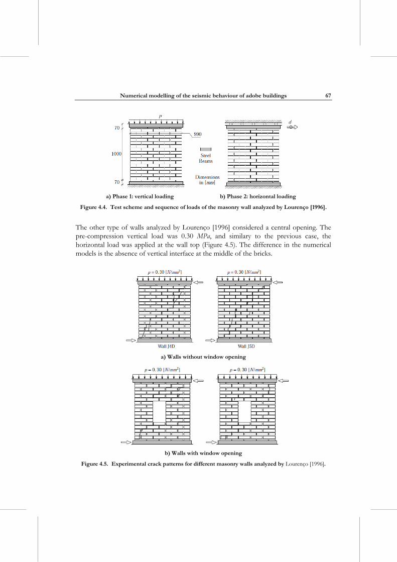
Numerical modelling of the seismic behaviour of adobe buildings
67
a) Phase 1: vertical loading b) Phase 2: horizontal loading
Figure 4.4. Test scheme and sequence of loads of the masonry wall analyzed by Lourenço [1996].
The other type of walls analyzed by Lourenço [1996] considered a central opening. The pre-compression vertical load was 0.30 MPa, and similary to the previous case, the horizontal load was applied at the wall top (Figure 4.5). The difference in the numerical models is the absence of vertical interface at the middle of the bricks.
a) Walls without window opening
b) Walls with window opening
Figure 4.5. Experimental crack patterns for different masonry walls analyzed by Lourenço [1996].
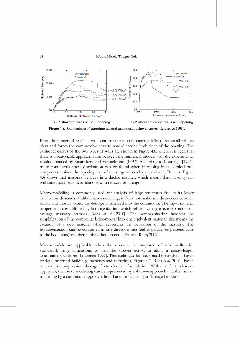
Sabino Nicola Tarque Ruíz
68
a) Pushover of walls without opening b) Pushover curves of walls with opening
Figure 4.6. Comparison of experimental and analytical pushover curves [Lourenço 1996].
From the numerical results it was seen that the central opening defined two small relative piers and forces the compressive strut to spread around both sides of the opening. The pushover curves of the two types of walls are shown in Figure 4.6, where it is seen that there is a reasonable approximation between the numerical models with the experimental results obtained by Raijmakers and Vermeltfoort (1992). According to Lourenço [1996], more continuous stress distribution can be found when increasing initial vertical pre-compression since the opening size of the diagonal cracks are reduced. Besides, Figure 4.6 shows that masonry behaves in a ductile manner, which means that masonry can withstand post-peak deformations with reduced of strength.
Macro-modelling is commonly used for analysis of large structures due to its lower calculation demands. Unlike micro-modelling, it does not make any distinction between bricks and mortar joints, the damage is smeared into the continuum. The input material properties are established by homogenization, which relates average masonry strains and average masonry stresses [Roca et al. 2010]. The homogenization involves the simplification of the composite brick-mortar into one equivalent material; this means the creation of a new material which represents the behaviour of the masonry. The homogenization can be computed in one direction first (either parallel or perpendicular to the bed joints) and then in the other direction [Sui and Rafiq 2009].
Macro-models are applicable when the structure is composed of solid walls with sufficiently large dimensions so that the stresses across or along a macro-length areessentially uniform [Lourenço 1996]. This technique has been used for analysis of arch bridges, historical buildings, mosques and cathedrals, Figure 4.7 [Roca et al. 2010], based on tension-compression damage finite element formulation. Within a finite element approach, the micro-modelling can be represented by a discrete approach and the macro-modelling by a continuum approach; both based on cracking or damaged models.
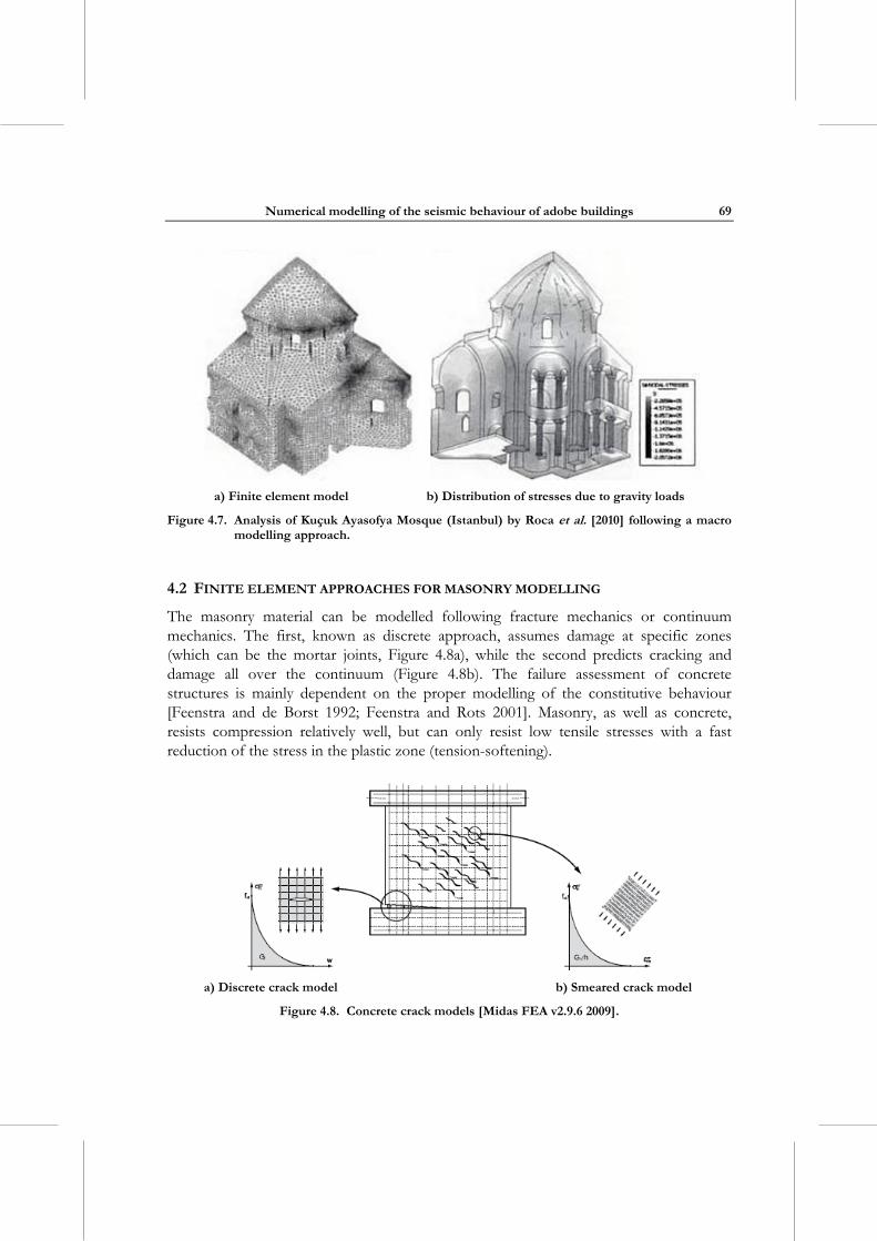
Numerical modelling of the seismic behaviour of adobe buildings
69
a) Finite element model b) Distribution of stresses due to gravity loads
Figure 4.7. Analysis of Kuçuk Ayasofya Mosque (Istanbul) by Roca et al. [2010] following a macro modelling approach.
4.2 FINITE ELEMENT APPROACHES FOR MASONRY MODELLING
The masonry material can be modelled following fracture mechanics or continuum mechanics. The first, known as discrete approach, assumes damage at specific zones (which can be the mortar joints, Figure 4.8a), while the second predicts cracking and damage all over the continuum (Figure 4.8b). The failure assessment of concrete structures is mainly dependent on the proper modelling of the constitutive behaviour [Feenstra and de Borst 1992; Feenstra and Rots 2001]. Masonry, as well as concrete, resists compression relatively well, but can only resist low tensile stresses with a fast reduction of the stress in the plastic zone (tension-softening).
a) Discrete crack model b) Smeared crack model
Figure 4.8. Concrete crack models [Midas FEA v2.9.6 2009].
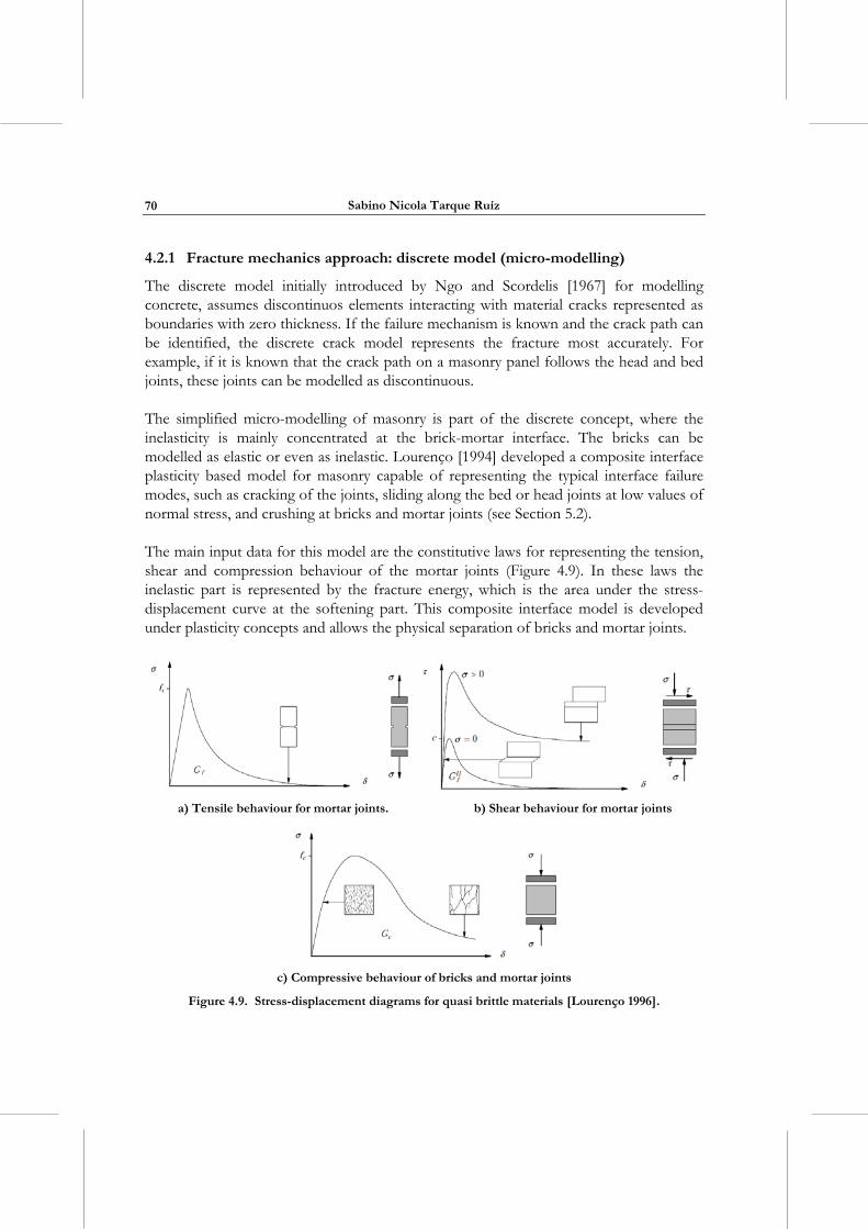
Sabino Nicola Tarque Ruíz
70
4.2.1 Fracture mechanics approach: discrete model (micro-modelling)
The discrete model initially introduced by Ngo and Scordelis [1967] for modelling concrete, assumes discontinuos elements interacting with material cracks represented as boundaries with zero thickness. If the failure mechanism is known and the crack path can be identified, the discrete crack model represents the fracture most accurately. For example, if it is known that the crack path on a masonry panel follows the head and bed joints, these joints can be modelled as discontinuous.
The simplified micro-modelling of masonry is part of the discrete concept, where the inelasticity is mainly concentrated at the brick-mortar interface. The bricks can be modelled as elastic or even as inelastic. Lourenço [1994] developed a composite interface plasticity based model for masonry capable of representing the typical interface failure modes, such as cracking of the joints, sliding along the bed or head joints at low values of normal stress, and crushing at bricks and mortar joints (see Section 5.2).
The main input data for this model are the constitutive laws for representing the tension, shear and compression behaviour of the mortar joints (Figure 4.9). In these laws the inelastic part is represented by the fracture energy, which is the area under the stress-displacement curve at the softening part. This composite interface model is developed under plasticity concepts and allows the physical separation of bricks and mortar joints.
a) Tensile behaviour for mortar joints. b) Shear behaviour for mortar joints
c) Compressive behaviour of bricks and mortar joints
Figure 4.9. Stress-displacement diagrams for quasi brittle materials [Lourenço 1996].
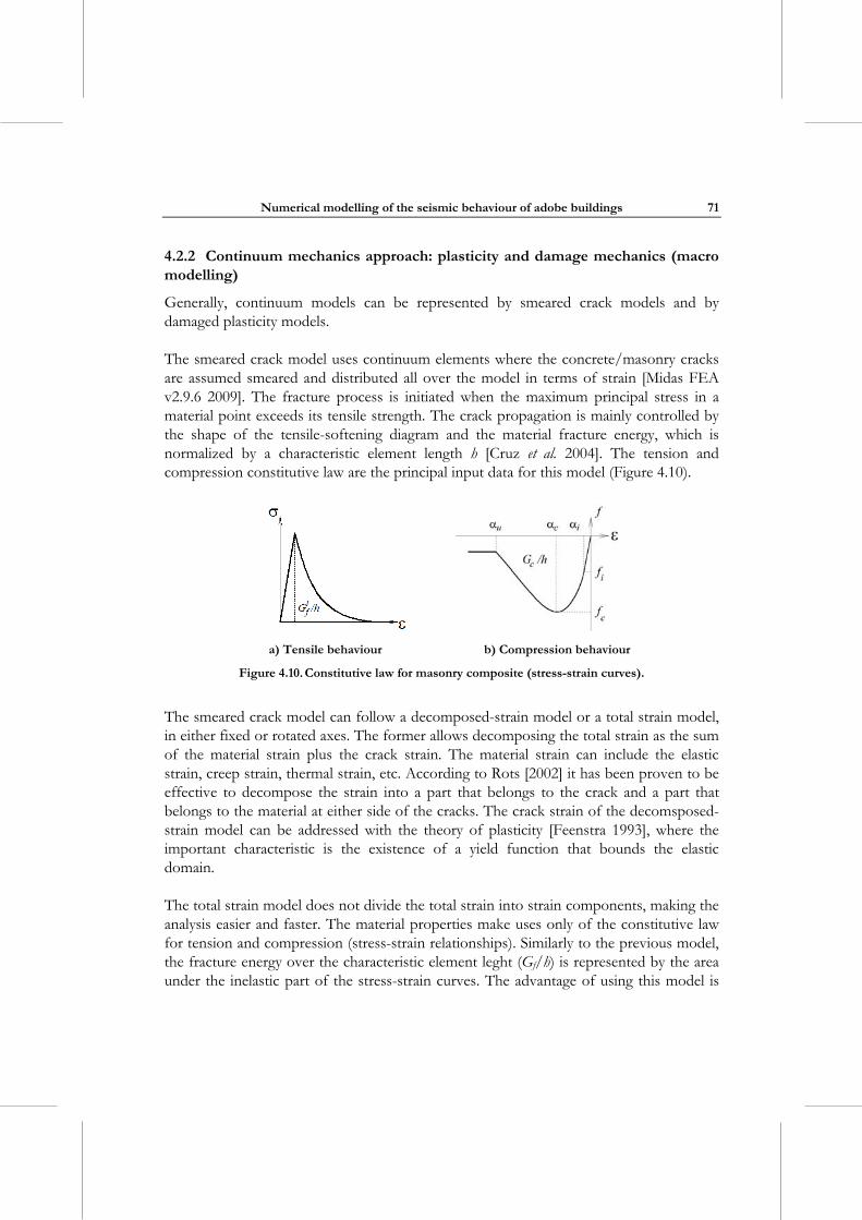
Numerical modelling of the seismic behaviour of adobe buildings
71
4.2.2 Continuum mechanics approach: plasticity and damage mechanics (macro modelling)
Generally, continuum models can be represented by smeared crack models and by damaged plasticity models.
The smeared crack model uses continuum elements where the concrete/masonry cracks are assumed smeared and distributed all over the model in terms of strain [Midas FEA v2.9.6 2009]. The fracture process is initiated when the maximum principal stress in a material point exceeds its tensile strength. The crack propagation is mainly controlled by the shape of the tensile-softening diagram and the material fracture energy, which is normalized by a characteristic element length h [Cruz et al. 2004]. The tension and compression constitutive law are the principal input data for this model (Figure 4.10).
a) Tensile behaviour b) Compression behaviour
Figure 4.10. Constitutive law for masonry composite (stress-strain curves).
The smeared crack model can follow a decomposed-strain model or a total strain model, in either fixed or rotated axes. The former allows decomposing the total strain as the sum of the material strain plus the crack strain. The material strain can include the elastic strain, creep strain, thermal strain, etc. According to Rots [2002] it has been proven to be effective to decompose the strain into a part that belongs to the crack and a part that belongs to the material at either side of the cracks. The crack strain of the decomsposed-strain model can be addressed with the theory of plasticity [Feenstra 1993], where the important characteristic is the existence of a yield function that bounds the elastic domain.
The total strain model does not divide the total strain into strain components, making the analysis easier and faster. The material properties make uses only of the constitutive law for tension and compression (stress-strain relationships). Similarly to the previous model, the fracture energy over the characteristic element leght (Gf/h) is represented by the area under the inelastic part of the stress-strain curves. The advantage of using this model is
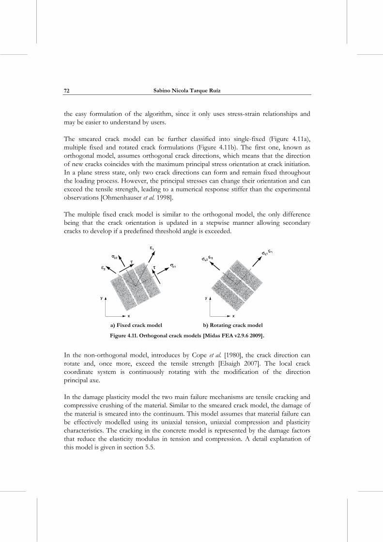
Sabino Nicola Tarque Ruíz
72
the easy formulation of the algorithm, since it only uses stress-strain relationships and may be easier to understand by users.
The smeared crack model can be further classified into single-fixed (Figure 4.11a), multiple fixed and rotated crack formulations (Figure 4.11b). The first one, known as orthogonal model, assumes orthogonal crack directions, which means that the direction of new cracks coincides with the maximum principal stress orientation at crack initiation. In a plane stress state, only two crack directions can form and remain fixed throughout the loading process. However, the principal stresses can change their orientation and can exceed the tensile strength, leading to a numerical response stiffer than the experimental observations [Ohmenhauser et al. 1998].
The multiple fixed crack model is similar to the orthogonal model, the only difference being that the crack orientation is updated in a stepwise manner allowing secondary cracks to develop if a predefined threshold angle is exceeded.
a) Fixed crack model b) Rotating crack model
Figure 4.11. Orthogonal crack models [Midas FEA v2.9.6 2009].
In the non-orthogonal model, introduces by Cope et al. [1980], the crack direction can rotate and, once more, exceed the tensile strength [Elsaigh 2007]. The local crack coordinate system is continuously rotating with the modification of the direction principal axe.
In the damage plasticity model the two main failure mechanisms are tensile cracking and compressive crushing of the material. Similar to the smeared crack model, the damage of the material is smeared into the continuum. This model assumes that material failure can be effectively modelled using its uniaxial tension, uniaxial compression and plasticity characteristics. The cracking in the concrete model is represented by the damage factors that reduce the elasticity modulus in tension and compression. A detail explanation of this model is given in section 5.5.
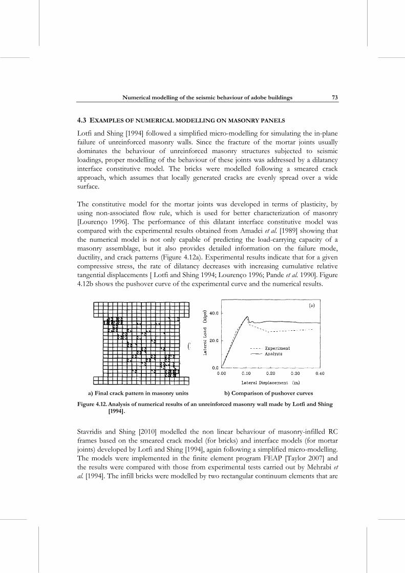
Numerical modelling of the seismic behaviour of adobe buildings
73
4.3 EXAMPLES OF NUMERICAL MODELLING ON MASONRY PANELS
Lotfi and Shing [1994] followed a simplified micro-modelling for simulating the in-plane failure of unreinforced masonry walls. Since the fracture of the mortar joints usually dominates the behaviour of unreinforced masonry structures subjected to seismic loadings, proper modelling of the behaviour of these joints was addressed by a dilatancy interface constitutive model. The bricks were modelled following a smeared crack approach, which assumes that locally generated cracks are evenly spread over a wide surface.
The constitutive model for the mortar joints was developed in terms of plasticity, by using non-associated flow rule, which is used for better characterization of masonry [Lourenço 1996]. The performance of this dilatant interface constitutive model was compared with the experimental results obtained from Amadei et al. [1989] showing that the numerical model is not only capable of predicting the load-carrying capacity of a masonry assemblage, but it also provides detailed information on the failure mode, ductility, and crack patterns (Figure 4.12a). Experimental results indicate that for a given compressive stress, the rate of dilatancy decreases with increasing cumulative relative tangential displacements [ Lotfi and Shing 1994; Lourenço 1996; Pande et al. 1990]. Figure 4.12b shows the pushover curve of the experimental curve and the numerical results.
a) Final crack pattern in masonry units b) Comparison of pushover curves
Figure 4.12. Analysis of numerical results of an unreinforced masonry wall made by Lotfi and Shing [1994].
Stavridis and Shing [2010] modelled the non linear behaviour of masonry-infilled RC frames based on the smeared crack model (for bricks) and interface models (for mortar joints) developed by Lotfi and Shing [1994], again following a simplified micro-modelling. The models were implemented in the finite element program FEAP [Taylor 2007] and the results were compared with those from experimental tests carried out by Mehrabi et al. [1994]. The infill bricks were modelled by two rectangular continuum elements that are
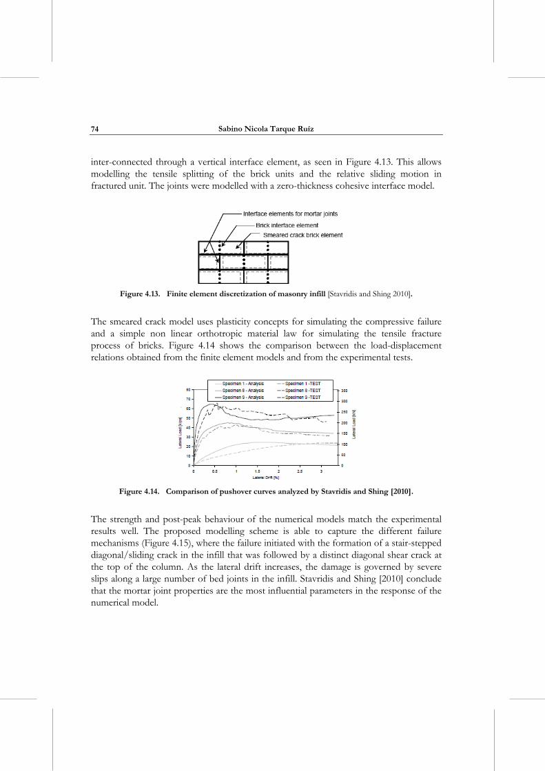
Sabino Nicola Tarque Ruíz
74
inter-connected through a vertical interface element, as seen in Figure 4.13. This allows modelling the tensile splitting of the brick units and the relative sliding motion in fractured unit. The joints were modelled with a zero-thickness cohesive interface model.
Figure 4.13. Finite element discretization of masonry infill [Stavridis and Shing 2010].
The smeared crack model uses plasticity concepts for simulating the compressive failure and a simple non linear orthotropic material law for simulating the tensile fracture process of bricks. Figure 4.14 shows the comparison between the load-displacement relations obtained from the finite element models and from the experimental tests.
Figure 4.14. Comparison of pushover curves analyzed by Stavridis and Shing [2010].
The strength and post-peak behaviour of the numerical models match the experimental results well. The proposed modelling scheme is able to capture the different failure mechanisms (Figure 4.15), where the failure initiated with the formation of a stair-stepped diagonal/sliding crack in the infill that was followed by a distinct diagonal shear crack at the top of the column. As the lateral drift increases, the damage is governed by severe slips along a large number of bed joints in the infill. Stavridis and Shing [2010] conclude that the mortar joint properties are the most influential parameters in the response of the numerical model.
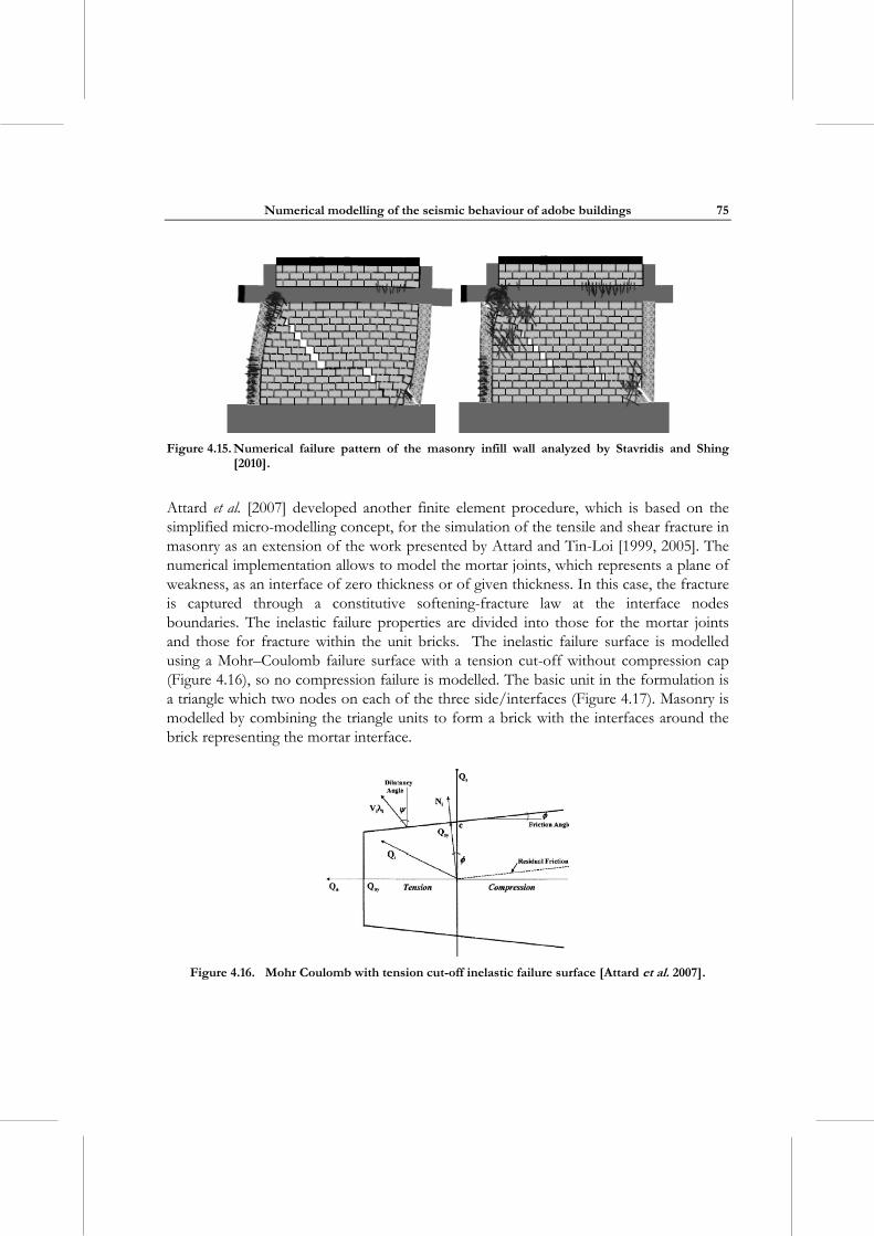
Numerical modelling of the seismic behaviour of adobe buildings
75
Figure 4.15. Numerical failure pattern of the masonry infill wall analyzed by Stavridis and Shing
[2010].
Attard et al. [2007] developed another finite element procedure, which is based on the simplified micro-modelling concept, for the simulation of the tensile and shear fracture in masonry as an extension of the work presented by Attard and Tin-Loi [1999, 2005]. The numerical implementation allows to model the mortar joints, which represents a plane of weakness, as an interface of zero thickness or of given thickness. In this case, the fracture is captured through a constitutive softening-fracture law at the interface nodes boundaries. The inelastic failure properties are divided into those for the mortar joints and those for fracture within the unit bricks. The inelastic failure surface is modelled using a Mohr–Coulomb failure surface with a tension cut-off without compression cap (Figure 4.16), so no compression failure is modelled. The basic unit in the formulation is a triangle which two nodes on each of the three side/interfaces (Figure 4.17). Masonry is modelled by combining the triangle units to form a brick with the interfaces around the brick representing the mortar interface.
Figure 4.16. Mohr Coulomb with tension cut-off inelastic failure surface [Attard et al. 2007].
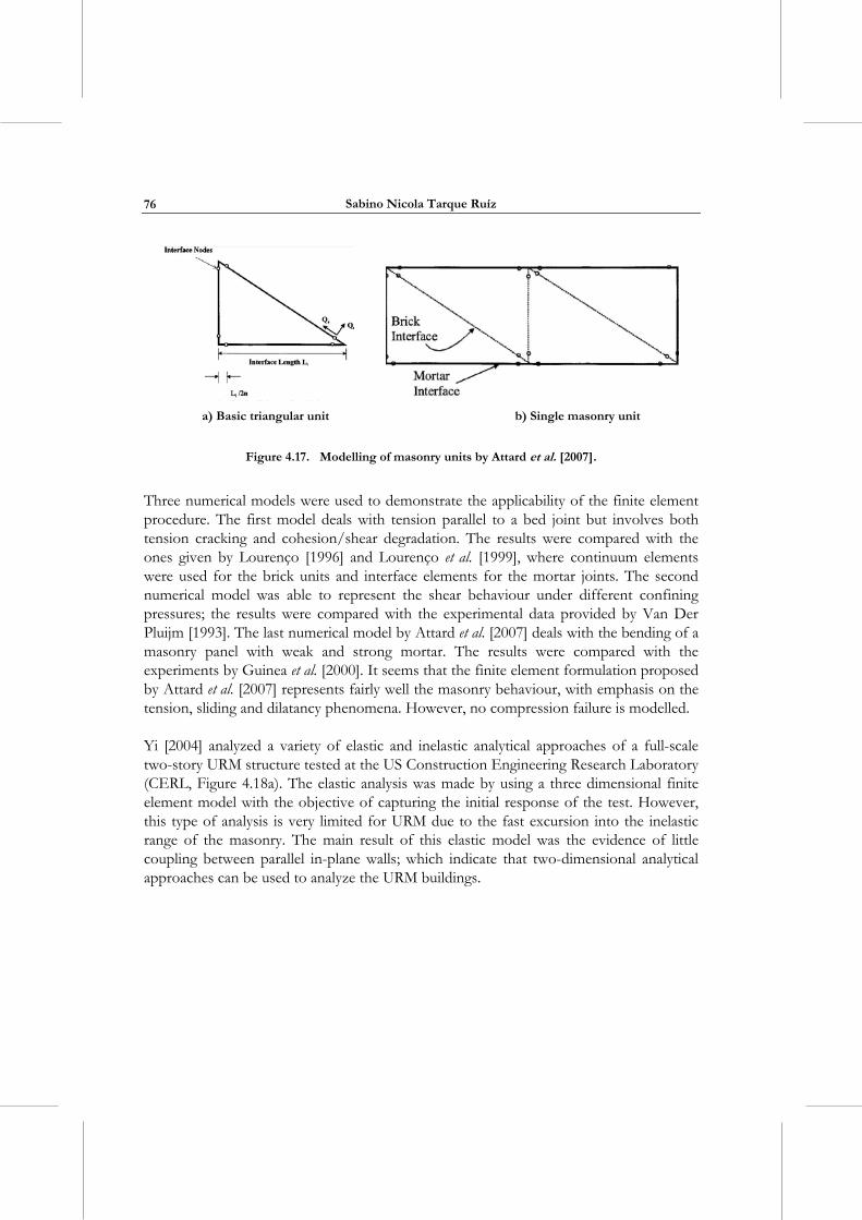
Sabino Nicola Tarque Ruíz
76
a) Basic triangular unit b) Single masonry unit
Figure 4.17. Modelling of masonry units by Attard et al. [2007].
Three numerical models were used to demonstrate the applicability of the finite element procedure. The first model deals with tension parallel to a bed joint but involves both tension cracking and cohesion/shear degradation. The results were compared with the ones given by Lourenço [1996] and Lourenço et al. [1999], where continuum elements were used for the brick units and interface elements for the mortar joints. The second numerical model was able to represent the shear behaviour under different confining pressures; the results were compared with the experimental data provided by Van Der Pluijm [1993]. The last numerical model by Attard et al. [2007] deals with the bending of a masonry panel with weak and strong mortar. The results were compared with the experiments by Guinea et al. [2000]. It seems that the finite element formulation proposed by Attard et al. [2007] represents fairly well the masonry behaviour, with emphasis on the tension, sliding and dilatancy phenomena. However, no compression failure is modelled.
Yi [2004] analyzed a variety of elastic and inelastic analytical approaches of a full-scale two-story URM structure tested at the US Construction Engineering Research Laboratory (CERL, Figure 4.18a). The elastic analysis was made by using a three dimensional finite element model with the objective of capturing the initial response of the test. However, this type of analysis is very limited for URM due to the fast excursion into the inelastic range of the masonry. The main result of this elastic model was the evidence of little coupling between parallel in-plane walls; which indicate that two-dimensional analytical approaches can be used to analyze the URM buildings.
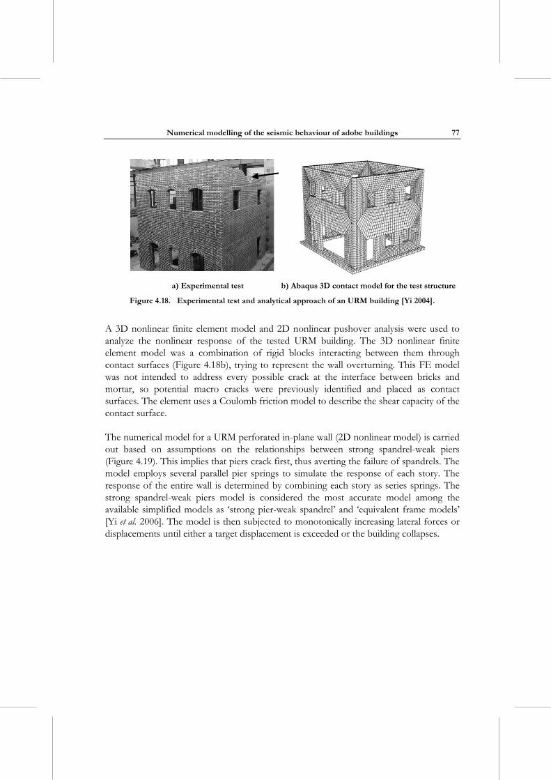
Numerical modelling of the seismic behaviour of adobe buildings
77
a) Experimental test b) Abaqus 3D contact model for the test structure
Figure 4.18. Experimental test and analytical approach of an URM building [Yi 2004].
A 3D nonlinear finite element model and 2D nonlinear pushover analysis were used to analyze the nonlinear response of the tested URM building. The 3D nonlinear finite element model was a combination of rigid blocks interacting between them through contact surfaces (Figure 4.18b), trying to represent the wall overturning. This FE model was not intended to address every possible crack at the interface between bricks and mortar, so potential macro cracks were previously identified and placed as contact surfaces. The element uses a Coulomb friction model to describe the shear capacity of the contact surface.
The numerical model for a URM perforated in-plane wall (2D nonlinear model) is carried out based on assumptions on the relationships between strong spandrel-weak piers (Figure 4.19). This implies that piers crack first, thus averting the failure of spandrels. The model employs several parallel pier springs to simulate the response of each story. The response of the entire wall is determined by combining each story as series springs. The strong spandrel-weak piers model is considered the most accurate model among the available simplified models as ‘strong pier-weak spandrel’ and ‘equivalent frame models’ [Yi et al. 2006]. The model is then subjected to monotonically increasing lateral forces or displacements until either a target displacement is exceeded or the building collapses.
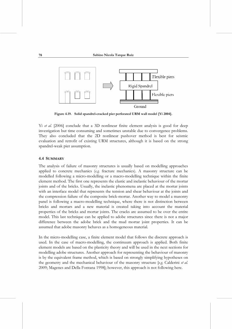
Sabino Nicola Tarque Ruíz
78
Figure 4.19. Solid spandrel-cracked pier perforated URM wall model [Yi 2004].
Yi et al. [2006] conclude that a 3D nonlinear finite element analysis is good for deep investigation but time consuming and sometimes unstable due to convergence problems. They also concluded that the 2D nonlinear pushover method is best for seismic evaluation and retrofit of existing URM structures, although it is based on the strong spandrel-weak pier assumption.
4.4 SUMMARY
The analysis of failure of masonry structures is usually based on modelling approaches applied to concrete mechanics (e.g. fracture mechanics). A masonry structure can be modelled following a micro-modelling or a macro-modelling technique within the finite element method. The first one represents the elastic and inelastic behaviour of the mortar joints and of the bricks. Usually, the inelastic phenomena are placed at the mortar joints with an interface model that represents the tension and shear behaviour at the joints and the compression failure of the composite brick-mortar. Another way to model a masonry panel is following a macro-modelling technique, where there is not distinction between bricks and mortars and a new material is created taking into account the material properties of the bricks and mortar joints. The cracks are assumed to be over the entire model. This last technique can be applied to adobe structures since there is not a major difference between the adobe brick and the mud mortar joint properties. It can be assumed that adobe masonry behaves as a homogeneous material.
In the micro-modelling case, a finite element model that follows the discrete approach is used. In the case of macro-modelling, the continuum approach is applied. Both finite element models are based on the plasticity theory and will be used in the next sections for modelling adobe structures. Another approach for representing the behaviour of masonry is by the equivalent frame method, which is based on strongly simplifying hypotheses on the geometry and the mechanical behaviour of the masonry structure [e.g. Calderini et al. 2009; Magenes and Della Fontana 1998]; however, this approach is not following here.
Numerical modelling of the seismic behaviour of adobe buildings
79
5. DISCRETE AND CONTINUUM MODELS FOR REPRESENTING THE SEISMIC BEHAVIOUR OF MASONRY
The material behaviour of a model (body) can be reproduced through a Finite Element idealization making use of stress-strain relationships (constitutive models) that represents the stress state in a material point of the body. Specifically for quasi brittle materials, the material cracking can be modelled using two general approaches: discrete and continuum. These approaches have been studied by many authors [e.g. Lotfi and Shing 1994; Ngo and Scordelis 1967; Rots 1991] and also applied to masonry structures. This chapter describes the concepts of each approach and its mathematical formulation, with details on the application to masonry structures.
5.1 REVIEW OF THEORY OF PLASTICITY
Plasticity is a tool for describing ductile material behaviours. Plasticity describes materials, such as ductile metals, clay or putty, which allows bodies to change their shape by the application of forces, and retain their new shape upon removal of such forces [Lubliner 2006]. This means that materials exhibit permanent or irreversible deformations also after unloading. Tipically plastic materials are metals, but plasticity is extended to brittle materials because of its computational advantages. Materials such as soils, rock and concrete, can be defined as plastic materials with great sensitivity to pressure, resulting in very different strengths in tension and compression.
The important characteristic in the plasticity theory is the existence of a yield function that bounds the elastic domain. The essential elements of any constitutive model based on the classical plasticity theory are the yield criterion, which determine if the material responds purely elastically at a particular state of stress; the flow rule, which defines the inelastic deformation that occurs if the material point is no longer responding elastically; and the hardening rule, which defines the way in which the yield and flow rule change as inelastic deformation occurs [Koiter 1960].
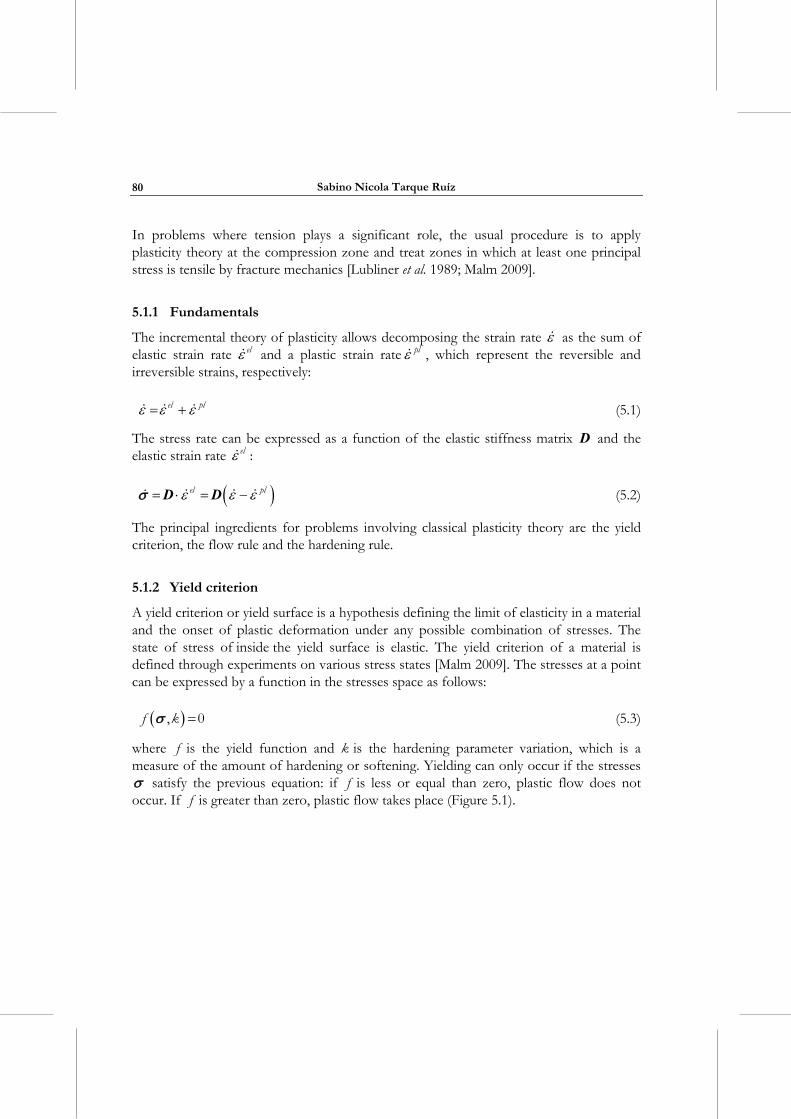
Sabino Nicola Tarque Ruíz
80
In problems where tension plays a significant role, the usual procedure is to apply plasticity theory at the compression zone and treat zones in which at least one principal stress is tensile by fracture mechanics [Lubliner et al. 1989; Malm 2009].
5.1.1 Fundamentals
The incremental theory of plasticity allows decomposing the strain rate as the sum of elastic strain rate el and a plastic strain rate pl , which represent the reversible and irreversible strains, respectively:
el pl (5.1)
The stress rate can be expressed as a function of the elastic stiffness matrix D and the elastic strain rate el :
el pl D D (5.2)
The principal ingredients for problems involving classical plasticity theory are the yield criterion, the flow rule and the hardening rule.
5.1.2 Yield criterion
A yield criterion or yield surface is a hypothesis defining the limit of elasticity in a material and the onset of plastic deformation under any possible combination of stresses. The state of stress of inside the yield surface is elastic. The yield criterion of a material is defined through experiments on various stress states [Malm 2009]. The stresses at a point can be expressed by a function in the stresses space as follows:
f k, 0 (5.3)
where f is the yield function and k is the hardening parameter variation, which is a measure of the amount of hardening or softening. Yielding can only occur if the stresses satisfy the previous equation: if f is less or equal than zero, plastic flow does not occur. If f is greater than zero, plastic flow takes place (Figure 5.1).
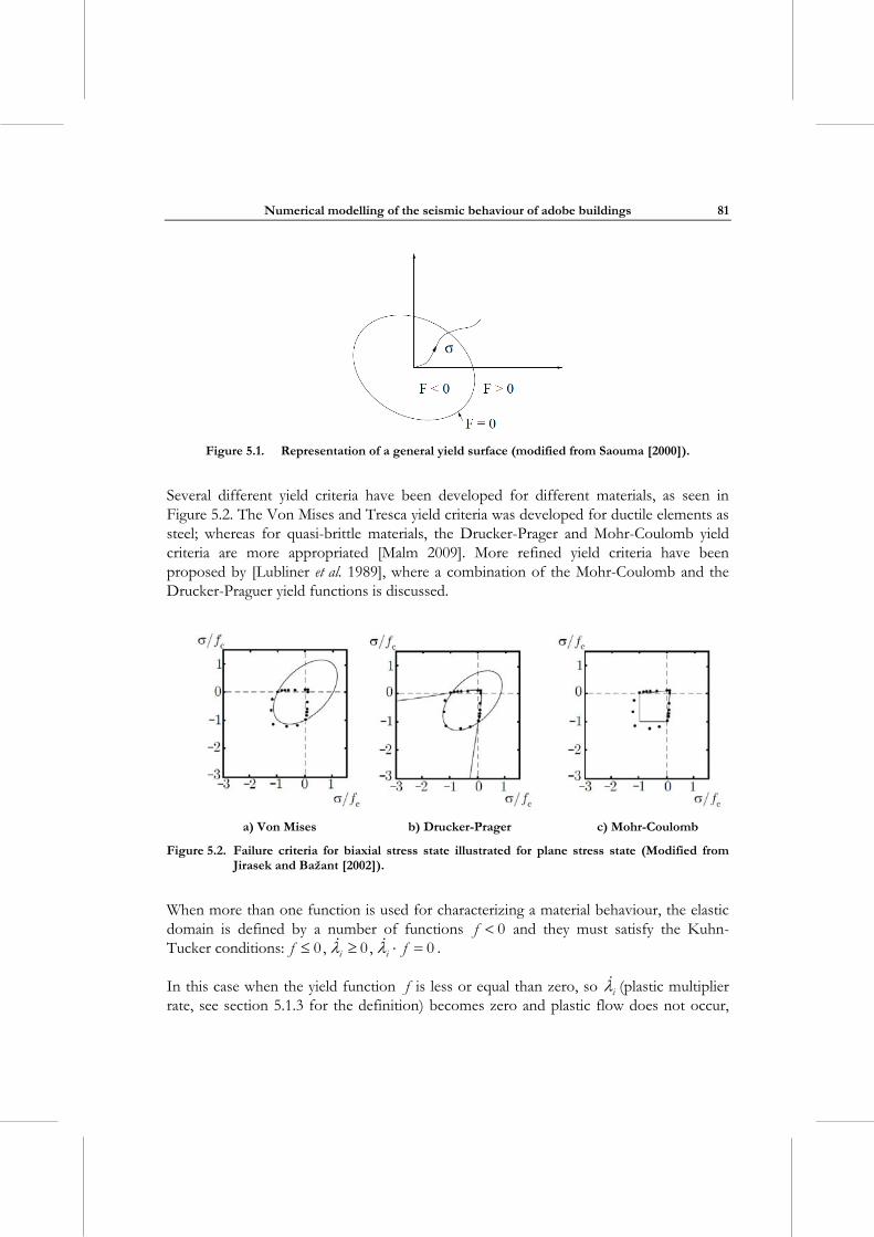
Numerical modelling of the seismic behaviour of adobe buildings
81
Figure 5.1. Representation of a general yield surface (modified from Saouma [2000]).
Several different yield criteria have been developed for different materials, as seen in Figure 5.2. The Von Mises and Tresca yield criteria was developed for ductile elements as steel; whereas for quasi-brittle materials, the Drucker-Prager and Mohr-Coulomb yield criteria are more appropriated [Malm 2009]. More refined yield criteria have been proposed by [Lubliner et al. 1989], where a combination of the Mohr-Coulomb and the Drucker-Praguer yield functions is discussed.
a) Von Mises b) Drucker-Prager c) Mohr-Coulomb
Figure 5.2. Failure criteria for biaxial stress state illustrated for plane stress state (Modified from Jirasek and Bažant [2002]).
When more than one function is used for characterizing a material behaviour, the elastic domain is defined by a number of functions f 0 and they must satisfy the Kuhn-Tucker conditions: i if f0 , 0 , 0 .
In this case when the yield function f is less or equal than zero, so i (plastic multiplier rate, see section 5.1.3 for the definition) becomes zero and plastic flow does not occur,
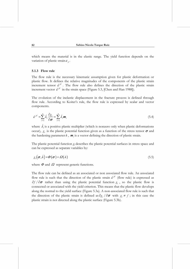
Sabino Nicola Tarque Ruíz
82
which means the material is in the elastic range. The yield function depends on the variation of plastic strain p .
5.1.3 Flow rule
The flow rule is the necessary kinematic assumption given for plastic deformation or plastic flow. It defines the relative magnitudes of the components of the plastic strain increment tensor pl . The flow rule also defines the direction of the plastic strain increment vector pl in the strain space (Figure 5.3, [Chen and Han 1988]).
The evolution of the inelastic displacement in the fracture process is defined through flow rule. According to Koiter’s rule, the flow rule is expressed by scalar and vector components.
n npl i
i i ii i
g
1 1
m
(5.4)
where i is a positive plastic multiplier (which is nonzero only when plastic deformations occur), ig is the plastic potential function given as a function of the stress tensor and the hardening parameter k , im is a vector defining the direction of plastic strain.
The plastic potential function gi describes the plastic potential surfaces in stress space and can be expressed as separate variables by:
ig k k, (5.5)
where and represent generic functions.
The flow rule can be defined as an associated or non associated flow rule. An associated flow rule is such that the direction of the plastic strain pl (flow rule) is expressed as
f / rather than using the plastic potential function ig , so the plastic flow is connected or associated with the yield criterion. This means that the plastic flow develops along the normal to the yield surface (Figure 5.3a). A non-associated flow rule is such that the direction of the plastic strain is defined as ig / with ig f ; in this case the plastic strain is not directed along the plastic surface (Figure 5.3b).
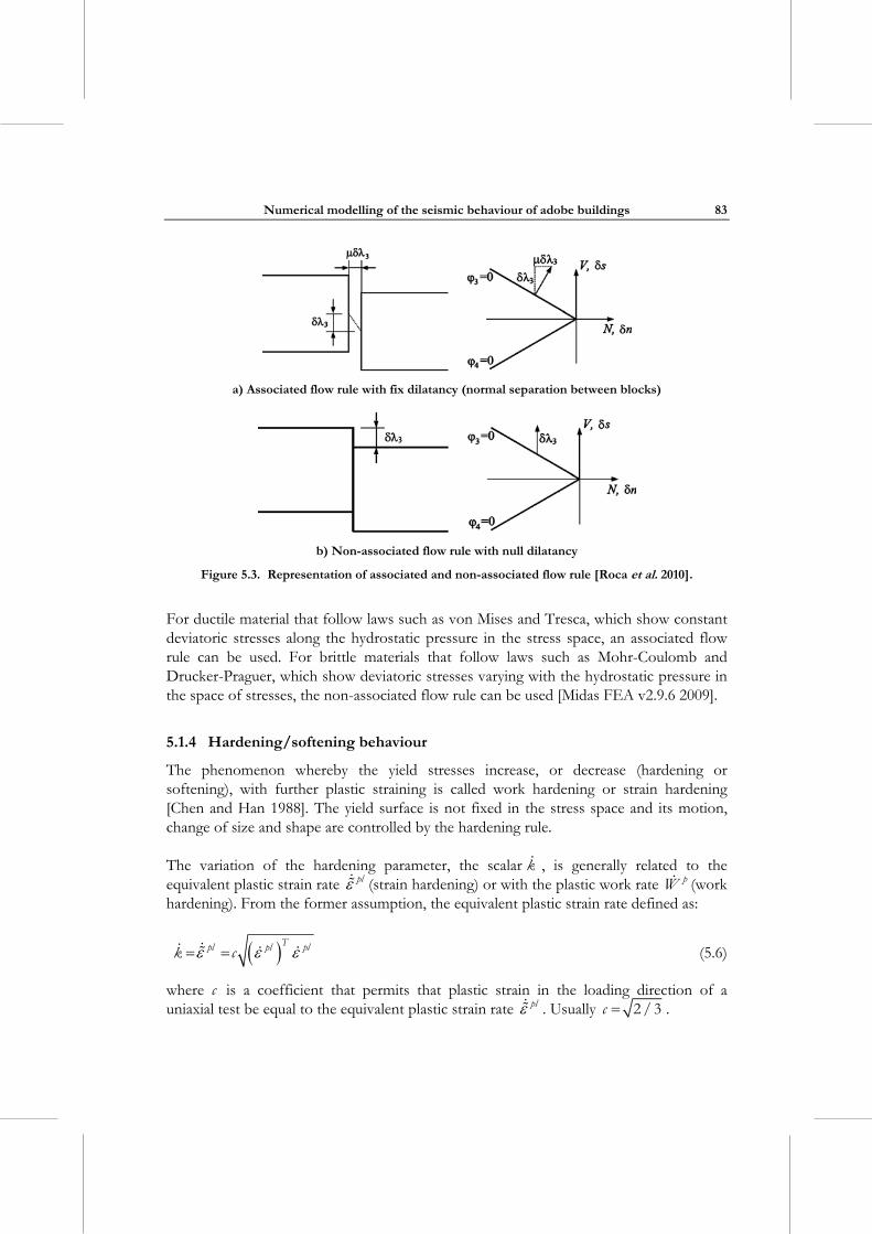
Numerical modelling of the seismic behaviour of adobe buildings
83
a) Associated flow rule with fix dilatancy (normal separation between blocks)
b) Non-associated flow rule with null dilatancy
Figure 5.3. Representation of associated and non-associated flow rule [Roca et al. 2010].
For ductile material that follow laws such as von Mises and Tresca, which show constant deviatoric stresses along the hydrostatic pressure in the stress space, an associated flow rule can be used. For brittle materials that follow laws such as Mohr-Coulomb and Drucker-Praguer, which show deviatoric stresses varying with the hydrostatic pressure in the space of stresses, the non-associated flow rule can be used [Midas FEA v2.9.6 2009].
5.1.4 Hardening/softening behaviour
The phenomenon whereby the yield stresses increase, or decrease (hardening or softening), with further plastic straining is called work hardening or strain hardening [Chen and Han 1988]. The yield surface is not fixed in the stress space and its motion, change of size and shape are controlled by the hardening rule.
The variation of the hardening parameter, the scalar k , is generally related to the equivalent plastic strain rate pl (strain hardening) or with the plastic work rate pW (work hardening). From the former assumption, the equivalent plastic strain rate defined as:
Tpl pl plk c (5.6)
where c is a coefficient that permits that plastic strain in the loading direction of a uniaxial test be equal to the equivalent plastic strain rate pl . Usually c 2 / 3 .
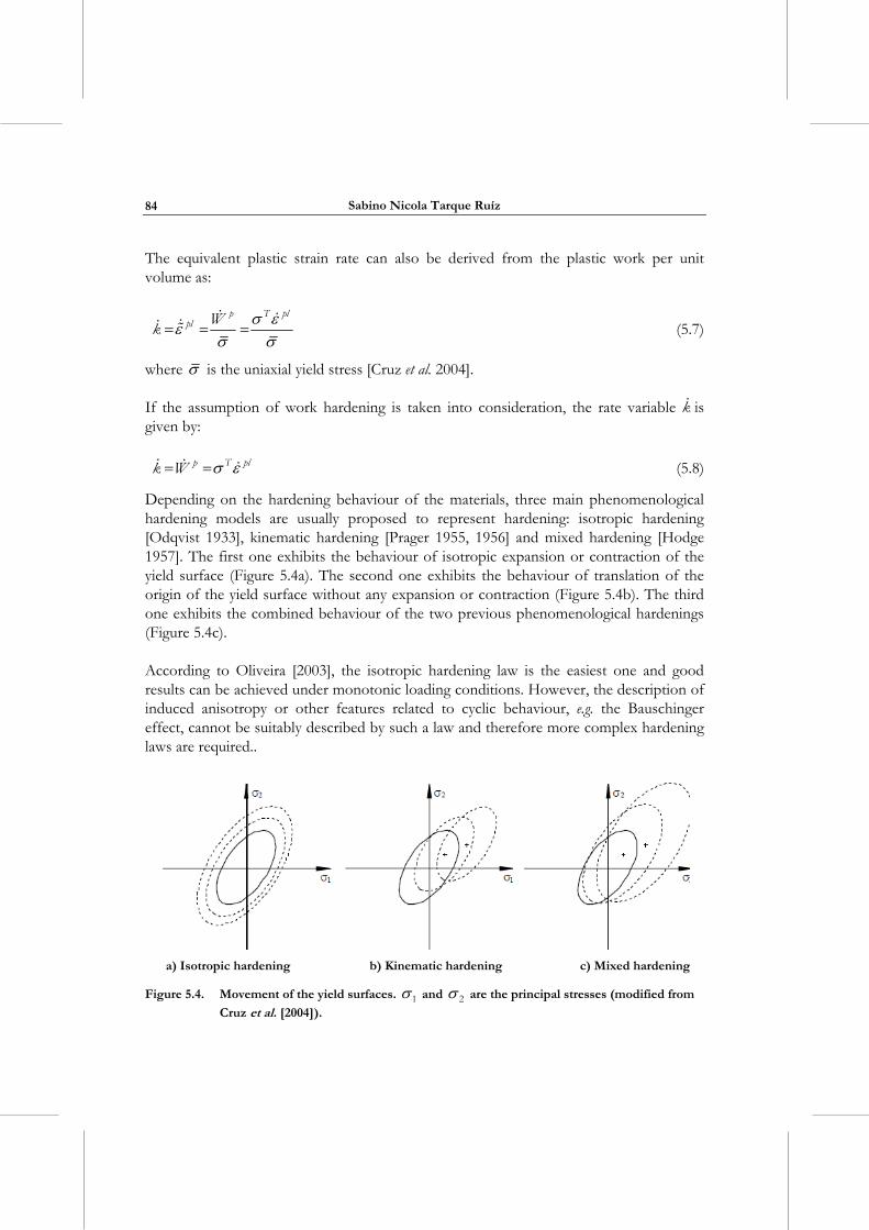
Sabino Nicola Tarque Ruíz
84
The equivalent plastic strain rate can also be derived from the plastic work per unit volume as:
p T plpl W
k
(5.7)
where is the uniaxial yield stress [Cruz et al. 2004].
If the assumption of work hardening is taken into consideration, the rate variable k is given by:
p T plk W (5.8)
Depending on the hardening behaviour of the materials, three main phenomenological hardening models are usually proposed to represent hardening: isotropic hardening [Odqvist 1933], kinematic hardening [Prager 1955, 1956] and mixed hardening [Hodge 1957]. The first one exhibits the behaviour of isotropic expansion or contraction of the yield surface (Figure 5.4a). The second one exhibits the behaviour of translation of the origin of the yield surface without any expansion or contraction (Figure 5.4b). The third one exhibits the combined behaviour of the two previous phenomenological hardenings (Figure 5.4c).
According to Oliveira [2003], the isotropic hardening law is the easiest one and good results can be achieved under monotonic loading conditions. However, the description of induced anisotropy or other features related to cyclic behaviour, e.g. the Bauschinger effect, cannot be suitably described by such a law and therefore more complex hardening laws are required..
a) Isotropic hardening b) Kinematic hardening c) Mixed hardening
Figure 5.4. Movement of the yield surfaces. 1 and 2 are the principal stresses (modified from
Cruz et al. [2004]).
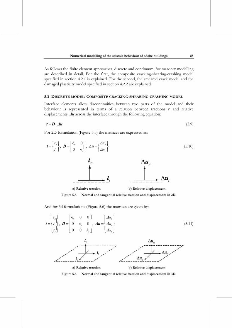
Numerical modelling of the seismic behaviour of adobe buildings
85
As follows the finite element approaches, discrete and continuum, for masonry modelling are described in detail. For the first, the composite cracking-shearing-crashing model specified in section 4.2.1 is explained. For the second, the smeared crack model and the damaged plasticity model specified in section 4.2.2 are explained.
5.2 DISCRETE MODEL: COMPOSITE CRACKING-SHEARING-CRASHING MODEL
Interface elements allow discontinuities between two parts of the model and their behaviour is represented in terms of a relation between tractions t and relative displacements u across the interface through the following equation:
t D u (5.9)
For 2D formulation (Figure 5.5) the matrices are expressed as:
n n n
s s s
t k u
t k u
0, ,
0
t D u (5.10)
a) Relative traction b) Relative displacement
Figure 5.5. Normal and tangential relative traction and displacement in 2D.
And for 3d formulations (Figure 5.6) the matrices are given by:
n n n
s s s
t t t
t k u
t k u
t k u
0 0
, 0 0 ,
0 0
t D u (5.11)
a) Relative traction b) Relative displacement
Figure 5.6. Normal and tangential relative traction and displacement in 3D.
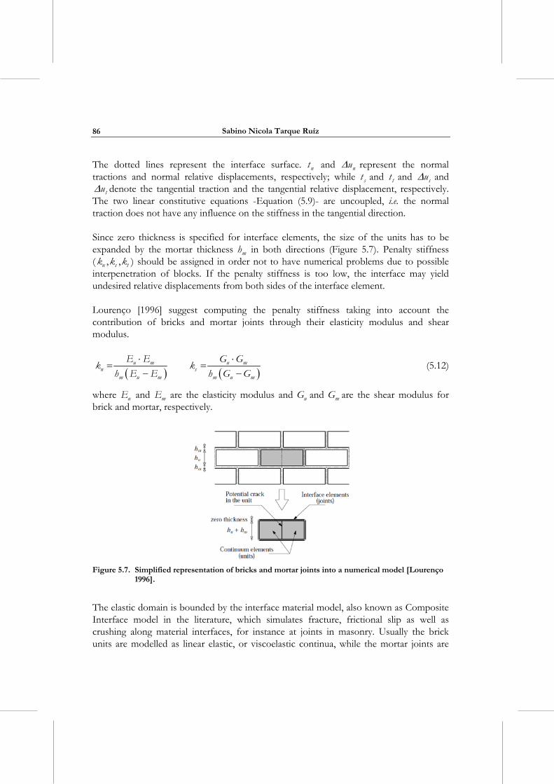
Sabino Nicola Tarque Ruíz
86
The dotted lines represent the interface surface. nt and nu represent the normal tractions and normal relative displacements, respectively; while st and tt and su and
tu denote the tangential traction and the tangential relative displacement, respectively. The two linear constitutive equations -Equation (5.9)- are uncoupled, i.e. the normal traction does not have any influence on the stiffness in the tangential direction.
Since zero thickness is specified for interface elements, the size of the units has to be expanded by the mortar thickness mh in both directions (Figure 5.7). Penalty stiffness ( n s tk k k, , ) should be assigned in order not to have numerical problems due to possible interpenetration of blocks. If the penalty stiffness is too low, the interface may yield undesired relative displacements from both sides of the interface element.
Lourenço [1996] suggest computing the penalty stiffness taking into account the contribution of bricks and mortar joints through their elasticity modulus and shear modulus.
u m u m
n sm u m m u m
E E G Gk k
h E E h G G
(5.12)
where uE and mE are the elasticity modulus and uG and mG are the shear modulus for brick and mortar, respectively.
Figure 5.7. Simplified representation of bricks and mortar joints into a numerical model [Lourenço
1996].
The elastic domain is bounded by the interface material model, also known as Composite Interface model in the literature, which simulates fracture, frictional slip as well as crushing along material interfaces, for instance at joints in masonry. Usually the brick units are modelled as linear elastic, or viscoelastic continua, while the mortar joints are
Numerical modelling of the seismic behaviour of adobe buildings
87
modelled with interface elements, which obey the nonlinear behaviour described by the composite interface model (also known as combined cracking–shearing–crushing model. The law to characterize the inelasticity behaviour is given in terms of plasticity.
Lourenço [1996] used a simplified micro-modelling procedure for analysis of masonry walls, basically for in-plane mechanical behaviour. In this case the inelasticity was concentrated at the interface elements (usually the mortar joints) where crack, slip or crushing can occur. If it is necessary, the inelasticity is also located in the middle of bricks to represent potential pure tensile cracks (Figure 5.7).
This composite interface model is a combination of three plastic surfaces that represent tension, shear and compression failure. A tension cut-off it is considered for tension failure. For the shear failure, the softening process is given by the degradation of the cohesion in Coulomb friction models. For the compression failure, Lourenço [1996] developed a suitable cap model. Each of the failure mechanisms is associated with a hardening/softening rule for representing the inelasticity at any material point. Since the masonry joints have extremely low dilatancy (almost zero, [Lourenço 1996]), the model was formulated in the context of non-associated plasticity.
The principal input data for the composite interface model are the constitutive laws for representing the tension, shear and compression behaviour of the mortar joints. In these laws the inelastic part is represented by the fracture energy, which is the area under the stress-displacement curve at the softening part (inelastic part). The softening is a gradual decrease of the mechanical strength under a continuous increase of deformation. This behaviour is attributed to the heterogeneity of the material, due to the presence of different phases and material defects, such as flaws and voids, and also due to micro-cracks due to shrinkage during curing and the presence of the aggregate [Lourenço 1998].
5.2.1 Two-dimensional interface model
The interface model is derived in terms of generalized stress and strain vectors as follows:
u
v,
(5.13)
where σ and u are the stress and relative displacement in the normal direction of the interface, and τ and ν are the shear stress and relative displacement respectively.
In the elastic range, the constitutive behaviour is described by:
D (5.14)
Sabino Nicola Tarque Ruíz
88
with the stiffness matrix explained before: n sdiag k kD
5.2.1.1 Shear-slipping
The shear-slipping criterion is defined by the following Coulomb friction yield/crack criterion:
f c (5.15)
where is the shear stress, Ф is the friction coefficient equal to the friction angle tan , c is the cohesion of the brick-mortar interface. An exponential softening function is assumed for the cohesion. For the friction angle, the softening is taken proportional to the softening of the cohesion. The cohesion softening is defined as follows:
IIf
cc k c k
G0
0, exp
(5.16)
where c0 is the initial cohesion of the brick-mortar interface, IIfG is the shear slip fracture
energy, k is the hardening parameter.
The friction softening is coupled to the cohesion softening by:
rc c
kc
00 0
0
, (5.17)
where 0 and r are the initial and the residual friction coefficients, respectively.
The mode II fracture energy, IIfG , increases under increasing confining pressure as seen
in experimental results by Van Der Pluijm [1993]. The experimentally observed linear relation between the fracture energy and the normal confining stress is defined as:
IIf
a b ifG
b if
0
0
(5.18)
Where a and b are constants determined by linear regression of the experimental data.
Dilatancy
The non-associated flow rule is expressed as follows:
Numerical modelling of the seismic behaviour of adobe buildings
89
p
p
u gv
pε
(5.19)
The plastic potential function for describing the dilatancy is given by:
g
sign
(5.20)
where tan is the mobilized dilatancy coefficient. From Equations (5.19) and (5.20) the following equation is obtained:
p
p
usign
v
(5.21)
By integration, the shear-slip induced normal uplift is found to be:
p pu d v (5.22)
The dilatancy is considered as a function of the plastic relative shear displacement and the normal confining pressure. Under increasing value of these two quantities, the dilatancy angle tends to zero. The dilatancy formulation, Equation(5.23), can be expressed as separate values to simplify curve fitting and to ensure convexity of the potential function g:
pv1 2 (5.23)
T
pg
g d v d2 1 (5.24)
Therefore, a description of the normal uplift upon shear-slipping is:
u
p p uu
p
if
u v if
v if
0
0
0
1 1 exp 0
1 exp 0
(5.25)
which yields after differentiation in
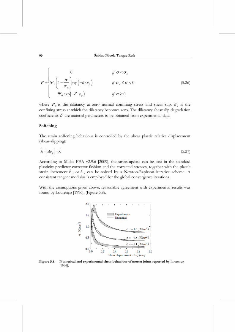
Sabino Nicola Tarque Ruíz
90
u
p uu
p
if
v if
v if
0
0
0
1 exp 0
exp 0
(5.26)
where 0 is the dilatancy at zero normal confining stress and shear slip. u is the confining stress at which the dilatancy becomes zero. The dilatancy shear slip degradation coefficients are material parameters to be obtained from experimental data.
Softening
The strain softening behaviour is controlled by the shear plastic relative displacement (shear-slipping):
pk v (5.27)
According to Midas FEA v2.9.6 [2009], the stress-update can be cast in the standard plasticity predictor-corrector fashion and the corrected stresses, together with the plastic strain increment k , or , can be solved by a Newton-Raphson iterative scheme. A consistent tangent modulus is employed for the global convergence iterations.
With the assumptions given above, reasonable agreement with experimental results was found by Lourenço [1996], (Figure 5.8).
Figure 5.8. Numerical and experimental shear behaviour of mortar joints reported by Lourenço
[1996].
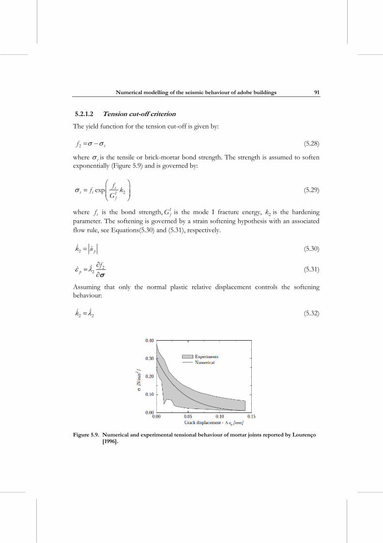
Numerical modelling of the seismic behaviour of adobe buildings
91
5.2.1.2 Tension cut-off criterion
The yield function for the tension cut-off is given by:
tf 2 (5.28)
where t is the tensile or brick-mortar bond strength. The strength is assumed to soften exponentially (Figure 5.9) and is governed by:
tt t I
f
ff k
G 2exp
(5.29)
where tf is the bond strength, IfG is the mode I fracture energy, k2 is the hardening
parameter. The softening is governed by a strain softening hypothesis with an associated flow rule, see Equations(5.30) and (5.31), respectively.
pk u2 (5.30)
pf 2
2
(5.31)
Assuming that only the normal plastic relative displacement controls the softening behaviour:
k2 2 (5.32)
Figure 5.9. Numerical and experimental tensional behaviour of mortar joints reported by Lourenço
[1996].
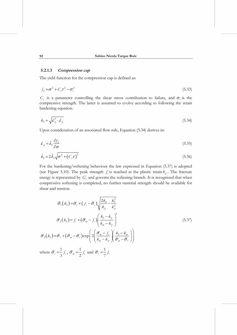
Sabino Nicola Tarque Ruíz
92
5.2.1.3 Compression cap
The yield function for the compression cap is defined as:
s cf C2 2 23 (5.33)
sC is a parameter controlling the shear stress contribution to failure, and c is the compressive strength. The latter is assumed to evolve according to following the strain hardening equation.
Tp pk3 (5.34)
Upon consideration of an associated flow rule, Equation (5.34) derives in:
p
f33
(5.35)
sk C22
3 32 (5.36)
For the hardening/softening behaviour the law expressed in Equation (5.37) is adopted (see Figure 5.10). The peak strength cf is reached at the plastic strain pk . The fracture energy is represented by c
fG and governs the softening branch. It is recognized that when compressive softening is completed, no further material strength should be available for shear and tension.
i c ip p
pc m c
m p
m c mr m r
m p m r
k kk f
k k
k kk f f
k k
f k kk
k k
23 3
1 3 2
2
32 3
33 3
2
exp 2
(5.37)
where i cf1
3 , m cf
1
2 and r cf
1
7
Numerical modelling of the seismic behaviour of adobe buildings
93
Figure 5.10. Hardening/softening compression law for masonry [Lourenço 1996].
Corners
At each of the intersections of the Coulomb friction criterion with the tension cut-off and the compression cap, the plastic strain increment is given by:
ip i
gg11
(5.38)
Subscript 1 refers to shear criterion and i, which can be 2 or 3, refers to tension cut-off or compression cap, respectively. In both the shear/tension corner and the shear/compression corner, the stress corrections can be written in a standard predictor-corrector fashion and solved with the two plastic strain increments 1 or i with a Newton-Raphson scheme [Lourenço 1996].
5.2.2 Three-dimensional interface model
The 3D yield function, without considering the compression cap model, is shown in Figure 5.11 [Midas FEA v2.9.6 2009]. The generalized stress and strain vectors are shown in the following equation:
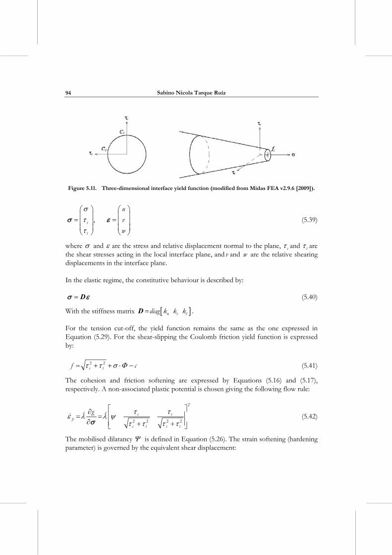
Sabino Nicola Tarque Ruíz
94
Figure 5.11. Three-dimensional interface yield function (modified from Midas FEA v2.9.6 [2009]).
s
t
u
v
w
,
(5.39)
where and are the stress and relative displacement normal to the plane, s and t are the shear stresses acting in the local interface plane, and v and w are the relative shearing displacements in the interface plane.
In the elastic regime, the constitutive behaviour is described by:
D (5.40)
With the stiffness matrix n s tdiag k k kD .
For the tension cut-off, the yield function remains the same as the one expressed in Equation (5.29). For the shear-slipping the Coulomb friction yield function is expressed by:
s tf c2 2 (5.41)
The cohesion and friction softening are expressed by Equations (5.16) and (5.17), respectively. A non-associated plastic potential is chosen giving the following flow rule:
T
s tp
s t s t
g2 2 2 2
(5.42)
The mobilised dilatancy is defined in Equation (5.26). The strain softening (hardening parameter) is governed by the equivalent shear displacement:
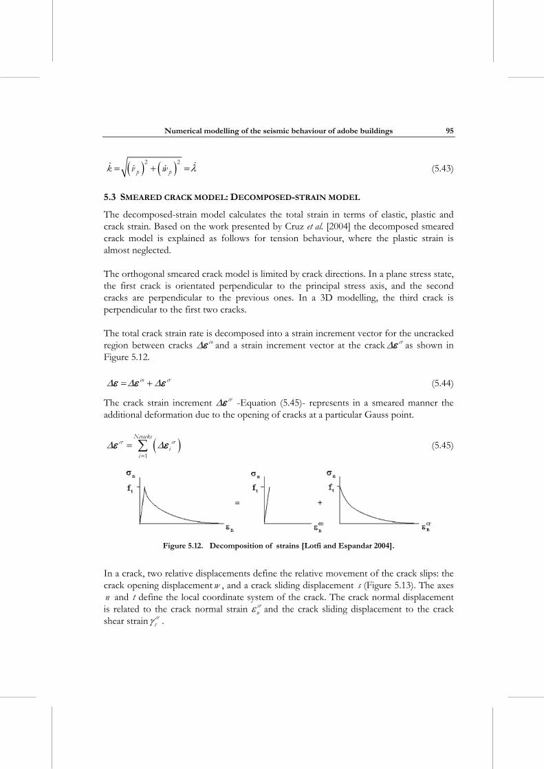
Numerical modelling of the seismic behaviour of adobe buildings
95
p pk v w2 2
(5.43)
5.3 SMEARED CRACK MODEL: DECOMPOSED-STRAIN MODEL
The decomposed-strain model calculates the total strain in terms of elastic, plastic and crack strain. Based on the work presented by Cruz et al. [2004] the decomposed smeared crack model is explained as follows for tension behaviour, where the plastic strain is almost neglected.
The orthogonal smeared crack model is limited by crack directions. In a plane stress state, the first crack is orientated perpendicular to the principal stress axis, and the second cracks are perpendicular to the previous ones. In a 3D modelling, the third crack is perpendicular to the first two cracks.
The total crack strain rate is decomposed into a strain increment vector for the uncracked region between cracks co and a strain increment vector at the crack cr as shown in Figure 5.12.
co cr (5.44)
The crack strain increment cr -Equation (5.45)- represents in a smeared manner the additional deformation due to the opening of cracks at a particular Gauss point.
Ncracks
cr cri
i 1
(5.45)
Figure 5.12. Decomposition of strains [Lotfi and Espandar 2004].
In a crack, two relative displacements define the relative movement of the crack slips: the crack opening displacement w , and a crack sliding displacement s (Figure 5.13). The axes n and t define the local coordinate system of the crack. The crack normal displacement is related to the crack normal strain cr
n and the crack sliding displacement to the crack shear strain cr
t .
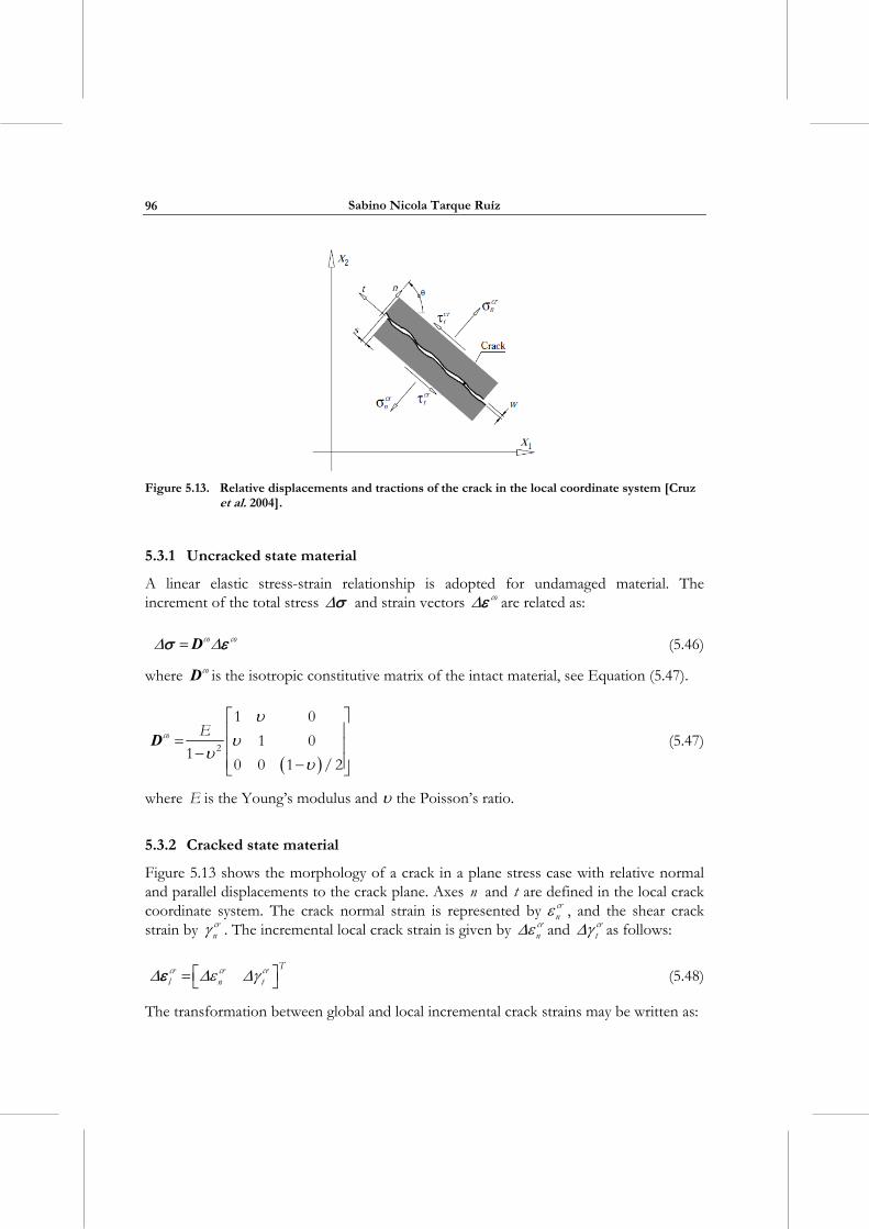
Sabino Nicola Tarque Ruíz
96
Figure 5.13. Relative displacements and tractions of the crack in the local coordinate system [Cruz
et al. 2004].
5.3.1 Uncracked state material
A linear elastic stress-strain relationship is adopted for undamaged material. The increment of the total stress and strain vectors co are related as:
co co D (5.46)
where coD is the isotropic constitutive matrix of the intact material, see Equation (5.47).
co E2
1 0
1 01
0 0 1 / 2
D (5.47)
where E is the Young’s modulus and the Poisson’s ratio.
5.3.2 Cracked state material
Figure 5.13 shows the morphology of a crack in a plane stress case with relative normal and parallel displacements to the crack plane. Axes n and t are defined in the local crack coordinate system. The crack normal strain is represented by cr
n , and the shear crack strain by cr
n . The incremental local crack strain is given by crn and cr
t as follows:
Tcr cr crl n t (5.48)
The transformation between global and local incremental crack strains may be written as:
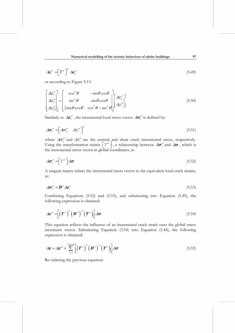
Numerical modelling of the seismic behaviour of adobe buildings
97
Tcr cr crl T (5.49)
or according to Figure 5.13:
cr
crncr
crtcr
21
22
2 212
cos sin cos
sin sin cos
2sin cos cos sin
(5.50)
Similarly to crl , the incremental local stress vector cr
l is defined by:
Tcr cr crl n t (5.51)
where crn and cr
t are the normal and shear crack incremental stress, respectively. Using the transformation matrix crT , a relationship between cr
l and , which is the incremental stress vector in global coordinates, is:
cr crl T (5.52)
A tangent matrix relates the incremental stress vector to the equivalent local crack strains, as:
cr cr crl l D (5.53)
Combining Equations (5.52) and (5.53), and substituting into Equation (5.49), the following expression is obtained:
Tcr cr cr cr1
T D T (5.54)
This equation reflects the influence of an incremental crack strain onto the global stress increment vector. Substituting Equation (5.54) into Equation (5.44), the following expression is obtained:
Ncrack Tco cr cr cr
i
1
1
T D T (5.55)
Re-ordering the previous equation:
Sabino Nicola Tarque Ruíz
98
Ncrack Tco cr cr cr
i
11 1
1
D T D T (5.56)
or
crco D (5.57)
where crcoD is the constitutive matrix for the cracked material state:
Ncrack Tcrco co cr cr cr
i
11 1
1
D D T D T (5.58)
5.3.3 Crack fracture parameters
The crack constitutive matrix crD distinguishes between mode I and mode II failure and it is assumed that there is no interaction between these two modes. This means that coupling among normal and shear components in the crack traction-strain expressions are neglected [Lotfi and Espandar 2004]. The crD matrix is defined diagonal as:
crIcr
crII
D
D
0
0
D (5.59)
where crID and cr
IID are the mode I and mode II stiffness modulus associated with the crack behaviour.
Mode I stiffness is given by:
cr tI I
f
f hD
G
22
2
(5.60)
where ft is the tensile strength, IfG is the fracture energy release rate, which are material
constants, 2 is a parameter that depends on the shape of the softening curve [Lotfi and Espandar 2004], h is the characteristic length related to mesh size [Bažant and Oh 1983]. When using a 4-nodes shell element, h is taken as the square root of the area of the finite element. For 8-node element, h is half of the previous value. When using a solid, h is the diagonal of the volume.
To avoid snap-back instability, the characteristic length is subjected to the following constraint [de Borst 1991]:
Numerical modelling of the seismic behaviour of adobe buildings
99
f c
t
G Eh
b f 2
(5.61)
where b depends to the shape of the softening curve.
The crack interface shear stiffness crIID is expressed in terms of uncracked material shear
modulus G as:
cr tII
t
D G1
(5.62)
where t is the shear retention factor. A value of 0.1 is suggested by Lotfi and Espandar [2004]. According to Rots [1988], t can be written as:
pcrn
t crn ult
1
,
1
(5.63)
5.4 SMEARED CRACK MODEL: TOTAL-STRAIN MODEL
In this model the stress is assumed to be a function of the total strain [Feenstra and Rots 2001]. This model is divided in a fixed orthogonal crack model or a coaxial rotating crack model, depending on the approach to the shear stress-strain relation. The constitutive relationships can be described in terms of the tension and compression stress-strain relations. When the material enters in the inelastic region, the cracking only influences the diagonal terms in the compliance matrix cD , as specified by Feenstra and de Borst [1992]. In the local coordinate system the total stress-strain relation in plane-stress is:
n t n
n t n t
c c c cn t tl l l
n t n t
t
E E
E E
G
2 2
2 2
01 1
01 1
0 0
D (5.64)
where n and t are reduction factors for the elasticity modulus and are only functions of the tensile strains in the considered directions, t is the shear retention factor. In the global coordinate system the previous equation is re-written using the strain transformation matrix cT that is equal to crT , resulting in:
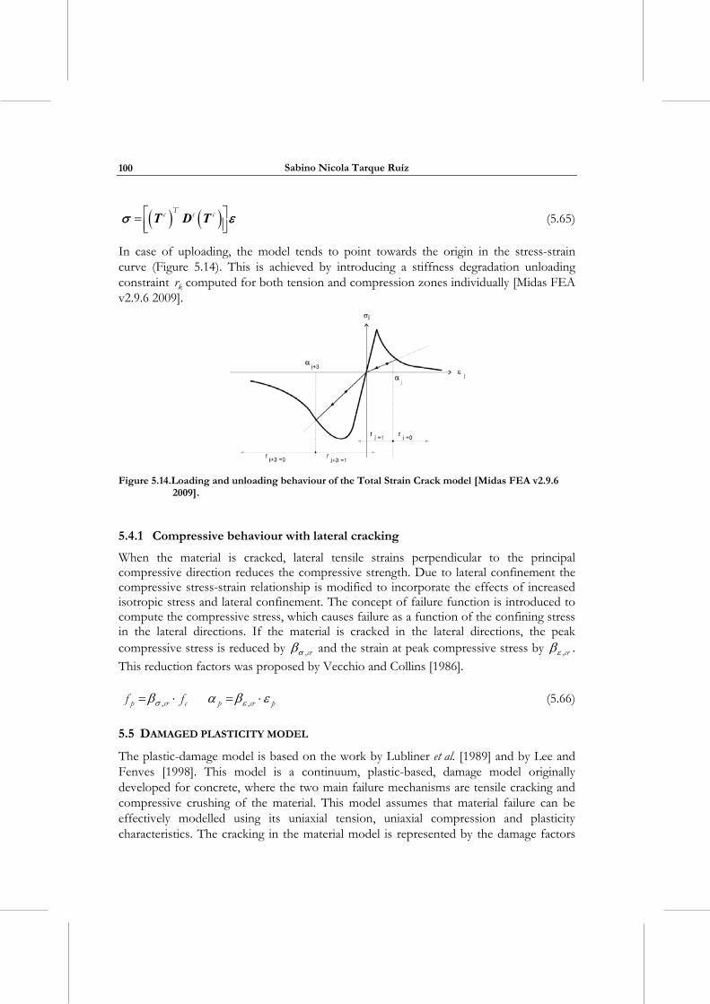
Sabino Nicola Tarque Ruíz
100
Tc c c T D T (5.65)
In case of uploading, the model tends to point towards the origin in the stress-strain curve (Figure 5.14). This is achieved by introducing a stiffness degradation unloading constraint kr computed for both tension and compression zones individually [Midas FEA v2.9.6 2009].
Figure 5.14.Loading and unloading behaviour of the Total Strain Crack model [Midas FEA v2.9.6
2009].
5.4.1 Compressive behaviour with lateral cracking
When the material is cracked, lateral tensile strains perpendicular to the principal compressive direction reduces the compressive strength. Due to lateral confinement the compressive stress-strain relationship is modified to incorporate the effects of increased isotropic stress and lateral confinement. The concept of failure function is introduced to compute the compressive stress, which causes failure as a function of the confining stress in the lateral directions. If the material is cracked in the lateral directions, the peak compressive stress is reduced by cr, and the strain at peak compressive stress by cr, .
This reduction factors was proposed by Vecchio and Collins [1986].
p cr cf f, p cr p, (5.66)
5.5 DAMAGED PLASTICITY MODEL
The plastic-damage model is based on the work by Lubliner et al. [1989] and by Lee and Fenves [1998]. This model is a continuum, plastic-based, damage model originally developed for concrete, where the two main failure mechanisms are tensile cracking and compressive crushing of the material. This model assumes that material failure can be effectively modelled using its uniaxial tension, uniaxial compression and plasticity characteristics. The cracking in the material model is represented by the damage factors
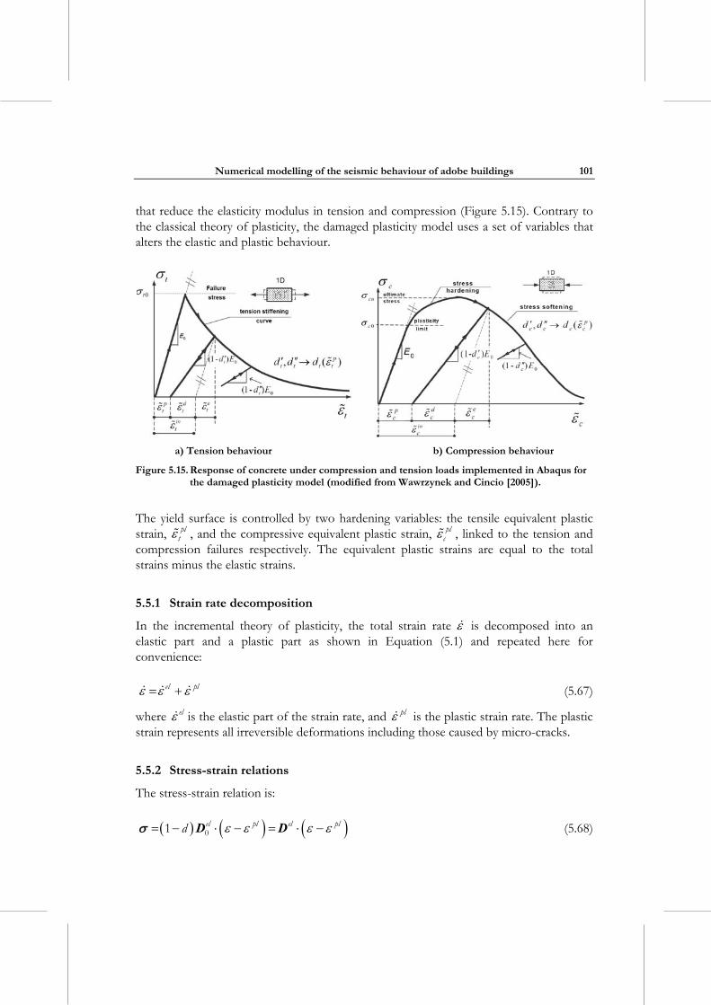
Numerical modelling of the seismic behaviour of adobe buildings
101
that reduce the elasticity modulus in tension and compression (Figure 5.15). Contrary to the classical theory of plasticity, the damaged plasticity model uses a set of variables that alters the elastic and plastic behaviour.
a) Tension behaviour b) Compression behaviour
Figure 5.15. Response of concrete under compression and tension loads implemented in Abaqus for the damaged plasticity model (modified from Wawrzynek and Cincio [2005]).
The yield surface is controlled by two hardening variables: the tensile equivalent plastic strain, pl
t , and the compressive equivalent plastic strain, plc , linked to the tension and
compression failures respectively. The equivalent plastic strains are equal to the total strains minus the elastic strains.
5.5.1 Strain rate decomposition
In the incremental theory of plasticity, the total strain rate is decomposed into an elastic part and a plastic part as shown in Equation (5.1) and repeated here for convenience:
el pl (5.67)
where el is the elastic part of the strain rate, and pl is the plastic strain rate. The plastic strain represents all irreversible deformations including those caused by micro-cracks.
5.5.2 Stress-strain relations
The stress-strain relation is:
el pl el pld 01 D D (5.68)
Sabino Nicola Tarque Ruíz
102
where el0D is the undamaged elastic stiffness of the material, elD represents the degraded
elastic stiffness. The damage variable d ranges from 0 (no damage) to 1(complete loss of integrity), the total strain is represented by , and the plastic strain by pl .
According to Malm [2009], in case of proportional loading of concrete structures, where cracking results from uniaxial tensile stress, isotropic models are considered sufficiently accurate. The stiffness degradation is isotropic and characterized by a single degradation variable d . In continuum damage mechanics, the stiffness degradation (or damage variable) can be modelled by defining a relation between Cauchy stresses and effective stresses as follows:
d1
(5.69)
where is the effective stress.
Substituting Equation (5.69) into Equation (5.68):
el pl0 D (5.70)
When damage occurs, the effective stress is more representative than the Cauchy stress because it is the effective stress area that carries the external loads [Abaqus 6.9 SIMULIA 2009].
5.5.3 Hardening variables
Two hardening variables are used to characterize damage states in tension and compression.
pltpl
plc
(5.71)
plt and pl
c refer to equivalent plastic strains in tension and compression, respectively. These variables control the evolution of the yield surface and the degradation of the elastic stiffness. The evolution of the hardening variables is given by:
pl pl pl, h (5.72)
tpl plt t dt
0 (5.73)
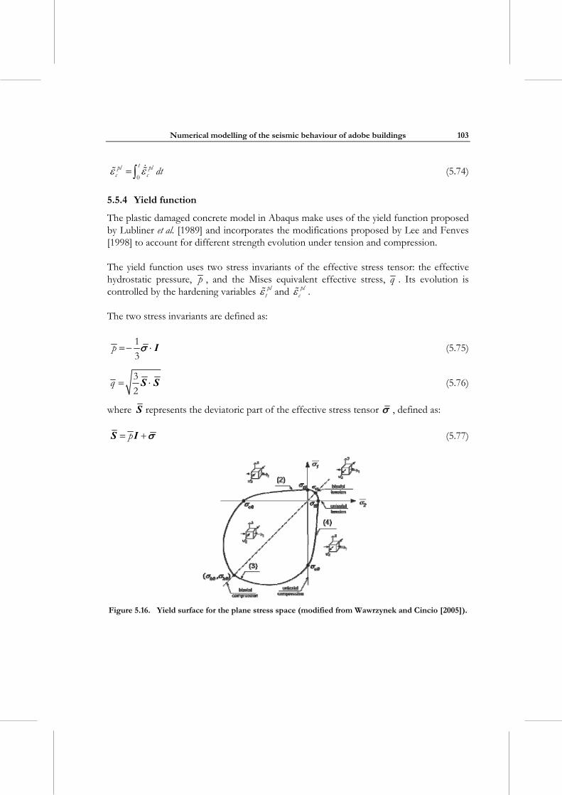
Numerical modelling of the seismic behaviour of adobe buildings
103
tpl plc c dt
0 (5.74)
5.5.4 Yield function
The plastic damaged concrete model in Abaqus make uses of the yield function proposed by Lubliner et al. [1989] and incorporates the modifications proposed by Lee and Fenves [1998] to account for different strength evolution under tension and compression.
The yield function uses two stress invariants of the effective stress tensor: the effective hydrostatic pressure, p , and the Mises equivalent effective stress, q . Its evolution is controlled by the hardening variables pl
t and plc .
The two stress invariants are defined as:
p1
3 I (5.75)
q3
2 S S (5.76)
where S represents the deviatoric part of the effective stress tensor , defined as:
p S I (5.77)
Figure 5.16. Yield surface for the plane stress space (modified from Wawrzynek and Cincio [2005]).
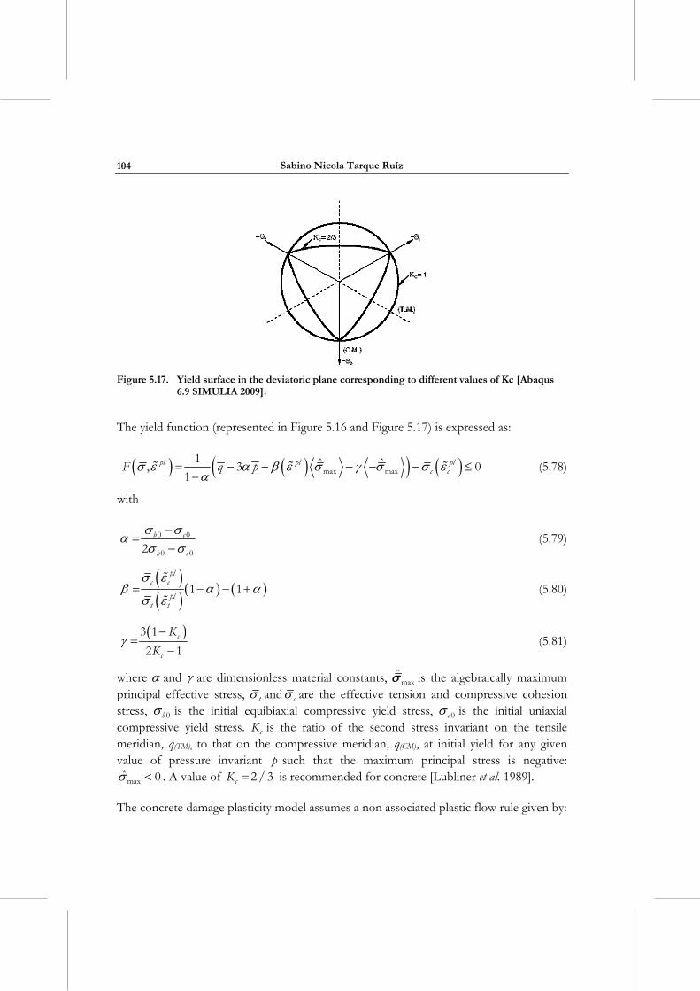
Sabino Nicola Tarque Ruíz
104
Figure 5.17. Yield surface in the deviatoric plane corresponding to different values of Kc [Abaqus
6.9 SIMULIA 2009].
The yield function (represented in Figure 5.16 and Figure 5.17) is expressed as:
pl pl plc cF q p max max
1 ˆ ˆ, 3 01
(5.78)
with
b c
b c
0 0
0 02
(5.79)
plc c
plt t
1 1
(5.80)
c
c
K
K
3 1
2 1
(5.81)
where and are dimensionless material constants, max is the algebraically maximum principal effective stress, t and c are the effective tension and compressive cohesion stress, b0 is the initial equibiaxial compressive yield stress, c 0 is the initial uniaxial compressive yield stress. cK is the ratio of the second stress invariant on the tensile meridian, q(TM), to that on the compressive meridian, q(CM), at initial yield for any given value of pressure invariant p such that the maximum principal stress is negative:
maxˆ 0 . A value of cK 2 / 3 is recommended for concrete [Lubliner et al. 1989].
The concrete damage plasticity model assumes a non associated plastic flow rule given by:
Numerical modelling of the seismic behaviour of adobe buildings
105
pl G
(5.82)
where is the nonnegative plastic multiplier. The flow potential G represents the Drucker-Praguer hyperbolic function:
tG e q p2 2
0 tan tan (5.83)
where e is a parameter, referred to as the eccentricity, that defines the rate at which the function approaches the asymptote (the flow potential tends to a straight line as the eccentricity tends to zero); t 0 is the uniaxial tensile stress at failure; and is the dilatation angle measured in the p q plane at high confining pressures. A low value of dilatancy is recommended for quasi-brittle materials [Malm 2009].
The recommended value for the eccentricity is e 0.1 , which implies that the material has almost the same dilatation angle over a wide range of confining pressure stress values [Abaqus 6.9 SIMULIA 2009].
5.5.5 Damage and stiffness degradation under uniaxial condition
5.5.5.1 Uniaxial behaviour
The uniaxial tensile and compressive response of concrete/masonry is characterized by damage plasticity. The stress-strain curves are also converted into stress versus plastic strain curves of the form:
pl plt t t t if, , , (5.84)
pl plc c c c if, , , (5.85)
where plt and pl
c are the equivalent plastic strains, plt and pl
c are the equivalent plastic strain rates, is the temperature, and if are other predefined field variables.
Figure 5.15a shows the tensile behaviour of the material, the elastic part is linear up to the failure stress t 0 . The failure corresponds to the onset of micro-cracking in the material. After this point, the formation of micro-cracks is represented macroscopically by softening stress-strain response. Under compression behaviour (Figure 5.15b), the material behaves linearly until the initial yield stress, c 0 . Thereafter, the material is characterized by stress hardening and stress softening after reaching the ultimate stress,
cu . When the specimen is unloaded from any part of the softening branch of the stress-
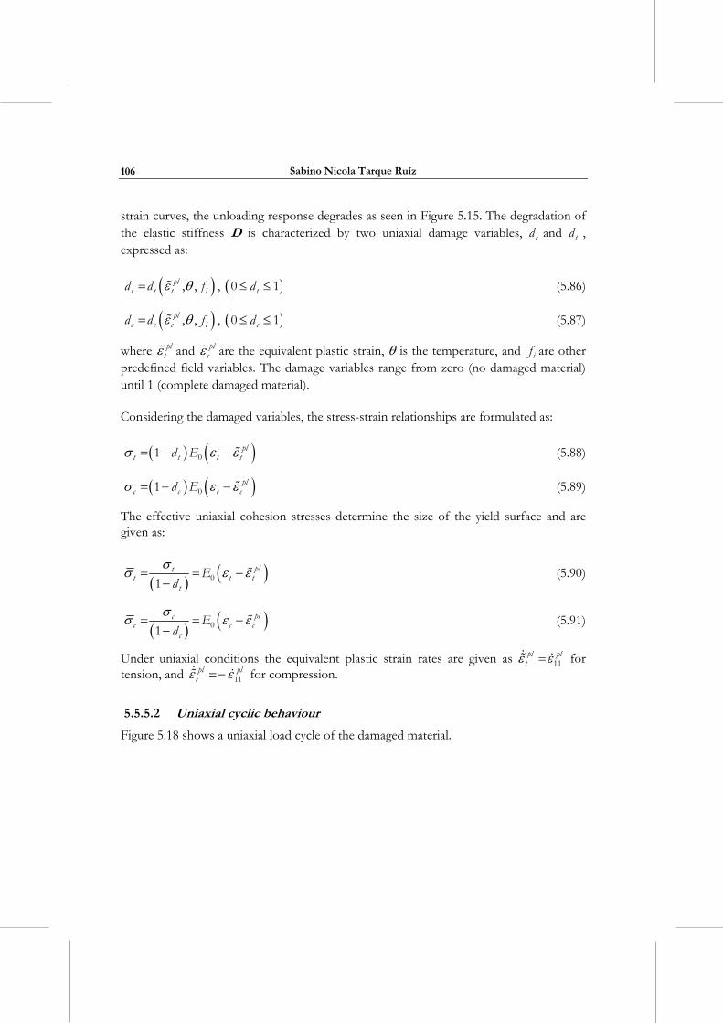
Sabino Nicola Tarque Ruíz
106
strain curves, the unloading response degrades as seen in Figure 5.15. The degradation of the elastic stiffness D is characterized by two uniaxial damage variables, cd and td , expressed as:
plt t t id d f, , , td0 1 (5.86)
plc c c id d f, , , cd0 1 (5.87)
where plt and pl
c are the equivalent plastic strain, is the temperature, and if are other predefined field variables. The damage variables range from zero (no damaged material) until 1 (complete damaged material).
Considering the damaged variables, the stress-strain relationships are formulated as:
plt t t td E01 (5.88)
plc c c cd E01 (5.89)
The effective uniaxial cohesion stresses determine the size of the yield surface and are given as:
pltt t t
t
Ed 01
(5.90)
plcc c c
c
Ed 01
(5.91)
Under uniaxial conditions the equivalent plastic strain rates are given as pl plt 11 for
tension, and pl plc 11 for compression.
5.5.5.2 Uniaxial cyclic behaviour
Figure 5.18 shows a uniaxial load cycle of the damaged material.
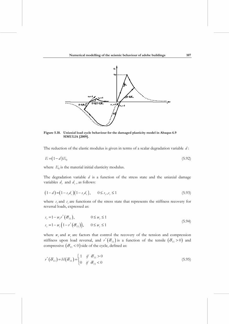
Numerical modelling of the seismic behaviour of adobe buildings
107
Figure 5.18. Uniaxial load cycle behaviour for the damaged plasticity model in Abaqus 6.9
SIMULIA [2009].
The reduction of the elastic modulus is given in terms of a scalar degradation variable d :
E d E01 (5.92)
where E0 is the material initial elasticity modulus.
The degradation variable d is a function of the stress state and the uniaxial damage variables td and cd , as follows:
t c c t t cd s d s d s s1 1 1 , 0 , 1 (5.93)
where ts and cs are functions of the stress state that represents the stiffness recovery for reversal loads, expressed as:
t t t
c c c
s w r w
s w r w
*11
*11
1 , 0 1
1 1 , 0 1
(5.94)
where tw and cw are factors that control the recovery of the tension and compression stiffness upon load reversal, and r *
11 is a function of the tensile 11 0 and compressive 11 0 side of the cycle, defined as:
if
r Hif
11*11 11
11
1 0
0 0
(5.95)
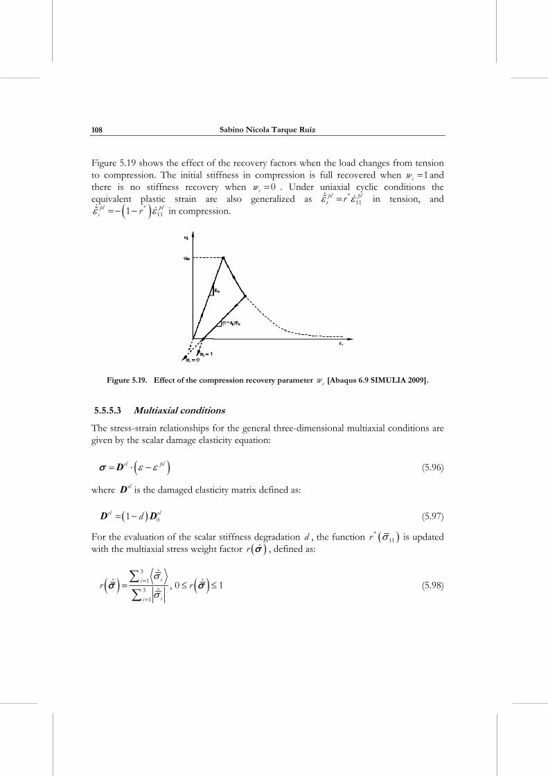
Sabino Nicola Tarque Ruíz
108
Figure 5.19 shows the effect of the recovery factors when the load changes from tension to compression. The initial stiffness in compression is full recovered when cw 1 and there is no stiffness recovery when cw 0 . Under uniaxial cyclic conditions the equivalent plastic strain are also generalized as pl pl
t r *11 in tension, and
pl plc r *
111 in compression.
Figure 5.19. Effect of the compression recovery parameter cw [Abaqus 6.9 SIMULIA 2009].
5.5.5.3 Multiaxial conditions
The stress-strain relationships for the general three-dimensional multiaxial conditions are given by the scalar damage elasticity equation:
el pl D (5.96)
where elD is the damaged elasticity matrix defined as:
el eld 01 D D (5.97)
For the evaluation of the scalar stiffness degradation d , the function r *11 is updated
with the multiaxial stress weight factor r , defined as:
ii
ii
r r
3
1
3
1
ˆˆ ˆ, 0 1
ˆ
(5.98)
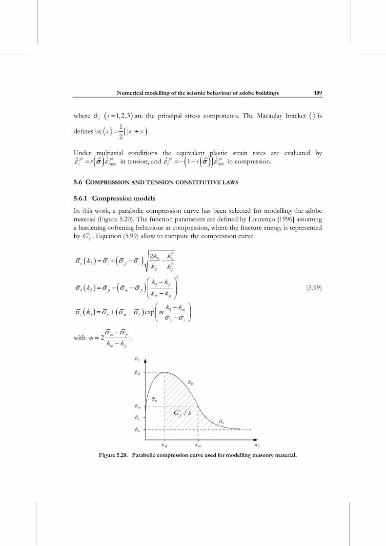
Numerical modelling of the seismic behaviour of adobe buildings
109
where i i 1, 2,3 are the principal stress components. The Macaulay bracket is
defines by x x x1
2 .
Under multiaxial conditions the equivalent plastic strain rates are evaluated by pl pl
t r maxˆˆ in tension, and pl pl
c r minˆˆ1 in compression.
5.6 COMPRESSION AND TENSION CONSTITUTIVE LAWS
5.6.1 Compression models
In this work, a parabolic compression curve has been selected for modelling the adobe material (Figure 5.20). The function parameters are defined by Lourenço [1996] assuming a hardening-softening behaviour in compression, where the fracture energy is represented by c
fG . Equation (5.99) allow to compute the compression curve.
a i p cp p
pb p m p
m p
mc r m r
r
k kk
k k
k kk
k k
k kk m
23 3
3 2
2
33
33
3
2
exp
(5.99)
with m p
m p
mk k
2
.
Figure 5.20. Parabolic compression curve used for modelling masonry material.
cfG h/
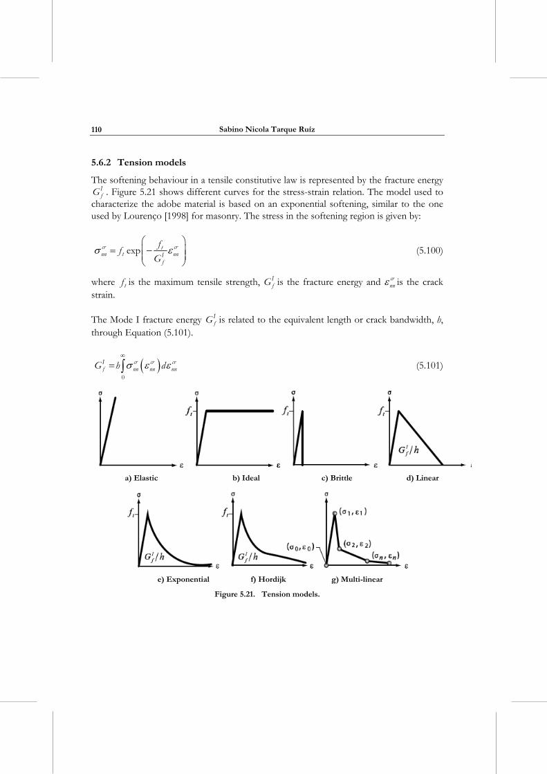
Sabino Nicola Tarque Ruíz
110
5.6.2 Tension models
The softening behaviour in a tensile constitutive law is represented by the fracture energy IfG . Figure 5.21 shows different curves for the stress-strain relation. The model used to
characterize the adobe material is based on an exponential softening, similar to the one used by Lourenço [1998] for masonry. The stress in the softening region is given by:
cr crtnn t nnI
f
ff
Gexp
(5.100)
where tf is the maximum tensile strength, IfG is the fracture energy and cr
nn is the crack strain.
The Mode I fracture energy IfG is related to the equivalent length or crack bandwidth, h,
through Equation (5.101).
I cr cr crf nn nn nnG h d
0
(5.101)
a) Elastic b) Ideal c) Brittle d) Linear
e) Exponential f) Hordijk g) Multi-linear
Figure 5.21. Tension models.
Numerical modelling of the seismic behaviour of adobe buildings
111
5.7 SUMMARY
The numerical modelling of cracking and damage in concrete/masonry panels is based on discrete mechanics and continuum mechanics, and that plasticity based models are suitable for micro and macro modelling of masonry. In this chapter, a review of the theory of plasticity as well as a description of the formulation for discrete (i.e. fracture mechanics) and continuum models are given.
For the discrete model the combined cracking-shearing-crushing model is given here. For the continuum model two approaches are described: the smear crack approach and a damage plasticity based model. These models are going to be used in the following chapters with two finite element programmes: Midas FEA and Abaqus. Unlike smeared crack models, the damaged plasticity model represents the cracking behaviour by damage factors that modify the constitutive laws for unloading.
Two formulations of the smeared crack models are discussed: decomposed-strain model and total-strain model. The first one separates the elastic and crack strain for computing stress levels, while the second one makes used of the total material strain for computing stress levels at the integration points.
Finally, constitutive laws for representation of tension and compression behaviour are reported. In this work, the compression of adobe masonry in the inelastic range is represented by a parabolic function and the tension by an exponential function. The inelastic material parameters for adobe masonry are shown in the next chapter.

6. NON-LINEAR PSEUDO-STATIC ANALYSIS OF ADOBE WALLS
Blondet et al. [2005] carried out a cyclic test on an adobe wall to reproduce its seismic response and damage pattern under in-plane loads. The displacement was applied at the wall top and at low increments to simulate a static analysis. In this work, the force-displacement curve obtained from the experimental test (see section 3.5) is used for calibrating preliminary numerical models of adobe walls.
In the previous chapter different modelling approaches were described for representing the cracking and damage on concrete panels, which are also applied to masonry panels, including adobe walls. These numerical approaches are divided into discrete and continuum models.
The numerical modelling of adobe structures is not simple since there is scarce material information, especially the fracture energy in tension and compression for modelling the inelastic behaviour of the adobe material. In this chapter three finite element models of adobe walls are built and, taking advantage of the experimental results shown in 3.5.3, the adobe material properties are calibrated within a discrete and continuum approach. For this, two finite element programmes are used: Midas FEA and Abaqus/Standard. In Midas FEA two finite element models are built, one following the simplified micro-modelling (discrete model) and the second one following a smeared crack model (continuum model). The adobe wall built in Abaqus/Standard is modelled following a damaged plasticity model (continuum model). The finite element models are solved following an implicit solution, and are described as follows.
6.1 IMPLICIT SOLUTION METHOD FOR SOLVING QUASI-STATIC PROBLEMS
In this analysis the load/displacement is applied slowly to the body so that the inertial forces can be neglected (acceleration and velocities are zero). It follows that the internal forces I (for a given displacement u ) must be equal to the external forces P at each time step t , or the residual force R u must be:
R u = P I u 0 (6.1)
Sabino Nicola Tarque Ruíz
114
Amongst the different solution procedures used in the implicit finite element solvers, the Newton-Raphson solution procedure is the faster for solving non-linear problems under force control, though no convergence procedure is full proof. When solving quasi static problems, a set of non-linear equations are generally expressed as:
T T
V SdV dS 0G u B u N t (6.2)
where G is a set of non-linear equations in u which are updated at each iteration and are function of the nodal displacements vector u , is the stresses vector, B is the matrix that relates the strain vector to the displacements, N is the matrix of element shape functions and t is the surface traction vector. V and S represent the volume and surface of the body, respectively. The right-hand side of Equation (6.2) represents the difference between the internal and the external forces.
Equation (6.2) is solved for a displacement vector that equilibrates the internal and external forces, as explained in Harewood and McHugh [2007]. Besides, Equation (6.2) is solved by incremental methods where load/displacements are applied in time steps t ,
t tu is solved from a known state tu . In the following equations the subscript denotes iteration number and the superscript denotes an increment step.
At the beginning, Equation (6.2) is solved to obtain the displacement correction t ti 1
u
based on information of t ti
u as:
t tit t t t
i i
1
1
G uu G u
u (6.3)
The partial derivative on the right side is the so called Jacobian matrix expressed as the global stiffness matrix tanK :
t tit t
itan
G uK u =
u (6.4)
Thus:
t t t t t ti i i
1
1 tan
u K u G u (6.5)
The previous equation involves the inversion of the global stiffness matrix (no singular matrix), which ends in a computationally expensive operation, but it ensures that a
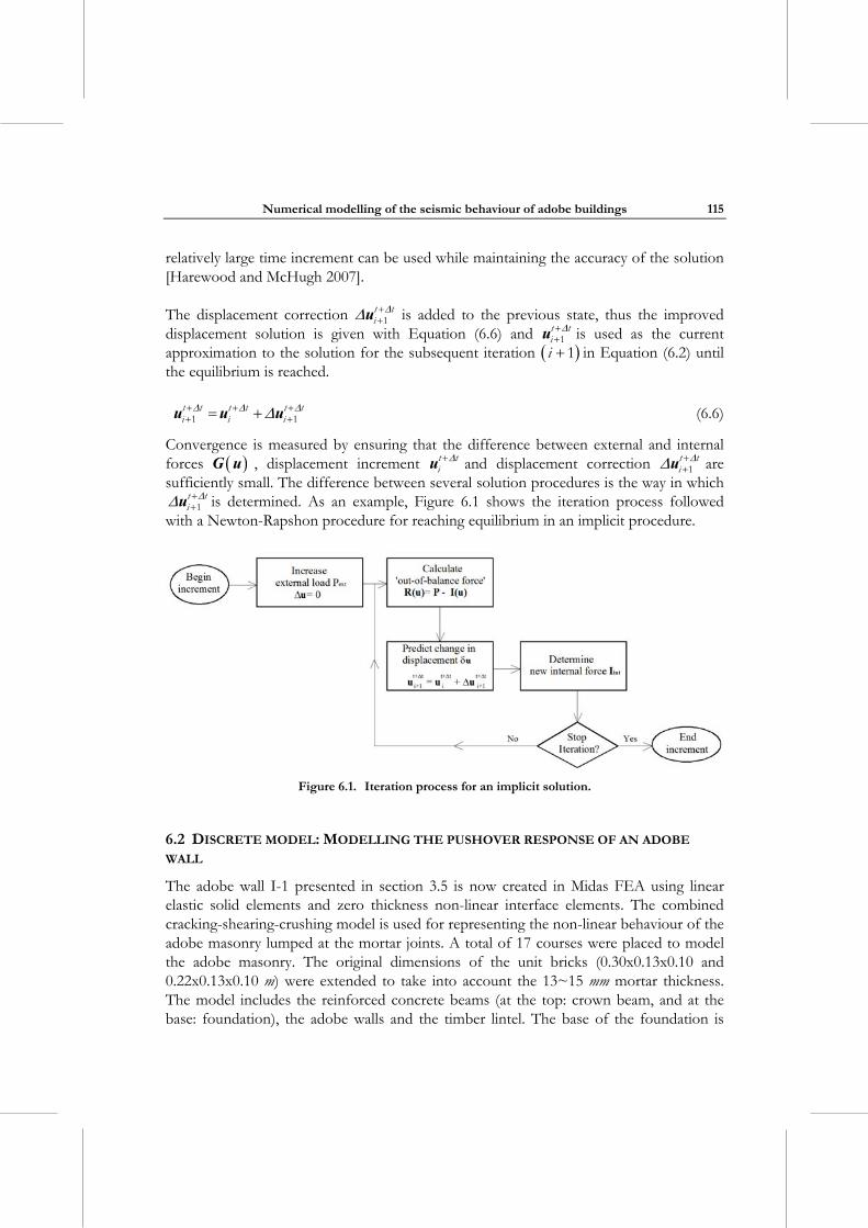
Numerical modelling of the seismic behaviour of adobe buildings
115
relatively large time increment can be used while maintaining the accuracy of the solution [Harewood and McHugh 2007].
The displacement correction t ti 1
u is added to the previous state, thus the improved
displacement solution is given with Equation (6.6) and t ti 1
u is used as the current
approximation to the solution for the subsequent iteration i 1 in Equation (6.2) until the equilibrium is reached.
t t t t t ti i i1 1
u u u (6.6)
Convergence is measured by ensuring that the difference between external and internal forces G u , displacement increment t t
iu and displacement correction t t
i 1
u are sufficiently small. The difference between several solution procedures is the way in which
t ti 1
u is determined. As an example, Figure 6.1 shows the iteration process followed
with a Newton-Rapshon procedure for reaching equilibrium in an implicit procedure.
Figure 6.1. Iteration process for an implicit solution.
6.2 DISCRETE MODEL: MODELLING THE PUSHOVER RESPONSE OF AN ADOBE
WALL
The adobe wall I-1 presented in section 3.5 is now created in Midas FEA using linear elastic solid elements and zero thickness non-linear interface elements. The combined cracking-shearing-crushing model is used for representing the non-linear behaviour of the adobe masonry lumped at the mortar joints. A total of 17 courses were placed to model the adobe masonry. The original dimensions of the unit bricks (0.30x0.13x0.10 and 0.22x0.13x0.10 m) were extended to take into account the 13~15 mm mortar thickness. The model includes the reinforced concrete beams (at the top: crown beam, and at the base: foundation), the adobe walls and the timber lintel. The base of the foundation is
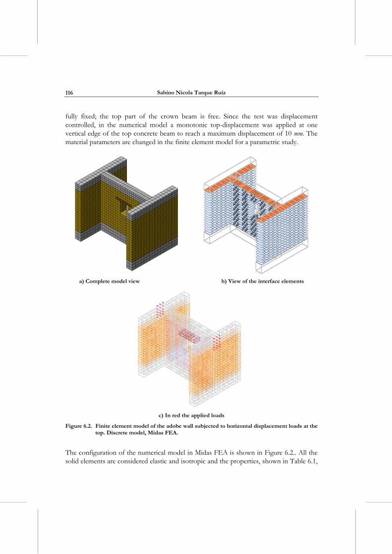
Sabino Nicola Tarque Ruíz
116
fully fixed; the top part of the crown beam is free. Since the test was displacement controlled, in the numerical model a monotonic top-displacement was applied at one vertical edge of the top concrete beam to reach a maximum displacement of 10 mm. The material parameters are changed in the finite element model for a parametric study.
a) Complete model view b) View of the interface elements
c) In red the applied loads
Figure 6.2. Finite element model of the adobe wall subjected to horizontal displacement loads at the top. Discrete model, Midas FEA.
The configuration of the numerical model in Midas FEA is shown in Figure 6.2.. All the solid elements are considered elastic and isotropic and the properties, shown in Table 6.1,
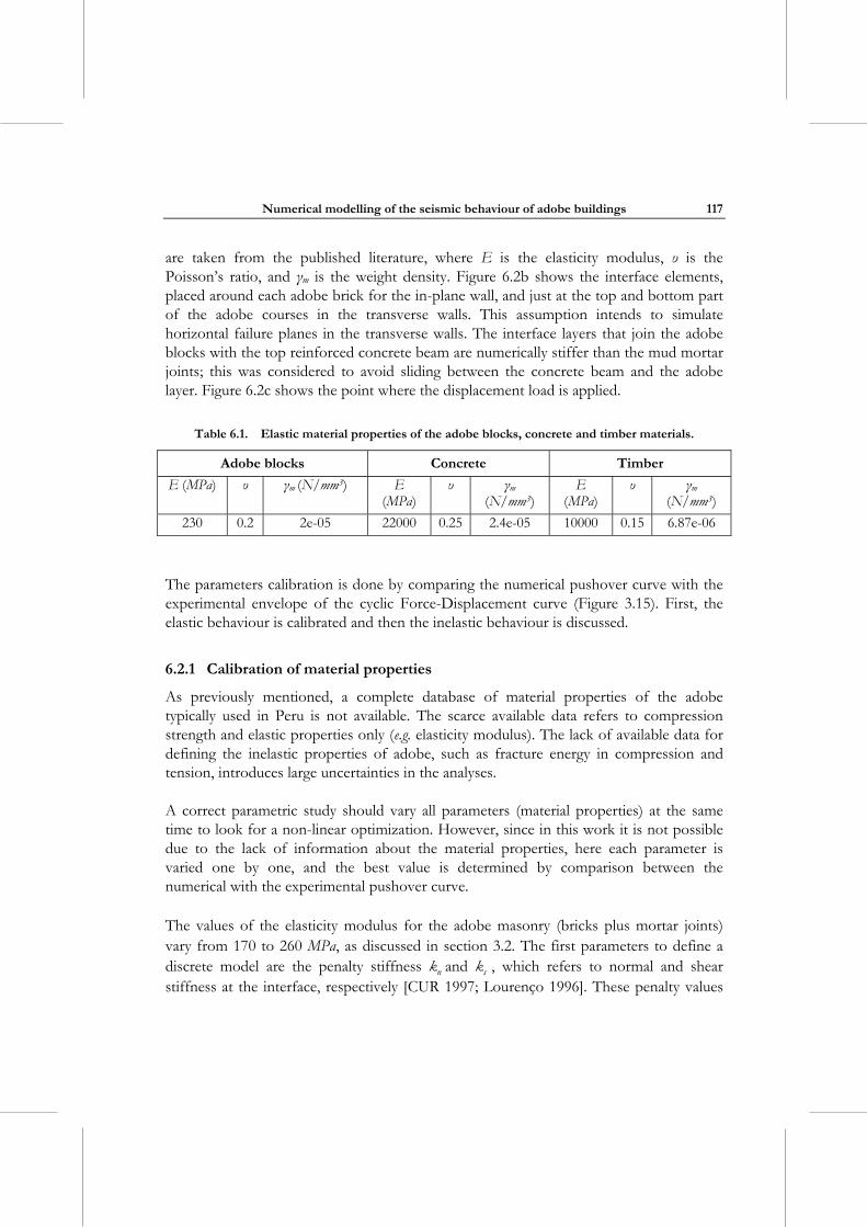
Numerical modelling of the seismic behaviour of adobe buildings
117
are taken from the published literature, where E is the elasticity modulus, υ is the Poisson’s ratio, and γm is the weight density. Figure 6.2b shows the interface elements, placed around each adobe brick for the in-plane wall, and just at the top and bottom part of the adobe courses in the transverse walls. This assumption intends to simulate horizontal failure planes in the transverse walls. The interface layers that join the adobe blocks with the top reinforced concrete beam are numerically stiffer than the mud mortar joints; this was considered to avoid sliding between the concrete beam and the adobe layer. Figure 6.2c shows the point where the displacement load is applied.
Table 6.1. Elastic material properties of the adobe blocks, concrete and timber materials.
Adobe blocks Concrete Timber
E (MPa) υ γm (N/mm3) E (MPa)
υ γm
(N/mm3) E
(MPa) υ γm
(N/mm3)
230 0.2 2e-05 22000 0.25 2.4e-05 10000 0.15 6.87e-06
The parameters calibration is done by comparing the numerical pushover curve with the experimental envelope of the cyclic Force-Displacement curve (Figure 3.15). First, the elastic behaviour is calibrated and then the inelastic behaviour is discussed.
6.2.1 Calibration of material properties
As previously mentioned, a complete database of material properties of the adobe typically used in Peru is not available. The scarce available data refers to compression strength and elastic properties only (e.g. elasticity modulus). The lack of available data for defining the inelastic properties of adobe, such as fracture energy in compression and tension, introduces large uncertainties in the analyses.
A correct parametric study should vary all parameters (material properties) at the same time to look for a non-linear optimization. However, since in this work it is not possible due to the lack of information about the material properties, here each parameter is varied one by one, and the best value is determined by comparison between the numerical with the experimental pushover curve.
The values of the elasticity modulus for the adobe masonry (bricks plus mortar joints) vary from 170 to 260 MPa, as discussed in section 3.2. The first parameters to define a discrete model are the penalty stiffness nk and sk , which refers to normal and shear stiffness at the interface, respectively [CUR 1997; Lourenço 1996]. These penalty values
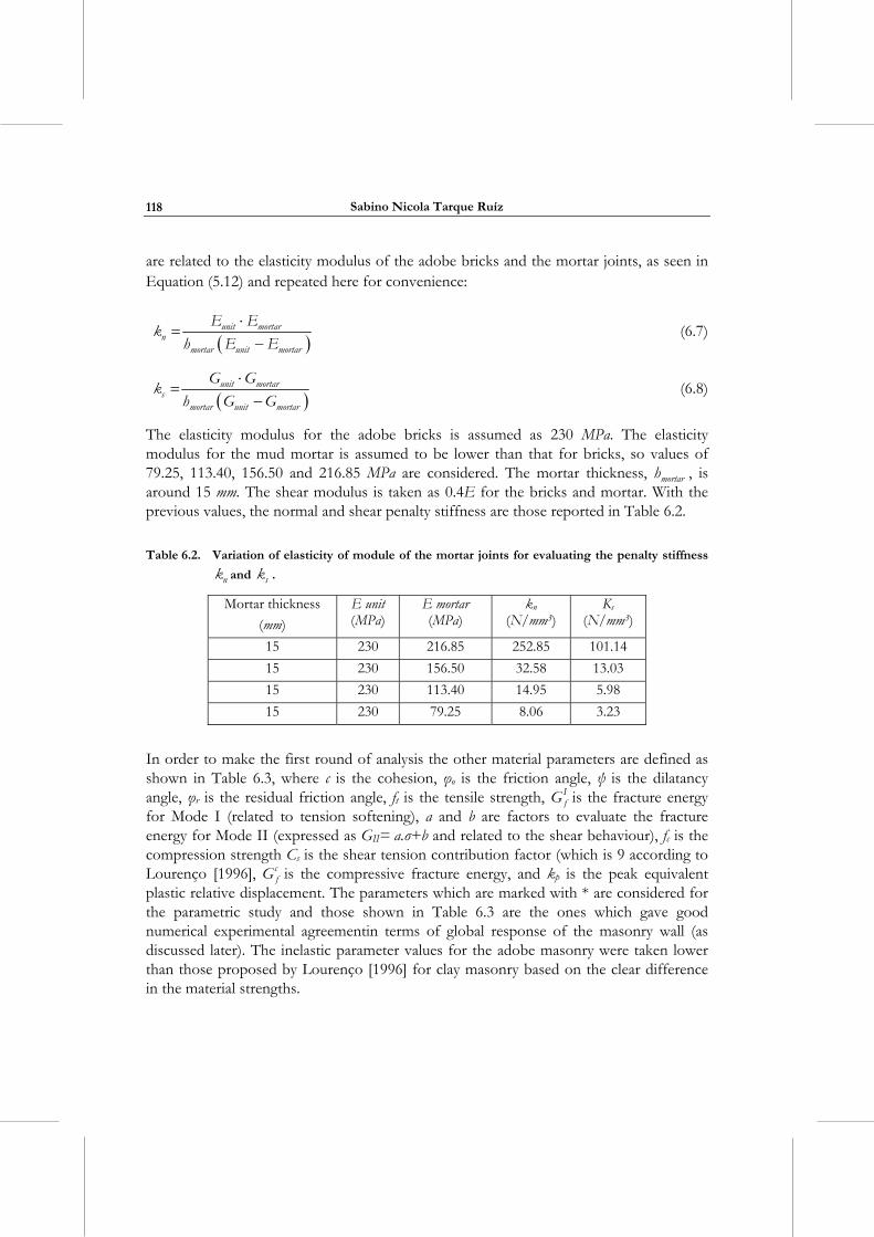
Sabino Nicola Tarque Ruíz
118
are related to the elasticity modulus of the adobe bricks and the mortar joints, as seen in Equation (5.12) and repeated here for convenience:
unit mortar
nmortar unit mortar
E Ek
h E E
(6.7)
unit mortar
smortar unit mortar
G Gk
h G G
(6.8)
The elasticity modulus for the adobe bricks is assumed as 230 MPa. The elasticity modulus for the mud mortar is assumed to be lower than that for bricks, so values of 79.25, 113.40, 156.50 and 216.85 MPa are considered. The mortar thickness, mortarh , is around 15 mm. The shear modulus is taken as 0.4E for the bricks and mortar. With the previous values, the normal and shear penalty stiffness are those reported in Table 6.2.
Table 6.2. Variation of elasticity of module of the mortar joints for evaluating the penalty stiffness
nk and sk .
Mortar thickness
(mm)
E unit (MPa)
E mortar (MPa)
kn
(N/mm3) Ks
(N/mm3)
15 230 216.85 252.85 101.14
15 230 156.50 32.58 13.03
15 230 113.40 14.95 5.98
15 230 79.25 8.06 3.23
In order to make the first round of analysis the other material parameters are defined as shown in Table 6.3, where c is the cohesion, φo is the friction angle, ψ is the dilatancy angle, φr is the residual friction angle, ft is the tensile strength, I
fG is the fracture energy for Mode I (related to tension softening), a and b are factors to evaluate the fracture energy for Mode II (expressed as GII= a.σ+b and related to the shear behaviour), fc is the compression strength Cs is the shear tension contribution factor (which is 9 according to Lourenço [1996], c
fG is the compressive fracture energy, and kp is the peak equivalent plastic relative displacement. The parameters which are marked with * are considered for the parametric study and those shown in Table 6.3 are the ones which gave good numerical experimental agreementin terms of global response of the masonry wall (as discussed later). The inelastic parameter values for the adobe masonry were taken lower than those proposed by Lourenço [1996] for clay masonry based on the clear difference in the material strengths.
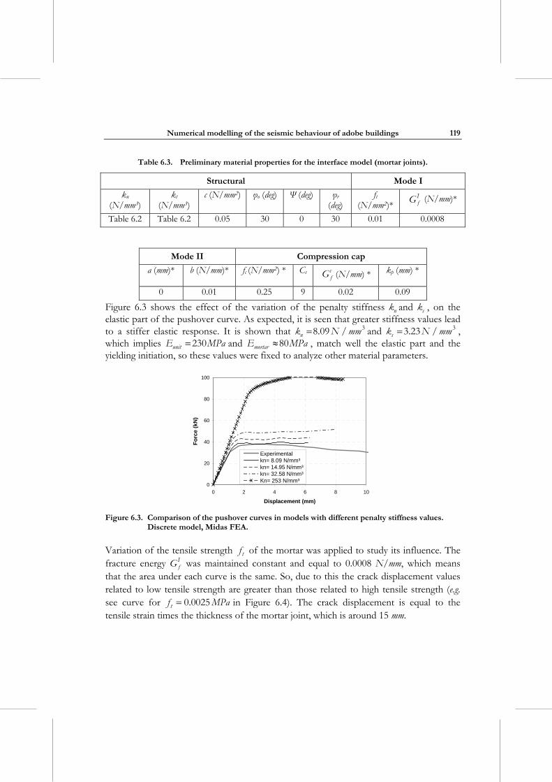
Numerical modelling of the seismic behaviour of adobe buildings
119
Table 6.3. Preliminary material properties for the interface model (mortar joints).
Structural Mode I
kn
(N/mm3) kt
(N/mm3) c (N/mm2) φo (deg) Ψ (deg) φr
(deg) ft
(N/mm2)* IfG (N/mm)*
Table 6.2 Table 6.2 0.05 30 0 30 0.01 0.0008
Mode II Compression cap
a (mm)* b (N/mm)* fc (N/mm2) * Cs cfG (N/mm) * kp (mm) *
0 0.01 0.25 9 0.02 0.09
Figure 6.3 shows the effect of the variation of the penalty stiffness nk and sk , on the elastic part of the pushover curve. As expected, it is seen that greater stiffness values lead to a stiffer elastic response. It is shown that nk N mm38.09 / and sk N mm33.23 / , which implies unitE MPa230 and mortarE MPa80 , match well the elastic part and the yielding initiation, so these values were fixed to analyze other material parameters.
0
20
40
60
80
100
0 2 4 6 8 10
Displacement (mm)
Fo
rce
(kN
)
Experimentalkn= 8.09 N/mm³kn= 14.95 N/mm³kn= 32.58 N/mm³Kn= 253 N/mm³
Figure 6.3. Comparison of the pushover curves in models with different penalty stiffness values.
Discrete model, Midas FEA.
Variation of the tensile strength tf of the mortar was applied to study its influence. The fracture energy I
fG was maintained constant and equal to 0.0008 N/mm, which means that the area under each curve is the same. So, due to this the crack displacement values related to low tensile strength are greater than those related to high tensile strength (e.g. see curve for tf MPa0.0025 in Figure 6.4). The crack displacement is equal to the tensile strain times the thickness of the mortar joint, which is around 15 mm.
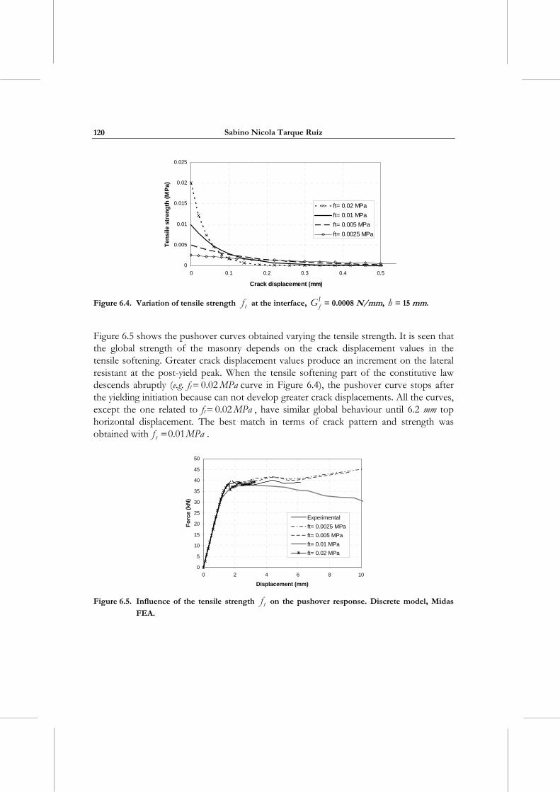
Sabino Nicola Tarque Ruíz
120
0
0.005
0.01
0.015
0.02
0.025
0 0.1 0.2 0.3 0.4 0.5
Crack displacement (mm)
Ten
sile
str
eng
th (
MP
a)
ft= 0.02 MPa
ft= 0.01 MPa
ft= 0.005 MPa
ft= 0.0025 MPa
Figure 6.4. Variation of tensile strength tf at the interface, IfG = 0.0008 N/mm, h = 15 mm.
Figure 6.5 shows the pushover curves obtained varying the tensile strength. It is seen that the global strength of the masonry depends on the crack displacement values in the tensile softening. Greater crack displacement values produce an increment on the lateral resistant at the post-yield peak. When the tensile softening part of the constitutive law descends abruptly (e.g. ft MPa0.02 curve in Figure 6.4), the pushover curve stops after the yielding initiation because can not develop greater crack displacements. All the curves, except the one related to ft MPa0.02 , have similar global behaviour until 6.2 mm top horizontal displacement. The best match in terms of crack pattern and strength was obtained with tf MPa0.01 .
0
5
10
15
20
25
30
35
40
45
50
0 2 4 6 8 10
Displacement (mm)
Fo
rce
(kN
)
Experimental
ft= 0.0025 MPa
ft= 0.005 MPa
ft= 0.01 MPa
ft= 0.02 MPa
Figure 6.5. Influence of the tensile strength tf on the pushover response. Discrete model, Midas
FEA.
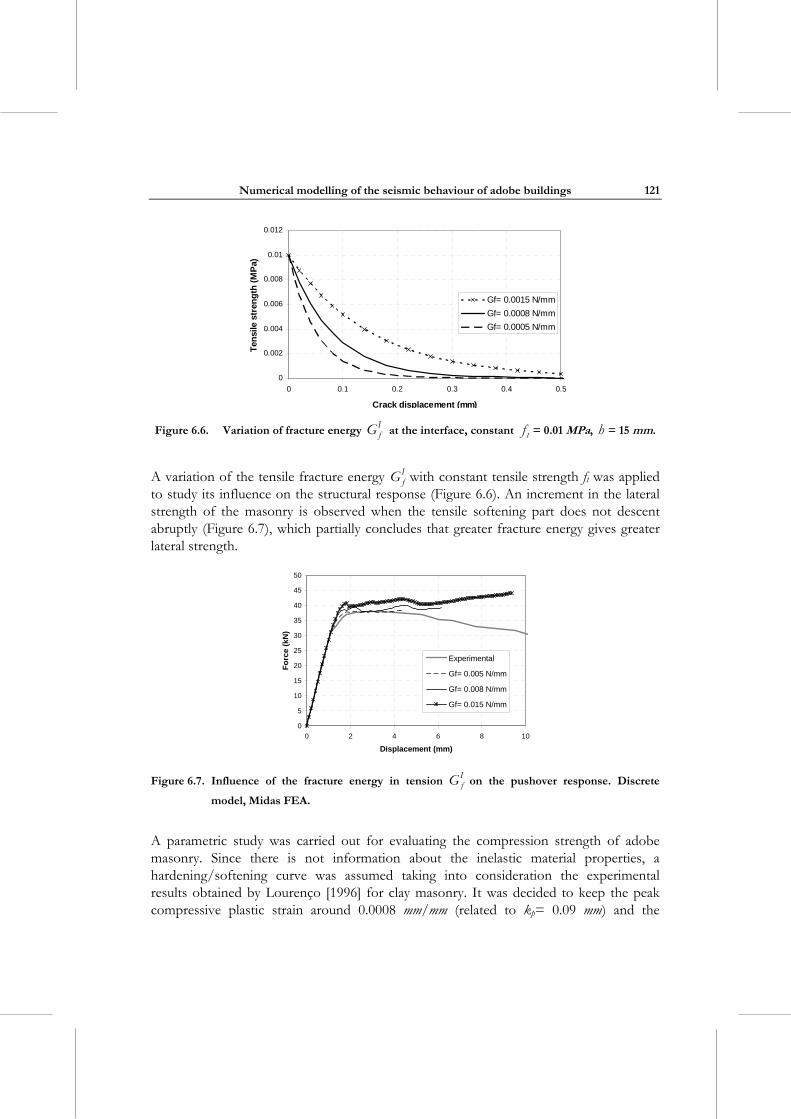
Numerical modelling of the seismic behaviour of adobe buildings
121
0
0.002
0.004
0.006
0.008
0.01
0.012
0 0.1 0.2 0.3 0.4 0.5
Crack displacement (mm)
Ten
sile
str
eng
th (
MP
a)
Gf= 0.0015 N/mm
Gf= 0.0008 N/mm
Gf= 0.0005 N/mm
Figure 6.6. Variation of fracture energy IfG at the interface, constant tf = 0.01 MPa, h = 15 mm.
A variation of the tensile fracture energy IfG with constant tensile strength ft was applied
to study its influence on the structural response (Figure 6.6). An increment in the lateral strength of the masonry is observed when the tensile softening part does not descent abruptly (Figure 6.7), which partially concludes that greater fracture energy gives greater lateral strength.
0
5
10
15
20
25
30
35
40
45
50
0 2 4 6 8 10
Displacement (mm)
Fo
rce
(kN
)
Experimental
Gf= 0.005 N/mm
Gf= 0.008 N/mm
Gf= 0.015 N/mm
Figure 6.7. Influence of the fracture energy in tension IfG on the pushover response. Discrete
model, Midas FEA.
A parametric study was carried out for evaluating the compression strength of adobe masonry. Since there is not information about the inelastic material properties, a hardening/softening curve was assumed taking into consideration the experimental results obtained by Lourenço [1996] for clay masonry. It was decided to keep the peak compressive plastic strain around 0.0008 mm/mm (related to kp= 0.09 mm) and the
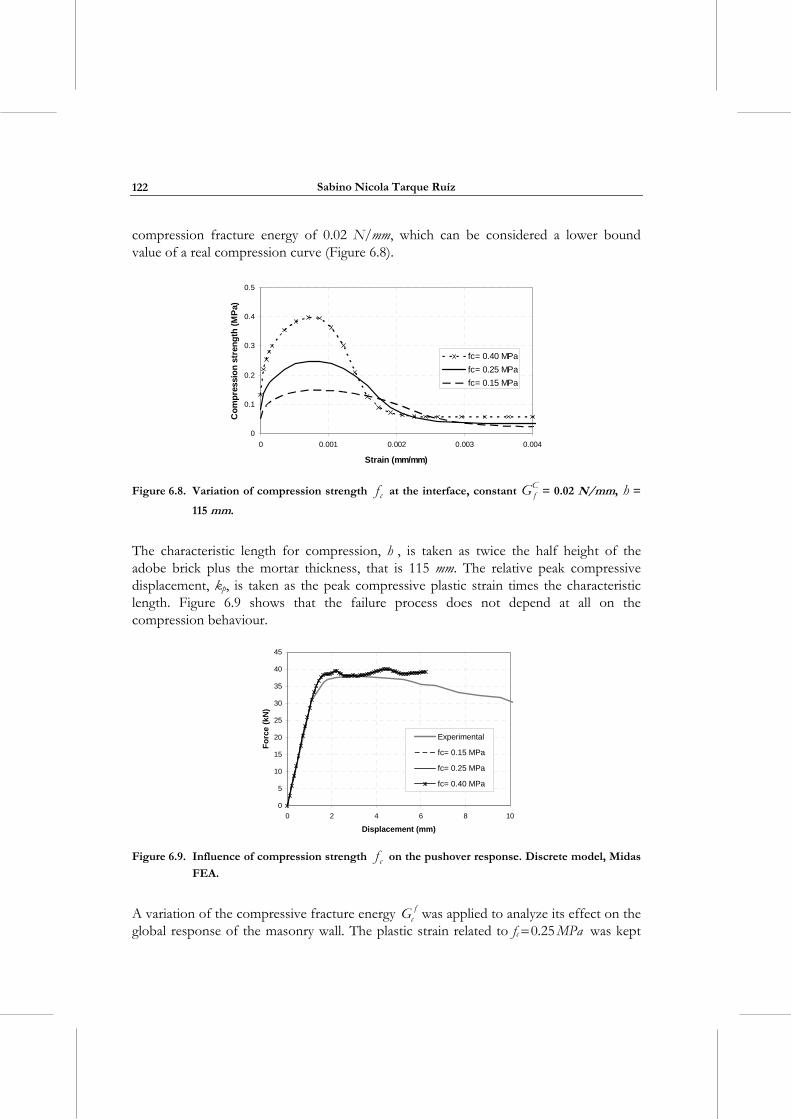
Sabino Nicola Tarque Ruíz
122
compression fracture energy of 0.02 N/mm, which can be considered a lower bound value of a real compression curve (Figure 6.8).
0
0.1
0.2
0.3
0.4
0.5
0 0.001 0.002 0.003 0.004
Strain (mm/mm)
Co
mp
ress
ion
str
eng
th (
MP
a)
fc= 0.40 MPa
fc= 0.25 MPa
fc= 0.15 MPa
Figure 6.8. Variation of compression strength cf at the interface, constant CfG = 0.02 N/mm, h =
115 mm.
The characteristic length for compression, h , is taken as twice the half height of the adobe brick plus the mortar thickness, that is 115 mm. The relative peak compressive displacement, kp, is taken as the peak compressive plastic strain times the characteristic length. Figure 6.9 shows that the failure process does not depend at all on the compression behaviour.
0
5
10
15
20
25
30
35
40
45
0 2 4 6 8 10
Displacement (mm)
Fo
rce
(k
N)
Experimental
fc= 0.15 MPa
fc= 0.25 MPa
fc= 0.40 MPa
Figure 6.9. Influence of compression strength cf on the pushover response. Discrete model, Midas
FEA.
A variation of the compressive fracture energy fcG was applied to analyze its effect on the
global response of the masonry wall. The plastic strain related to fc MPa0.25 was kept
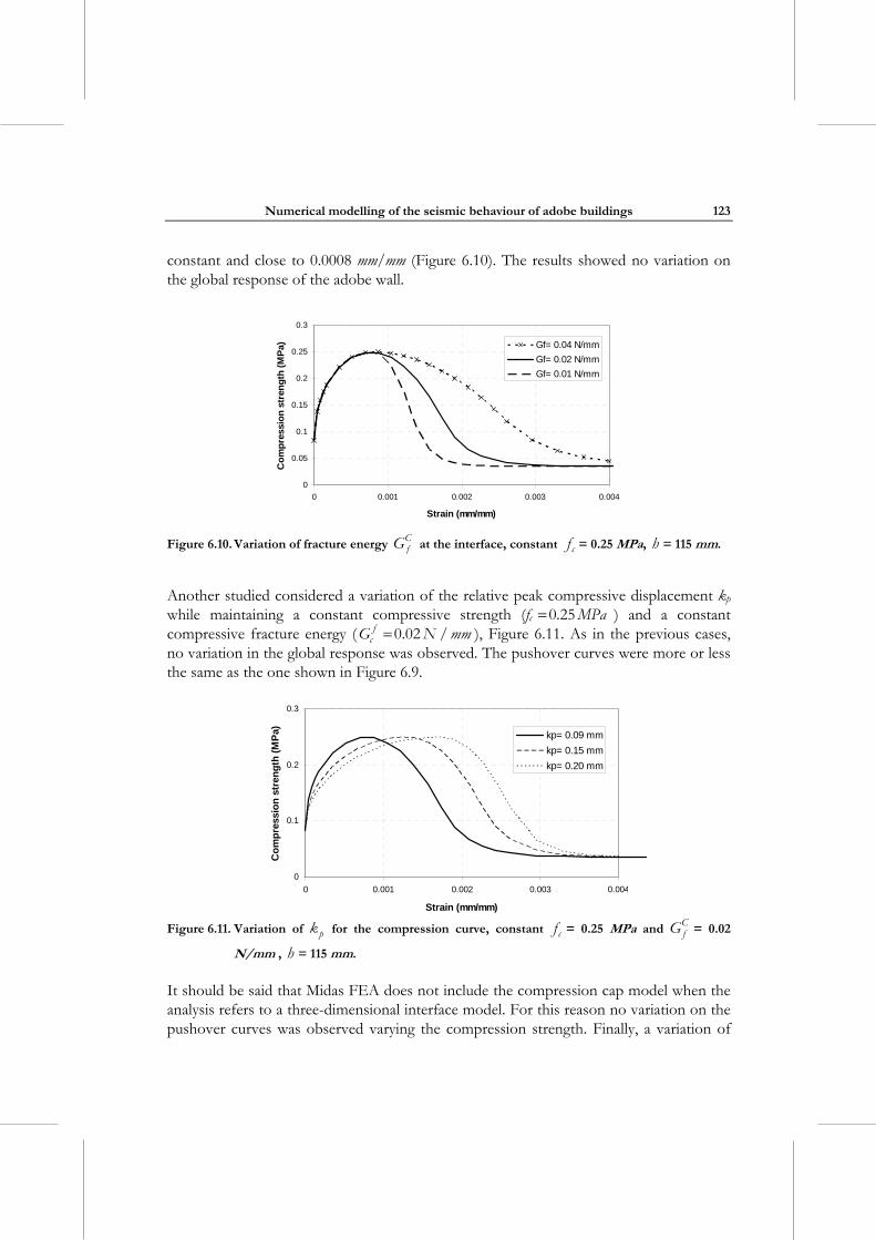
Numerical modelling of the seismic behaviour of adobe buildings
123
constant and close to 0.0008 mm/mm (Figure 6.10). The results showed no variation on the global response of the adobe wall.
0
0.05
0.1
0.15
0.2
0.25
0.3
0 0.001 0.002 0.003 0.004
Strain (mm/mm)
Co
mp
ress
ion
str
eng
th (
MP
a) Gf= 0.04 N/mm
Gf= 0.02 N/mm
Gf= 0.01 N/mm
Figure 6.10. Variation of fracture energy CfG at the interface, constant cf = 0.25 MPa, h = 115 mm.
Another studied considered a variation of the relative peak compressive displacement kp
while maintaining a constant compressive strength (fc MPa0.25 ) and a constant compressive fracture energy ( f
cG N mm0.02 / ), Figure 6.11. As in the previous cases, no variation in the global response was observed. The pushover curves were more or less the same as the one shown in Figure 6.9.
0
0.1
0.2
0.3
0 0.001 0.002 0.003 0.004
Strain (mm/mm)
Co
mp
ress
ion
str
eng
th (
MP
a) kp= 0.09 mm
kp= 0.15 mm
kp= 0.20 mm
Figure 6.11. Variation of pk for the compression curve, constant cf = 0.25 MPa and C
fG = 0.02
N/mm , h = 115 mm.
It should be said that Midas FEA does not include the compression cap model when the analysis refers to a three-dimensional interface model. For this reason no variation on the pushover curves was observed varying the compression strength. Finally, a variation of
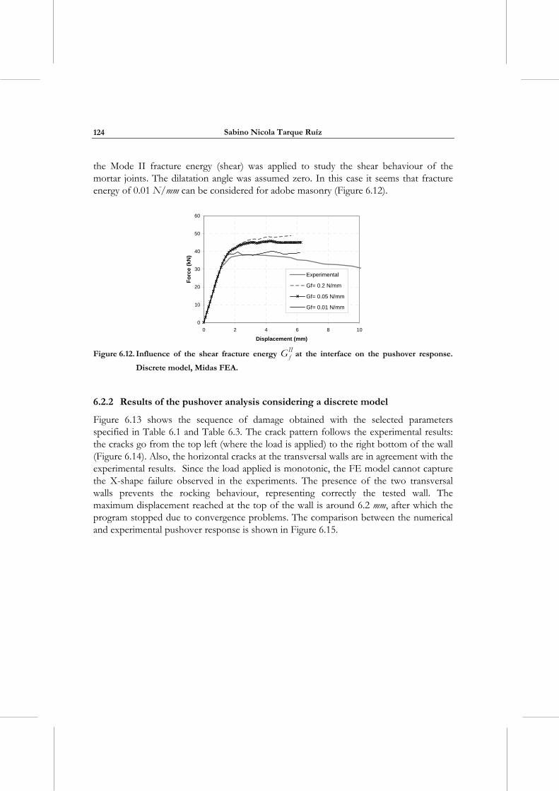
Sabino Nicola Tarque Ruíz
124
the Mode II fracture energy (shear) was applied to study the shear behaviour of the mortar joints. The dilatation angle was assumed zero. In this case it seems that fracture energy of 0.01 N/mm can be considered for adobe masonry (Figure 6.12).
0
10
20
30
40
50
60
0 2 4 6 8 10
Displacement (mm)
Fo
rce
(kN
)
Experimental
Gf= 0.2 N/mm
Gf= 0.05 N/mm
Gf= 0.01 N/mm
Figure 6.12. Influence of the shear fracture energy II
fG at the interface on the pushover response.
Discrete model, Midas FEA.
6.2.2 Results of the pushover analysis considering a discrete model
Figure 6.13 shows the sequence of damage obtained with the selected parameters specified in Table 6.1 and Table 6.3. The crack pattern follows the experimental results: the cracks go from the top left (where the load is applied) to the right bottom of the wall (Figure 6.14). Also, the horizontal cracks at the transversal walls are in agreement with the experimental results. Since the load applied is monotonic, the FE model cannot capture the X-shape failure observed in the experiments. The presence of the two transversal walls prevents the rocking behaviour, representing correctly the tested wall. The maximum displacement reached at the top of the wall is around 6.2 mm, after which the program stopped due to convergence problems. The comparison between the numerical and experimental pushover response is shown in Figure 6.15.
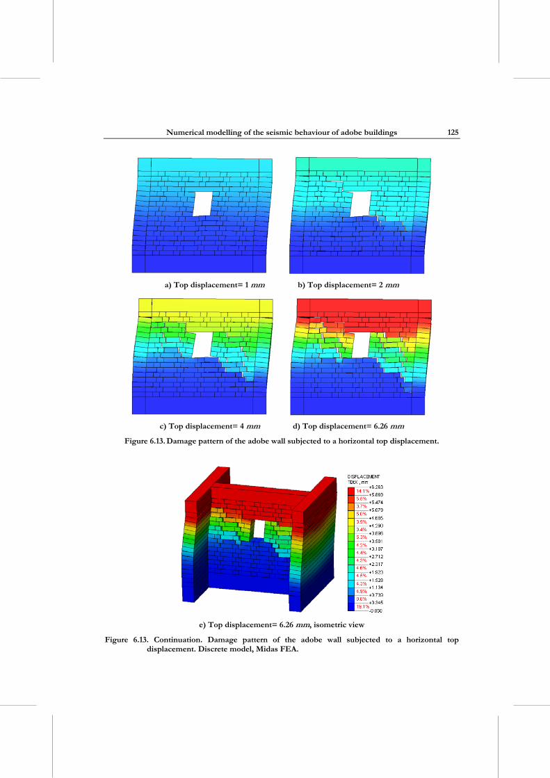
Numerical modelling of the seismic behaviour of adobe buildings
125
a) Top displacement= 1 mm b) Top displacement= 2 mm
c) Top displacement= 4 mm d) Top displacement= 6.26 mm
Figure 6.13. Damage pattern of the adobe wall subjected to a horizontal top displacement.
e) Top displacement= 6.26 mm, isometric view
Figure 6.13. Continuation. Damage pattern of the adobe wall subjected to a horizontal top displacement. Discrete model, Midas FEA.
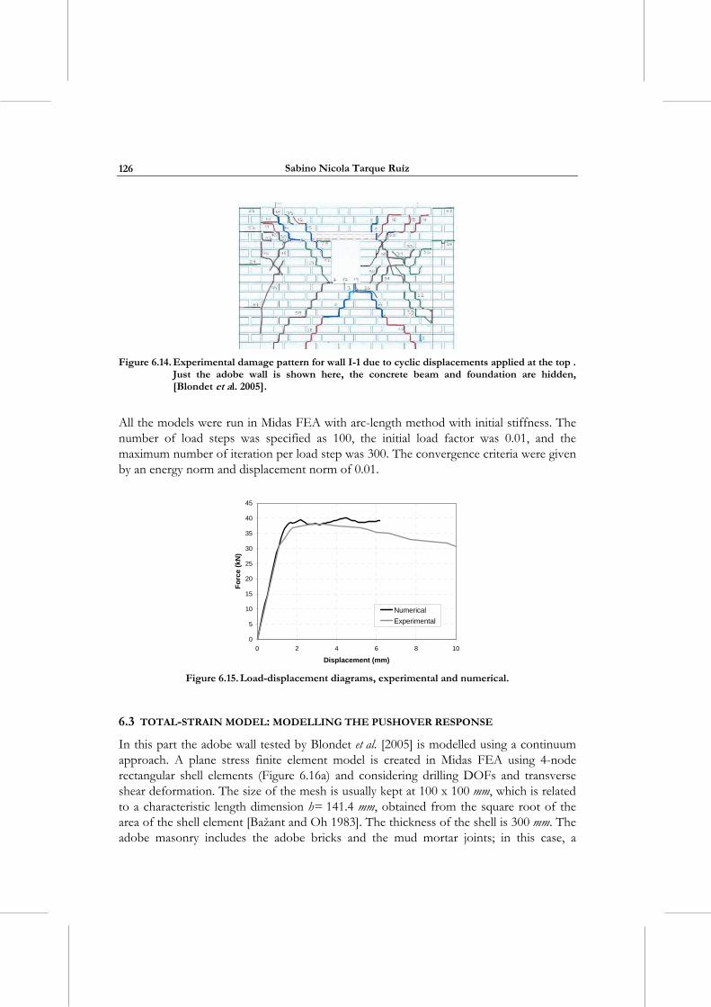
Sabino Nicola Tarque Ruíz
126
Figure 6.14. Experimental damage pattern for wall I-1 due to cyclic displacements applied at the top .
Just the adobe wall is shown here, the concrete beam and foundation are hidden, [Blondet et al. 2005].
All the models were run in Midas FEA with arc-length method with initial stiffness. The number of load steps was specified as 100, the initial load factor was 0.01, and the maximum number of iteration per load step was 300. The convergence criteria were given by an energy norm and displacement norm of 0.01.
0
5
10
15
20
25
30
35
40
45
0 2 4 6 8 10
Displacement (mm)
Fo
rce
(kN
)
Numerical
Experimental
Figure 6.15. Load-displacement diagrams, experimental and numerical.
6.3 TOTAL-STRAIN MODEL: MODELLING THE PUSHOVER RESPONSE
In this part the adobe wall tested by Blondet et al. [2005] is modelled using a continuum approach. A plane stress finite element model is created in Midas FEA using 4-node rectangular shell elements (Figure 6.16a) and considering drilling DOFs and transverse shear deformation. The size of the mesh is usually kept at 100 x 100 mm, which is related to a characteristic length dimension h= 141.4 mm, obtained from the square root of the area of the shell element [Bažant and Oh 1983]. The thickness of the shell is 300 mm. The adobe masonry includes the adobe bricks and the mud mortar joints; in this case, a
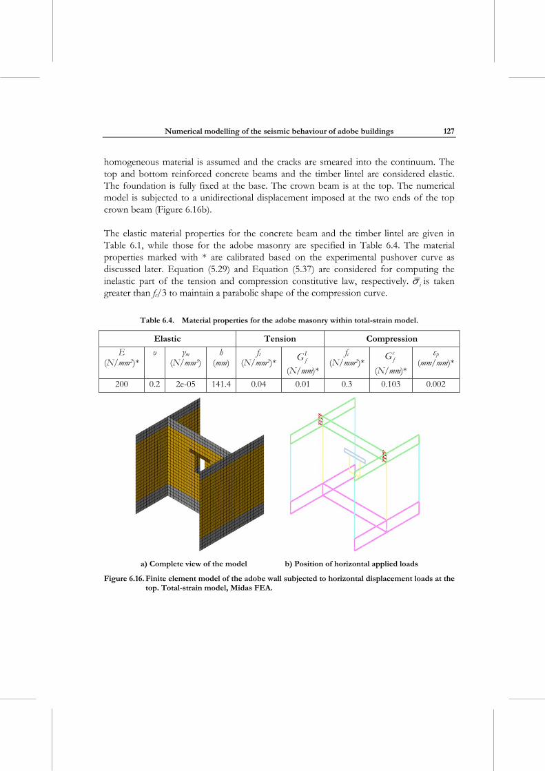
Numerical modelling of the seismic behaviour of adobe buildings
127
homogeneous material is assumed and the cracks are smeared into the continuum. The top and bottom reinforced concrete beams and the timber lintel are considered elastic. The foundation is fully fixed at the base. The crown beam is at the top. The numerical model is subjected to a unidirectional displacement imposed at the two ends of the top crown beam (Figure 6.16b).
The elastic material properties for the concrete beam and the timber lintel are given in Table 6.1, while those for the adobe masonry are specified in Table 6.4. The material properties marked with * are calibrated based on the experimental pushover curve as discussed later. Equation (5.29) and Equation (5.37) are considered for computing the inelastic part of the tension and compression constitutive law, respectively. i is taken greater than fc/3 to maintain a parabolic shape of the compression curve.
Table 6.4. Material properties for the adobe masonry within total-strain model.
Elastic Tension Compression
E (N/mm2)*
υ γm
(N/mm3) h
(mm)ft
(N/mm2)*IfG
(N/mm)*
fc (N/mm2)*
cfG
(N/mm)*
εp (mm/mm)*
200 0.2 2e-05 141.4 0.04 0.01 0.3 0.103 0.002
a) Complete view of the model b) Position of horizontal applied loads
Figure 6.16. Finite element model of the adobe wall subjected to horizontal displacement loads at the top. Total-strain model, Midas FEA.
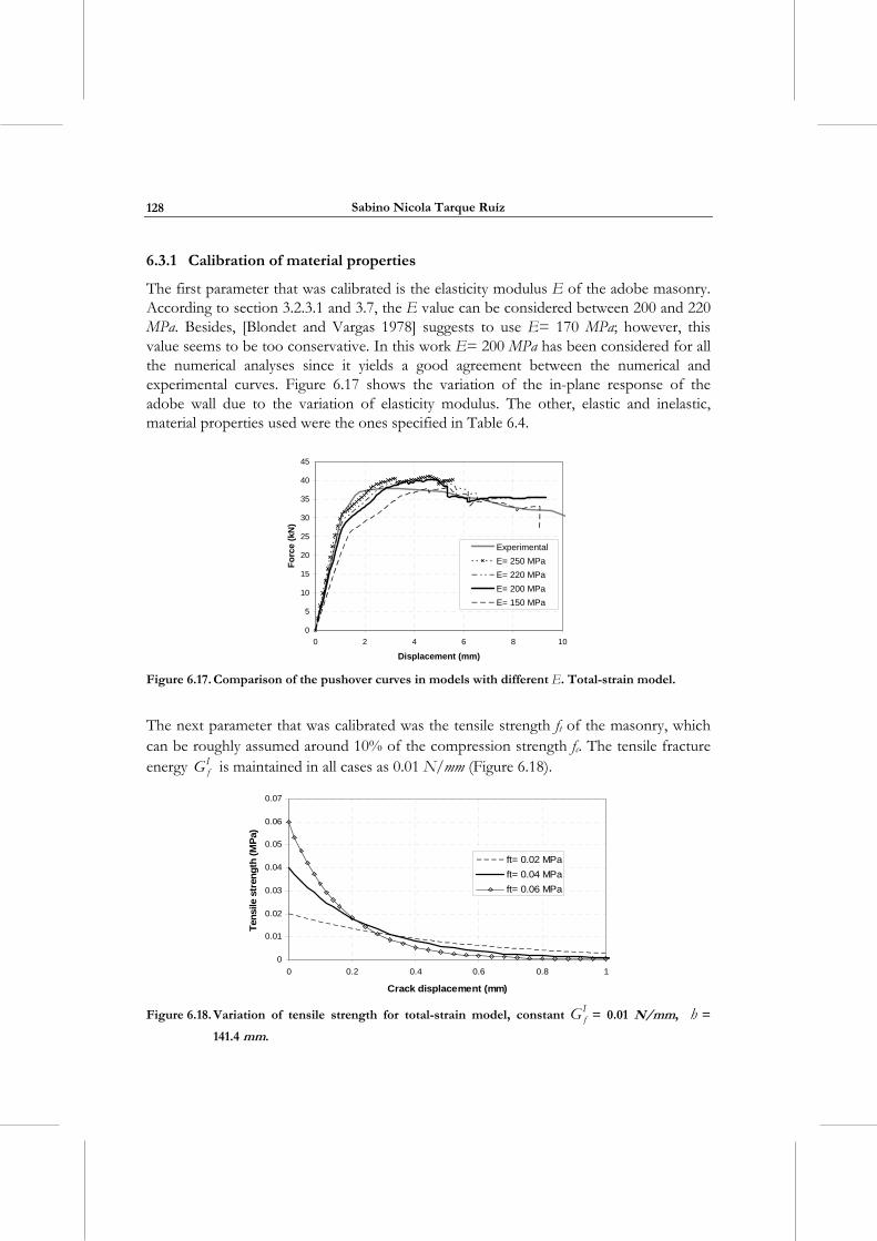
Sabino Nicola Tarque Ruíz
128
6.3.1 Calibration of material properties
The first parameter that was calibrated is the elasticity modulus E of the adobe masonry. According to section 3.2.3.1 and 3.7, the E value can be considered between 200 and 220 MPa. Besides, [Blondet and Vargas 1978] suggests to use E= 170 MPa; however, this value seems to be too conservative. In this work E= 200 MPa has been considered for all the numerical analyses since it yields a good agreement between the numerical and experimental curves. Figure 6.17 shows the variation of the in-plane response of the adobe wall due to the variation of elasticity modulus. The other, elastic and inelastic, material properties used were the ones specified in Table 6.4.
0
5
10
15
20
25
30
35
40
45
0 2 4 6 8 10
Displacement (mm)
Fo
rce
(kN
)
Experimental
E= 250 MPa
E= 220 MPa
E= 200 MPa
E= 150 MPa
Figure 6.17. Comparison of the pushover curves in models with different E. Total-strain model.
The next parameter that was calibrated was the tensile strength ft of the masonry, which can be roughly assumed around 10% of the compression strength fc. The tensile fracture energy I
fG is maintained in all cases as 0.01 N/mm (Figure 6.18).
0
0.01
0.02
0.03
0.04
0.05
0.06
0.07
0 0.2 0.4 0.6 0.8 1
Crack displacement (mm)
Ten
sile
str
eng
th (
MP
a)
ft= 0.02 MPa
ft= 0.04 MPa
ft= 0.06 MPa
Figure 6.18. Variation of tensile strength for total-strain model, constant I
fG = 0.01 N/mm, h =
141.4 mm.
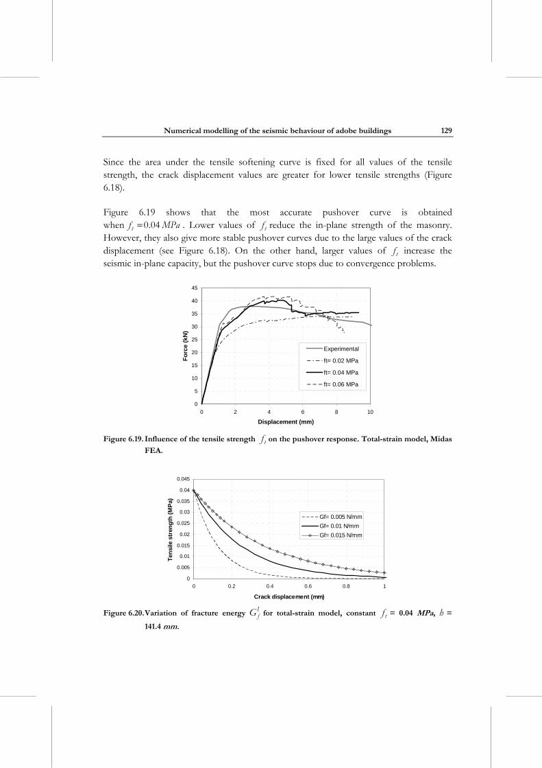
Numerical modelling of the seismic behaviour of adobe buildings
129
Since the area under the tensile softening curve is fixed for all values of the tensile strength, the crack displacement values are greater for lower tensile strengths (Figure 6.18).
Figure 6.19 shows that the most accurate pushover curve is obtained when tf MPa0.04 . Lower values of tf reduce the in-plane strength of the masonry. However, they also give more stable pushover curves due to the large values of the crack displacement (see Figure 6.18). On the other hand, larger values of tf increase the seismic in-plane capacity, but the pushover curve stops due to convergence problems.
0
5
10
15
20
25
30
35
40
45
0 2 4 6 8 10
Displacement (mm)
Fo
rce
(kN
)
Experimental
ft= 0.02 MPa
ft= 0.04 MPa
ft= 0.06 MPa
Figure 6.19. Influence of the tensile strength tf on the pushover response. Total-strain model, Midas
FEA.
0
0.005
0.01
0.015
0.02
0.025
0.03
0.035
0.04
0.045
0 0.2 0.4 0.6 0.8 1
Crack displacement (mm)
Ten
sile
str
eng
th (
MP
a)
Gf= 0.005 N/mm
Gf= 0.01 N/mm
Gf= 0.015 N/mm
Figure 6.20. Variation of fracture energy I
fG for total-strain model, constant tf = 0.04 MPa, h =
141.4 mm.
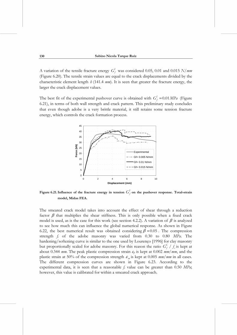
Sabino Nicola Tarque Ruíz
130
A variation of the tensile fracture energy IfG was considered 0.05, 0.01 and 0.015 N/mm
(Figure 6.20). The tensile strain values are equal to the crack displacements divided by the characteristic element length h (141.4 mm). It is seen that greater the fracture energy, the larger the crack displacement values.
The best fit of the experimental pushover curve is obtained with IfG MPa0.01 (Figure
6.21), in terms of both wall strength and crack pattern. This preliminary study concludes that even though adobe is a very brittle material, it still retains some tension fracture energy, which controls the crack formation process.
0
5
10
15
20
25
30
35
40
45
0 2 4 6 8 10
Displacement (mm)
Fo
rce
(kN
)
Experimental
Gf= 0.005 N/mm
Gf= 0.01 N/mm
Gf= 0.015 N/mm
Figure 6.21. Influence of the fracture energy in tension IfG on the pushover response. Total-strain
model, Midas FEA.
The smeared crack model takes into account the effect of shear through a reduction factor that multiplies the shear stiffness. This is only possible when a fixed crack model is used, as is the case for this work (see section 4.2.2). A variation of is analyzed to see how much this can influence the global numerical response. As shown in Figure 6.22, the best numerical result was obtained considering 0.05 . The compression strength fc of the adobe masonry was varied from 0.30 to 0.80 MPa. The hardening/softening curve is similar to the one used by Lourenço [1996] for clay masonry but proportionally scaled for adobe masonry. For this reason the ratio C
f cG f/ is kept at about 0.344 mm. The peak plastic compression strain p is kept at 0.002 mm/mm, and the plastic strain at 50% of the compression strength m is kept at 0.005 mm/mm in all cases. The different compression curves are shown in Figure 6.23. According to the experimental data, it is seen that a reasonable fc value can be greater than 0.50 MPa; however, this value is calibrated for within a smeared crack approach.
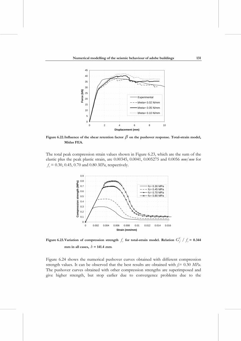
Numerical modelling of the seismic behaviour of adobe buildings
131
0
5
10
15
20
25
30
35
40
45
0 2 4 6 8 10
Displacement (mm)
Fo
rce
(kN
)
Experimental
bheta= 0.02 N/mm
bheta= 0.05 N/mm
bheta= 0.10 N/mm
Figure 6.22. Influence of the shear retention factor on the pushover response. Total-strain model,
Midas FEA.
The total peak compression strain values shown in Figure 6.23, which are the sum of the elastic plus the peak plastic strain, are 0.00345, 0.0041, 0.005275 and 0.0056 mm/mm for
cf = 0.30, 0.45, 0.70 and 0.80 MPa, respectively.
0
0.1
0.2
0.3
0.4
0.5
0.6
0.7
0.8
0.9
0 0.002 0.004 0.006 0.008 0.01 0.012 0.014 0.016
Strain (mm/mm)
Co
mp
res
sio
n s
tre
ng
th (
MP
a)
fc= 0.30 MPafc= 0.45 MPafc= 0.70 MPafc= 0.80 MPa
Figure 6.23. Variation of compression strength cf for total-strain model. Relation Cf cG f/ = 0.344
mm in all cases, h = 141.4 mm.
Figure 6.24 shows the numerical pushover curves obtained with different compression strength values. It can be observed that the best results are obtained with fc= 0.30 MPa. The pushover curves obtained with other compression strengths are superimposed and give higher strength, but stop earlier due to convergence problems due to the
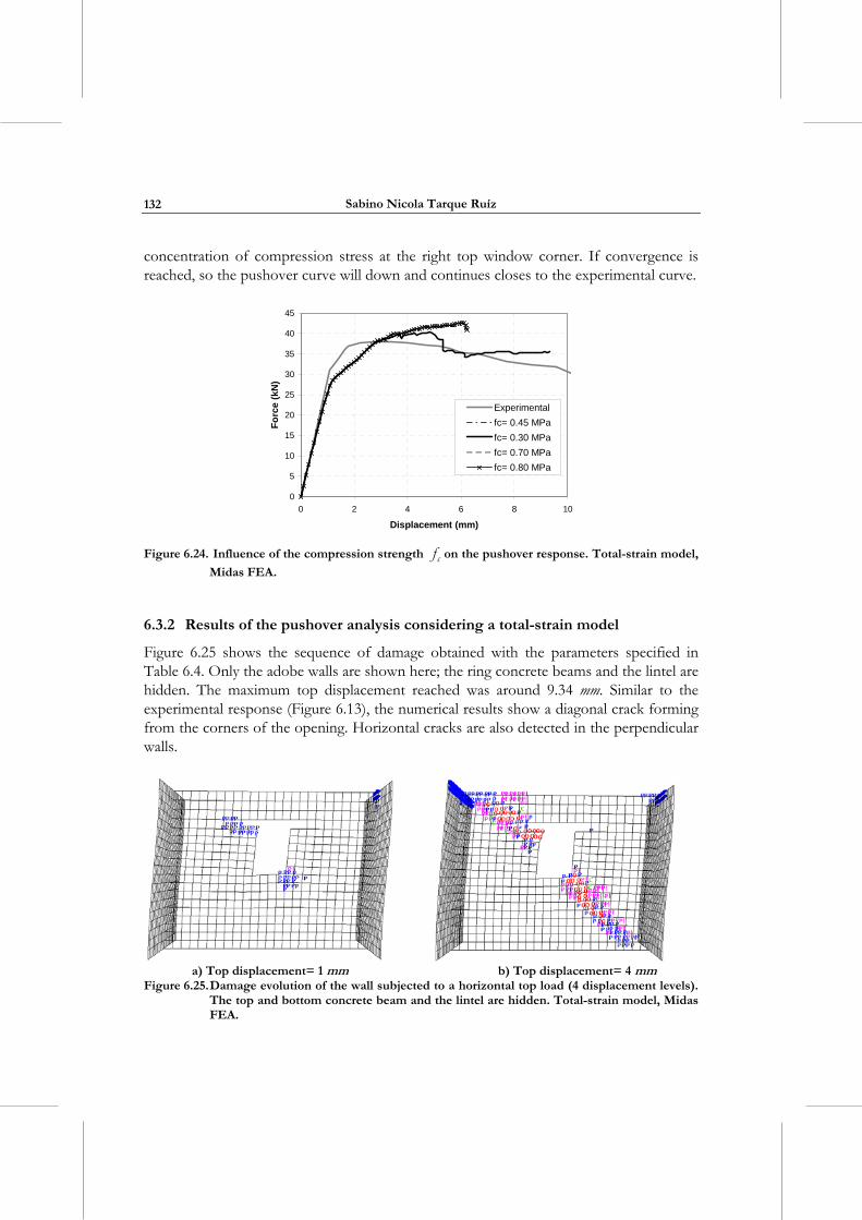
Sabino Nicola Tarque Ruíz
132
concentration of compression stress at the right top window corner. If convergence is reached, so the pushover curve will down and continues closes to the experimental curve.
0
5
10
15
20
25
30
35
40
45
0 2 4 6 8 10
Displacement (mm)
Fo
rce
(k
N)
Experimental
fc= 0.45 MPa
fc= 0.30 MPa
fc= 0.70 MPa
fc= 0.80 MPa
Figure 6.24. Influence of the compression strength cf on the pushover response. Total-strain model,
Midas FEA.
6.3.2 Results of the pushover analysis considering a total-strain model
Figure 6.25 shows the sequence of damage obtained with the parameters specified in Table 6.4. Only the adobe walls are shown here; the ring concrete beams and the lintel are hidden. The maximum top displacement reached was around 9.34 mm. Similar to the experimental response (Figure 6.13), the numerical results show a diagonal crack forming from the corners of the opening. Horizontal cracks are also detected in the perpendicular walls.
a) Top displacement= 1 mm b) Top displacement= 4 mm
Figure 6.25. Damage evolution of the wall subjected to a horizontal top load (4 displacement levels). The top and bottom concrete beam and the lintel are hidden. Total-strain model, Midas FEA.
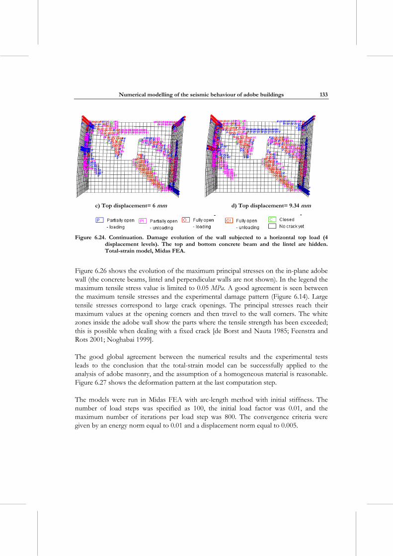
Numerical modelling of the seismic behaviour of adobe buildings
133
c) Top displacement= 6 mm d) Top displacement= 9.34 mm
Figure 6.24. Continuation. Damage evolution of the wall subjected to a horizontal top load (4
displacement levels). The top and bottom concrete beam and the lintel are hidden. Total-strain model, Midas FEA.
Figure 6.26 shows the evolution of the maximum principal stresses on the in-plane adobe wall (the concrete beams, lintel and perpendicular walls are not shown). In the legend the maximum tensile stress value is limited to 0.05 MPa. A good agreement is seen between the maximum tensile stresses and the experimental damage pattern (Figure 6.14). Large tensile stresses correspond to large crack openings. The principal stresses reach their maximum values at the opening corners and then travel to the wall corners. The white zones inside the adobe wall show the parts where the tensile strength has been exceeded; this is possible when dealing with a fixed crack [de Borst and Nauta 1985; Feenstra and Rots 2001; Noghabai 1999].
The good global agreement between the numerical results and the experimental tests leads to the conclusion that the total-strain model can be successfully applied to the analysis of adobe masonry, and the assumption of a homogeneous material is reasonable. Figure 6.27 shows the deformation pattern at the last computation step.
The models were run in Midas FEA with arc-length method with initial stiffness. The number of load steps was specified as 100, the initial load factor was 0.01, and the maximum number of iterations per load step was 800. The convergence criteria were given by an energy norm equal to 0.01 and a displacement norm equal to 0.005.
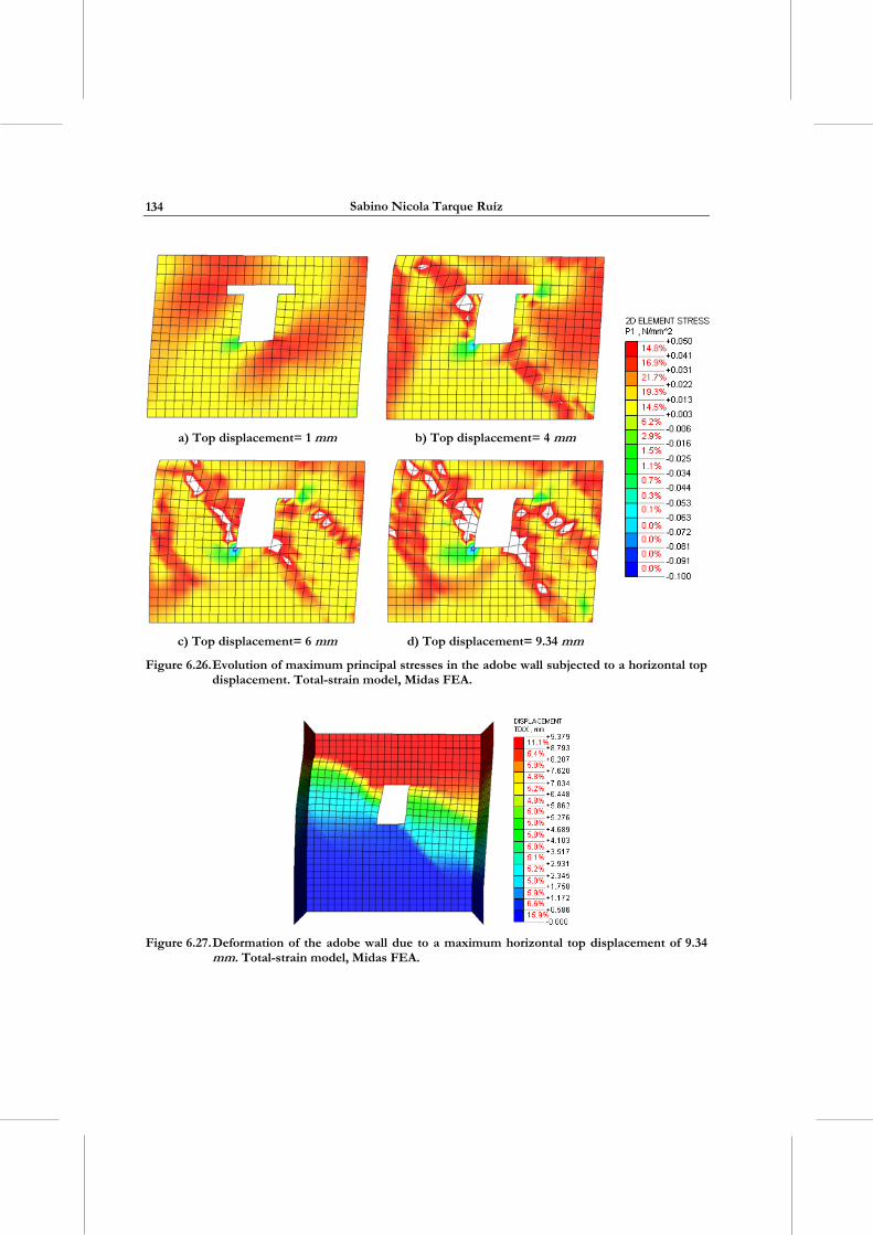
Sabino Nicola Tarque Ruíz
134
a) Top displacement= 1 mm b) Top displacement= 4 mm
c) Top displacement= 6 mm d) Top displacement= 9.34 mm
Figure 6.26. Evolution of maximum principal stresses in the adobe wall subjected to a horizontal top displacement. Total-strain model, Midas FEA.
Figure 6.27. Deformation of the adobe wall due to a maximum horizontal top displacement of 9.34
mm. Total-strain model, Midas FEA.
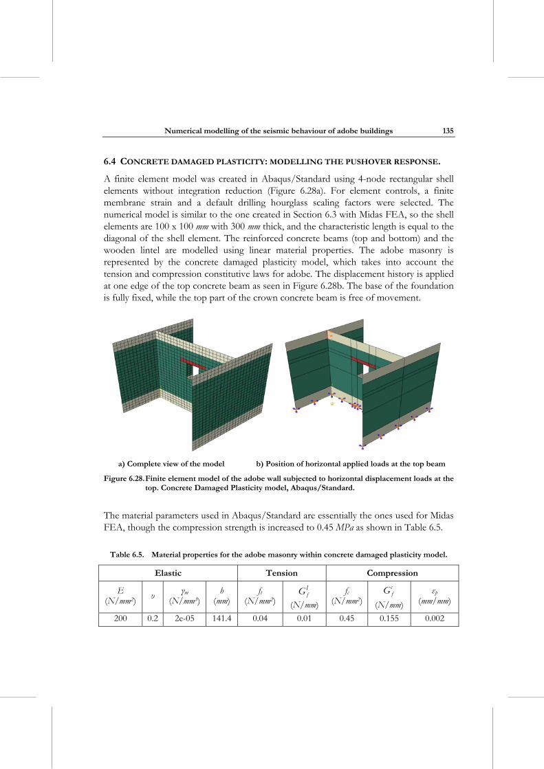
Numerical modelling of the seismic behaviour of adobe buildings
135
6.4 CONCRETE DAMAGED PLASTICITY: MODELLING THE PUSHOVER RESPONSE.
A finite element model was created in Abaqus/Standard using 4-node rectangular shell elements without integration reduction (Figure 6.28a). For element controls, a finite membrane strain and a default drilling hourglass scaling factors were selected. The numerical model is similar to the one created in Section 6.3 with Midas FEA, so the shell elements are 100 x 100 mm with 300 mm thick, and the characteristic length is equal to the diagonal of the shell element. The reinforced concrete beams (top and bottom) and the wooden lintel are modelled using linear material properties. The adobe masonry is represented by the concrete damaged plasticity model, which takes into account the tension and compression constitutive laws for adobe. The displacement history is applied at one edge of the top concrete beam as seen in Figure 6.28b. The base of the foundation is fully fixed, while the top part of the crown concrete beam is free of movement.
a) Complete view of the model b) Position of horizontal applied loads at the top beam
Figure 6.28. Finite element model of the adobe wall subjected to horizontal displacement loads at the top. Concrete Damaged Plasticity model, Abaqus/Standard.
The material parameters used in Abaqus/Standard are essentially the ones used for Midas FEA, though the compression strength is increased to 0.45 MPa as shown in Table 6.5.
Table 6.5. Material properties for the adobe masonry within concrete damaged plasticity model.
Elastic Tension Compression
E (N/mm2)
υ γm
(N/mm3) h
(mm) ft
(N/mm2)
IfG
(N/mm)
fc (N/mm2)
cfG
(N/mm)
εp (mm/mm)
200 0.2 2e-05 141.4 0.04 0.01 0.45 0.155 0.002
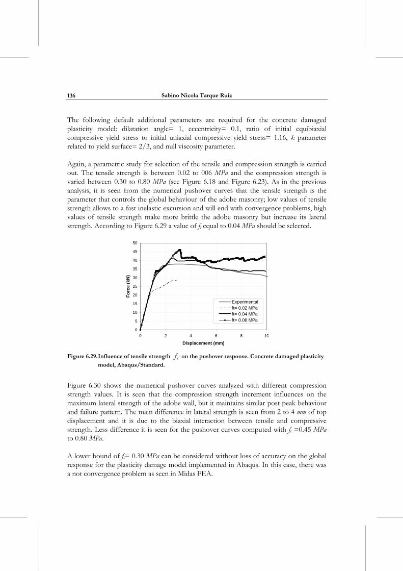
Sabino Nicola Tarque Ruíz
136
The following default additional parameters are required for the concrete damaged plasticity model: dilatation angle= 1, eccentricity= 0.1, ratio of initial equibiaxial compressive yield stress to initial uniaxial compressive yield stress= 1.16, k parameter related to yield surface= 2/3, and null viscosity parameter.
Again, a parametric study for selection of the tensile and compression strength is carried out. The tensile strength is between 0.02 to 006 MPa and the compression strength is varied between 0.30 to 0.80 MPa (see Figure 6.18 and Figure 6.23). As in the previous analysis, it is seen from the numerical pushover curves that the tensile strength is the parameter that controls the global behaviour of the adobe masonry; low values of tensile strength allows to a fast inelastic excursion and will end with convergence problems, high values of tensile strength make more brittle the adobe masonry but increase its lateral strength. According to Figure 6.29 a value of ft equal to 0.04 MPa should be selected.
0
5
10
15
20
25
30
35
40
45
50
0 2 4 6 8 10
Displacement (mm)
Fo
rce
(kN
)
Experimentalft= 0.02 MPaft= 0.04 MPaft= 0.06 MPa
Figure 6.29. Influence of tensile strength tf on the pushover response. Concrete damaged plasticity
model, Abaqus/Standard.
Figure 6.30 shows the numerical pushover curves analyzed with different compression strength values. It is seen that the compression strength increment influences on the maximum lateral strength of the adobe wall, but it maintains similar post peak behaviour and failure pattern. The main difference in lateral strength is seen from 2 to 4 mm of top displacement and it is due to the biaxial interaction between tensile and compressive strength. Less difference it is seen for the pushover curves computed with fc =0.45 MPa to 0.80 MPa.
A lower bound of fc= 0.30 MPa can be considered without loss of accuracy on the global response for the plasticity damage model implemented in Abaqus. In this case, there was a not convergence problem as seen in Midas FEA.
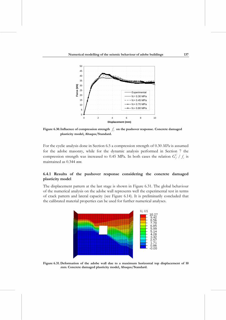
Numerical modelling of the seismic behaviour of adobe buildings
137
0
5
10
15
20
25
30
35
40
45
50
0 2 4 6 8 10
Displacement (mm)
Fo
rce
(kN
)
Experimental
fc= 0.30 MPa
fc= 0.45 MPa
fc= 0.70 MPa
fc= 0.80 MPa
Figure 6.30. Influence of compression strength cf on the pushover response. Concrete damaged
plasticity model, Abaqus/Standard.
For the cyclic analysis done in Section 6.5 a compression strength of 0.30 MPa is assumed for the adobe masonry, while for the dynamic analysis performed in Section 7 the compression strength was increased to 0.45 MPa. In both cases the relation C
f cG f/ is maintained as 0.344 mm.
6.4.1 Results of the pushover response considering the concrete damaged plasticity model
The displacement pattern at the last stage is shown in Figure 6.31. The global behaviour of the numerical analysis on the adobe wall represents well the experimental test in terms of crack pattern and lateral capacity (see Figure 6.14). It is preliminarily concluded that the calibrated material properties can be used for further numerical analyses.
Figure 6.31. Deformation of the adobe wall due to a maximum horizontal top displacement of 10
mm. Concrete damaged plasticity model, Abaqus/Standard.
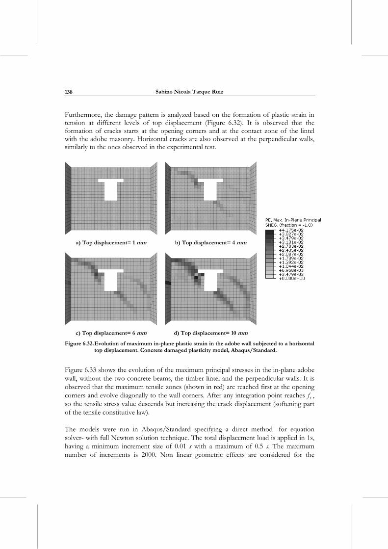
Sabino Nicola Tarque Ruíz
138
Furthermore, the damage pattern is analyzed based on the formation of plastic strain in tension at different levels of top displacement (Figure 6.32). It is observed that the formation of cracks starts at the opening corners and at the contact zone of the lintel with the adobe masonry. Horizontal cracks are also observed at the perpendicular walls, similarly to the ones observed in the experimental test.
a) Top displacement= 1 mm b) Top displacement= 4 mm
c) Top displacement= 6 mm d) Top displacement= 10 mm
Figure 6.32. Evolution of maximum in-plane plastic strain in the adobe wall subjected to a horizontal top displacement. Concrete damaged plasticity model, Abaqus/Standard.
Figure 6.33 shows the evolution of the maximum principal stresses in the in-plane adobe wall, without the two concrete beams, the timber lintel and the perpendicular walls. It is observed that the maximum tensile zones (shown in red) are reached first at the opening corners and evolve diagonally to the wall corners. After any integration point reaches tf , so the tensile stress value descends but increasing the crack displacement (softening part of the tensile constitutive law).
The models were run in Abaqus/Standard specifying a direct method -for equation solver- with full Newton solution technique. The total displacement load is applied in 1s, having a minimum increment size of 0.01 s with a maximum of 0.5 s. The maximum number of increments is 2000. Non linear geometric effects are considered for the
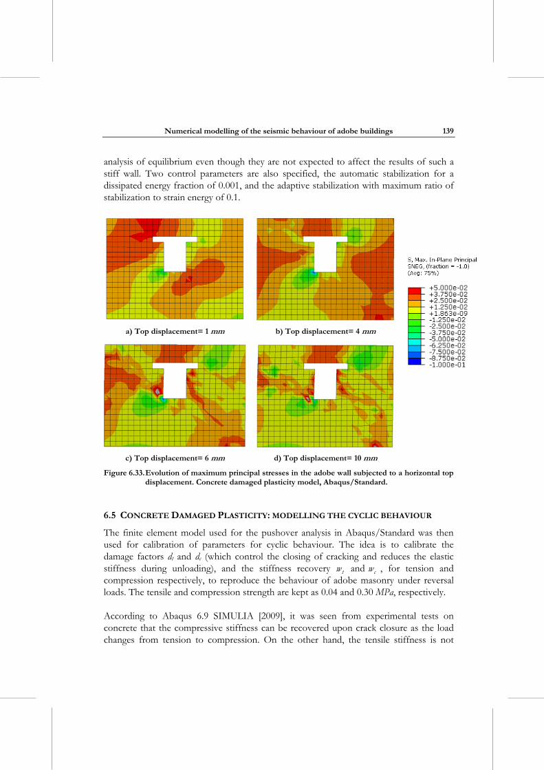
Numerical modelling of the seismic behaviour of adobe buildings
139
analysis of equilibrium even though they are not expected to affect the results of such a stiff wall. Two control parameters are also specified, the automatic stabilization for a dissipated energy fraction of 0.001, and the adaptive stabilization with maximum ratio of stabilization to strain energy of 0.1.
a) Top displacement= 1 mm b) Top displacement= 4 mm
c) Top displacement= 6 mm d) Top displacement= 10 mm
Figure 6.33. Evolution of maximum principal stresses in the adobe wall subjected to a horizontal top displacement. Concrete damaged plasticity model, Abaqus/Standard.
6.5 CONCRETE DAMAGED PLASTICITY: MODELLING THE CYCLIC BEHAVIOUR
The finite element model used for the pushover analysis in Abaqus/Standard was then used for calibration of parameters for cyclic behaviour. The idea is to calibrate the damage factors dt and dc (which control the closing of cracking and reduces the elastic stiffness during unloading), and the stiffness recovery tw and cw , for tension and compression respectively, to reproduce the behaviour of adobe masonry under reversal loads. The tensile and compression strength are kept as 0.04 and 0.30 MPa, respectively.
According to Abaqus 6.9 SIMULIA [2009], it was seen from experimental tests on concrete that the compressive stiffness can be recovered upon crack closure as the load changes from tension to compression. On the other hand, the tensile stiffness is not
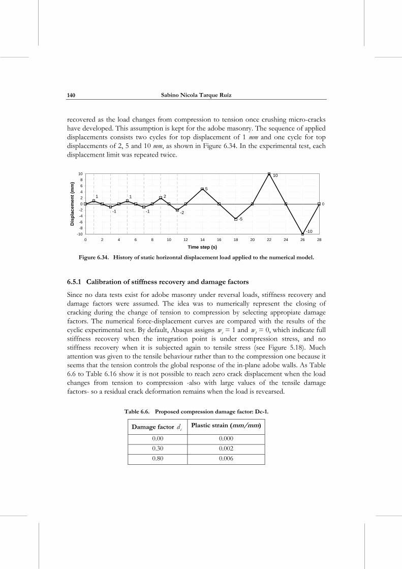
Sabino Nicola Tarque Ruíz
140
recovered as the load changes from compression to tension once crushing micro-cracks have developed. This assumption is kept for the adobe masonry. The sequence of applied displacements consists two cycles for top displacement of 1 mm and one cycle for top displacements of 2, 5 and 10 mm, as shown in Figure 6.34. In the experimental test, each displacement limit was repeated twice.
2
-2
0
1
-1
1
-1
-10
10
-5
5
-10
-8
-6
-4
-2
0
2
4
6
8
10
0 2 4 6 8 10 12 14 16 18 20 22 24 26 28
Time step (s)
Dis
pla
cem
ent
(mm
)
Figure 6.34. History of static horizontal displacement load applied to the numerical model.
6.5.1 Calibration of stiffness recovery and damage factors
Since no data tests exist for adobe masonry under reversal loads, stiffness recovery and damage factors were assumed. The idea was to numerically represent the closing of cracking during the change of tension to compression by selecting appropiate damage factors. The numerical force-displacement curves are compared with the results of the cyclic experimental test. By default, Abaqus assigns cw = 1 and tw = 0, which indicate full stiffness recovery when the integration point is under compression stress, and no stiffness recovery when it is subjected again to tensile stress (see Figure 5.18). Much attention was given to the tensile behaviour rather than to the compression one because it seems that the tension controls the global response of the in-plane adobe walls. As Table 6.6 to Table 6.16 show it is not possible to reach zero crack displacement when the load changes from tension to compression -also with large values of the tensile damage factors- so a residual crack deformation remains when the load is revearsed.
Table 6.6. Proposed compression damage factor: Dc-1.
Damage factor cd Plastic strain (mm/mm)
0.00 0.000
0.30 0.002
0.80 0.006
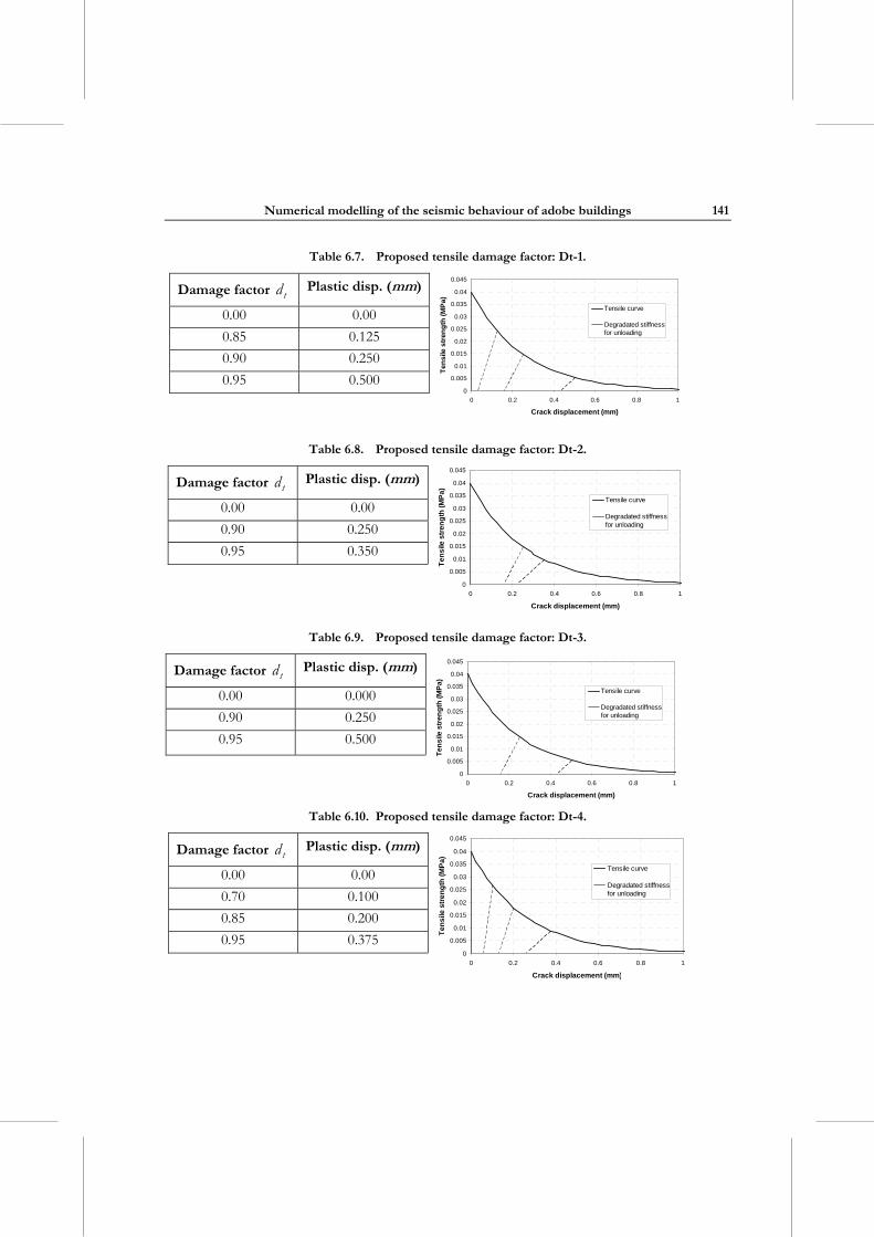
Numerical modelling of the seismic behaviour of adobe buildings
141
Table 6.7. Proposed tensile damage factor: Dt-1.
Damage factor td Plastic disp. (mm)
0.00 0.00
0.85 0.125
0.90 0.250
0.95 0.500
0
0.005
0.01
0.015
0.02
0.025
0.03
0.035
0.04
0.045
0 0.2 0.4 0.6 0.8 1
Crack displacement (mm)
Te
ns
ile s
tren
gth
(M
Pa
)
Tensile curve
Degradated stiffnessfor unloading
Table 6.8. Proposed tensile damage factor: Dt-2.
Damage factor td Plastic disp. (mm)
0.00 0.00
0.90 0.250
0.95 0.350
0
0.005
0.01
0.015
0.02
0.025
0.03
0.035
0.04
0.045
0 0.2 0.4 0.6 0.8 1
Crack displacement (mm)
Te
ns
ile s
tre
ng
th (
MP
a)
Tensile curve
Degradated stiffnessfor unloading
Table 6.9. Proposed tensile damage factor: Dt-3.
Damage factor td Plastic disp. (mm)
0.00 0.000
0.90 0.250
0.95 0.500
0
0.005
0.01
0.015
0.02
0.025
0.03
0.035
0.04
0.045
0 0.2 0.4 0.6 0.8 1
Crack displacement (mm)
Te
ns
ile s
tre
ng
th (
MP
a)
Tensile curve
Degradated stiffnessfor unloading
Table 6.10. Proposed tensile damage factor: Dt-4.
Damage factor td Plastic disp. (mm)
0.00 0.00
0.70 0.100
0.85 0.200
0.95 0.375
0
0.005
0.01
0.015
0.02
0.025
0.03
0.035
0.04
0.045
0 0.2 0.4 0.6 0.8 1
Crack displacement (mm)
Ten
sile
str
en
gth
(M
Pa)
Tensile curve
Degradated stiffnessfor unloading
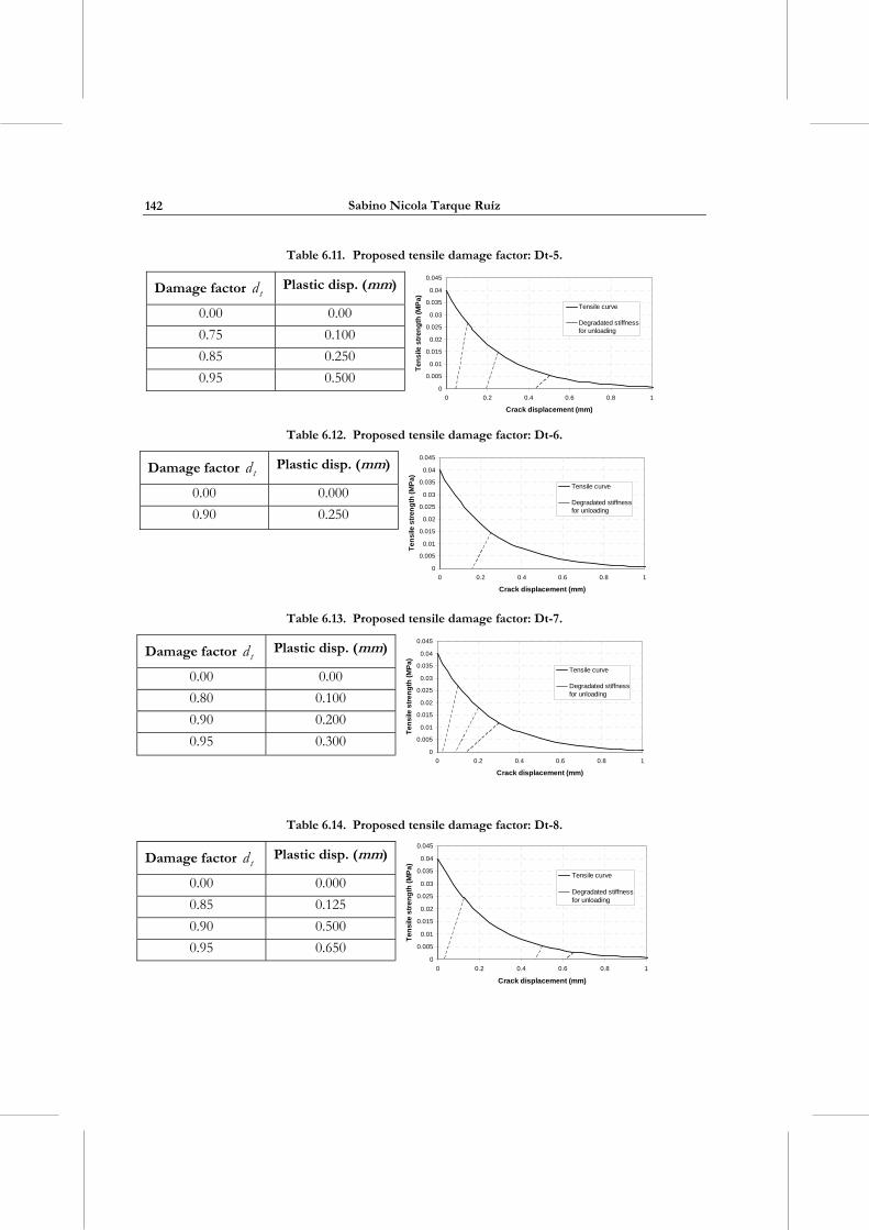
Sabino Nicola Tarque Ruíz
142
Table 6.11. Proposed tensile damage factor: Dt-5.
Damage factor td Plastic disp. (mm)
0.00 0.00
0.75 0.100
0.85 0.250
0.95 0.500
0
0.005
0.01
0.015
0.02
0.025
0.03
0.035
0.04
0.045
0 0.2 0.4 0.6 0.8 1
Crack displacement (mm)T
en
sile
str
eng
th (
MP
a)
Tensile curve
Degradated stiffnessfor unloading
Table 6.12. Proposed tensile damage factor: Dt-6.
Damage factor td Plastic disp. (mm)
0.00 0.000
0.90 0.250
0
0.005
0.01
0.015
0.02
0.025
0.03
0.035
0.04
0.045
0 0.2 0.4 0.6 0.8 1
Crack displacement (mm)
Te
ns
ile s
tren
gth
(M
Pa
)
Tensile curve
Degradated stiffnessfor unloading
Table 6.13. Proposed tensile damage factor: Dt-7.
Damage factor td Plastic disp. (mm)
0.00 0.00
0.80 0.100
0.90 0.200
0.95 0.300
0
0.005
0.01
0.015
0.02
0.025
0.03
0.035
0.04
0.045
0 0.2 0.4 0.6 0.8 1
Crack displacement (mm)
Ten
sile
str
en
gth
(M
Pa
)
Tensile curve
Degradated stiffnessfor unloading
Table 6.14. Proposed tensile damage factor: Dt-8.
Damage factor td Plastic disp. (mm)
0.00 0.000
0.85 0.125
0.90 0.500
0.95 0.650
0
0.005
0.01
0.015
0.02
0.025
0.03
0.035
0.04
0.045
0 0.2 0.4 0.6 0.8 1
Crack displacement (mm)
Te
ns
ile s
tre
ng
th (
MP
a)
Tensile curve
Degradated stiffnessfor unloading
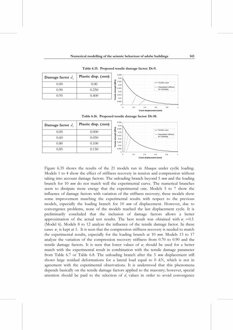
Numerical modelling of the seismic behaviour of adobe buildings
143
Table 6.15. Proposed tensile damage factor: Dt-9.
Damage factor td Plastic disp. (mm)
0.00 0.00
0.90 0.250
0.95 0.400
0
0.005
0.01
0.015
0.02
0.025
0.03
0.035
0.04
0.045
0 0.2 0.4 0.6 0.8 1
Crack displacement (mm)
Te
ns
ile s
tre
ng
th (
MP
a)
Tensile curve
Degradated stiffnessfor unloading
Table 6.16. Proposed tensile damage factor: Dt-10.
Damage factor td Plastic disp. (mm)
0.00 0.000
0.60 0.050
0.80 0.100
0.85 0.150
0
0.005
0.01
0.015
0.02
0.025
0.03
0.035
0.04
0.045
0 0.2 0.4 0.6 0.8 1
Crack displacement (mm)
Te
ns
ile s
tren
gth
(M
Pa
)
Tensile curve
Degradated stiffnessfor unloading
Figure 6.35 shows the results of the 21 models run in Abaqus under cyclic loading. Models 1 to 4 show the effect of stiffness recovery in tension and compression without taking into account damage factors. The unloading branch beyond 5 mm and the loading branch for 10 mm do not match well the experimental curve. The numerical branches seem to dissipate more energy that the experimental one. Models 5 to 7 show the influence of damage factors with variation of the stiffness recovery; these models show some improvement matching the experimental results with respect to the previous models, especially the loading branch for 10 mm of displacement. However, due to convergence problems, none of the models reached the last displacement cycle. It is preliminarily concluded that the inclusion of damage factors allows a better approximation of the actual test results. The best result was obtained with cw 0.5 (Model 6). Models 8 to 12 analyze the influence of the tensile damage factor. In these cases cw is kept at 1. It is seen that the compression stiffness recovery is needed to match the experimental results, especially for the loading branch at 10 mm. Models 13 to 17 analyze the variation of the compression recovery stiffness from 0.70 to 0.90 and the tensile damage factors. It is seen that lower values of cw should be used for a better match with the experimental result in combination with the tensile damage parameter from Table 6.7 or Table 6.8. The unloading branch after the 5 mm displacement still shows large residual deformations for a lateral load equal to 0 kN, which is not in agreement with the experimental observations. It is understood that this phenomena depends basically on the tensile damage factors applied to the masonry; however, special attention should be paid to the selection of td values in order to avoid convergence
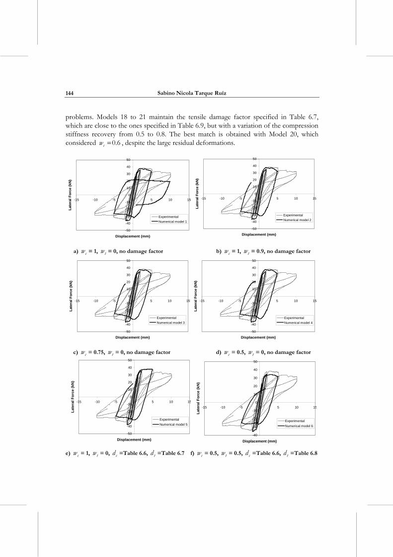
Sabino Nicola Tarque Ruíz
144
problems. Models 18 to 21 maintain the tensile damage factor specified in Table 6.7, which are close to the ones specified in Table 6.9, but with a variation of the compression stiffness recovery from 0.5 to 0.8. The best match is obtained with Model 20, which considered cw 0.6 , despite the large residual deformations.
-50
-40
-30
-20
-10
0
10
20
30
40
50
-15 -10 -5 0 5 10 15
Displacement (mm)
Lat
eral
Fo
rce
(kN
)
Experimental
Numerical model 1
-50
-40
-30
-20
-10
0
10
20
30
40
50
-15 -10 -5 0 5 10 15
Displacement (mm)
Lat
eral
Fo
rce
(kN
)
Experimental
Numerical model 2
a) cw = 1, tw = 0, no damage factor b) cw = 1, tw = 0.9, no damage factor
-50
-40
-30
-20
-10
0
10
20
30
40
50
-15 -10 -5 0 5 10 15
Displacement (mm)
Lat
era
l F
orc
e (k
N)
Experimental
Numerical model 3
-50
-40
-30
-20
-10
0
10
20
30
40
50
-15 -10 -5 0 5 10 15
Displacement (mm)
Lat
era
l F
orc
e (k
N)
Experimental
Numerical model 4
c) cw = 0.75, tw = 0, no damage factor d) cw = 0.5, tw = 0, no damage factor
-50
-40
-30
-20
-10
0
10
20
30
40
50
-15 -10 -5 0 5 10 15
Displacement (mm)
Lat
era
l F
orc
e (
kN)
Experimental
Numerical model 5
-40
-30
-20
-10
0
10
20
30
40
50
-15 -10 -5 0 5 10 15
Displacement (mm)
Lat
era
l Fo
rce
(k
N)
Experimental
Numerical model 6
e) cw = 1, tw = 0, cd =Table 6.6, td =Table 6.7 f) cw = 0.5, tw = 0.5, cd =Table 6.6, td =Table 6.8
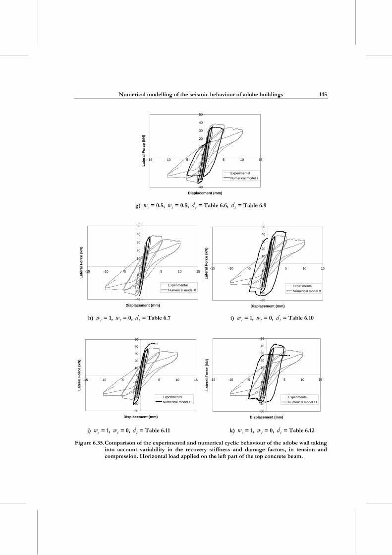
Numerical modelling of the seismic behaviour of adobe buildings
145
-40
-30
-20
-10
0
10
20
30
40
50
-15 -10 -5 0 5 10 15
Displacement (mm)
Lat
eral
Fo
rce
(kN
)
Experimental
Numerical model 7
g) cw = 0.5, tw = 0.5, cd = Table 6.6, td = Table 6.9
-40
-30
-20
-10
0
10
20
30
40
50
-15 -10 -5 0 5 10 15
Displacement (mm)
Lat
era
l F
orc
e (
kN
)
Experimental
Numerical model 8
-50
-40
-30
-20
-10
0
10
20
30
40
50
-15 -10 -5 0 5 10 15
Displacement (mm)
La
tera
l F
orc
e (k
N)
Experimental
Numerical model 9
h) cw = 1, tw = 0, td = Table 6.7 i) cw = 1, tw = 0, td = Table 6.10
-50
-40
-30
-20
-10
0
10
20
30
40
50
-15 -10 -5 0 5 10 15
Displacement (mm)
Lat
eral
Fo
rce
(kN
)
Experimental
Numerical model 10
-50
-40
-30
-20
-10
0
10
20
30
40
50
-15 -10 -5 0 5 10 15
Displacement (mm)
Lat
eral
Fo
rce
(kN
)
Experimental
Numerical model 11
j) cw = 1, tw = 0, td = Table 6.11 k) cw = 1, tw = 0, td = Table 6.12
Figure 6.35. Comparison of the experimental and numerical cyclic behaviour of the adobe wall taking into account variability in the recovery stiffness and damage factors, in tension and compression. Horizontal load applied on the left part of the top concrete beam.
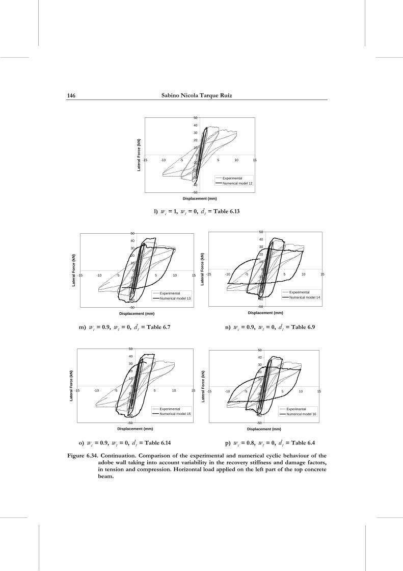
Sabino Nicola Tarque Ruíz
146
-50
-40
-30
-20
-10
0
10
20
30
40
50
-15 -10 -5 0 5 10 15
Displacement (mm)
Lat
eral
Fo
rce
(kN
)
Experimental
Numerical model 12
l) cw = 1, tw = 0, td = Table 6.13
-50
-40
-30
-20
-10
0
10
20
30
40
50
-15 -10 -5 0 5 10 15
Displacement (mm)
Lat
eral
Fo
rce
(kN
)
Experimental
Numerical model 13
-50
-40
-30
-20
-10
0
10
20
30
40
50
-15 -10 -5 0 5 10 15
Displacement (mm)
Lat
era
l F
orc
e (k
N)
Experimental
Numerical model 14
m) cw = 0.9, tw = 0, td = Table 6.7 n) cw = 0.9, tw = 0, td = Table 6.9
-50
-40
-30
-20
-10
0
10
20
30
40
50
-15 -10 -5 0 5 10 15
Displacement (mm)
Lat
eral
Fo
rce
(kN
)
Experimental
Numerical model 15
-50
-40
-30
-20
-10
0
10
20
30
40
50
-15 -10 -5 0 5 10 15
Displacement (mm)
La
tera
l Fo
rce
(kN
)
Experimental
Numerical model 16
o) cw = 0.9, tw = 0, td = Table 6.14 p) cw = 0.8, tw = 0, td = Table 6.4
Figure 6.34. Continuation. Comparison of the experimental and numerical cyclic behaviour of the adobe wall taking into account variability in the recovery stiffness and damage factors, in tension and compression. Horizontal load applied on the left part of the top concrete beam.
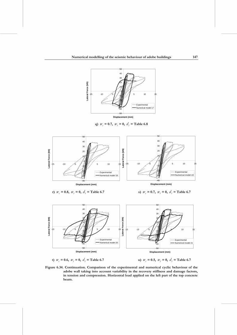
Numerical modelling of the seismic behaviour of adobe buildings
147
-50
-40
-30
-20
-10
0
10
20
30
40
50
-15 -10 -5 0 5 10 15
Displacement (mm)
Lat
era
l F
orc
e (k
N)
Experimental
Numerical model 17
q) cw = 0.7, tw = 0, td = Table 6.8
-40
-30
-20
-10
0
10
20
30
40
50
-15 -10 -5 0 5 10 15
Displacement (mm)
Lat
era
l F
orc
e (
kN)
Experimental
Numerical model 18
-40
-30
-20
-10
0
10
20
30
40
50
-15 -10 -5 0 5 10 15
Displacement (mm)
Lat
eral
Fo
rce
(kN
)
Experimental
Numerical model 19
r) cw = 0.8, tw = 0, td = Table 6.7 s) cw = 0.7, tw = 0, td = Table 6.7
-50
-40
-30
-20
-10
0
10
20
30
40
50
-15 -10 -5 0 5 10 15
Displacement (mm)
Lat
eral
Fo
rce
(kN
)
Experimental
Numerical model 20
-50
-40
-30
-20
-10
0
10
20
30
40
50
-15 -10 -5 0 5 10 15
Displacement (mm)
Late
ral
Fo
rce
(kN
)
Experimental
Numerical model 21
t) cw = 0.6, tw = 0, td = Table 6.7 u) cw = 0.5, tw = 0, td = Table 6.7
Figure 6.34. Continuation. Comparison of the experimental and numerical cyclic behaviour of the adobe wall taking into account variability in the recovery stiffness and damage factors, in tension and compression. Horizontal load applied on the left part of the top concrete beam.
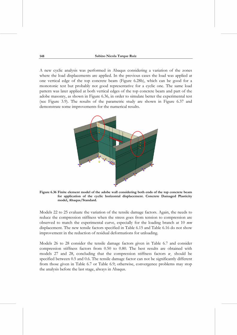
Sabino Nicola Tarque Ruíz
148
A new cyclic analysis was performed in Abaqus considering a variation of the zones where the load displacements are applied. In the previous cases the load was applied at one vertical edge of the top concrete beam (Figure 6.28b), which can be good for a monotonic test but probably not good representative for a cyclic one. The same load pattern was later applied at both vertical edges of the top concrete beam and part of the adobe masonry, as shown in Figure 6.36, in order to simulate better the experimental test (see Figure 3.9). The results of the parametric study are shown in Figure 6.37 and demonstrate some improvements for the numerical results.
Figure 6.36 Finite element model of the adobe wall considering both ends of the top concrete beam
for application of the cyclic horizontal displacement. Concrete Damaged Plasticity model, Abaqus/Standard.
Models 22 to 25 evaluate the variation of the tensile damage factors. Again, the needs to reduce the compression stiffness when the stress goes from tension to compression are observed to match the experimental curve, especially for the loading branch at 10 mm displacement. The new tensile factors specified in Table 6.15 and Table 6.16 do not show improvement in the reduction of residual deformations for unloading.
Models 26 to 28 consider the tensile damage factors given in Table 6.7 and consider compression stiffness factors from 0.50 to 0.80. The best results are obtained with models 27 and 28, concluding that the compression stiffness factors cw should be specified between 0.5 and 0.6. The tensile damage factor can not be significantly different from those given in Table 6.7 or Table 6.9; otherwise, convergence problems may stop the analysis before the last stage, always in Abaqus.
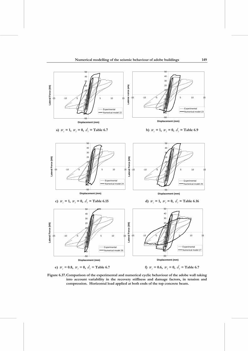
Numerical modelling of the seismic behaviour of adobe buildings
149
-50
-40
-30
-20
-10
0
10
20
30
40
50
-15 -10 -5 0 5 10 15
Displacement (mm)
Lat
eral
Fo
rce
(kN
)
Experimental
Numerical model 22
-50
-40
-30
-20
-10
0
10
20
30
40
50
-15 -10 -5 0 5 10 15
Displacement (mm)
Lat
era
l F
orc
e (k
N)
Experimental
Numerical model 23
a) cw = 1, tw = 0, td = Table 6.7 b) cw = 1, tw = 0, td = Table 6.9
-50
-40
-30
-20
-10
0
10
20
30
40
50
-15 -10 -5 0 5 10 15
Displacement (mm)
Lat
era
l F
orc
e (k
N)
Experimental
Numerical model 24
-50
-40
-30
-20
-10
0
10
20
30
40
50
-15 -10 -5 0 5 10 15
Displacement (mm)
Lat
eral
Fo
rce
(kN
)
Experimental
Numerical model 25
c) cw = 1, tw = 0, td = Table 6.15 d) cw = 1, tw = 0, td = Table 6.16
-50
-40
-30
-20
-10
0
10
20
30
40
50
-15 -10 -5 0 5 10 15
Displacement (mm)
Lat
era
l F
orc
e (k
N)
Experimental
Numerical model 26
-50
-40
-30
-20
-10
0
10
20
30
40
50
-15 -10 -5 0 5 10 15
Displacement (mm)
Lat
eral
Fo
rce
(kN
)
Experimental
Numerical model 27
e) cw = 0.8, tw = 0, td = Table 6.7 f) cw = 0.6, tw = 0, td = Table 6.7
Figure 6.37. Comparison of the experimental and numerical cyclic behaviour of the adobe wall taking into account variability in the recovery stiffness and damage factors, in tension and compression. Horizontal load applied at both ends of the top concrete beam.
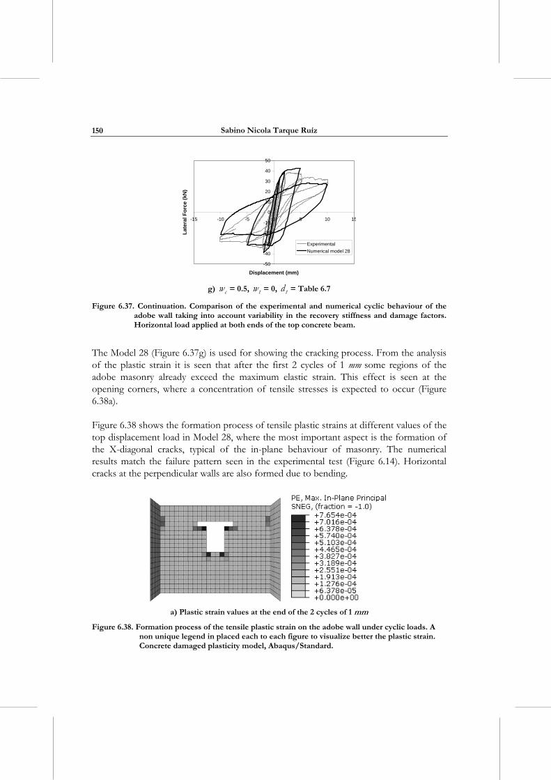
Sabino Nicola Tarque Ruíz
150
-50
-40
-30
-20
-10
0
10
20
30
40
50
-15 -10 -5 0 5 10 15
Displacement (mm)
Lat
eral
Fo
rce
(kN
)
Experimental
Numerical model 28
g) cw = 0.5, tw = 0, td = Table 6.7
Figure 6.37. Continuation. Comparison of the experimental and numerical cyclic behaviour of the adobe wall taking into account variability in the recovery stiffness and damage factors. Horizontal load applied at both ends of the top concrete beam.
The Model 28 (Figure 6.37g) is used for showing the cracking process. From the analysis of the plastic strain it is seen that after the first 2 cycles of 1 mm some regions of the adobe masonry already exceed the maximum elastic strain. This effect is seen at the opening corners, where a concentration of tensile stresses is expected to occur (Figure 6.38a).
Figure 6.38 shows the formation process of tensile plastic strains at different values of the top displacement load in Model 28, where the most important aspect is the formation of the X-diagonal cracks, typical of the in-plane behaviour of masonry. The numerical results match the failure pattern seen in the experimental test (Figure 6.14). Horizontal cracks at the perpendicular walls are also formed due to bending.
a) Plastic strain values at the end of the 2 cycles of 1 mm
Figure 6.38. Formation process of the tensile plastic strain on the adobe wall under cyclic loads. A non unique legend in placed each to each figure to visualize better the plastic strain. Concrete damaged plasticity model, Abaqus/Standard.
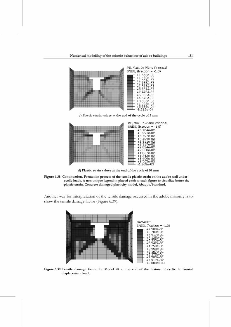
Numerical modelling of the seismic behaviour of adobe buildings
151
c) Plastic strain values at the end of the cycle of 5 mm
d) Plastic strain values at the end of the cycle of 10 mm
Figure 6.38. Continuation. Formation process of the tensile plastic strain on the adobe wall under cyclic loads. A non unique legend in placed each to each figure to visualize better the plastic strain. Concrete damaged plasticity model, Abaqus/Standard.
Another way for interpretation of the tensile damage occurred in the adobe masonry is to show the tensile damage factor (Figure 6.39).
Figure 6.39. Tensile damage factor for Model 28 at the end of the history of cyclic horizontal
displacement load.
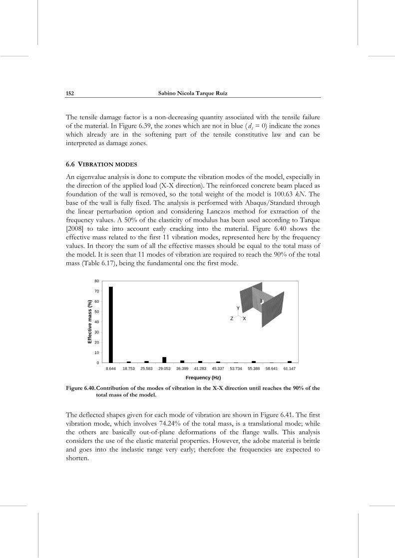
Sabino Nicola Tarque Ruíz
152
The tensile damage factor is a non-decreasing quantity associated with the tensile failure of the material. In Figure 6.39, the zones which are not in blue ( td = 0) indicate the zones which already are in the softening part of the tensile constitutive law and can be interpreted as damage zones.
6.6 VIBRATION MODES
An eigenvalue analysis is done to compute the vibration modes of the model, especially in the direction of the applied load (X-X direction). The reinforced concrete beam placed as foundation of the wall is removed, so the total weight of the model is 100.63 kN. The base of the wall is fully fixed. The analysis is performed with Abaqus/Standard through the linear perturbation option and considering Lanczos method for extraction of the frequency values. A 50% of the elasticity of modulus has been used according to Tarque [2008] to take into account early cracking into the material. Figure 6.40 shows the effective mass related to the first 11 vibration modes, represented here by the frequency values. In theory the sum of all the effective masses should be equal to the total mass of the model. It is seen that 11 modes of vibration are required to reach the 90% of the total mass (Table 6.17), being the fundamental one the first mode.
0
10
20
30
40
50
60
70
80
8.644 18.753 25.583 29.053 36.399 41.283 45.337 53.734 55.388 58.641 61.147
Frequency (Hz)
Eff
ecti
ve
ma
ss
(%
)
Figure 6.40. Contribution of the modes of vibration in the X-X direction until reaches the 90% of the
total mass of the model.
The deflected shapes given for each mode of vibration are shown in Figure 6.41. The first vibration mode, which involves 74.24% of the total mass, is a translational mode; while the others are basically out-of-plane deformations of the flange walls. This analysis considers the use of the elastic material properties. However, the adobe material is brittle and goes into the inelastic range very early; therefore the frequencies are expected to shorten.
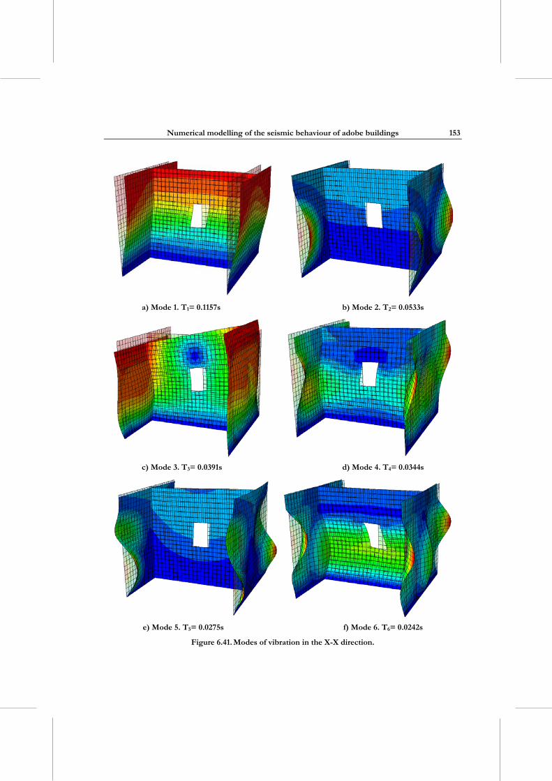
Numerical modelling of the seismic behaviour of adobe buildings
153
a) Mode 1. T1= 0.1157s b) Mode 2. T2= 0.0533s
c) Mode 3. T3= 0.0391s d) Mode 4. T4= 0.0344s
e) Mode 5. T5= 0.0275s f) Mode 6. T6= 0.0242s
Figure 6.41. Modes of vibration in the X-X direction.
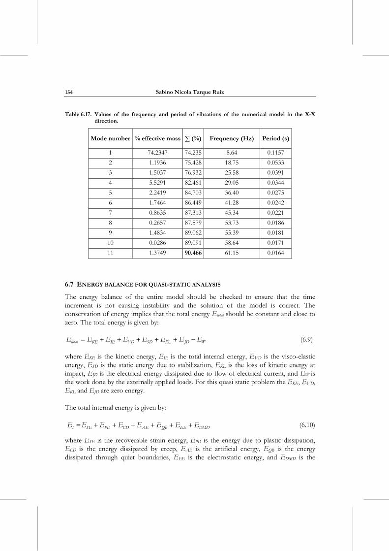
Sabino Nicola Tarque Ruíz
154
Table 6.17. Values of the frequency and period of vibrations of the numerical model in the X-X direction.
Mode number % effective mass ∑ (%) Frequency (Hz) Period (s)
1 74.2347 74.235 8.64 0.1157
2 1.1936 75.428 18.75 0.0533
3 1.5037 76.932 25.58 0.0391
4 5.5291 82.461 29.05 0.0344
5 2.2419 84.703 36.40 0.0275
6 1.7464 86.449 41.28 0.0242
7 0.8635 87.313 45.34 0.0221
8 0.2657 87.579 53.73 0.0186
9 1.4834 89.062 55.39 0.0181
10 0.0286 89.091 58.64 0.0171
11 1.3749 90.466 61.15 0.0164
6.7 ENERGY BALANCE FOR QUASI-STATIC ANALYSIS
The energy balance of the entire model should be checked to ensure that the time increment is not causing instability and the solution of the model is correct. The conservation of energy implies that the total energy Etotal should be constant and close to zero. The total energy is given by:
total KE IE VD SD KL JD WE E E E E E E E (6.9)
where EKE is the kinetic energy, EIE is the total internal energy, EVD is the visco-elastic energy, ESD is the static energy due to stabilization, EKL is the loss of kinetic energy at impact, EJD is the electrical energy dissipated due to flow of electrical current, and EW is the work done by the externally applied loads. For this quasi static problem the EKE, EVD, EKL and EJD are zero energy.
The total internal energy is given by:
I SE PD CD AE QB EE DMDE E E E E E E E (6.10)
where ESE is the recoverable strain energy, EPD is the energy due to plastic dissipation, ECD is the energy dissipated by creep, EAE is the artificial energy, EQB is the energy dissipated through quiet boundaries, EEE is the electrostatic energy, and EDMD is the
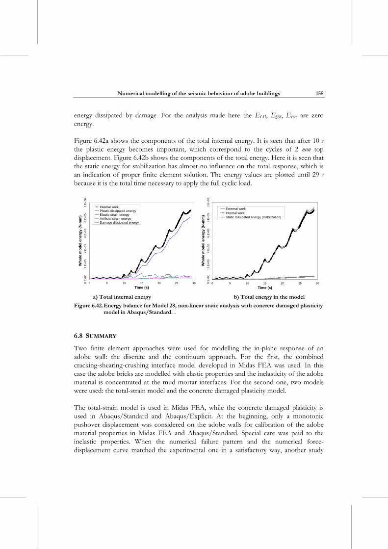
Numerical modelling of the seismic behaviour of adobe buildings
155
energy dissipated by damage. For the analysis made here the ECD, EQB, EEE are zero energy.
Figure 6.42a shows the components of the total internal energy. It is seen that after 10 s the plastic energy becomes important, which correspond to the cycles of 2 mm top displacement. Figure 6.42b shows the components of the total energy. Here it is seen that the static energy for stabilization has almost no influence on the total response, which is an indication of proper finite element solution. The energy values are plotted until 29 s because it is the total time necessary to apply the full cyclic load.
0.E
+00
2.E
+05
4.E
+05
6.E
+05
8.E
+05
1.E
+06
0 5 10 15 20 25 30
Time (s)
Wh
ole
mo
del
en
erg
y (N
-mm
)
Internal workPlastic dissipated energyElastic strain energyArtificial strain energyDamage dissipated energy
0.E
+0
02
.E+
05
4.E
+0
56.
E+
058.
E+
051.
E+
06
0 5 10 15 20 25 30
Time (s)
Wh
ole
mo
del
en
erg
y (N
-mm
)
External workInternal workStatic dissipated energy (stabilization)
a) Total internal energy b) Total energy in the model
Figure 6.42. Energy balance for Model 28, non-linear static analysis with concrete damaged plasticity model in Abaqus/Standard. .
6.8 SUMMARY
Two finite element approaches were used for modelling the in-plane response of an adobe wall: the discrete and the continuum approach. For the first, the combined cracking-shearing-crushing interface model developed in Midas FEA was used. In this case the adobe bricks are modelled with elastic properties and the inelasticity of the adobe material is concentrated at the mud mortar interfaces. For the second one, two models were used: the total-strain model and the concrete damaged plasticity model.
The total-strain model is used in Midas FEA, while the concrete damaged plasticity is used in Abaqus/Standard and Abaqus/Explicit. At the beginning, only a monotonic pushover displacement was considered on the adobe walls for calibration of the adobe material properties in Midas FEA and Abaqus/Standard. Special care was paid to the inelastic properties. When the numerical failure pattern and the numerical force-displacement curve matched the experimental one in a satisfactory way, another study

Sabino Nicola Tarque Ruíz
156
was done in Abaqus/Standard to simulate the cyclic response on an adobe wall. This way, damage factors and stiffness recovery in tension and compression were calibrated in view of the complete seismic analysis of adobe walls (see Chapter 7). The cyclic response was not able to be reproduced in Midas FEA due to difficulties in convergence for reversal loads.
7. NON-LINEAR DYNAMIC ANALYSIS OF AN ADOBE MODULE
In sections 3.5 and 3.6 pseudo-static and dynamic tests carried out on an adobe wall and on an adobe module at the Pontificia Universidad Católica del Perú, respectively, were presented. In chapter 6 the material parameters, both elastic and inelastic, for adobe masonry were calibrated using the results of the pseudo-static test. In this chapter, some finite element models of the experimental adobe module are used to simulate numerically its dynamic behaviour on the shake table. The numerical models are created in Abaqus/Standard and Abaqus/Explicit and using the concrete damaged plasticity model. Each model supposes to be an improvement of the previous one.
7.1 SOLUTION APPROACHES FOR SOLVING DYNAMIC PROBLEMS
There are two solution approaches for solving dynamic problems: implicit, which is used in Abaqus/Standard, and explicit, which is used in Abaqus/Explicit. The first one is an iterative approach for solving the system equilibrium. This may have trouble achieving convergence in dynamic analyses with a highly non-linear material behaviour. The explicit method can solve equations directly without iterations, providing in this case a robust method for large dynamic problems. The following description of each solution approach is summarized from Blind and Östlund [2009].
7.1.1 Governing equations
Newton’s second law of motion states that the group of forces acting on a particle is proportional to the time rate of change of its linear momentum,
ij j i i, f u (7.1)
where ij j, is the Cauchy stress, if is the body load, is the density of the material and
iu is the acceleration at the particle.
The traction boundary conditions ij j i i t, n t and the displacement boundary conditions i i tu D , where in is the surface normal, must be satisfies. Equation (7.1) is the strong (or differential) form of the prolem, in most cases impossible to solve in closed form for unknown displacements.
Sabino Nicola Tarque Ruíz
158
The weak form of Equation (7.1) can be obtained by imposing the principle of virtual work, multiplying the differential equation by an arbitrary vector-valued test function v over the entire volume and integrating. The virtual work rate is given in Equation (7.2), which specifies that the work done by external forces subjected to any virtual velocity field is equal to the rate of work done by equilibrating stresses on the rate of deformation of the same virtual velocity field. Another way for understanding Equation (7.2) is that the total potential of the system must be stationary and it is equal to the sum of the strain energy and the potential energy of external forces.
ext i i ij i j i i i iV V V SW W dV dV dV dSint , 0 u v v f v t v (7.2)
In the finite element approximation, the displacement field over a single element is written as a function of the nodal displacements nu premultiples by the shape functions nN :
nn u N u (7.3)
The test function v should be compatible with all kinematic constraints, so it must have the same spatial variation of the real displacements:
n n v N v (7.4)
The right hand side of Equation (7.2) is written:
n T T T Tn n n nV V V S
dV dV dV dS 0v N N u B N f N t (7.5)
Since the virtual velocity is not zero, the expression in brackets must be equal to zero:
T T T Tn n n nV V V S
dV dV dV dS 0N N u B N f N t (7.6)
Matrix B related strains and displacements. Equation (7.6) is composed of the following terms:
Tn nV
dV M N N (7.7)
T
VdV I B (7.8)
T Tn nV S
dV dS P N f N t (7.9)
Numerical modelling of the seismic behaviour of adobe buildings
159
where M , I and P are the mass matrix and the internal and external force vectors, respectively. Then, Equation (7.6), equation of motion, is thus written as follows and solved for u in time:
Mu I u P (7.10)
The previous equation is solved with direct integration schemes. When solving for quasi-static analysis, the inertia forces are considered insignificant.
Implicit and explicit procedures solve for nodal displacements and use the same element calculations to determine the internal element forces. The biggest difference between the two procedures lies in the manner in which the nodal accelerations are computed. In the implicit procedure a set of dependent linear equations is solved by an iterative procedure; while in the explicit procedure a set of independent equations are solved without need of iteration.
7.1.2 Implicit analysis
An implicit analysis implies the solution of a group of non-linear equations from time t to time t dt based on information of t dt ; it requires an iterative procedure. An introduction to the implicit analysis was done in section 6.1.
Abaqus/Standard uses an automatic increment strategy based on a Newton-Raphson iteration solution and a Hilber et al. [1977] time integration for solving quasi-static and dynamic problems. This time integration operator is implicit, which means that the operator matrix must be inverted and a set of simultaneous nonlinear dynamic equilibrium equations must be solved at each time increment.
The Hilber-Hughes-Taylor operator is a generalization of the Newmark operator with controllable numerical damping. The operator replaces the actual equilibrium Equation (7.10) with a balance of d'Alembert forces at the end of the time step and a weighted average of the static forces at the beginning and end of the time step [Abaqus 6.9 SIMULIA 2009]:
t t t t t t t t t t1 0Mu I P I P L (7.11)
where t dtL is the sum of all Lagrange multiplier forces at each step, as specified in Abaqus/Standard. Velocity and displacement integration follows Newmark approach:
t t t t t tt t1 u u u u (7.12)
Sabino Nicola Tarque Ruíz
160
t t t t t t tt t 2 1
2
u u u u u (7.13)
with 21 1 11 , , 0
4 2 3
Parameter controls the numerical damping, and it is useful for dissipating the high frequency noise that is induced when time step size is changed. 0.05 is suggested to quickly remove high frequencies noise without having significant effect on the lower frequency response.
The implicit procedure has two main disadvantages: the formulation of the stiffness matrix of the structure, which becomes ill-conditioned as the material cracks; and the necessity of small time increments for achieving convergence [Karapitta et al. 2011].
7.1.3 Explicit analysis
It was originally created to analyze high-speed dynamic events and models with fast material degradation (such as quasi-brittle materials), which use to give convergence problems when analyzed with implicit procedures. The explicit method solves the state of a finite element model at time t dt solely based on information at time t ; it implies no iterative procedure and no evaluation of the tangent stiffness matrix, which are advantages with respect to the implicit procedure.
The equations of motions are integrated using the central difference integration rule, which is conditionally stable (this means the necessity of a small time increment). The stability limit for this integration rule is approximatively equal to the time for an elastic wave to cross the smallest element dimension in the model.
Abaqus/Explicit solves dynamic problems per each element node. At the beginning of the increment the algorithm solves the following dynamic equilibrium:
Mu P I u (7.14)
where M is the nodal (diagonal) mass matrix, u are the nodal accelerations, P are the nodal forces and I are the internal element forces.
The accelerations are computed at the start of the increment t as:
tt 1 u M P I u (7.15)
Numerical modelling of the seismic behaviour of adobe buildings
161
Since the explicit procedure always uses a diagonal mass matrix, solving for the accelerations is trivial because there are no simultaneous equations to solve. The acceleration of any node is determined completely by its mass and the net force acting on it, making the nodal calculations very inexpensive. Also, both material and geometric nonlinearities are updated [Rosell 2010].
The velocity is computed at the central instant of the time step using a constant acceleration,
t t t t tt ttt t/2
2 2
2
u u u (7.16)
Similarly to the evaluation of the velocity, the displacement at the new time step is computed assuming a constant velocity over the time interval,
t
tt t t t tt 2
u u u (7.17)
To obtain accurate results, the time increment should be quite small to accept constant accelerations during an increment. However, as it was mentioned, each increment is inexpensive because there are no simultaneous equations to solve.
When the displacements are computed, the element strain increments are computed in each integration point followed by the stress computation. The nodal internal forces t tI are then computed and Equation (7.14) is updated to solve another solution step.
7.1.3.1 Stability
A stability limit determines the size of the time increment. Without damping, the stability limit is given by:
tmax
2
(7.18)
with damping:
t 2
max
21
(7.19)
where max is the maximum eigenvalue and is the fraction of critical damping on the highest frequency mode. Besides, the stability limit can be computed looking at the highest frequency of each element in the model,
Sabino Nicola Tarque Ruíz
162
e
d
Lt
cmin
(7.20)
where eL is the characteristic element length and dc is the dilation wave speed, computed as:
dc2
(7.21)
where and are the Lamè constants and is the material density. For a linear elastic material with Poisson’s ratio of zero, the dilation wave speed is:
d Ec
(7.22)
To maintain efficiency on the analysis, the element size should be kept as regular as possible. The stiffer the material, the higher the wave speed, resulting in a smaller stability limit. The higher the density, the lower the wave speed, resulting in a larger stability limit.
If the model contains only one material type, the initial time increment is directly proportional to the size of the smallest element in the mesh. If the mesh contains uniform size elements but contains multiple material descriptions, the element with the highest wave speed will determine the initial time increment.
In Abaqus/Explicit the estimation of t in Equation (7.20) is only approximate. In general, the automatically stable time increment selected by Abaqus/Explicit is less than the one computed by Equation (7.20) by a factor between 0.707 and 1 in a two-dimensional model and between 0.577 and 1 in a three-dimensional model [Abaqus 6.9 SIMULIA 2009].
7.2 IMPLICIT FINITE ELEMENT ANALYSIS OF THE ADOBE MODULE
A finite element model with considering rectangular shell elements was created in Abaqus/Standard for implicit analyses. In the Abaqus option “element controls”, a finite membrane strain and a default drilling hourglass scaling factors are selected. The in-plane element size of the shell is around 100 x 100 mm to maintain a characteristic length h close to 140 mm, which is computed from the diagonal of the shell area. The shell thickness is 280 mm for the right wall and 250 mm for all the other three adobe walls (Figure 7.1). This is because one wall had stucco in the experimental test. The foundation (reinforced concrete beam), the wooden lintels and the wooden beams, which are part of the roof, are modelled as elastic. The adobe masonry is modelled using the concrete
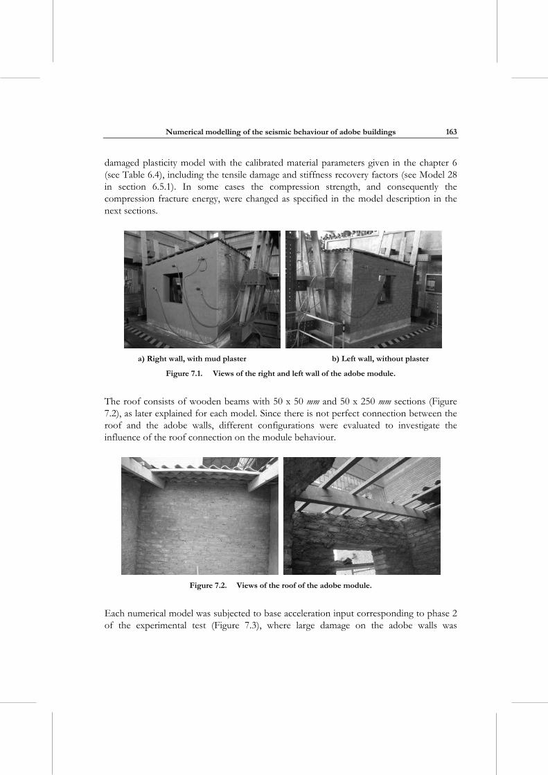
Numerical modelling of the seismic behaviour of adobe buildings
163
damaged plasticity model with the calibrated material parameters given in the chapter 6 (see Table 6.4), including the tensile damage and stiffness recovery factors (see Model 28 in section 6.5.1). In some cases the compression strength, and consequently the compression fracture energy, were changed as specified in the model description in the next sections.
a) Right wall, with mud plaster b) Left wall, without plaster
Figure 7.1. Views of the right and left wall of the adobe module.
The roof consists of wooden beams with 50 x 50 mm and 50 x 250 mm sections (Figure 7.2), as later explained for each model. Since there is not perfect connection between the roof and the adobe walls, different configurations were evaluated to investigate the influence of the roof connection on the module behaviour.
Figure 7.2. Views of the roof of the adobe module.
Each numerical model was subjected to base acceleration input corresponding to phase 2 of the experimental test (Figure 7.3), where large damage on the adobe walls was
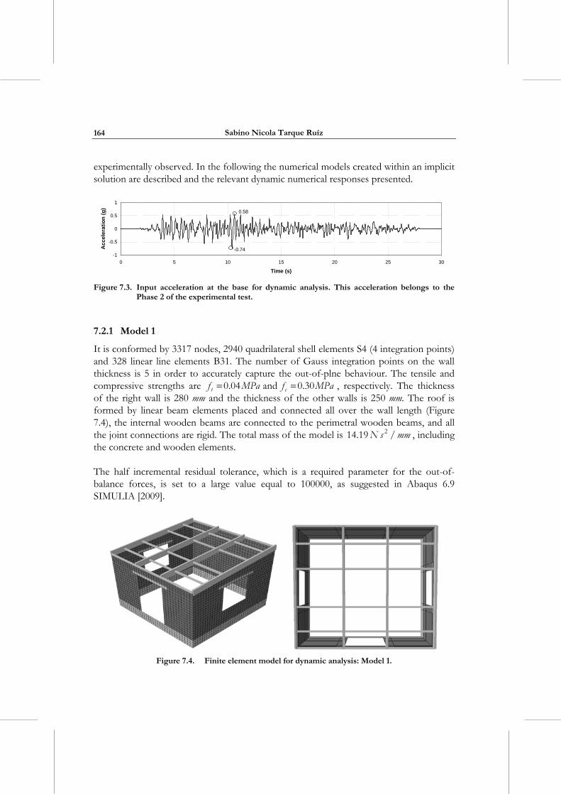
Sabino Nicola Tarque Ruíz
164
experimentally observed. In the following the numerical models created within an implicit solution are described and the relevant dynamic numerical responses presented.
-1
-0.5
0
0.5
1
0 5 10 15 20 25 30
Time (s)
Ac
cele
rati
on
(g
)
-0.74
0.58
Figure 7.3. Input acceleration at the base for dynamic analysis. This acceleration belongs to the
Phase 2 of the experimental test.
7.2.1 Model 1
It is conformed by 3317 nodes, 2940 quadrilateral shell elements S4 (4 integration points) and 328 linear line elements B31. The number of Gauss integration points on the wall thickness is 5 in order to accurately capture the out-of-plne behaviour. The tensile and compressive strengths are tf MPa0.04 and cf MPa0.30 , respectively. The thickness of the right wall is 280 mm and the thickness of the other walls is 250 mm. The roof is formed by linear beam elements placed and connected all over the wall length (Figure 7.4), the internal wooden beams are connected to the perimetral wooden beams, and all the joint connections are rigid. The total mass of the model is N s mm214.19 / , including the concrete and wooden elements.
The half incremental residual tolerance, which is a required parameter for the out-of-balance forces, is set to a large value equal to 100000, as suggested in Abaqus 6.9 SIMULIA [2009].
Figure 7.4. Finite element model for dynamic analysis: Model 1.
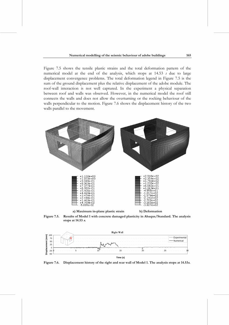
Numerical modelling of the seismic behaviour of adobe buildings
165
Figure 7.5 shows the tensile plastic strains and the total deformation pattern of the numerical model at the end of the analysis, which stops at 14.53 s due to large displacement convergence problems. The total deformation legend in Figure 7.5 is the sum of the ground displacement plus the relative displacement of the adobe module. The roof-wall interaction is not well captured. In the experiment a physical separation between roof and walls was observed. However, in the numerical model the roof still connects the walls and does not allow the overturning or the rocking behaviour of the walls perpendicular to the motion. Figure 7.6 shows the displacement history of the two walls parallel to the movement.
a) Maximum in-plane plastic strain b) Deformation
Figure 7.5. Results of Model 1 with concrete damaged plasticity in Abaqus/Standard. The analysis stops at 14.53 s.
Right Wall
-50
-25
0
25
50
75
100
0 5 10 15 20 25 30
Time (s)
Dis
pla
cem
ent
(mm
)
Experimental
Numerical
Figure 7.6. Displacement history of the right and rear wall of Model 1. The analysis stops at 14.53s.
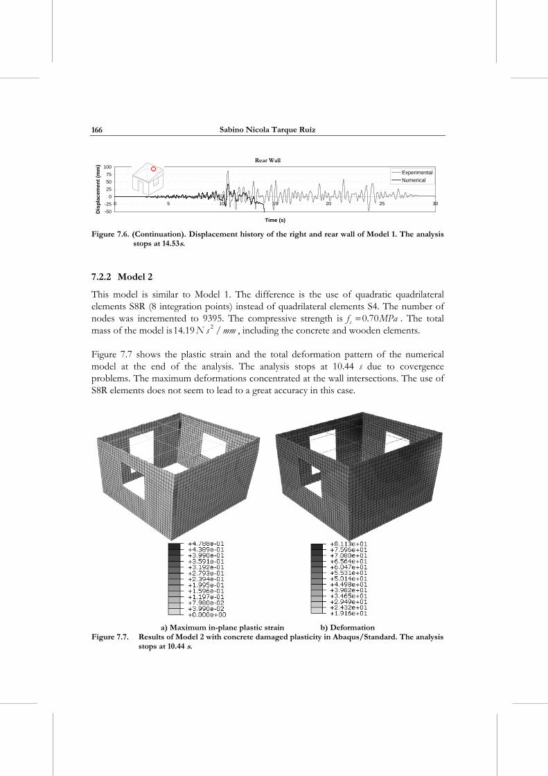
Sabino Nicola Tarque Ruíz
166
Rear Wall
-50
-25
0
25
50
75
100
0 5 10 15 20 25 30
Time (s)
Dis
pla
cem
en
t (m
m)
Experimental
Numerical
Figure 7.6. (Continuation). Displacement history of the right and rear wall of Model 1. The analysis
stops at 14.53s.
7.2.2 Model 2
This model is similar to Model 1. The difference is the use of quadratic quadrilateral elements S8R (8 integration points) instead of quadrilateral elements S4. The number of nodes was incremented to 9395. The compressive strength is cf MPa0.70 . The total mass of the model is N s mm214.19 / , including the concrete and wooden elements.
Figure 7.7 shows the plastic strain and the total deformation pattern of the numerical model at the end of the analysis. The analysis stops at 10.44 s due to covergence problems. The maximum deformations concentrated at the wall intersections. The use of S8R elements does not seem to lead to a great accuracy in this case.
a) Maximum in-plane plastic strain b) Deformation
Figure 7.7. Results of Model 2 with concrete damaged plasticity in Abaqus/Standard. The analysis stops at 10.44 s.
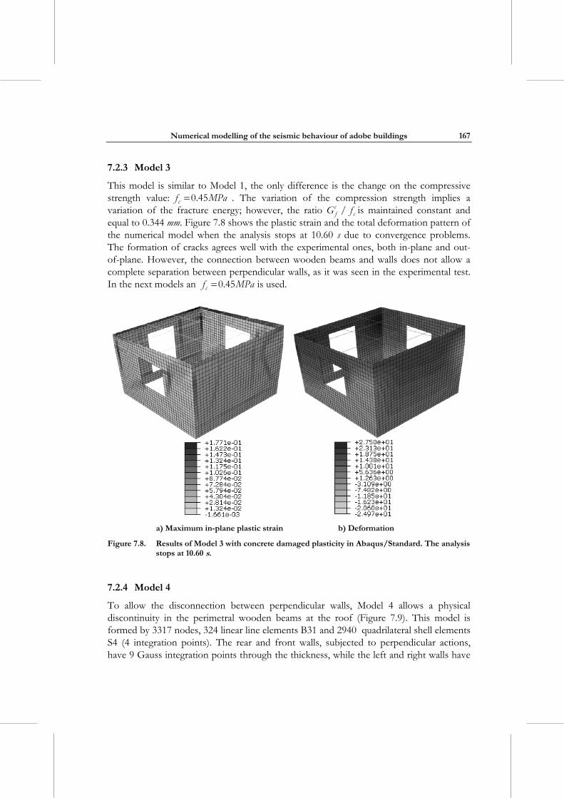
Numerical modelling of the seismic behaviour of adobe buildings
167
7.2.3 Model 3
This model is similar to Model 1, the only difference is the change on the compressive strength value: cf MPa0.45 . The variation of the compression strength implies a variation of the fracture energy; however, the ratio c
f cG f/ is maintained constant and equal to 0.344 mm. Figure 7.8 shows the plastic strain and the total deformation pattern of the numerical model when the analysis stops at 10.60 s due to convergence problems. The formation of cracks agrees well with the experimental ones, both in-plane and out-of-plane. However, the connection between wooden beams and walls does not allow a complete separation between perpendicular walls, as it was seen in the experimental test. In the next models an cf MPa0.45 is used.
a) Maximum in-plane plastic strain b) Deformation
Figure 7.8. Results of Model 3 with concrete damaged plasticity in Abaqus/Standard. The analysis stops at 10.60 s.
7.2.4 Model 4
To allow the disconnection between perpendicular walls, Model 4 allows a physical discontinuity in the perimetral wooden beams at the roof (Figure 7.9). This model is formed by 3317 nodes, 324 linear line elements B31 and 2940 quadrilateral shell elements S4 (4 integration points). The rear and front walls, subjected to perpendicular actions, have 9 Gauss integration points through the thickness, while the left and right walls have
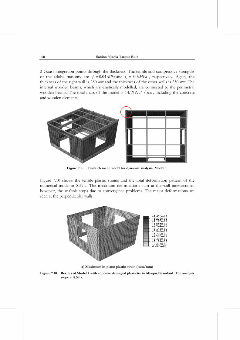
Sabino Nicola Tarque Ruíz
168
3 Gauss integration points through the thickness. The tensile and compressive strengths of the adobe masonry are tf MPa0.04 and cf MPa0.45 , respectively. Again, the thickness of the right wall is 280 mm and the thickness of the other walls is 250 mm. The internal wooden beams, which are elastically modelled, are connected to the perimetral wooden beams. The total mass of the model is N s mm214.19 / , including the concrete and wooden elements.
Figure 7.9. Finite element model for dynamic analysis: Model 1.
Figure 7.10 shows the tensile plastic strains and the total deformation pattern of the numerical model at 8.59 s. The maximum deformations start at the wall intersections; however, the analysis stops due to convergence problems. The major deformations are seen at the perpendicular walls.
a) Maximum in-plane plastic strain (mm/mm)
Figure 7.10. Results of Model 4 with concrete damaged plasticity in Abaqus/Standard. The analysis stops at 8.59 s.
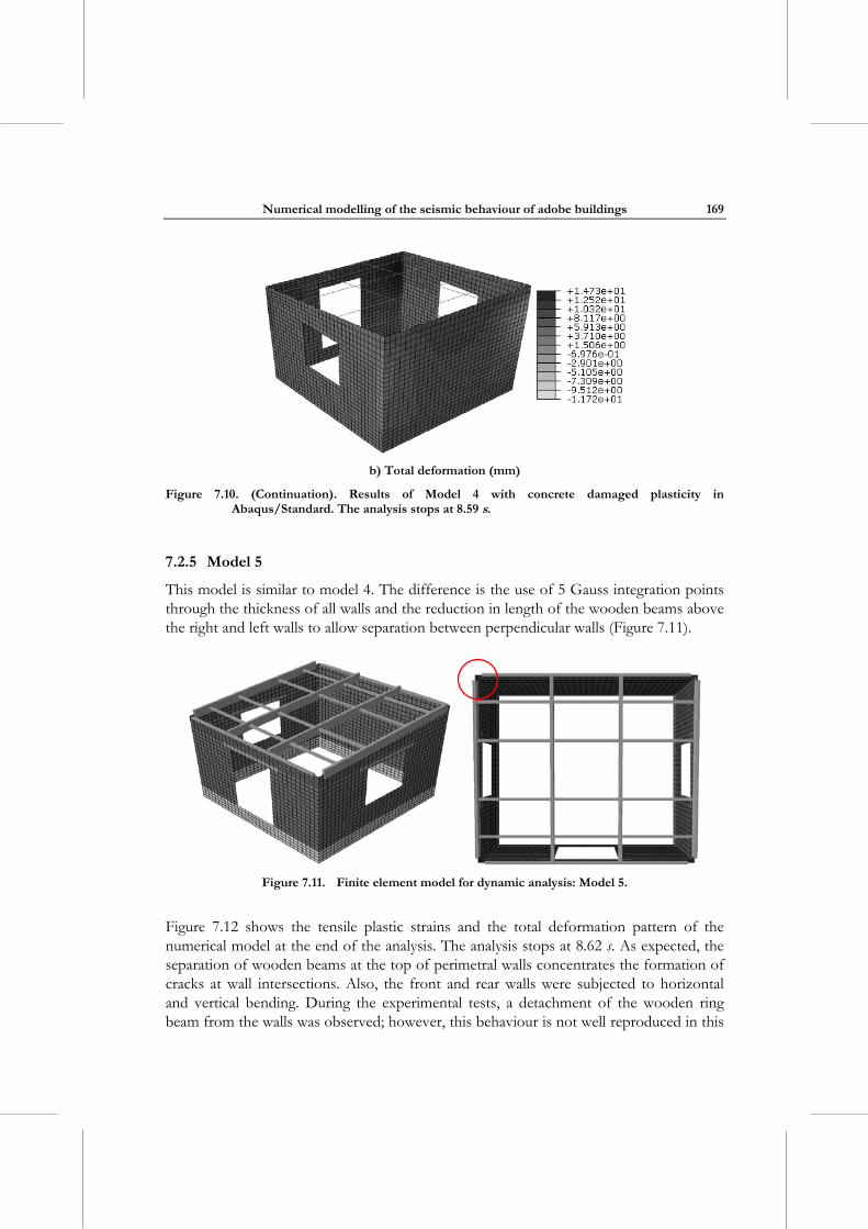
Numerical modelling of the seismic behaviour of adobe buildings
169
b) Total deformation (mm)
Figure 7.10. (Continuation). Results of Model 4 with concrete damaged plasticity in Abaqus/Standard. The analysis stops at 8.59 s.
7.2.5 Model 5
This model is similar to model 4. The difference is the use of 5 Gauss integration points through the thickness of all walls and the reduction in length of the wooden beams above the right and left walls to allow separation between perpendicular walls (Figure 7.11).
Figure 7.11. Finite element model for dynamic analysis: Model 5.
Figure 7.12 shows the tensile plastic strains and the total deformation pattern of the numerical model at the end of the analysis. The analysis stops at 8.62 s. As expected, the separation of wooden beams at the top of perimetral walls concentrates the formation of cracks at wall intersections. Also, the front and rear walls were subjected to horizontal and vertical bending. During the experimental tests, a detachment of the wooden ring beam from the walls was observed; however, this behaviour is not well reproduced in this
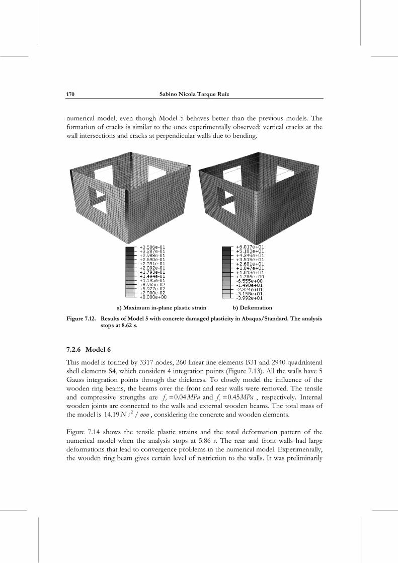
Sabino Nicola Tarque Ruíz
170
numerical model; even though Model 5 behaves better than the previous models. The formation of cracks is similar to the ones experimentally observed: vertical cracks at the wall intersections and cracks at perpendicular walls due to bending.
a) Maximum in-plane plastic strain b) Deformation
Figure 7.12. Results of Model 5 with concrete damaged plasticity in Abaqus/Standard. The analysis stops at 8.62 s.
7.2.6 Model 6
This model is formed by 3317 nodes, 260 linear line elements B31 and 2940 quadrilateral shell elements S4, which considers 4 integration points (Figure 7.13). All the walls have 5 Gauss integration points through the thickness. To closely model the influence of the wooden ring beams, the beams over the front and rear walls were removed. The tensile and compressive strengths are tf MPa0.04 and cf MPa0.45 , respectively. Internal wooden joints are connected to the walls and external wooden beams. The total mass of the model is N s mm214.19 / , considering the concrete and wooden elements.
Figure 7.14 shows the tensile plastic strains and the total deformation pattern of the numerical model when the analysis stops at 5.86 s. The rear and front walls had large deformations that lead to convergence problems in the numerical model. Experimentally, the wooden ring beam gives certain level of restriction to the walls. It was preliminarily
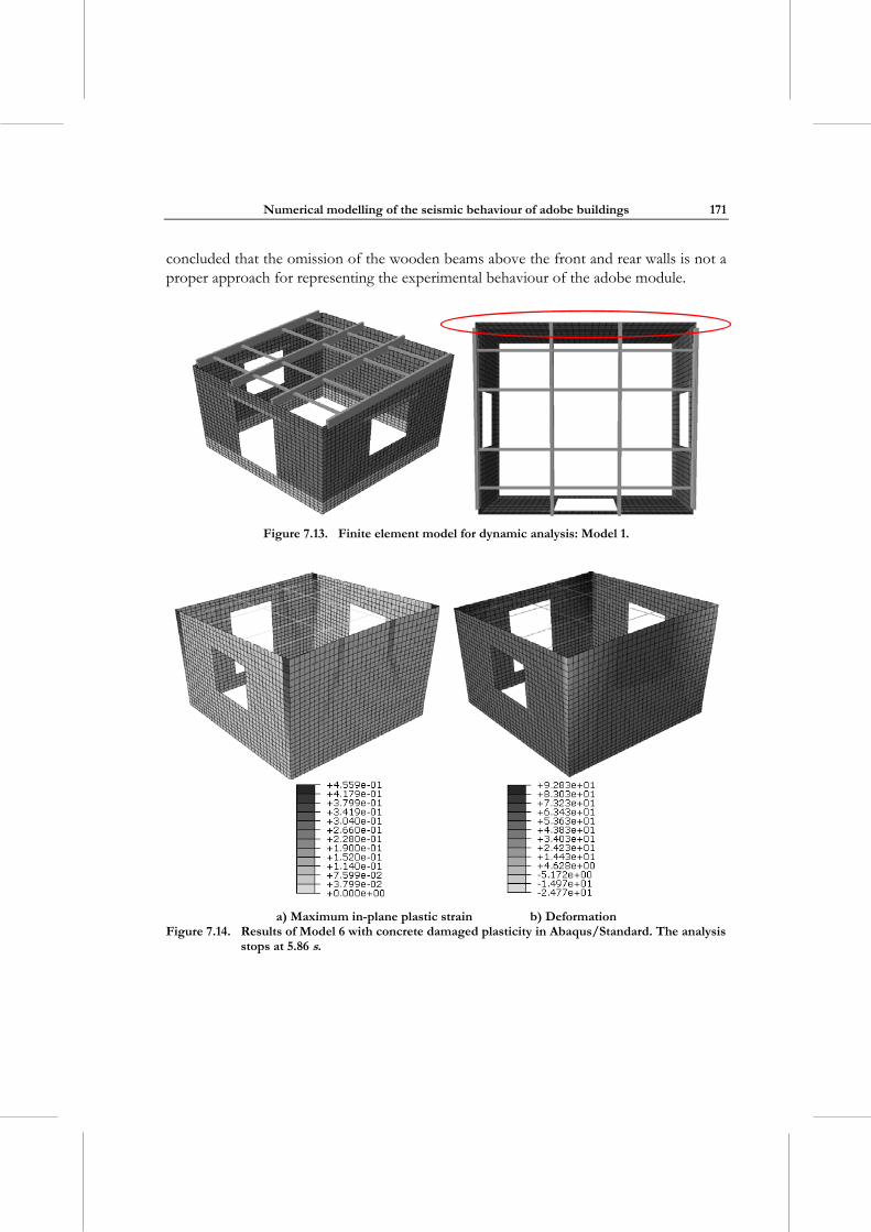
Numerical modelling of the seismic behaviour of adobe buildings
171
concluded that the omission of the wooden beams above the front and rear walls is not a proper approach for representing the experimental behaviour of the adobe module.
Figure 7.13. Finite element model for dynamic analysis: Model 1.
a) Maximum in-plane plastic strain b) Deformation
Figure 7.14. Results of Model 6 with concrete damaged plasticity in Abaqus/Standard. The analysis stops at 5.86 s.
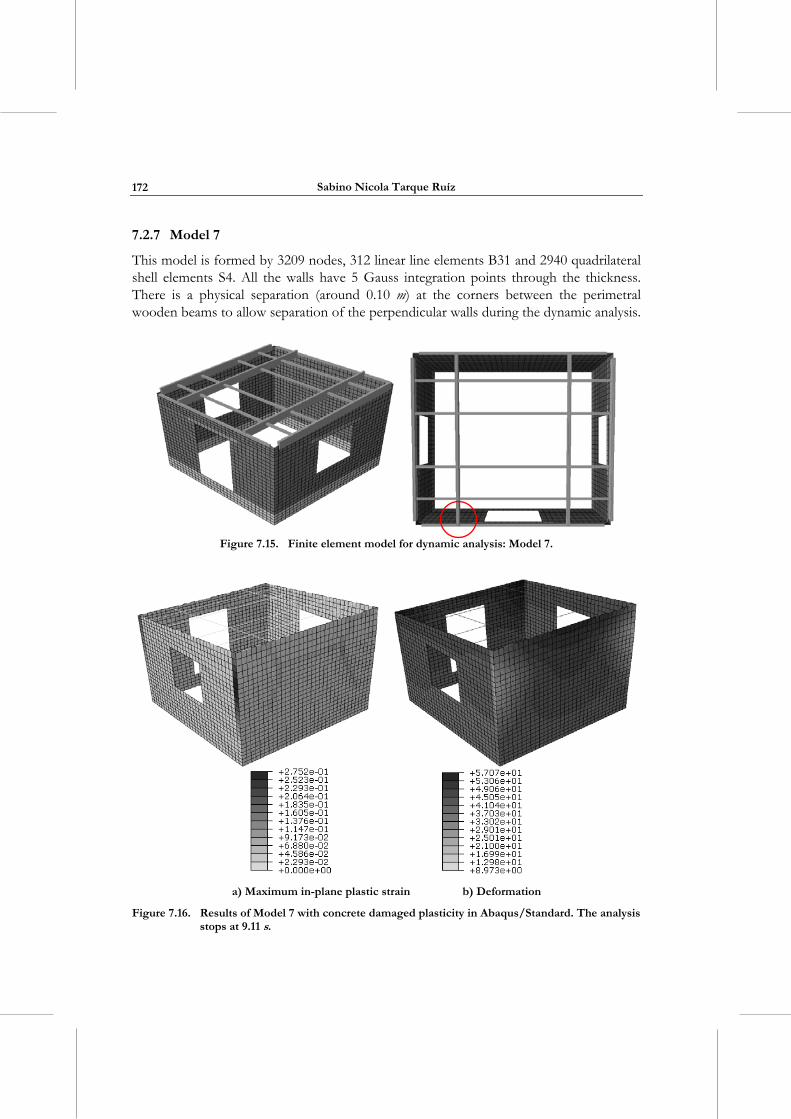
Sabino Nicola Tarque Ruíz
172
7.2.7 Model 7
This model is formed by 3209 nodes, 312 linear line elements B31 and 2940 quadrilateral shell elements S4. All the walls have 5 Gauss integration points through the thickness. There is a physical separation (around 0.10 m) at the corners between the perimetral wooden beams to allow separation of the perpendicular walls during the dynamic analysis.
Figure 7.15. Finite element model for dynamic analysis: Model 7.
a) Maximum in-plane plastic strain b) Deformation
Figure 7.16. Results of Model 7 with concrete damaged plasticity in Abaqus/Standard. The analysis stops at 9.11 s.
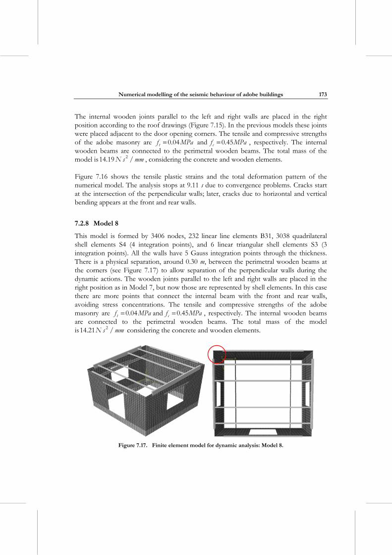
Numerical modelling of the seismic behaviour of adobe buildings
173
The internal wooden joints parallel to the left and right walls are placed in the right position according to the roof drawings (Figure 7.15). In the previous models these joints were placed adjacent to the door opening corners. The tensile and compressive strengths of the adobe masonry are tf MPa0.04 and cf MPa0.45 , respectively. The internal wooden beams are connected to the perimetral wooden beams. The total mass of the model is N s mm214.19 / , considering the concrete and wooden elements.
Figure 7.16 shows the tensile plastic strains and the total deformation pattern of the numerical model. The analysis stops at 9.11 s due to convergence problems. Cracks start at the intersection of the perpendicular walls; later, cracks due to horizontal and vertical bending appears at the front and rear walls.
7.2.8 Model 8
This model is formed by 3406 nodes, 232 linear line elements B31, 3038 quadrilateral shell elements S4 (4 integration points), and 6 linear triangular shell elements S3 (3 integration points). All the walls have 5 Gauss integration points through the thickness. There is a physical separation, around 0.30 m, between the perimetral wooden beams at the corners (see Figure 7.17) to allow separation of the perpendicular walls during the dynamic actions. The wooden joints parallel to the left and right walls are placed in the right position as in Model 7, but now those are represented by shell elements. In this case there are more points that connect the internal beam with the front and rear walls, avoiding stress concentrations. The tensile and compressive strengths of the adobe masonry are tf MPa0.04 and cf MPa0.45 , respectively. The internal wooden beams are connected to the perimetral wooden beams. The total mass of the model is N s mm214.21 / considering the concrete and wooden elements.
Figure 7.17. Finite element model for dynamic analysis: Model 8.
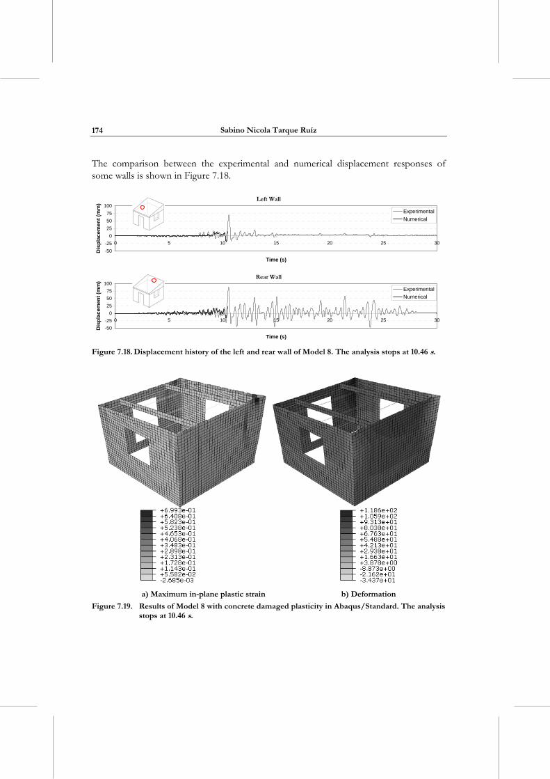
Sabino Nicola Tarque Ruíz
174
The comparison between the experimental and numerical displacement responses of some walls is shown in Figure 7.18.
Left Wall
-50
-25
0
25
50
75
100
0 5 10 15 20 25 30
Time (s)
Dis
pla
cem
ent
(mm
)
Experimental
Numerical
Rear Wall
-50
-25
0
25
50
75
100
0 5 10 15 20 25 30
Time (s)
Dis
pla
cem
ent
(mm
)
Experimental
Numerical
Figure 7.18. Displacement history of the left and rear wall of Model 8. The analysis stops at 10.46 s.
a) Maximum in-plane plastic strain b) Deformation
Figure 7.19. Results of Model 8 with concrete damaged plasticity in Abaqus/Standard. The analysis stops at 10.46 s.
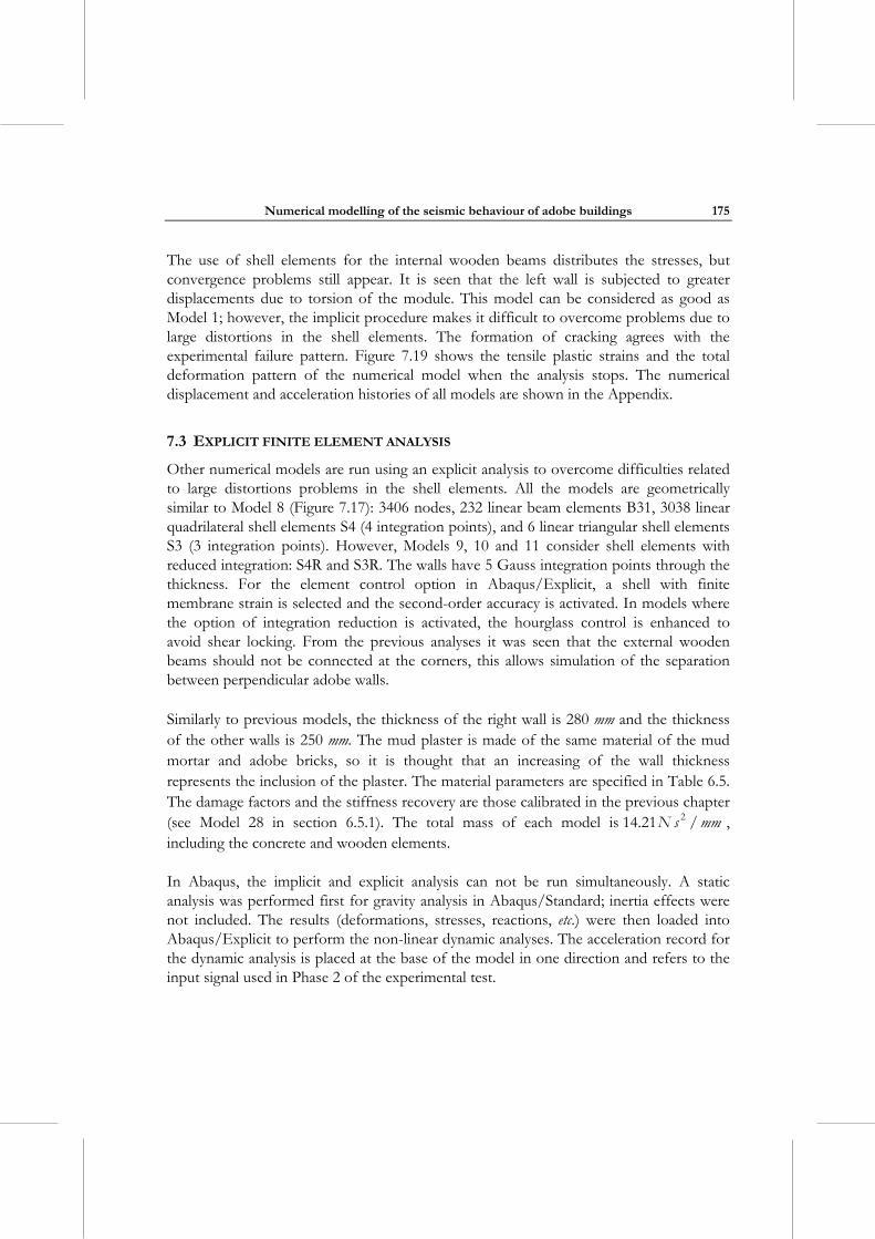
Numerical modelling of the seismic behaviour of adobe buildings
175
The use of shell elements for the internal wooden beams distributes the stresses, but convergence problems still appear. It is seen that the left wall is subjected to greater displacements due to torsion of the module. This model can be considered as good as Model 1; however, the implicit procedure makes it difficult to overcome problems due to large distortions in the shell elements. The formation of cracking agrees with the experimental failure pattern. Figure 7.19 shows the tensile plastic strains and the total deformation pattern of the numerical model when the analysis stops. The numerical displacement and acceleration histories of all models are shown in the Appendix.
7.3 EXPLICIT FINITE ELEMENT ANALYSIS
Other numerical models are run using an explicit analysis to overcome difficulties related to large distortions problems in the shell elements. All the models are geometrically similar to Model 8 (Figure 7.17): 3406 nodes, 232 linear beam elements B31, 3038 linear quadrilateral shell elements S4 (4 integration points), and 6 linear triangular shell elements S3 (3 integration points). However, Models 9, 10 and 11 consider shell elements with reduced integration: S4R and S3R. The walls have 5 Gauss integration points through the thickness. For the element control option in Abaqus/Explicit, a shell with finite membrane strain is selected and the second-order accuracy is activated. In models where the option of integration reduction is activated, the hourglass control is enhanced to avoid shear locking. From the previous analyses it was seen that the external wooden beams should not be connected at the corners, this allows simulation of the separation between perpendicular adobe walls.
Similarly to previous models, the thickness of the right wall is 280 mm and the thickness of the other walls is 250 mm. The mud plaster is made of the same material of the mud mortar and adobe bricks, so it is thought that an increasing of the wall thickness represents the inclusion of the plaster. The material parameters are specified in Table 6.5. The damage factors and the stiffness recovery are those calibrated in the previous chapter (see Model 28 in section 6.5.1). The total mass of each model is N s mm214.21 / , including the concrete and wooden elements.
In Abaqus, the implicit and explicit analysis can not be run simultaneously. A static analysis was performed first for gravity analysis in Abaqus/Standard; inertia effects were not included. The results (deformations, stresses, reactions, etc.) were then loaded into Abaqus/Explicit to perform the non-linear dynamic analyses. The acceleration record for the dynamic analysis is placed at the base of the model in one direction and refers to the input signal used in Phase 2 of the experimental test.
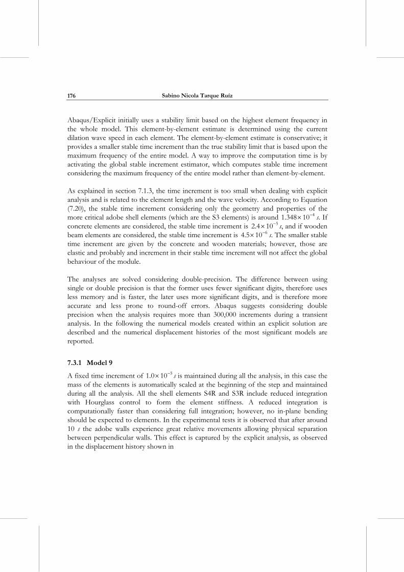
Sabino Nicola Tarque Ruíz
176
Abaqus/Explicit initially uses a stability limit based on the highest element frequency in the whole model. This element-by-element estimate is determined using the current dilation wave speed in each element. The element-by-element estimate is conservative; it provides a smaller stable time increment than the true stability limit that is based upon the maximum frequency of the entire model. A way to improve the computation time is by activating the global stable increment estimator, which computes stable time increment considering the maximum frequency of the entire model rather than element-by-element.
As explained in section 7.1.3, the time increment is too small when dealing with explicit analysis and is related to the element length and the wave velocity. According to Equation (7.20), the stable time increment considering only the geometry and properties of the more critical adobe shell elements (which are the S3 elements) is around 41.348 10 s. If concrete elements are considered, the stable time increment is 52.4 10 s, and if wooden beam elements are considered, the stable time increment is 64.5 10 s. The smaller stable time increment are given by the concrete and wooden materials; however, those are elastic and probably and increment in their stable time increment will not affect the global behaviour of the module.
The analyses are solved considering double-precision. The difference between using single or double precision is that the former uses fewer significant digits, therefore uses less memory and is faster, the later uses more significant digits, and is therefore more accurate and less prone to round-off errors. Abaqus suggests considering double precision when the analysis requires more than 300,000 increments during a transient analysis. In the following the numerical models created within an explicit solution are described and the numerical displacement histories of the most significant models are reported.
7.3.1 Model 9
A fixed time increment of 51.0 10 s is maintained during all the analysis, in this case the mass of the elements is automatically scaled at the beginning of the step and maintained during all the analysis. All the shell elements S4R and S3R include reduced integration with Hourglass control to form the element stiffness. A reduced integration is computationally faster than considering full integration; however, no in-plane bending should be expected to elements. In the experimental tests it is observed that after around 10 s the adobe walls experience great relative movements allowing physical separation between perpendicular walls. This effect is captured by the explicit analysis, as observed in the displacement history shown in
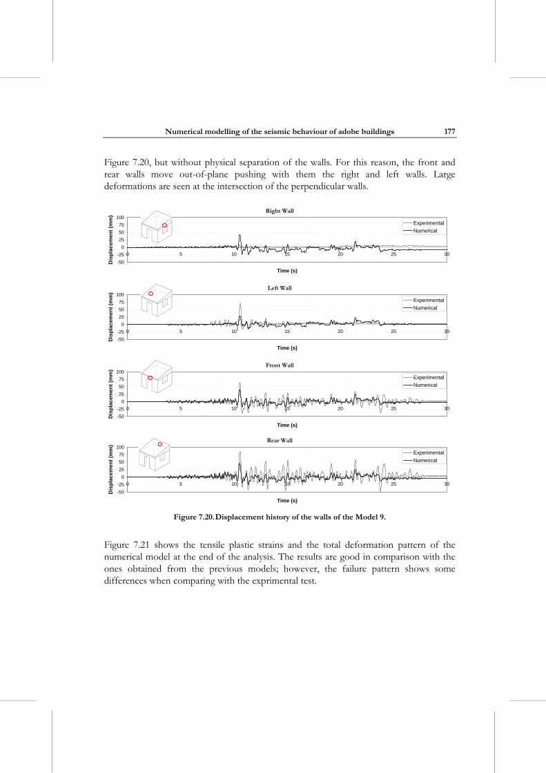
Numerical modelling of the seismic behaviour of adobe buildings
177
Figure 7.20, but without physical separation of the walls. For this reason, the front and rear walls move out-of-plane pushing with them the right and left walls. Large deformations are seen at the intersection of the perpendicular walls.
Right Wall
-50
-25
0
25
50
75
100
0 5 10 15 20 25 30
Time (s)
Dis
pla
cem
ent
(mm
)
Experimental
Numerical
Left Wall
-50
-25
0
25
50
75
100
0 5 10 15 20 25 30
Time (s)
Dis
pla
cem
ent
(mm
)
Experimental
Numerical
Front Wall
-50
-25
0
25
50
75
100
0 5 10 15 20 25 30
Time (s)
Dis
pla
cem
ent
(mm
)
Experimental
Numerical
Rear Wall
-50
-25
0
25
50
75
100
0 5 10 15 20 25 30
Time (s)
Dis
pla
cem
ent
(mm
)
Experimental
Numerical
Figure 7.20. Displacement history of the walls of the Model 9.
Figure 7.21 shows the tensile plastic strains and the total deformation pattern of the numerical model at the end of the analysis. The results are good in comparison with the ones obtained from the previous models; however, the failure pattern shows some differences when comparing with the exprimental test.
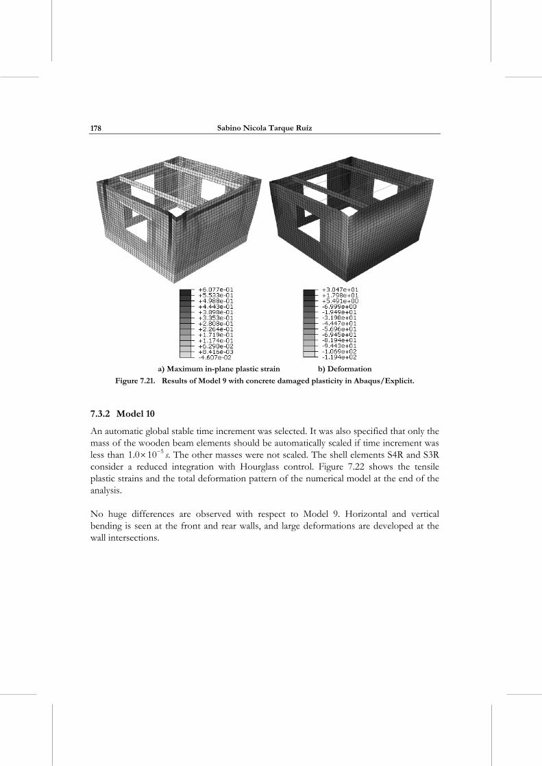
Sabino Nicola Tarque Ruíz
178
a) Maximum in-plane plastic strain b) Deformation
Figure 7.21. Results of Model 9 with concrete damaged plasticity in Abaqus/Explicit.
7.3.2 Model 10
An automatic global stable time increment was selected. It was also specified that only the mass of the wooden beam elements should be automatically scaled if time increment was less than 51.0 10 s. The other masses were not scaled. The shell elements S4R and S3R consider a reduced integration with Hourglass control. Figure 7.22 shows the tensile plastic strains and the total deformation pattern of the numerical model at the end of the analysis.
No huge differences are observed with respect to Model 9. Horizontal and vertical bending is seen at the front and rear walls, and large deformations are developed at the wall intersections.
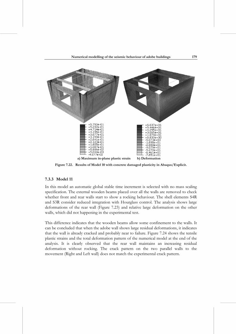
Numerical modelling of the seismic behaviour of adobe buildings
179
a) Maximum in-plane plastic strain b) Deformation
Figure 7.22. Results of Model 10 with concrete damaged plasticity in Abaqus/Explicit.
7.3.3 Model 11
In this model an automatic global stable time increment is selected with no mass scaling specification. The external wooden beams placed over all the walls are removed to check whether front and rear walls start to show a rocking behaviour. The shell elements S4R and S3R consider reduced integration with Hourglass control. The analysis shows large deformations of the rear wall (Figure 7.23) and relative large deformation on the other walls, which did not happening in the experimental test.
This difference indicates that the wooden beams allow some confinement to the walls. It can be concluded that when the adobe wall shows large residual deformations, it indicates that the wall is already cracked and probably near to failure. Figure 7.24 shows the tensile plastic strains and the total deformation pattern of the numerical model at the end of the analysis. It is clearly observed that the rear wall maintains an increasing residual deformation without rocking. The crack pattern on the two parallel walls to the movement (Right and Left wall) does not match the experimental crack pattern.

Sabino Nicola Tarque Ruíz
180
Front Wall
-50
-25
0
25
50
75
100
0 5 10 15 20 25 30
Dis
pla
cem
ent
(mm
)
Experimental
Numerical
Rear Wall
-50
-25
0
25
50
75
100
0 5 10 15 20 25 30
Time (s)
Dis
pla
ce
me
nt
(mm
)
Experimental
Numerical
Figure 7.23. Displacement history of the walls of the Model 11.
a) Maximum in-plane plastic strain b) Deformation
Figure 7.24. Results of Model 11 with concrete damaged plasticity in Abaqus/Explicit.
7.3.4 Model 12
In this model the wooden beams are placed again all over the wall lengths but are not connected at the corners (see Figure 7.17). An automatic global stable time increment is selected with specification of scaling the wooden mass if the time increment is less than
51.0 10 s. In contrast to the previous models run in Abaqus/Explicit, this model has shell elements with full integration S4 to capture better the out-of-plane actions on the
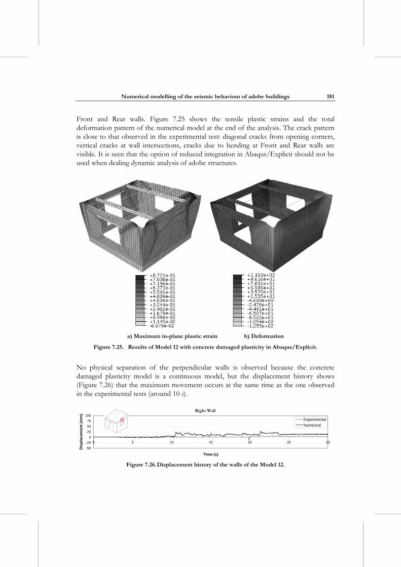
Numerical modelling of the seismic behaviour of adobe buildings
181
Front and Rear walls. Figure 7.25 shows the tensile plastic strains and the total deformation pattern of the numerical model at the end of the analysis. The crack pattern is close to that observed in the experimental test: diagonal cracks from opening corners, vertical cracks at wall intersections, cracks due to bending at Front and Rear walls are visible. It is seen that the option of reduced integration in Abaqus/Explicti should not be used when dealing dynamic analysis of adobe structures.
a) Maximum in-plane plastic strain b) Deformation
Figure 7.25. Results of Model 12 with concrete damaged plasticity in Abaqus/Explicit.
No physical separation of the perpendicular walls is observed because the concrete damaged plasticity model is a continuous model, but the displacement history shows (Figure 7.26) that the maximum movement occurs at the same time as the one observed in the experimental tests (around 10 s).
Right Wall
-50
-25
0
25
50
75
100
0 5 10 15 20 25 30
Time (s)
Dis
pla
cem
ent
(mm
)
Experimental
Numerical
Figure 7.26. Displacement history of the walls of the Model 12.
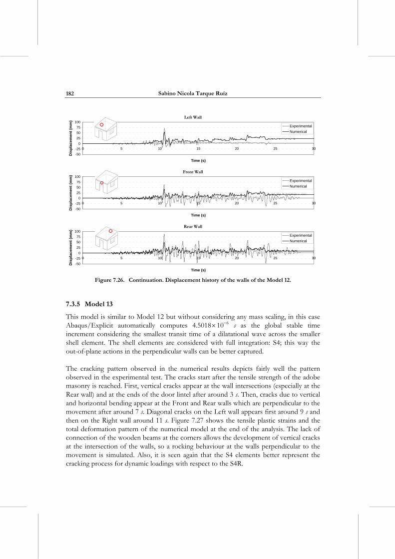
Sabino Nicola Tarque Ruíz
182
Left Wall
-50
-25
0
25
50
75
100
0 5 10 15 20 25 30
Time (s)
Dis
pla
cem
ent
(mm
)
Experimental
Numerical
Front Wall
-50
-25
0
25
50
75
100
0 5 10 15 20 25 30
Time (s)
Dis
pla
cem
ent
(mm
)
Experimental
Numerical
Rear Wall
-50
-25
0
25
50
75
100
0 5 10 15 20 25 30
Time (s)
Dis
pla
cem
ent
(mm
)
Experimental
Numerical
Figure 7.26. Continuation. Displacement history of the walls of the Model 12.
7.3.5 Model 13
This model is similar to Model 12 but without considering any mass scaling, in this case Abaqus/Explicit automatically computes 64.5018 10 s as the global stable time increment considering the smallest transit time of a dilatational wave across the smaller shell element. The shell elements are considered with full integration: S4; this way the out-of-plane actions in the perpendicular walls can be better captured.
The cracking pattern observed in the numerical results depicts fairly well the pattern observed in the experimental test. The cracks start after the tensile strength of the adobe masonry is reached. First, vertical cracks appear at the wall intersections (especially at the Rear wall) and at the ends of the door lintel after around 3 s. Then, cracks due to vertical and horizontal bending appear at the Front and Rear walls which are perpendicular to the movement after around 7 s. Diagonal cracks on the Left wall appears first around 9 s and then on the Right wall around 11 s. Figure 7.27 shows the tensile plastic strains and the total deformation pattern of the numerical model at the end of the analysis. The lack of connection of the wooden beams at the corners allows the development of vertical cracks at the intersection of the walls, so a rocking behaviour at the walls perpendicular to the movement is simulated. Also, it is seen again that the S4 elements better represent the cracking process for dynamic loadings with respect to the S4R.
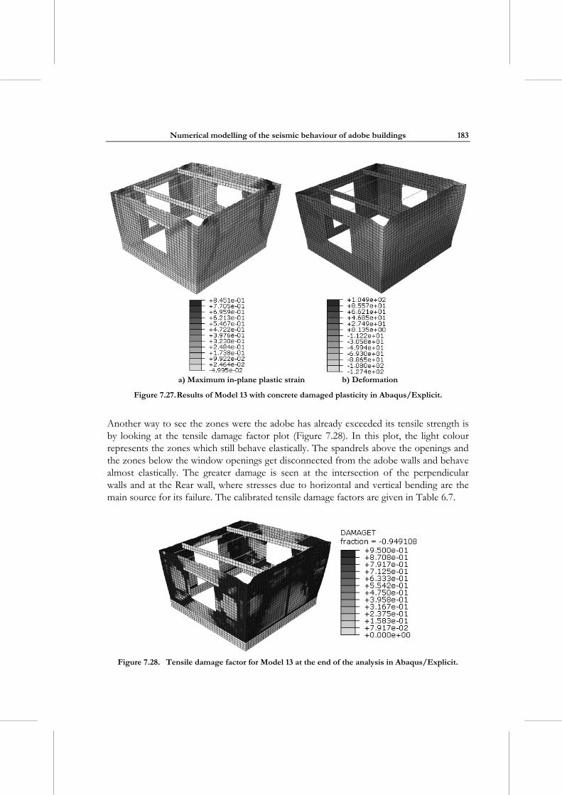
Numerical modelling of the seismic behaviour of adobe buildings
183
a) Maximum in-plane plastic strain b) Deformation
Figure 7.27. Results of Model 13 with concrete damaged plasticity in Abaqus/Explicit.
Another way to see the zones were the adobe has already exceeded its tensile strength is by looking at the tensile damage factor plot (Figure 7.28). In this plot, the light colour represents the zones which still behave elastically. The spandrels above the openings and the zones below the window openings get disconnected from the adobe walls and behave almost elastically. The greater damage is seen at the intersection of the perpendicular walls and at the Rear wall, where stresses due to horizontal and vertical bending are the main source for its failure. The calibrated tensile damage factors are given in Table 6.7.
Figure 7.28. Tensile damage factor for Model 13 at the end of the analysis in Abaqus/Explicit.
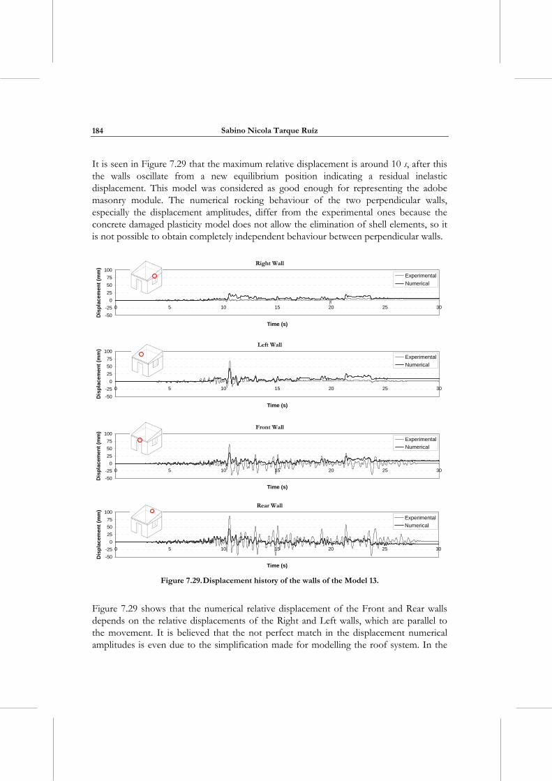
Sabino Nicola Tarque Ruíz
184
It is seen in Figure 7.29 that the maximum relative displacement is around 10 s, after this the walls oscillate from a new equilibrium position indicating a residual inelastic displacement. This model was considered as good enough for representing the adobe masonry module. The numerical rocking behaviour of the two perpendicular walls, especially the displacement amplitudes, differ from the experimental ones because the concrete damaged plasticity model does not allow the elimination of shell elements, so it is not possible to obtain completely independent behaviour between perpendicular walls.
Right Wall
-50
-25
0
25
50
75
100
0 5 10 15 20 25 30
Time (s)
Dis
pla
cem
ent
(mm
)
Experimental
Numerical
Left Wall
-50
-25
0
25
50
75
100
0 5 10 15 20 25 30
Time (s)
Dis
pla
cem
ent
(mm
)
Experimental
Numerical
Front Wall
-50
-25
0
25
50
75
100
0 5 10 15 20 25 30
Time (s)
Dis
pla
cem
ent
(mm
)
Experimental
Numerical
Rear Wall
-50
-25
0
25
50
75
100
0 5 10 15 20 25 30
Time (s)
Dis
pla
cem
ent
(mm
)
Experimental
Numerical
Figure 7.29. Displacement history of the walls of the Model 13.
Figure 7.29 shows that the numerical relative displacement of the Front and Rear walls depends on the relative displacements of the Right and Left walls, which are parallel to the movement. It is believed that the not perfect match in the displacement numerical amplitudes is even due to the simplification made for modelling the roof system. In the
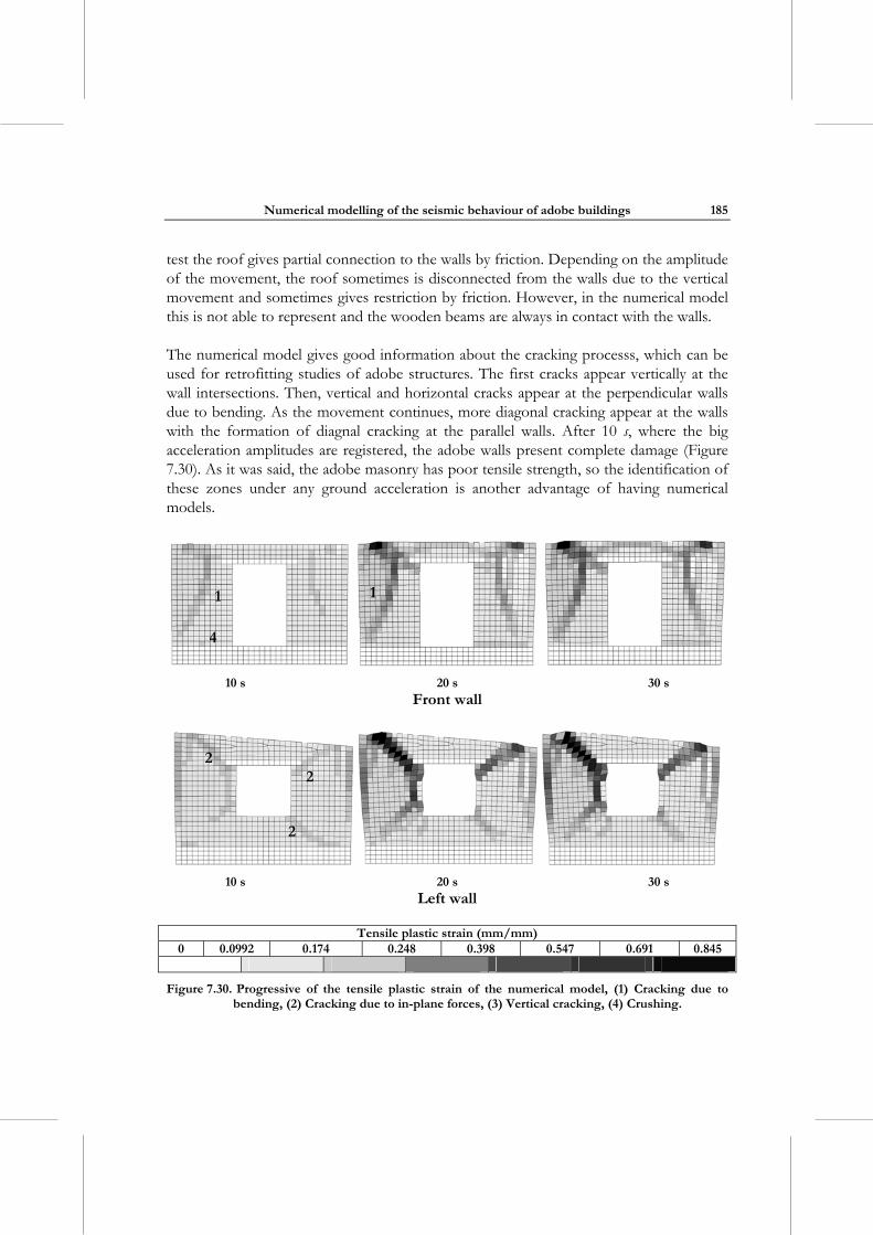
Numerical modelling of the seismic behaviour of adobe buildings
185
test the roof gives partial connection to the walls by friction. Depending on the amplitude of the movement, the roof sometimes is disconnected from the walls due to the vertical movement and sometimes gives restriction by friction. However, in the numerical model this is not able to represent and the wooden beams are always in contact with the walls.
The numerical model gives good information about the cracking processs, which can be used for retrofitting studies of adobe structures. The first cracks appear vertically at the wall intersections. Then, vertical and horizontal cracks appear at the perpendicular walls due to bending. As the movement continues, more diagonal cracking appear at the walls with the formation of diagnal cracking at the parallel walls. After 10 s, where the big acceleration amplitudes are registered, the adobe walls present complete damage (Figure 7.30). As it was said, the adobe masonry has poor tensile strength, so the identification of these zones under any ground acceleration is another advantage of having numerical models.
10 s 20 s 30 s
Front wall
10 s 20 s 30 s
Left wall
Tensile plastic strain (mm/mm) 0 0.0992 0.174 0.248 0.398 0.547 0.691 0.845
Figure 7.30. Progressive of the tensile plastic strain of the numerical model, (1) Cracking due to bending, (2) Cracking due to in-plane forces, (3) Vertical cracking, (4) Crushing.
1 1
2 2
2
4
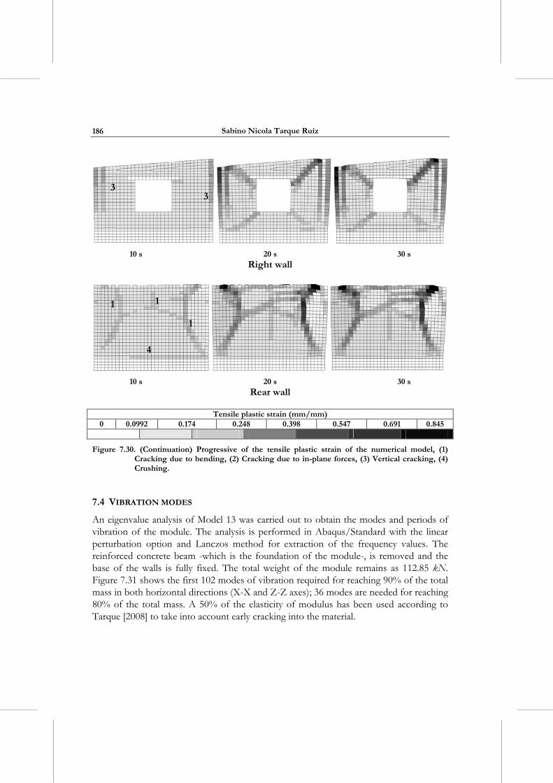
Sabino Nicola Tarque Ruíz
186
10 s 20 s 30 s
Right wall
10 s 20 s 30 s
Rear wall
Tensile plastic strain (mm/mm) 0 0.0992 0.174 0.248 0.398 0.547 0.691 0.845
Figure 7.30. (Continuation) Progressive of the tensile plastic strain of the numerical model, (1) Cracking due to bending, (2) Cracking due to in-plane forces, (3) Vertical cracking, (4) Crushing.
7.4 VIBRATION MODES
An eigenvalue analysis of Model 13 was carried out to obtain the modes and periods of vibration of the module. The analysis is performed in Abaqus/Standard with the linear perturbation option and Lanczos method for extraction of the frequency values. The reinforced concrete beam -which is the foundation of the module-, is removed and the base of the walls is fully fixed. The total weight of the module remains as 112.85 kN. Figure 7.31 shows the first 102 modes of vibration required for reaching 90% of the total mass in both horizontal directions (X-X and Z-Z axes); 36 modes are needed for reaching 80% of the total mass. A 50% of the elasticity of modulus has been used according to Tarque [2008] to take into account early cracking into the material.
3 3
1
1
4
1
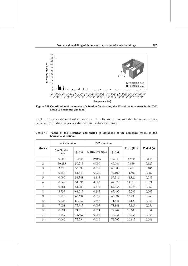
Numerical modelling of the seismic behaviour of adobe buildings
187
0
5
10
15
20
25
30
35
40
45
50
55
6.97
0
11.8
26
16.7
30
18.9
53
25.0
21
28.4
60
31.6
81
33.7
97
37.3
72
39.4
62
42.7
02
43.9
66
47.5
27
50.9
58
53.5
50
55.5
38
58.4
30
60.3
94
63.8
04
65.5
88
66.6
85
67.4
71
69.0
31
71.7
36
74.3
18
76.4
43
Frequency (Hz)
Eff
ec
tiv
e m
ass
(%)
Horizontal X-XHorizontal Z-Z
Figure 7.31. Contribution of the modes of vibration for reaching the 90% of the total mass in the X-X
and Z-Z horizontal direction.
Table 7.1 shows detailed information on the effective mass and the frequency values obtained from the analysis for the first 26 modes of vibration.
Table 7.1. Values of the frequency and period of vibrations of the numerical model in the horizontal direction.
X-X direction Z-Z direction
Mode# % effective
mass ∑ (%) % effective mass ∑ (%)
Freq. (Hz) Period (s)
1 0.000 0.000 49.046 49.046 6.970 0.143
2 50.215 50.215 0.000 49.046 7.859 0.127
3 3.675 53.890 0.037 49.083 9.427 0.106
4 0.458 54.348 0.020 49.102 11.502 0.087
5 0.000 54.348 8.413 57.516 11.826 0.085
6 0.047 54.396 4.563 62.079 14.010 0.071
7 0.584 54.980 5.275 67.354 14.973 0.067
8 9.737 64.717 0.143 67.497 15.289 0.065
9 1.916 66.634 0.597 68.094 16.730 0.060
10 0.225 66.859 3.747 71.841 17.122 0.058
11 7.058 73.917 0.007 71.848 17.829 0.056
12 0.094 74.010 0.894 72.742 18.603 0.054
13 1.459 75.469 0.008 72.751 18.953 0.053
14 0.066 75.534 0.016 72.767 20.817 0.048
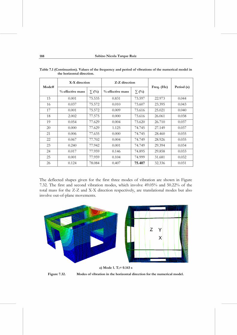
Sabino Nicola Tarque Ruíz
188
Table 7.1 (Continuation). Values of the frequency and period of vibrations of the numerical model in the horizontal direction.
X-X direction Z-Z direction Mode#
% effective mass ∑ (%) % effective mass ∑ (%) Freq. (Hz) Period (s)
15 0.001 75.535 0.831 73.597 22.973 0.044
16 0.037 75.572 0.010 73.607 23.395 0.043
17 0.001 75.572 0.009 73.616 25.021 0.040
18 2.002 77.575 0.000 73.616 26.061 0.038
19 0.054 77.629 0.004 73.620 26.710 0.037
20 0.000 77.629 1.125 74.745 27.149 0.037
21 0.006 77.635 0.000 74.745 28.460 0.035
22 0.067 77.702 0.004 74.749 28.926 0.035
23 0.240 77.942 0.001 74.749 29.394 0.034
24 0.017 77.959 0.146 74.895 29.858 0.033
25 0.001 77.959 0.104 74.999 31.681 0.032
26 0.124 78.084 0.407 75.407 32.336 0.031
The deflected shapes given for the first three modes of vibration are shown in Figure 7.32. The first and second vibration modes, which involve 49.05% and 50.22% of the total mass for the Z-Z and X-X direction respectively, are translational modes but also involve out-of-plane movements.
a) Mode 1. T1= 0.143 s
Figure 7.32. Modes of vibration in the horizontal direction for the numerical model.
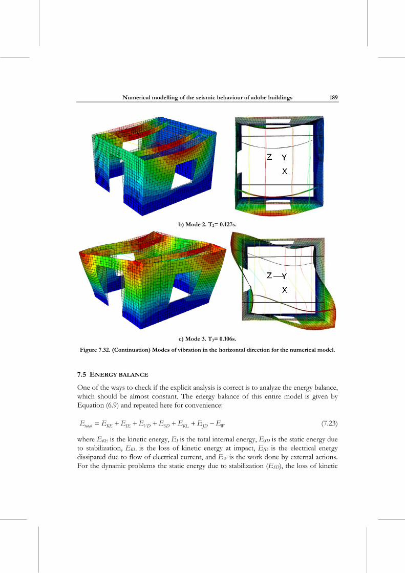
Numerical modelling of the seismic behaviour of adobe buildings
189
b) Mode 2. T2= 0.127s.
c) Mode 3. T3= 0.106s.
Figure 7.32. (Continuation) Modes of vibration in the horizontal direction for the numerical model.
7.5 ENERGY BALANCE
One of the ways to check if the explicit analysis is correct is to analyze the energy balance, which should be almost constant. The energy balance of this entire model is given by Equation (6.9) and repeated here for convenience:
total KE IE VD SD KL JD WE E E E E E E E (7.23)
where EKE is the kinetic energy, EI is the total internal energy, ESD is the static energy due to stabilization, EKL is the loss of kinetic energy at impact, EJD is the electrical energy dissipated due to flow of electrical current, and EW is the work done by external actions. For the dynamic problems the static energy due to stabilization (ESD), the loss of kinetic
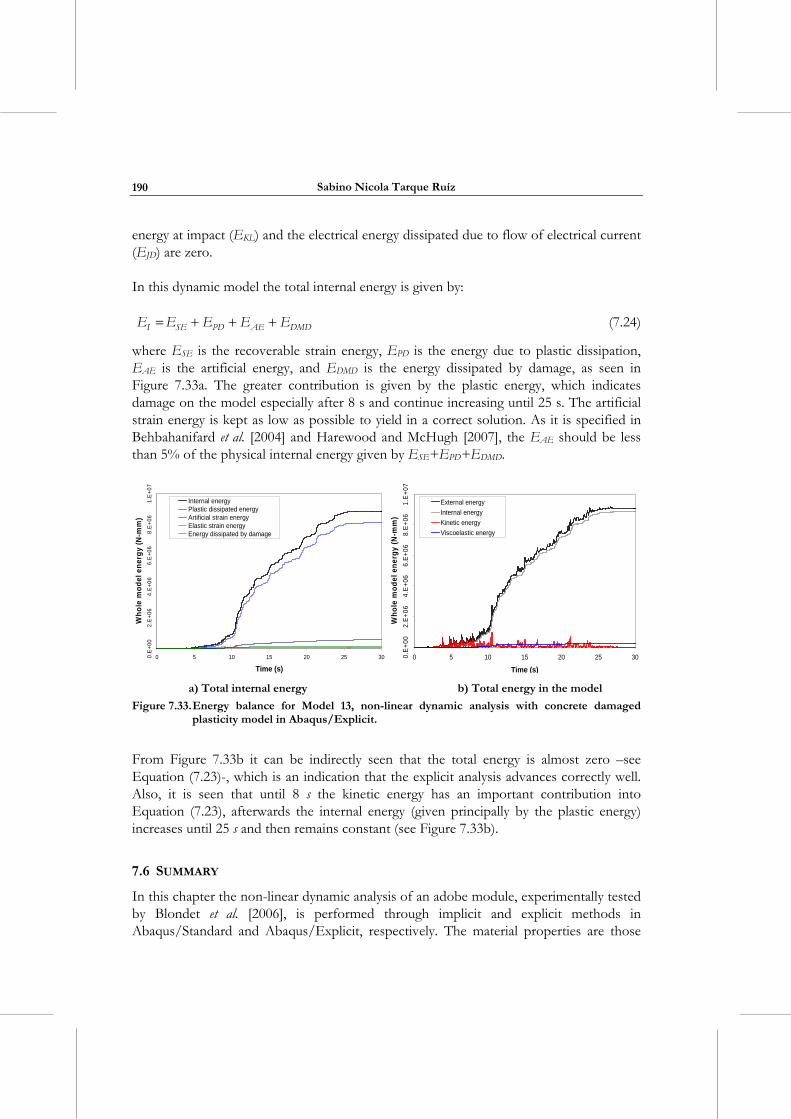
Sabino Nicola Tarque Ruíz
190
energy at impact (EKL) and the electrical energy dissipated due to flow of electrical current (EJD) are zero.
In this dynamic model the total internal energy is given by:
I SE PD AE DMDE E E E E (7.24)
where ESE is the recoverable strain energy, EPD is the energy due to plastic dissipation, EAE is the artificial energy, and EDMD is the energy dissipated by damage, as seen in Figure 7.33a. The greater contribution is given by the plastic energy, which indicates damage on the model especially after 8 s and continue increasing until 25 s. The artificial strain energy is kept as low as possible to yield in a correct solution. As it is specified in Behbahanifard et al. [2004] and Harewood and McHugh [2007], the EAE should be less than 5% of the physical internal energy given by ESE+EPD+EDMD.
0.E
+0
02
.E+
064.
E+
06
6.E
+06
8.E
+06
1.E
+0
7
0 5 10 15 20 25 30
Time (s)
Wh
ole
mo
del
en
erg
y (N
-mm
)
Internal energyPlastic dissipated energyArtificial strain energyElastic strain energyEnergy dissipated by damage
0.E
+00
2.E
+0
64
.E+
066
.E+
06
8.E
+0
61
.E+
07
0 5 10 15 20 25 30
Time (s)
Wh
ole
mo
del
en
erg
y (N
-mm
)
External energy
Internal energy
Kinetic energy
Viscoelastic energy
a) Total internal energy b) Total energy in the model
Figure 7.33. Energy balance for Model 13, non-linear dynamic analysis with concrete damaged plasticity model in Abaqus/Explicit.
From Figure 7.33b it can be indirectly seen that the total energy is almost zero –see Equation (7.23)-, which is an indication that the explicit analysis advances correctly well. Also, it is seen that until 8 s the kinetic energy has an important contribution into Equation (7.23), afterwards the internal energy (given principally by the plastic energy) increases until 25 s and then remains constant (see Figure 7.33b).
7.6 SUMMARY
In this chapter the non-linear dynamic analysis of an adobe module, experimentally tested by Blondet et al. [2006], is performed through implicit and explicit methods in Abaqus/Standard and Abaqus/Explicit, respectively. The material properties are those
Numerical modelling of the seismic behaviour of adobe buildings
191
calibrated in the previous chapter making use of the results from an experimental cyclic test carried out on an adobe wall.
The dynamic experimental adobe module was unidirectionally subjected to three levels of displacement records at the base for reproducing the seismic behaviour of adobe structures. A separation of the perpendicular walls was observed due to vertical cracks. The crack pattern of the parallel walls followed a diagonal direction, while the walls perpendicular to the movement had cracks due to horizontal and vertical bending.
The numerical model is subjected to an acceleration record at the base related to phase 2 of the experimental test, which had a maximum base displacement of 80 mm. The numerical results are compared with the experimental crack pattern and the displacement records measured in all the walls. To simulate the poor connection between the top wooden beams and the adobe walls, the wooden beam elements were reduced in length to avoid a physical connection at the corners (see Figure 7.17).
The numerical models were built with shell elements for representing the adobe masonry. The models run with an implicit method had convergence problems due to large element distortions. The total time of the input signal was 30 s, the analysis stopped around 10 s. However, this restriction was not seen with the models run with an explicit method. The advantages and disadvantages of the two methods are illustrated in this chapter.
From all the numerical models the best approach was Model 13, which considers quadrilateral shell elements S4 without integration reduction. The time increment for the analysis is selected automatically by Abaqus/Explicit without considering mass scaling for increasing the time increment. The assumption of no connection between the wooden beams at the corner improves the numerical results. Besides, the energy balance analysis shows that the numerical model behaves well. Therefore, it is concluded that the calibrated adobe material properties are suitable for using into non-linear dynamic analysis of other adobe structure configurations.

8. SUMMARY AND CONCLUSIONS
This thesis deals with the analysis of adobe masonry with emphasis on the selection of its elastic and inelastic parameters. The gathered experimental data derives basically from static and dynamic tests carried out at the Pontificia Universidad Católica del Perú. The numerical results of an adobe wall and an adobe module, run in Midas FEA and Abaqus, show a strong agreement with the experimental results in terms of failure pattern and seismic capacity.
Peru, as many other countries, has a strong tradition in adobe construction. However, the good tradition is being lost; for example, new adobe houses located along the Peruvian coastline do not follow an acceptable geometrical configuration such as thicker walls with buttresses and small openings at the walls. The necessity of building with thinner walls is related to the small land size relatively available for low incomes families, which almost in all cases build without taking into account any seismic reinforcement or improvement. Therefore, the seismic vulnerability of adobe houses increases due to the lack of good construction practices.
The seismic behaviour of unreinforced adobe constructions seems to follow a common failure sequence: the roof is not rigid enough to guarantee a rigid diaphragm so the adobe walls behave independently and are very vulnerable to out of plane loads. During the earthquakes the walls separates from each other due to the large vertical cracks that appear at the wall intersections. Simultaneously, diagonal cracks start at the wall openings and cracks due to horizontal and vertical bending break the walls into small rigid blocks, followed by wall overturning if the movement continues. The roof collapses after the walls fall down. One way to reduce the high seismic risk is by understanding how adobe structures (considering different configurations and different uses, e.g. houses, churches, monuments) behave under different levels of ground motion. Considering the high cost of the experimental tests, the numerical modelling of adobe constructions is an option for understanding its seismic behaviour.
Little work has been published on modelling of adobe structures. It appears that the best approach is to use finite element models developed for other britlle materials, mainly concrete and masonry. Two general approaches were seen here: the micro-modelling and the macro-modelling. The first one related with the discontinuous or discrete approach and the second one with the continuum approach. The principal input for these
Sabino Nicola Tarque Ruíz
194
approaches are the constitutive laws in tension, compression and shear in the elastic and inelastic range. Information on mechanical properties is however scarce for adobe masonry. Micro-modelling is used for analysis of small masonry structures and especially for understanding the behaviour of the brick-mortar interface; while macro-modelling is used for representing large structures with distributed damage. Another approach for modelling masonry structures is by an equivalent frame method; which can be considered within a macro-modelling approach.
In this thesis the material parameters of adobe masonry are calibrated for the two finite element approaches previously mentioned and implemented into Midas FEA and Abaqus (standard and explicit). For the micro-modelling the composite model developed by Lourenço [1996] for fired brick masonry is used in Midas FEA. This model allows concentrating all the inelasticity (tension, compression and shear) at the mortar joints. Following this approach the adobe wall tested under cyclic loads by Blondet et al. [2005] is reproduced here in Midas FEA but considering only monotonic displacements. The numerical results match quiet well the failure pattern and seismic capacity of the experimental test until certain displacement level, but the analysis stops due to convergence problems. Although the material parameters seems to be correctly calibrated (see Table 6.3), it is recommended to elaborate a test campaign to obtain experimentally the constitutive laws for tension and shear at the mud mortar joints and compression tests of the composite (brick plus mortar). Since adobe is a brittle material, displacement controlled tests can be a good option for capturing the inelastic range. The author recommends using the data specified in Table 6.3 within a discrete approach.
For the macro-modelling two finite element models are used: the total-strain model implemented in Midas FEA and the concrete damaged plasticity model implemented in Abaqus (within a standard and explicit solution). Unlike fired clay masonry, the adobe masonry can be considered as a homogeneous and isotropic material due to the similarity in material properties between the adobe bricks and the mud mortar joints. Generally, the adobe bricks are fabricated and after some time they are used for construction, in this case the mud mortar has not the same age of the bricks and the dry process between mortar and bricks can generate weak zones at the bed and head contact zones.
Similarly to the work done with the discrete approach, the material properties of the adobe masonry in the macro-models are calibrated based on the cyclic test of an adobe wall. Special attention is paid to simulate the crack opening/closing due to tension. Again, the failure pattern and the seismic capacity is quiet well represented and it is concluded that the calibrated material parameters shown in Table 6.4 (for Midas FEA, total-strain model) and Table 6.5 (for Abaqus, concrete damaged plasticity model) can be used for analysis of other geometrical configurations of adobe structures. The adobe module dynamically tested by Blondet et al. [2006] was reproduced using Abaqus/Implicit
Numerical modelling of the seismic behaviour of adobe buildings
195
and Abaqus/Explicit. The acceleration record related to the displacement input used in the experimental tests was applied at the base of the numerical module. The results match well the displacement and acceleration responses measured at the adobe walls (see Appendix). However, the solution within an implicit approach has problems of convergence due to the formation of cracking in the walls, while the analysis with explicit solution does not have convergence problems.
An explicit analysis (Abaqus/Explicit) is adequate for dealing with dynamic problems with quasi-brittle material and contact problems. The integration scheme allows continuing computing the displacement field at the shell elements avoiding convergence problems due to progressive degradation and progressive loss of the material integrity.
The continuum models do not allow the physical separation of the rigid blocks produced by the movement, for this reason the rocking behaviour of the adobe walls are not perfectly captured by the model run in Abaqus, but it is still good enough to understand the cracking process and to identify the zones where the adobe masonry behaves inelastically. According to the non-linear dynamic analysis of the adobe module the numerical displacement response of the walls shows some dependency between the parallel and perpendicular walls; however, in the experimental model a physical separation (vertical cracks) was observed at the union of the walls allowing a rocking behaviour at the walls perpendicular to the movement and a quasi rigid movement at the parallel walls. When high relative displacements are read in the displacement history of the walls, the failure pattern should be controlled to check if vertical cracks are produced at the wall intersection zones.
According to section 6.2.1 it is shown that the governing material property in the adobe masonry is the tension strength and the tensile softening. Here a ft= 0.04 MPa with I
fG = 0.01 N/mm and h≈ 140 mm is recommended for further analyses. The compression behaviour of the adobe masonry does not affect the seismic capacity of the walls. However, a lower bound of the compression strength fc = 0.30 MPa could be considered, with a ratio of c
f cG f/ = 0.344 mm. Analyses with fc= 0.7 MPa were also carried out and the results did not vary too much. Here it is recommended to use fc= 0.45 MPa maintaining the ratio c
f cG f/ = 0.344 mm. The elastic behaviour of the adobe masonry is greatly controlled by the elasticity modulus E, which is considered between 200 to 230 MPa. Lower values of E seem to underestimate the seismic capacity of the masonry. If the analysis requires a given shear retention factor, a value of 0.05 is suggested. Besides, a small dilatancy angle is considered, similarly to masonry structures [Lourenço 1996]. The material parameters shown in Table 6.5 are specified for numerical analysis of adobe structures with different configurations within an explicit solution.
Sabino Nicola Tarque Ruíz
196
Because of the importance of the roof on the seismic behavior of the adobe module, sSpecial attention was placed in understanding the interaction between the roof (formed by wooden beams) and the walls. Experimentally, the wooden beams were attached to the adobe walls through steel nails and mud mortar. During the first phase of the test (with maximum total displacement at the base of 30 mm) separation between the wooden beams and the walls were observed, especially at the wall corners. During the phase 2, which was analyzed in this work, this detachment is clearly seen at the walls perpendicular to the movement, causing the rocking behavior. The effect of partial connection between the wooden beams and the walls has been studied in the finite element models. The best solution was to simulate detachment of the wooden beams from the walls by removing some linear wooden elements close to the wall intersections. When dealing with the analysis of other structures, special attention should be placed to the roof simulation and to evaluate the possibilities of allowing vertical cracking at the wall intersections if they do not have any confining element.
The general conclusion of this thesis is the acceptability of micro and macro modelling for the analysis of adobe structures; besides, the author recommends to use the second approach (continuum model) since the adobe material is reasonable well modelled as a homogeneous material and its behaviour can be represented by a calibrated tension and compression behaviour. The calibrated material parameters for new analyses are given in Table 6.5. It is also recommended to follow when possible an explicit method. In this case the concrete damaged plasticity model should be used.
Although the results achieved in this research, further detailed work should be addressed, namely to:
characterize the mechanical behaviour of adobe material. In this case, an exhaustive experimental campaign should be developed to investigate the linear and the non-linear material properties of the adobe masonry. Since adobe is a brittle material, the testing setups to be adopted should capture the post maximum strength response, thus displacement controlled tests are suggested.
study the influence of roof-wall connections in the response of the constructions. It was seen that the roof system conformed by wooden beams are normally not properly connected to the adobe walls. Those are just attached with steel nails which were disconnected from the walls during the dynamic test. In the research developed in this thesis a simplification of the connection was assumed in the numerical models, reducing the wooden beam length and disconnecting them from the walls at the corners. However, simplified non-linear response of this interaction mechanism should be proposed and calibrated with experimental results.
Numerical modelling of the seismic behaviour of adobe buildings
197
study other type of adobe structures. The macro-modelling approach suggested in this research work can be extended to the analysis of other adobe structures with different configurations, especially for the evaluation of the seismic vulnerability of historic structures as houses, churches and convents, frequently found in Latin-American countries. With this, the weak zones of adobe structures can be identified and based on these results retrofitting solutions may be proposed.
study retrofitting solutions for adobe constructions. The efficiency of different strengthening solutions (invasive and non-invasive) can be numerically assessed, estimating the benefits in terms of post-elastic behaviour of the retrofitted adobe structures, namely ductility and energy dissipation capacity.

REFERENCES
Abaqus 6.9 SIMULIA. [2009] “Abaqus/CAE Extended Funcionality EF2,” Manual, Dassault Systemss Corporation, Providence, RI, USA.
Ali, S. S., and Page, A. W. [1987] “Finite Element Model for Masonry Subjected to Concentrated Loads,” Journal of Structural Engineering, Vol. 114, No.8, p. 1761.
Amadei, B., Sture, S., Saeb, S., and Atkinson, R. H. [1989] “An evaluation of masonry joint shear strength in existing buildings,” Report, Dept. Civ., Envir., and Arch. Engrg., University of Colorado, Boulder, Colorado, USA.
Arya, S. K., and Hegemier, G. A. [1978] “On nonlinear response prediction of concrete masonry assemblies,” Proceedings of North American Masonry Conference, Boulder, Colorado, USA, pp. 19.1-19.24.
Attard, M. M., Nappi, A., and Tin-Loi, F. [2007] “Modeling Fracture in Masonry,” Journal of Structural Engineering, Vol. 133, No.10, p. 1385.
Attard, M. M., and Tin-Loi, F. [1999] “Fracture simulation using a discrete triangular element,” Proceedings of Mechanics of Structures and Materials, M. Bradford and R. Q. Bridge, eds., A. A. Balkema, Sydney, Australia.
Attard, M. M., and Tin-Loi, F. [2005] “Numerical simulation of quasibrittle fracture in concrete,” Engineering Fracture Mechanics, Vol. 72, No.3, pp. 387-411.
Bažant, Zdeněk P., and Oh, B. H. [1983] “Crack band theory for fracture of concrete,” Matériaux et Constructions, Vol. 16, No.3, pp. 155-177.
Behbahanifard, M. R., Grondin, G. Y., and Elwi, A. E. [2004] “Analysis of steel plate shear walls using explicti finite element method,” Proceedings of 13th World Conference on Earthquake Engineering, Vancouver, Canada.
Blind, N., and Östlund, R. [2009] “Analysis of an engine frame subjected to large imbalance loads,” Master Thesis, Luleá University of Technology, Porsön, Sweden.
Sabino Nicola Tarque Ruíz
200
Blondet, M., Ginocchio, F., Marsh, C., Ottazzi, G., Villa-García, G., and Yep, J. [1988] “Shaking table test of improved adobe masonry houses,” Proceedings of 9th World Conference on Earthquake Engineering, Tokyo-Kyoto, Japan.
Blondet, M., Madueño, I., Torrealva, D., Villa-García, G., and Ginocchio, F. [2005] “Using industrial materials for the construction of safe adobe houses in seismic areas,” Proceedings of Earth Build 2005 Conference, Sydney, Australia.
Blondet, M., Torrealva, D., Vargas, J., Tarque, N., and Velásquez, J. [2006] “Seismic reinforcement of adobe houses,” Proceedings of 1st European Conference on Earthquake Engineering and Seismology, Geneva, Switzerland.
Blondet, M., Vargas, J., Velásquez, J., and Tarque, N. [2006] “Experimental Study of Synthetic Mesh Reinforcement of Historical Adobe Buildings,” Proceedings of Structural Analysis of Historical Constructions, P. B. Lourenço, P. Roca, C. Modena, and Agrawal. S., eds., New Delhi, India, pp. 1-8.
Blondet, M., Vargas, J., Villa-García, G., Torrealva, D., and Tarque Ruíz, N. [2005] “Refuerzo de construcciones de adobe con elementos producidos industrialmente: Ensayos de simulación sísmica,” Report, Division of Civil Enginering, Pontificia Universidad Católica del Perú, Lima, Peru.
Blondet, M., Vargas, J., and Tarque, N. [2008a] “Observed behaviour of earthen structures during the Pisco earthquake (Peru),” Proceedings of 14th World Conference on Earthquake Engineering, Beijing, China.
Blondet, M., Vargas, J., and Tarque, N. [2008b] “Avaılable low-cost technologıes to ımprove the seısmıc performance of earthen houses ın seısmıc areas,” Proceedings of Kerpic08 - Learning from earthquake architecture in climate change., Lefkosa, Northen Cyprus.
Blondet, M., Vargas, J., and Villa-García, G. [2008] “Reparación de grietas en construcciones históricas de tierra en áreas sísmicas. Parte IV: aplicación y desarrollo de nuevos métodos de inyección,” Report, Division of Civil Engineering, Pontifcia Universidad Católica del Perú, Lima, Peru.
Blondet, M., Villa-García, G., and Brzev, S. [2003] “Earthquake-Resistant Construction of Adobe Buildings: A Tutorial,” (M. Greene, ed.), Report, EERI/IAEE World Housing Enciclopedy, Okland, California, USA.
Blondet, M., and Vargas, J. [1978] “Investigación sobre vivienda rural,” Report, Division of Civil Engineering, Pontificia Universidad Católica del Perú, Lima, Peru.
Numerical modelling of the seismic behaviour of adobe buildings
201
de Borst, René. [1991] “Computational methods in non-linear solid mechanics. Part 2: physical non-linearity,” Report, Delft University of Technology, Delft, The Netherlands.
de Borst, René, and Nauta, P. [1985] “Non-orthogonal cracks in a smeared finite element model,” Report, Delft University of Technology, Delft, The Netherlands.
Brignola, A., Frumento, S., Lagomarsino, Sergio, and Podestà, S. [2008] “Identification of Shear Parameters of Masonry Panels Through the In-Situ Diagonal Compression Test,” International Journal of Architectural Heritage, Vol. 3, No.1, pp. 52-73.
CENAPRED. [2003] Reinforcement methods for self-construction of rural housing (in Spanish), Mexico City, Mexico.
CTAR/COPASA, GTZ, PUCP, and SENCICO. [2002] Terremoto? ¡Mi casa sí resiste! – Manual de construcción para viviendas sismo resistentes en adobe, Lima, Peru.
CUR. [1997] Structural masonry: a experimental/numerical basis for practical design rules (in Dutch), (J. G. Rots, ed.), A. A. Balkema/Rotterdam/Brookfield, Gouda, The Netherlands.
Calderini, C., Cattari, S., and Lagomarsino, S. [2009] “In plane seismic response of unreifnorced masonry walls: comparison between detailed and equivalent frame models,” ECCOMAS Thematic Conference on Computational Methods in Structural Dynamics and Earthquake Engineering, M. Papadrakakis, N. D. Lagaros, and M. Fragiadakis, eds., Rhodes, Greece.
Cao, Z., and Watanabe, H. [2004] “Earthquake response predication and retroftiing techniques of adobe structures,” Proceedings of 13th World Conference on Earthquake Engineering, Vancouver, Canada.
Chen, W.-F., and Han, D.-J. [1988] Plasticity for structural engineers, Springer-Verlag, New York, USA, p. 606.
Cope, R. J., Rao, P. V., Clark, L. A., and Norris, P. [1980] “Modelling of reinforced concrete behaviour for finite element analysis of bridge slabs,” International Conference: Numerical methods for non-linear problems, Pineridge Press, Swansea, Wales, United Kindom, pp. 457-470.
Cruz, J. S., Barros, J., and Azevedo, Á. [2004] “Elasto-plastic multi-fixed smeared crack model for concrete,” Report 04-DEC/E-05, University of Minho, Minho, Portugal.
Cundall, P. A. [1971] “A computer model for simulating progressive large scale movements in blocky rock systems,” Proceedings of Symposium on Rock Fracture (ISRM), Nancy, France.
Sabino Nicola Tarque Ruíz
202
Van Der Pluijm, R. [1993] “Shear behaviour of bed joints,” Proceedings of 6th North American Masonry Conference, A. A. Hamid and H. G. Harris, eds., Drexel University, Philadelphia, Pennsylvania, USA, pp. 125-136.
Dowling, D. [2004] “Adobe housing in El Salvador: Earthquake performance and seismic improvement,” Geological Society of America Special Papers, I. Rose, J. J. Bommer, D. L. López, M. J. Carr, and J. J. Major, eds., pp. 281-300.
Easton, D. [2007] The Rammed Earth House, (J. Barstow, ed.), Chelsea Publishing Company, Vertmon, USA, p. 266.
Elsaigh, W. A. M. H. [2007] “Modelling the behaviour of steel fibre reinforced concrete pavements,” Ph.D. Thesis, University of Petroria, Petroria, South Africa.
Feenstra, P. H. [1993] “Computational aspects of biaxial stress in plain and reinforced concrete,” Ph. D. Thesis, Delft University of Technology, Delft, The Netherlands.
Feenstra, P. H., and de Borst, Rene. [1992] “The use of various crack models in F.E. analysis of reinforced concrete panels,” Proceedings of First International Conference on Fracture Mechanics of Concrete Structures: FraMCoS1, Zdenek P. Bažant, ed., Taylor and Francis, Breckenridge, Colorado, USA.
Feenstra, P. H., and Rots, J. G. [2001] “Comparison of Concrete Models for Cyclic Loading,” Modelling of Inelastic Behaviour of RC Structures under Seismis Loads, P. Benson Shing and T.-aki Tanabe, eds., American Society of Civil Engineers, USA, pp. 38-55.
Furukawa, A., and Ohta, Y. [2009] “Failure process of masonry buildings during earthquake and associated casualty risk evaluation,” Natural Hazards, pp. 25-51.
Galasco, Alessandro, Lagomarsino, Sergio, Penna, Andrea, and Resemini, S. [2004] “Non-linear seismic analysis of masonry structures,” Proceedings of 13th World Conference on Earthquake Engineering, Vancouver, Canada.
Gambarotta, L., and Lagomarsino, S. [1997a] “Damage models for the seismic response of brick masonry shear walls. Part I: The mortar joint and its applications,” Earthquake Engineering & Structural Dynamics, Vol. 26, No.4, pp. 423-439.
Gambarotta, L., and Lagomarsino, S. [1997b] “Damage models for the seismic response of brick masonry shear walls. Part II: The continuum model and its applications,” Earthquake Engineering & Structural Dynamics, Vol. 26, No.4, pp. 441-462.
Numerical modelling of the seismic behaviour of adobe buildings
203
Gascón, M., and Fernández, E. [2001] “Terremotos y sismos en la evolución urbana de Hispanoamèrica. Ejemplos coloniales y estudio de caso,” Report, Mendoza, Argentina.
Gavrilovic, P., Sendova, V., Ginell, W. S., and Tolles, L. [1998] “Behaviour of adobe structures during shaking table tests and earthquakes,” Proceedings of 11th European Conference on Earthquake Engineering, P. Bisch, P. Labbé, and A. Pecker, eds., Rotterdam, The Netherlands.
Guinea, G., Hussein, G., Elices, M., and Planas, J. [2000] “Micromechanical modeling of brick-masonry fracture,” Cement and Concrete Research, Vol. 30, No.5, pp. 731-737.
Harewood, F. J., and McHugh, P. E. [2007] “Comparison of the implicit and explicit finite element methods using crystal plasticity,” Computational Materials Science, Vol. 39, No.2, pp. 481-494.
Hernández, O., Meli, R., Padilla, M., and Valencia, E. [1981] “Refuerzo de vivienda rural en zonas sísmicas: Estudios experimentales,” Report, Instituto de Ingeniería, Universidad Nacional Autónoma de México, Mexico City, Mexico.
Hilber, H. M., Hughes, T. J. R., and Taylor, Robert L. [1977] “Improved numerical dissipation for time integration algorithms in structural dynamics,” Earthquake Engineering & Structural Dynamics, Vol. 5, No.3, pp. 283-292.
Hodge, P. G. [1957] “Discussion of [Prager 1956],” Journal of Applied Mechanics, Vol. 23, pp. 482-484.
Houben, H., and Guillard, H. [1994] Earth Construction: A Comprehensive Guide, Practical Action, London, United Kindom, p. 372.
INEI. [2008] “Census 2007: XI de Población y VI de Vivienda,” Report, National Institute of Statistics and Informatics, Lima, Peru.
Jirasek, M., and Bažant, Zdenek P. [2002] Inelastic Analysis of Structures, John Wiley and Sons Ltd, New York, USA, p. 734.
Jurina, L., and Righetti, M. [2008] “Traditional building in Peru,” Report, ICOMOS.
Kappos, A. J., Penelis, G. G., and Drakopoulos, C. G. [2002] “Evaluation of Simplified Models for Lateral Load Analysis of Unreinforced Masonry Buildings,” Journal of Structural Engineering, Vol. 128, No.7, p. 890.
Sabino Nicola Tarque Ruíz
204
Karapitta, L., Mouzakis, H., and Carydis, P. [2011] “Explicit finite-element analysis for the in-plane cyclic behavior of unreinforced masonry structures,” Earthquake Engineering & Structural Dynamics, Vol. 40, No.2, pp. 175-193.
Koiter, W. T. [1960] “General theorems for elastic-plastic solids,” Progress in Solid Mechanics, I. N. Sneddon and R. Hill, eds., North Holland Publishing Company, pp. 165-221.
Lagomarsino, S, Galasco, A, and Penna, A. [2007] “Non-linear macro-element dynamic analysis of masonry buildings,” Proceedings of ECCOMAS Thematic Conference on Computational Methods in Structural Dynamics and Earthquake Engineering, Rethymno, Crete, Greece.
Lee, J., and Fenves, G. L. [1998] “Plastic-Damage Model for Cyclic Loading of Concrete Structures,” Journal of Engineering Mechanics, Vol. 124, No.8, pp. 892-900.
Liberatore, D., Spera, G., Mucciarelli, M., Gallipoli, M. R., Masini, N., Racina, V., Capriuoli, A., Cividini, A., and Tedeschi, C. [2006] “Typological and Experimental Investigation on the Adobe Buildings of Aliano ( Basilicata , Italy ),” Proceedings of Structural Analysis of Historical Constructions, P. B. Lourenço, Pere Roca, and S. Agrawal, eds., New Delhi, India, p. 8.
Lotfi, H. R., and Shing, P. Benson. [1994] “Interface Model Applied to fracture of masonry Structures,” ASCE, Vol. 120, No.1, pp. 63-80.
Lotfi, V., and Espandar, R. [2004] “Seismic analysis of concrete arch dams by combined discrete crack and non-orthogonal smeared crack technique,” Engineering Structures, Vol. 26, No.1, pp. 27-37.
Lourenco, P. B., and Rots, J. G. [1997] “Multisurface Interface Model for Analysis of Masonry Structures,” Journal of Engineering Mechanics, Vol. 123, No.7, p. 660.
Lourenço, P. B. [1994] “Analysis of masonry structures with interface elements: Theory and Applications,” Report, Delft University, Delft, The Netherlands.
Lourenço, P. B. [1996] “Computational strategies for masonry structures,” Ph.D. Thesis, Delft University, Delft, The Netherlands.
Lourenço, P. B. [1998] “Experimental and numerical issues in the modelling of the mechanical behaviour of masonry,” Proceedings of Structural Analysis of Historical Constructions II, Barcelona, Spain.
Numerical modelling of the seismic behaviour of adobe buildings
205
Lourenço, P. B., Rots, J. G., and Pluijm, R. V. D. [1999] “Understanding the tensile behaviour of masonry under tension parallel to the bed joints,” Masonry International, Vol. 12, No.3, pp. 96-103.
Lowman, P. D., and Montgomery, B. C. [1998] “Preliminary determination of epicenters of 358,214 events between 1963 and 1998,” <http://denali.gsfc.nasa.gov/dtam/seismic/> (Jun. 2011).
Lubliner, Jacob. [2006] Plasticity theory, University of California at Berkeley, Berkeley, California, USA.
Lubliner, J., Oliver, J., Oller, S., and Oñate, E. [1989] “A plastic-damage model for concrete,” International Journal of Solids and Structures, Vol. 25, No.3, pp. 299-326.
Magenes, G., and Della Fontana, A. [1998] “Simplified non-linear seismic analysis of masonry buildings,” Proceedings of Fifth International Masonry Conference, British Masonry Society, London, England.
Malm, R. [2009] “Predicting shear type crack initiation and growth in concrete with non-linear finite element method,” Ph.D. Thesis, Royal Institute of technology, Stockholm, Sweden.
Mehrabi, A. B., Shing, P. Benson, Schuller, M. P., and Noland, J. L. [1994] “Performance of masonry-infilled R/C frames under in-plane lateral loads,” Report, University of Colorado, Boulder, Colorado, USA.
Meli, Roberto, Hernández, Oscar, and Padilla, Marciano. [1980] “Strengthening of adobe houses for seismic actions,” Proceedings of 7th World Conference on Earthquake Engineering, Turkish National Committee on Earthquake Engineering, Istanbul, Turkey, pp. (4) 465-472.
Memari, A. M., and Kauffman, A. [2005] “Review of Existing Seismic Retrofit Methodologies for Adobe Dwellings and Introduction of a New Concept,” Proceedings of SismoAdobe2005, Pontificia Universidad Católica del Perú, Lima, Peru, p. 15.
Midas FEA v2.9.6. [2009] Nonlinear and detail FE Analysis System for civil structures. Manual: Analysis and Algorithm, CSP FEA.
Minke, G. [2005] Manual de construcción para viviendas antisísmicas de tierra, Kassel, Germany, p. 52.
NMX-C-085-ONNCCE. [2002] Industria de la construcción -Cementos Hidráulicos- Método estándar para el mezclado de pastas y morteros de cementantes hidráulico, Organismo Nacional de Normalización y Certificación de la Construcción y Edificación, S. C., Mexico D.F.
Sabino Nicola Tarque Ruíz
206
Ngo, D., and Scordelis, A. C. [1967] “Finite Element Analysis of Reinforced Concrete Beams,” American Concrete Institute, Vol. 64, No.3, pp. 152-163.
Noghabai, K. [1999] “Discrete versus smeared versus element-embedded crack models on ring problem,” Journal of Engineering Mechanics, Vol. 125, No.March, pp. 307-315.
Odqvist, F. K. G. [1933] “Die verfestigung von flusseisenahnlichen korpen. Ein beitrag zur plastizitiitstheorie,” Zeit. Angew. Math. Und Mech., Vol. 13, pp. 360-363.
Ohmenhauser, F., Weihe, S., and Kroplin, B. [1998] “Classification and algorithmic implementation of smeared crack models,” Proceedings of Computational Modelling of Concrete Structures, René De Borst, N. Bicanic, H. Mang, and G. Meschke, eds., A. A. Balkema, Badgastein, Austria, p. 577.
Oliveira, D. [2003] “Experimental and numerical analysis of blocky masonry structures under cyclic loading,” Ph.D. Thesis, University of Minho, Minho, Portugal.
Ottazzi, G., Yep, J., Blondet, M., Villa-García, G., and Ginocchio, F. [1989] “Ensayos de simulación sísmica de viviendas de adobe,” Report, Division of Civil Engineering, Pontificia Universidad Católica del Perú, Lima, Peru.
Page, A. W. [1978] “Finite element model for masonry,” Journal of Structural Engineering, Vol. 104, No.8, pp. 1267-1285.
Pande, G. N., Beer, G., and Williams, J. R. [1990] Numerical methods in rock mechanics, John Wiley and Sons Ltd, Chichester, England.
Paulay, T., and Priestley, M. J. N. [1992] Seismic design of reinforced concrete and masonry buildings, John Wiley & Sons, New York, USA.
Pelà, L. [2008] “Continuum damage model for nonlinear analysis of masonry sructures,” Ph.D. Thesis, Università degli Studi di Ferrara, Ferrara, Italy.
Prager, W. [1955] “The theory of plasticity: a survey of recent achievements,” ARCHIVE: Proceedings of the Institution of Mechanical Engineers 1847-1982 (vols 1-196), London, England, Vol. 169, No.1955, pp. 41-57.
Prager, W. [1956] “A new Method in Analyzing Stresses and Strains in Work-Hardening Plastic Solids,” Journal of Applied Mechanics, Vol. 23, pp. 493-496.
Numerical modelling of the seismic behaviour of adobe buildings
207
Raijmakers, T. M. J., and Vermeltfoort, A. T. [1992] “Deformation controlled tests in masonry shear walls (in Dutch),” Report B-92- 1156, Delft University of Technology, Eindhoven, The Netherlands.
Roca, Pere, Cervera, M., Gariup, G., and Pela’, L. [2010] “Structural Analysis of Masonry Historical Constructions. Classical and Advanced Approaches,” Archives of Computational Methods in Engineering, Vol. 17, No.3, pp. 299-325.
Rosell, L. A. [2010] “Explicit / Implicit Nonlinear Soil Structure Interaction Study of the Bell Tower of Santa Maria Maggiore , Guardiagrele,” Master Thesis, ROSE School, Istituto di Studi Superiori di Pavia IUSS, Pavia, Italy.
Rots, J. G. [1988] “Computational modeling of concrete fracture,” Ph.D. Thesis, Delft University of Technology, Delft, The Netherlands.
Rots, J. G. [1991] “Numerical simulation of cracking in structural masonry,” Heron, Vol. 36, No.2, pp. 49-63.
Rots, J. G. [2002] “Comparative study of crack models,” Proceedings of Third DIANA World Conference, M. A. N. Hendriks and J. G. Rots, eds., A. A. Balkema, Tokyo, Japan, pp. 17-28.
Saouma, V. E. [2000] Fracture mechanics, Dept. of Civil Environmental and Architectural Engineering, University of Colorado, Boulder, Colorado, USA, p. 446.
De Sensi, B. [2003] “Terracruda, la diffusione dell’architettura di terra,” www.terracruda.com/architetturadiffusione.htm, http://www.terracruda.com/architetturadiffusione.htm, <www.terracruda.com/architetturadiffusione.htm>.
Silveira, D., Varum, H., and Costa, A. [2007] “Rehabilitation of an important cultural and architectural heritage: the traditional adobe constructions in Aveiro district,” Proceedings of Sustainable Development and Planning III, WIT Press, Southampton, UK, pp. 705-714.
Stavridis, A., and Shing, P . B. [2010] “Finite Element Modeling of Nonlinear Behavior of Masonry-Infilled RC Frames,” Journal of Structural Engineering, ASCE, 136(3), 285-296., Vol. 3, No.136, pp. 285-296.
Sui, C., and Rafiq, M. Y. [2009] “Laterally loaded masonry wall panels: a review of numerical models,” Journal of the International Masonry Society, Vol. 22, No.2, pp. 47-52.
Sabino Nicola Tarque Ruíz
208
Taylor, R. L. [2007] “FEAP - A finite element analysis program, version 8.1,” University of California at Berkeley, Berkeley, California, USA.
Tolles, L., and Krawinkler, H. [1990] “Seismic studies on small-scale models on adobe houses,” Engineering, Report CEE-8311150, Department of Civil Engineering, Stanford University, Stanford, USA.
Vargas, J., Blondet, M., Ginocchio, F., and Villa-García, G. [2005] “35 años de investigaciones en sismo adobe: La tierra armada,” Report, Division of Civil Engineering, Pontificia Universidad Católica del Perú, Lima, Peru.
Vargas, J., Blondet, M., and Tarque, N. [2006] “The Peruvian Building Code for Earthen Buildings,” Proceedings of Getty Seismic Adobe Project 2006 Colloquium, M. Hardy, C. Cancino, and G. Ostergren, eds., Los Angeles, California, USA, pp. 45-51.
Vargas, J., and Ottazzi, G. [1981] “Investigaciones en adobe,” Report, Division of Civil Engineering, Pontificia Universidad Católica del Perú, Lima, Peru.
Vecchio, F. J., and Collins, M. P. [1986] “The modified compression field theory for reinforced concrete elements subjected to shear,” ACI Journal, Vol. 22, pp. 219-231.
Wawrzynek, A., and Cincio, A. [2005] “Plastic-damage macro-model for non-linear masonry structures subjected to cyclic or dynamic loads,” Proceedings of Conf. Analytical Models and New Concepts in Concrete and Masonry Structures, AMCM’2005, Gliwice, Poland.
Webster, F., and Tolles, L. [2000] “Earthquake damage to historic and older adobe buildings during the 1994 Northridge, California Earthquake,” Proceedings of 12th World Conference on Earthquake Engineering, Auckland, New Zealand.
Yamin, L., Rodríguez, A., Fonseca, L., Reyes, J., and Phillips, C. [2004] “Seismic behaviour and retrofit alternatives for adobe and rammed earth buildings,” Proceedings of 13th World Conference on Earthquake Engineering, Vancouver, Canada.
Yi, T. [2004] “Experimental investigation and numerical simulation of an unreinforced masonry structure with flexible diaphragms,” Ph.D. Thesis, Civil and Enviromental Engineering, Georgia Institute of Techonology, Georgia, USA.
Yi, T., Moon, F. L., Leon, R. T., and Kahn, L. F. [2006] “Analyses of a Two-Story Unreinforced Masonry Building,” Journal of Structural Engineering, Vol. 132, No.5, p. 653.
Numerical modelling of the seismic behaviour of adobe buildings
209
Zegarra, L., Quiun, D., San Bartolomé, A., and Giesecke, A. [1997] “Reforzamiento de viviendas de adobe existentes, 2da parte: Ensayo sísmico de módulos,” Proceedings of XI National Congress of Civil Engineering, Trujillo, Peru.
Zegarra, L., Quiun, D., San Bartolomé, A., and Giesecke, A. [2001] “Comportamiento ante el terremoto del 23-06-2001 de las viviendas de adobe reforzadas en Moquegua, Tacna y Arica,” Proceedings of XIII National Congress of Civil Engineering, Puno, Peru.

APPENDIX A. Comparison of the experimental and
numerical relative displacement response of the adobe
module. Implicit analysis.
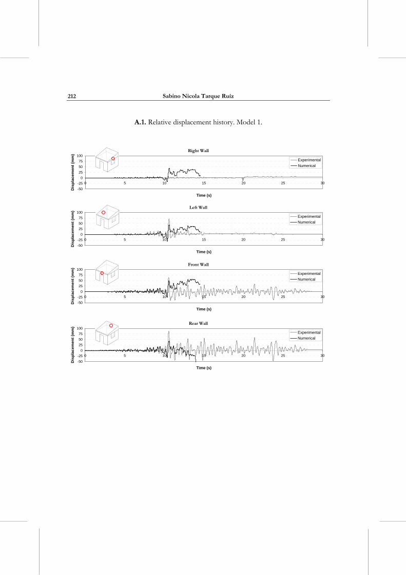
Sabino Nicola Tarque Ruíz
212
A.1. Relative displacement history. Model 1.
Right Wall
-50
-25
0
25
50
75
100
0 5 10 15 20 25 30
Time (s)
Dis
pla
cem
ent
(mm
)
Experimental
Numerical
Left Wall
-50
-25
0
25
50
75
100
0 5 10 15 20 25 30
Time (s)
Dis
pla
cem
ent
(mm
)
Experimental
Numerical
Front Wall
-50
-25
0
25
50
75
100
0 5 10 15 20 25 30
Time (s)
Dis
pla
cem
en
t (m
m)
Experimental
Numerical
Rear Wall
-50
-25
0
25
50
75
100
0 5 10 15 20 25 30
Time (s)
Dis
pla
cem
ent
(mm
)
Experimental
Numerical
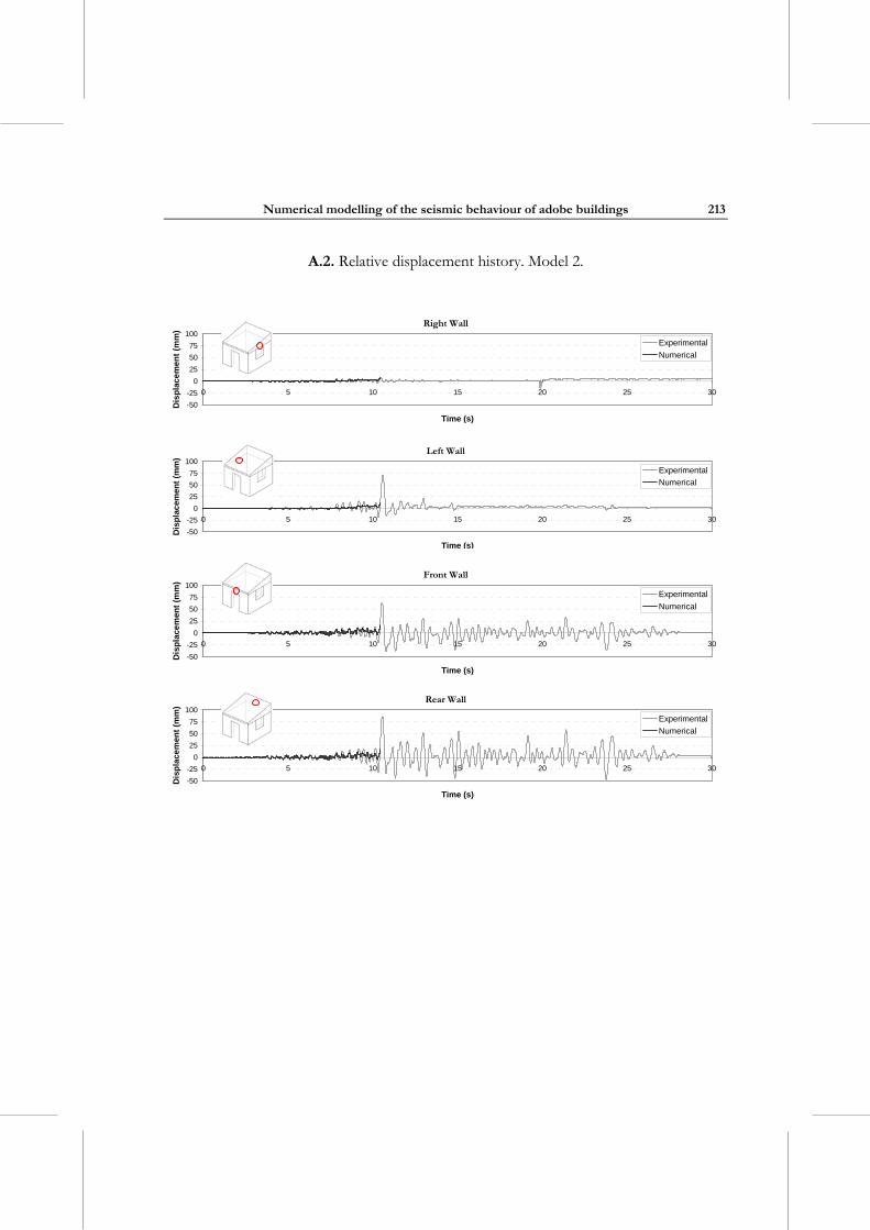
Numerical modelling of the seismic behaviour of adobe buildings
213
A.2. Relative displacement history. Model 2.
Right Wall
-50
-25
0
25
50
75
100
0 5 10 15 20 25 30
Time (s)
Dis
pla
ce
men
t (m
m)
Experimental
Numerical
Left Wall
-50
-25
0
25
50
75
100
0 5 10 15 20 25 30
Time (s)
Dis
pla
cem
ent
(mm
)
Experimental
Numerical
Front Wall
-50
-25
0
25
50
75
100
0 5 10 15 20 25 30
Time (s)
Dis
pla
cem
ent
(mm
)
Experimental
Numerical
Rear Wall
-50
-25
0
25
50
75
100
0 5 10 15 20 25 30
Time (s)
Dis
pla
cem
ent
(mm
)
Experimental
Numerical
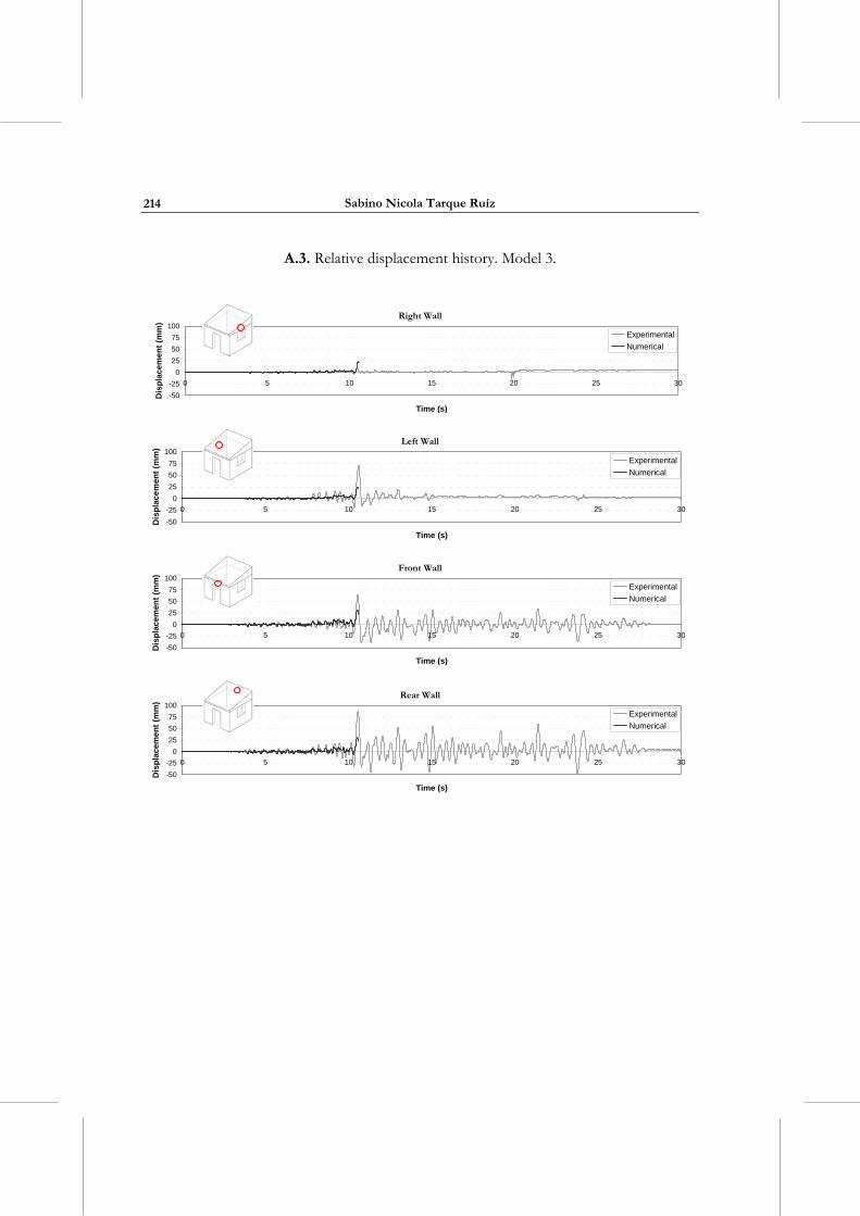
Sabino Nicola Tarque Ruíz
214
A.3. Relative displacement history. Model 3.
Right Wall
-50
-25
0
25
50
75
100
0 5 10 15 20 25 30
Time (s)
Dis
pla
cem
ent
(mm
)
Experimental
Numerical
Left Wall
-50
-25
0
25
50
75
100
0 5 10 15 20 25 30
Time (s)
Dis
pla
cem
ent
(mm
)
Experimental
Numerical
Front Wall
-50
-25
0
25
50
75
100
0 5 10 15 20 25 30
Time (s)
Dis
pla
cem
ent
(mm
)
Experimental
Numerical
Rear Wall
-50
-25
0
25
50
75
100
0 5 10 15 20 25 30
Time (s)
Dis
pla
cem
ent
(mm
)
Experimental
Numerical
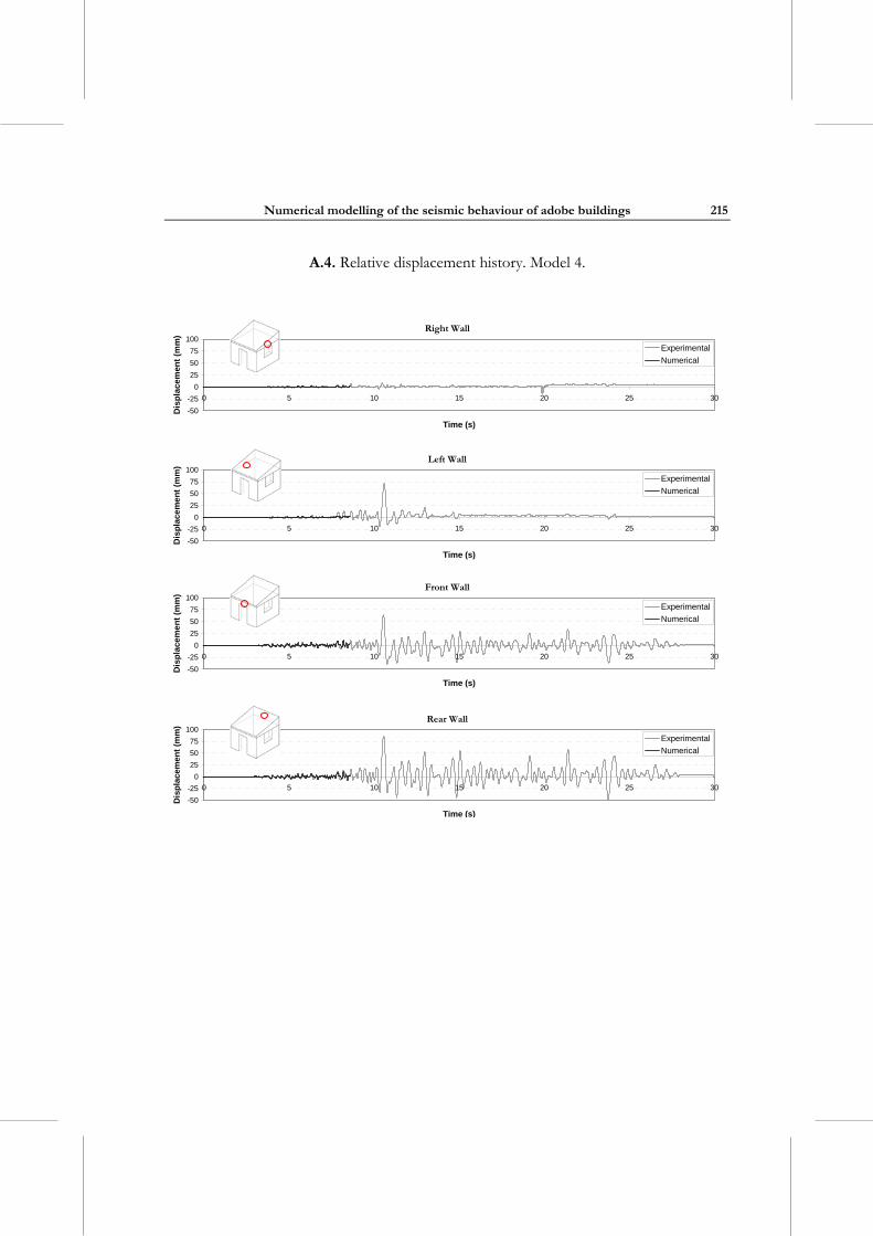
Numerical modelling of the seismic behaviour of adobe buildings
215
A.4. Relative displacement history. Model 4.
Right Wall
-50
-25
0
25
50
75
100
0 5 10 15 20 25 30
Time (s)
Dis
pla
cem
ent
(mm
)
Experimental
Numerical
Left Wall
-50
-25
0
25
50
75
100
0 5 10 15 20 25 30
Time (s)
Dis
pla
cem
en
t (m
m)
Experimental
Numerical
Front Wall
-50
-25
0
25
50
75
100
0 5 10 15 20 25 30
Time (s)
Dis
pla
cem
ent
(mm
)
Experimental
Numerical
Rear Wall
-50
-25
0
25
50
75
100
0 5 10 15 20 25 30
Time (s)
Dis
pla
cem
ent
(mm
)
Experimental
Numerical
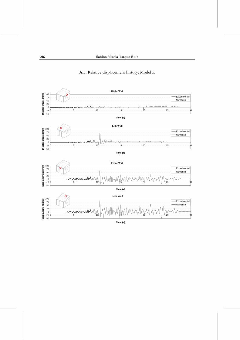
Sabino Nicola Tarque Ruíz
216
A.5. Relative displacement history. Model 5.
Right Wall
-50
-25
0
25
50
75
100
0 5 10 15 20 25 30
Time (s)
Dis
pla
cem
ent
(mm
)
Experimental
Numerical
Left Wall
-50
-25
0
25
50
75
100
0 5 10 15 20 25 30
Time (s)
Dis
pla
cem
ent
(mm
)
Experimental
Numerical
Front Wall
-50
-25
0
25
50
75
100
0 5 10 15 20 25 30
Time (s)
Dis
pla
cem
ent
(mm
)
Experimental
Numerical
Rear Wall
-50
-25
0
25
50
75
100
0 5 10 15 20 25 30
Time (s)
Dis
pla
cem
ent
(mm
)
Experimental
Numerical
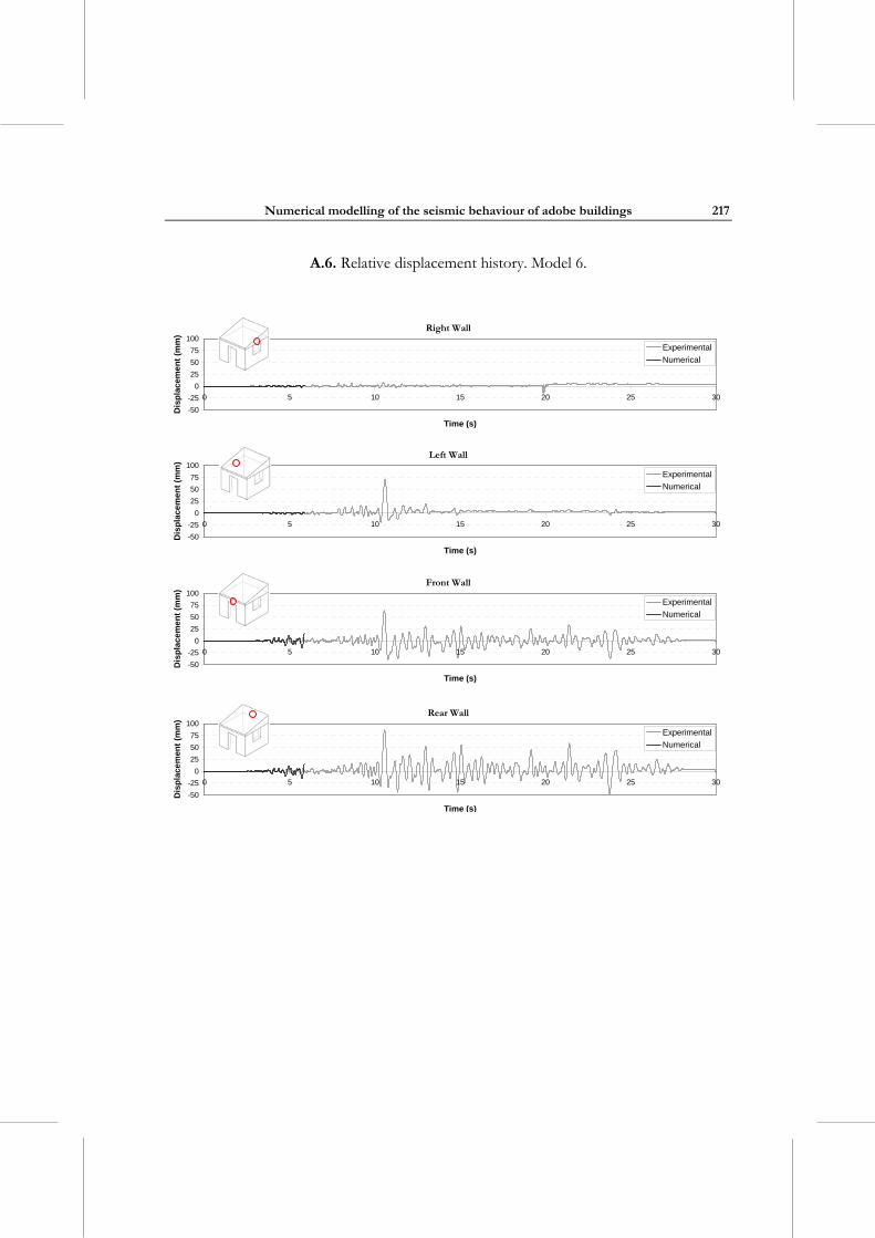
Numerical modelling of the seismic behaviour of adobe buildings
217
A.6. Relative displacement history. Model 6.
Right Wall
-50
-25
0
25
50
75
100
0 5 10 15 20 25 30
Time (s)
Dis
pla
cem
ent
(mm
)
Experimental
Numerical
Left Wall
-50
-25
0
25
50
75
100
0 5 10 15 20 25 30
Time (s)
Dis
pla
cem
ent
(mm
)
Experimental
Numerical
Front Wall
-50
-25
0
25
50
75
100
0 5 10 15 20 25 30
Time (s)
Dis
pla
cem
en
t (m
m)
Experimental
Numerical
Rear Wall
-50
-25
0
25
50
75
100
0 5 10 15 20 25 30
Time (s)
Dis
pla
cem
ent
(mm
)
Experimental
Numerical
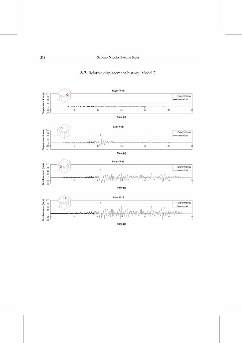
Sabino Nicola Tarque Ruíz
218
A.7. Relative displacement history. Model 7.
Right Wall
-50
-25
0
25
50
75
100
0 5 10 15 20 25 30
Time (s)
Dis
pla
cem
ent
(mm
)
Experimental
Numerical
Left Wall
-50
-25
0
25
50
75
100
0 5 10 15 20 25 30
Time (s)
Dis
pla
cem
ent
(mm
)
Experimental
Numerical
Front Wall
-50
-25
0
25
50
75
100
0 5 10 15 20 25 30
Time (s)
Dis
pla
cem
ent
(mm
)
Experimental
Numerical
Rear Wall
-50
-25
0
25
50
75
100
0 5 10 15 20 25 30
Time (s)
Dis
pla
cem
ent
(mm
)
Experimental
Numerical
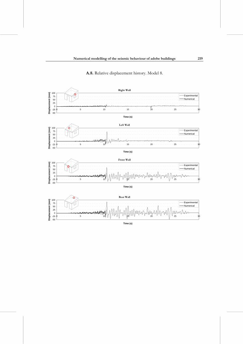
Numerical modelling of the seismic behaviour of adobe buildings
219
A.8. Relative displacement history. Model 8.
Right Wall
-50
-25
0
25
50
75
100
0 5 10 15 20 25 30
Time (s)
Dis
pla
cem
en
t (m
m)
Experimental
Numerical
Left Wall
-50
-25
0
25
50
75
100
0 5 10 15 20 25 30
Time (s)
Dis
pla
cem
ent
(mm
)
Experimental
Numerical
Front Wall
-50
-25
0
25
50
75
100
0 5 10 15 20 25 30
Time (s)
Dis
pla
cem
ent
(mm
)
Experimental
Numerical
Rear Wall
-50
-25
0
25
50
75
100
0 5 10 15 20 25 30
Time (s)
Dis
pla
cem
ent
(mm
)
Experimental
Numerical


APPENDIX B. Comparison of the experimental and
numerical total acceleration response of the adobe module.
Implicit analysis.
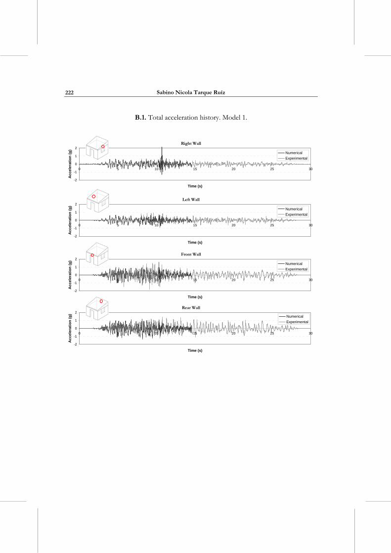
Sabino Nicola Tarque Ruíz
222
B.1. Total acceleration history. Model 1.
Right Wall
-2
-1
0
1
2
0 5 10 15 20 25 30
Time (s)
Ac
cele
rati
on
(g
)
Numerical
Experimental
Left Wall
-2
-1
0
1
2
0 5 10 15 20 25 30
Time (s)
Acc
eler
ati
on
(g
)
Numerical
Experimental
Front Wall
-2
-1
0
1
2
0 5 10 15 20 25 30
Time (s)
Ac
cele
rati
on
(g
)
Numerical
Experimental
Rear Wall
-2
-1
0
1
2
0 5 10 15 20 25 30
Time (s)
Ac
cele
rati
on
(g
)
Numerical
Experimental
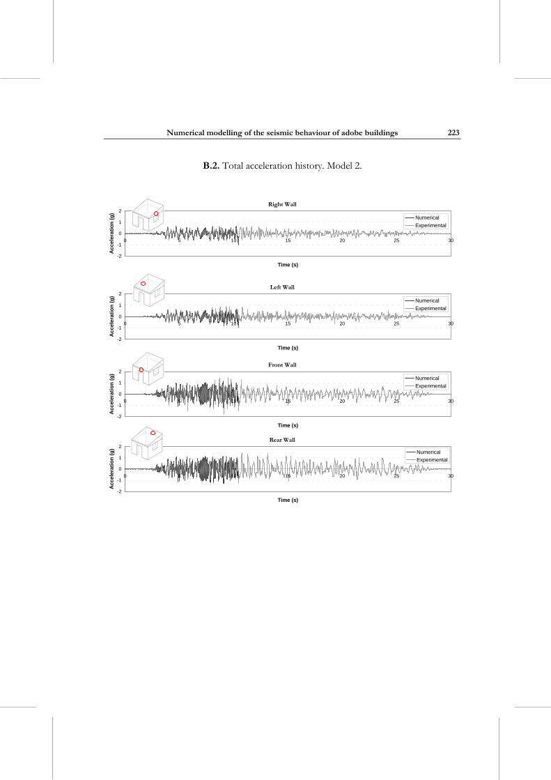
Numerical modelling of the seismic behaviour of adobe buildings
223
B.2. Total acceleration history. Model 2.
Right Wall
-2
-1
0
1
2
0 5 10 15 20 25 30
Time (s)
Ac
cele
rati
on
(g
)
Numerical
Experimental
Left Wall
-2
-1
0
1
2
0 5 10 15 20 25 30
Time (s)
Ac
cele
rati
on
(g
)
Numerical
Experimental
Front Wall
-2
-1
0
1
2
0 5 10 15 20 25 30
Time (s)
Acc
eler
ati
on
(g
)
Numerical
Experimental
Rear Wall
-2
-1
0
1
2
0 5 10 15 20 25 30
Time (s)
Acc
ele
rati
on
(g
)
Numerical
Experimental
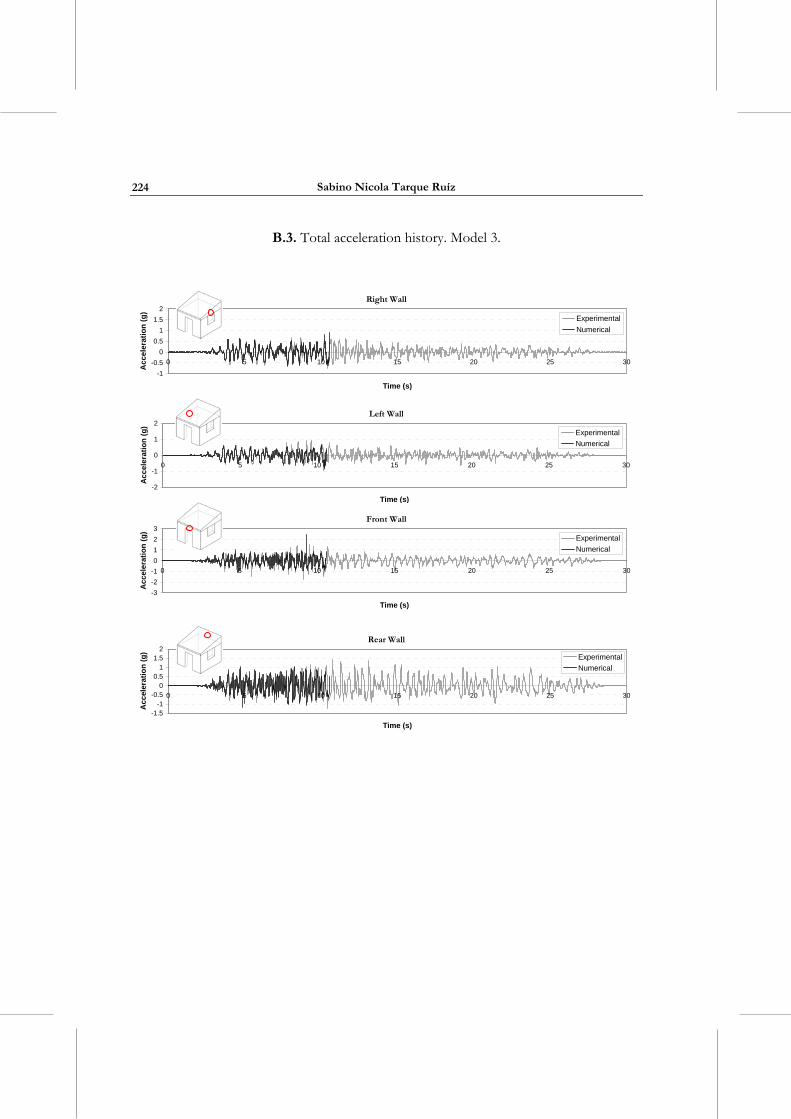
Sabino Nicola Tarque Ruíz
224
B.3. Total acceleration history. Model 3.
Right Wall
-1
-0.5
0
0.5
1
1.5
2
0 5 10 15 20 25 30
Time (s)
Ac
cele
rati
on
(g
)
Experimental
Numerical
Left Wall
-2
-1
0
1
2
0 5 10 15 20 25 30
Time (s)
Acc
eler
atio
n (
g)
Experimental
Numerical
Front Wall
-3
-2
-1
0
1
2
3
0 5 10 15 20 25 30
Time (s)
Acc
eler
atio
n (
g)
Experimental
Numerical
Rear Wall
-1.5-1
-0.50
0.51
1.52
0 5 10 15 20 25 30
Time (s)
Acc
eler
atio
n (
g)
Experimental
Numerical
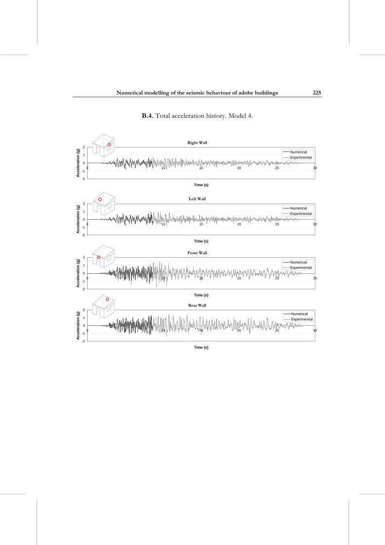
Numerical modelling of the seismic behaviour of adobe buildings
225
B.4. Total acceleration history. Model 4.
Right Wall
-2
-1
0
1
2
0 5 10 15 20 25 30
Time (s)
Ac
cele
rati
on
(g
)
Numerical
Experimental
Left Wall
-2
-1
0
1
2
0 5 10 15 20 25 30
Time (s)
Ac
cele
rati
on
(g
)
Numerical
Experimental
Front Wall
-2
-1
0
1
2
0 5 10 15 20 25 30
Time (s)
Acc
eler
ati
on
(g
)
Numerical
Experimental
Rear Wall
-2
-1
0
1
2
0 5 10 15 20 25 30
Time (s)
Acc
ele
rati
on
(g
)
Numerical
Experimental
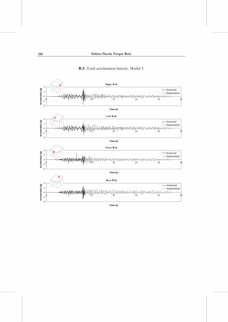
Sabino Nicola Tarque Ruíz
226
B.5. Total acceleration history. Model 5.
Right Wall
-2
-1
0
1
2
0 5 10 15 20 25 30
Time (s)
Ac
cele
rati
on
(g
)
Numerical
Experimental
Left Wall
-2
-1
0
1
2
0 5 10 15 20 25 30
Time (s)
Ac
cele
rati
on
(g
)
Numerical
Experimental
Front Wall
-4
-2
0
2
4
0 5 10 15 20 25 30
Time (s)
Ac
cele
rati
on
(g
)
Numerical
Experimental
Rear Wall
-4
-2
0
2
4
0 5 10 15 20 25 30
Time (s)
Acc
eler
atio
n (
g)
Numerical
Experimental
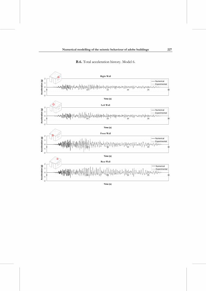
Numerical modelling of the seismic behaviour of adobe buildings
227
B.6. Total acceleration history. Model 6.
Right Wall
-2
-1
0
1
2
0 5 10 15 20 25 30
Time (s)
Ac
cel
era
tio
n (
g)
Numerical
Experimental
Left Wall
-2
-1
0
1
2
0 5 10 15 20 25 30
Time (s)
Ac
cele
rati
on
(g
)
Numerical
Experimental
Front Wall
-2
-1
0
1
2
0 5 10 15 20 25 30
Time (s)
Acc
eler
atio
n (
g)
Numerical
Experimental
Rear Wall
-2
-1
0
1
2
0 5 10 15 20 25 30
Time (s)
Acc
ele
rati
on
(g
)
Numerical
Experimental
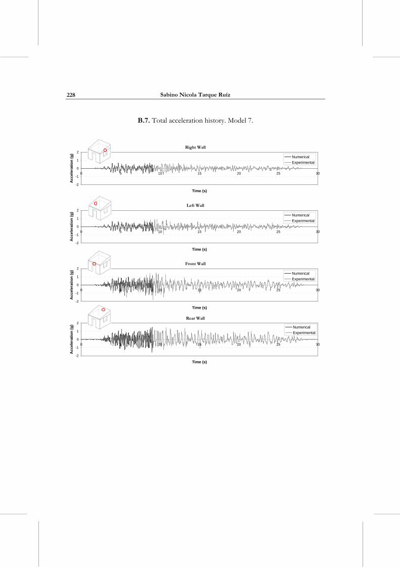
Sabino Nicola Tarque Ruíz
228
B.7. Total acceleration history. Model 7.
Right Wall
-2
-1
0
1
2
0 5 10 15 20 25 30
Time (s)
Acc
eler
atio
n (
g)
Numerical
Experimental
Left Wall
-2
-1
0
1
2
0 5 10 15 20 25 30
Time (s)
Ac
cele
rati
on
(g
)
Numerical
Experimental
Front Wall
-2
-1
0
1
2
0 5 10 15 20 25 30
Time (s)
Acc
eler
ati
on
(g
)
Numerical
Experimental
Rear Wall
-2
-1
0
1
2
0 5 10 15 20 25 30
Time (s)
Acc
ele
rati
on
(g
)
Numerical
Experimental
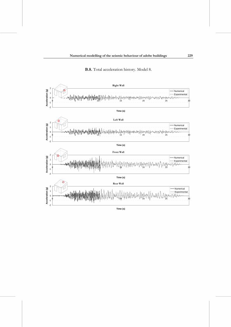
Numerical modelling of the seismic behaviour of adobe buildings
229
B.8. Total acceleration history. Model 8.
Right Wall
-2
-1
0
1
2
0 5 10 15 20 25 30
Time (s)
Acc
eler
atio
n (
g)
Numerical
Experimental
Left Wall
-2
-1
0
1
2
0 5 10 15 20 25 30
Time (s)
Ac
cele
rati
on
(g
)
Numerical
Experimental
Front Wall
-2
-1
0
1
2
0 5 10 15 20 25 30
Time (s)
Acc
eler
ati
on
(g
)
Numerical
Experimental
Rear Wall
-2
-1
0
1
2
0 5 10 15 20 25 30
Time (s)
Acc
ele
rati
on
(g
)
Numerical
Experimental


APPENDIX C. Comparison of the experimental and
numerical relative displacement response of the adobe
module. Explicit analysis.
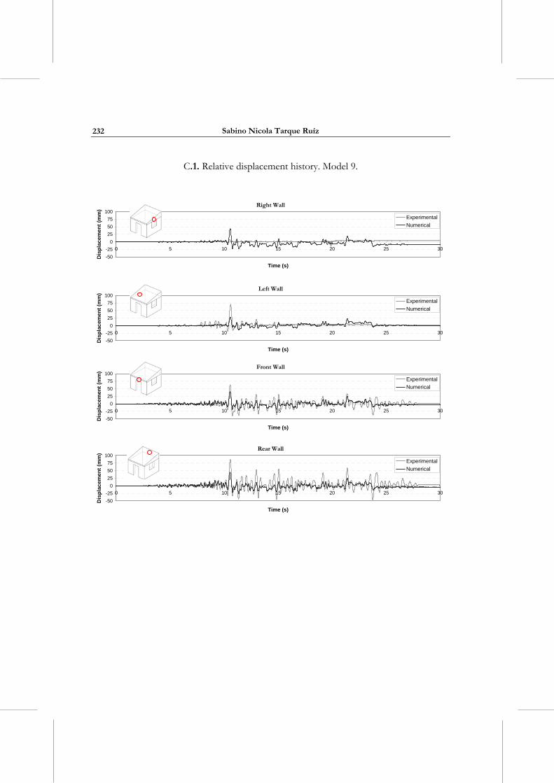
Sabino Nicola Tarque Ruíz
232
C.1. Relative displacement history. Model 9.
Right Wall
-50
-25
0
25
50
75
100
0 5 10 15 20 25 30
Time (s)
Dis
pla
cem
ent
(mm
)
Experimental
Numerical
Left Wall
-50
-25
0
25
50
75
100
0 5 10 15 20 25 30
Time (s)
Dis
pla
cem
en
t (m
m)
Experimental
Numerical
Front Wall
-50
-25
0
25
50
75
100
0 5 10 15 20 25 30
Time (s)
Dis
pla
cem
en
t (m
m)
Experimental
Numerical
Rear Wall
-50
-25
0
25
50
75
100
0 5 10 15 20 25 30
Time (s)
Dis
pla
cem
ent
(mm
)
Experimental
Numerical
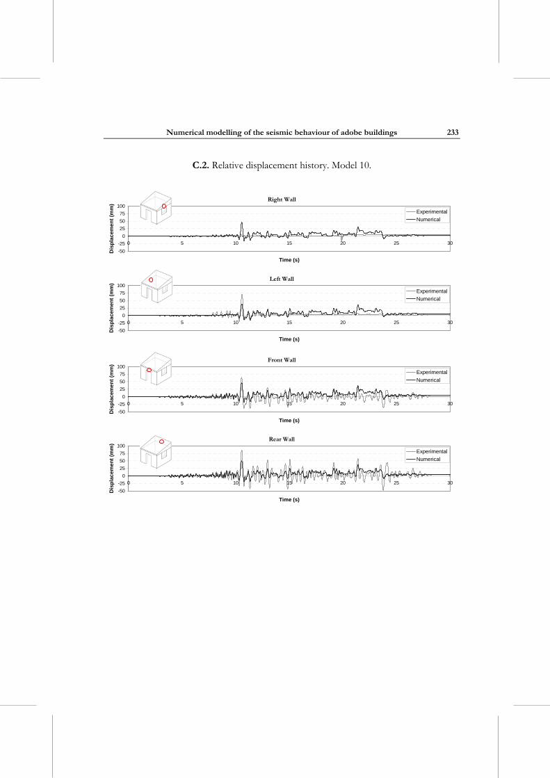
Numerical modelling of the seismic behaviour of adobe buildings
233
C.2. Relative displacement history. Model 10.
Right Wall
-50
-25
0
25
50
75
100
0 5 10 15 20 25 30
Time (s)
Dis
pla
cem
ent
(mm
)
Experimental
Numerical
Left Wall
-50
-25
0
25
50
75
100
0 5 10 15 20 25 30
Time (s)
Dis
pla
cem
ent
(mm
)
Experimental
Numerical
Front Wall
-50
-25
0
25
50
75
100
0 5 10 15 20 25 30
Time (s)
Dis
pla
cem
ent
(mm
)
Experimental
Numerical
Rear Wall
-50
-25
0
25
50
75
100
0 5 10 15 20 25 30
Time (s)
Dis
pla
cem
ent
(mm
)
Experimental
Numerical
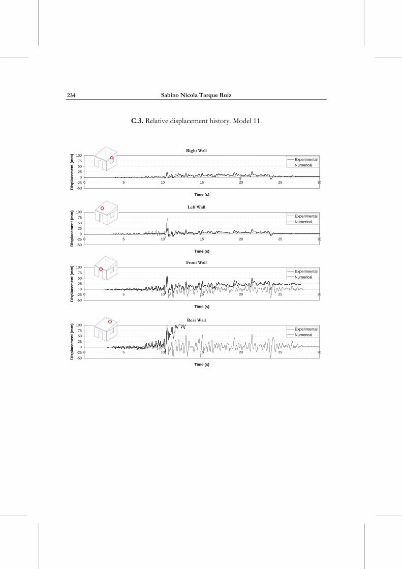
Sabino Nicola Tarque Ruíz
234
C.3. Relative displacement history. Model 11.
Right Wall
-50
-25
0
25
50
75
100
0 5 10 15 20 25 30
Time (s)
Dis
pla
cem
ent
(mm
)
Experimental
Numerical
Left Wall
-50
-25
0
25
50
75
100
0 5 10 15 20 25 30
Time (s)
Dis
pla
cem
ent
(mm
)
Experimental
Numerical
Front Wall
-50
-25
0
25
50
75
100
0 5 10 15 20 25 30
Time (s)
Dis
pla
cem
ent
(mm
)
Experimental
Numerical
Rear Wall
-50
-25
0
25
50
75
100
0 5 10 15 20 25 30
Time (s)
Dis
pla
cem
ent
(mm
)
Experimental
Numerical

Numerical modelling of the seismic behaviour of adobe buildings
235
C.4. Relative displacement history. Model 12.
Right Wall
-50
-25
0
25
50
75
100
0 5 10 15 20 25 30
Time (s)
Dis
pla
cem
ent
(mm
)
Experimental
Numerical
Left Wall
-50
-25
0
25
50
75
100
0 5 10 15 20 25 30
Time (s)
Dis
pla
cem
ent
(mm
)
Experimental
Numerical
Front Wall
-50
-25
0
25
50
75
100
0 5 10 15 20 25 30
Time (s)
Dis
pla
cem
ent
(mm
)
Experimental
Numerical
Rear Wall
-50
-25
0
25
50
75
100
0 5 10 15 20 25 30
Time (s)
Dis
pla
cem
ent
(mm
)
Experimental
Numerical
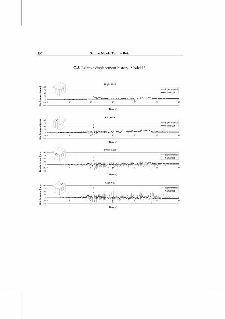
Sabino Nicola Tarque Ruíz
236
C.5. Relative displacement history. Model 13.
Right Wall
-50
-25
0
25
50
75
100
0 5 10 15 20 25 30
Time (s)
Dis
pla
cem
ent
(mm
)
Experimental
Numerical
Left Wall
-50
-25
0
25
50
75
100
0 5 10 15 20 25 30
Time (s)
Dis
pla
cem
ent
(mm
)
Experimental
Numerical
Front Wall
-50
-25
0
25
50
75
100
0 5 10 15 20 25 30
Time (s)
Dis
pla
cem
en
t (m
m)
Experimental
Numerical
Rear Wall
-50
-25
0
25
50
75
100
0 5 10 15 20 25 30
Time (s)
Dis
pla
cem
ent
(mm
)
Experimental
Numerical
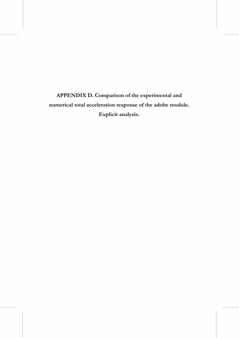
APPENDIX D. Comparison of the experimental and
numerical total acceleration response of the adobe module.
Explicit analysis.
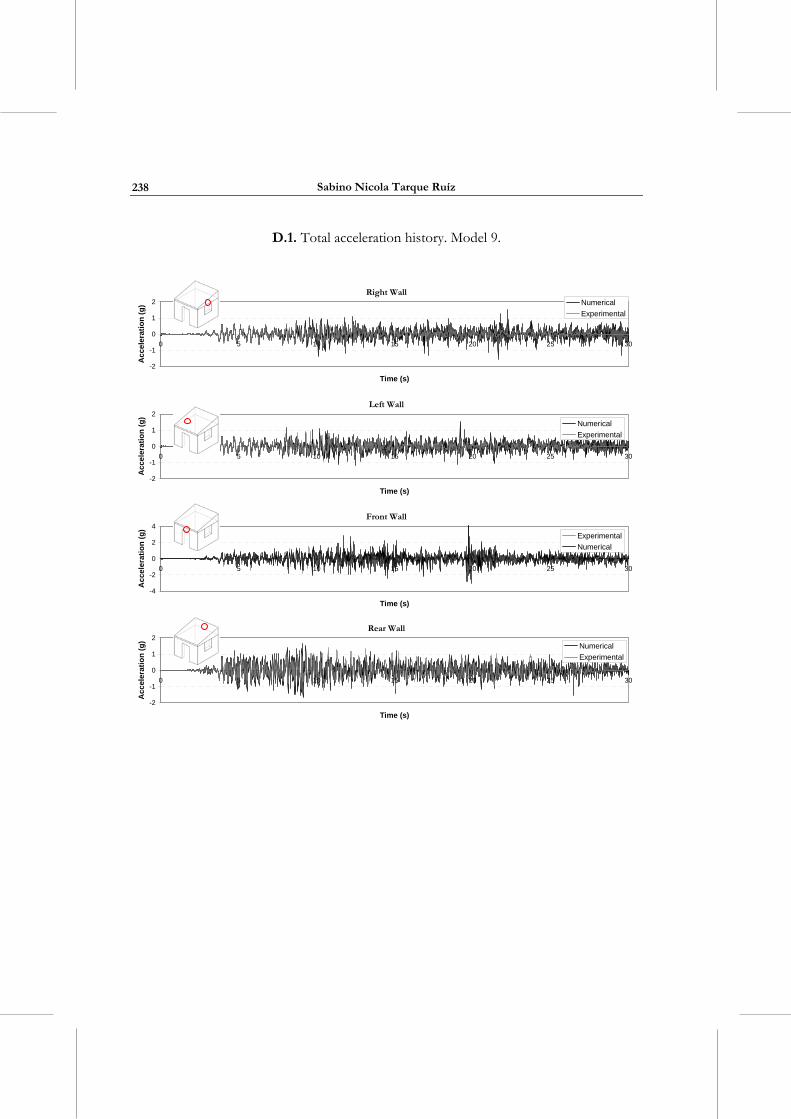
Sabino Nicola Tarque Ruíz
238
D.1. Total acceleration history. Model 9.
Right Wall
-2
-1
0
1
2
0 5 10 15 20 25 30
Time (s)
Ac
cele
rati
on
(g
) Numerical
Experimental
Left Wall
-2
-1
0
1
2
0 5 10 15 20 25 30
Time (s)
Ac
cele
rati
on
(g
)
Numerical
Experimental
Front Wall
-4
-2
0
2
4
0 5 10 15 20 25 30
Time (s)
Acc
ele
rati
on
(g
)
Experimental
Numerical
Rear Wall
-2
-1
0
1
2
0 5 10 15 20 25 30
Time (s)
Ac
cel
era
tio
n (
g)
Numerical
Experimental
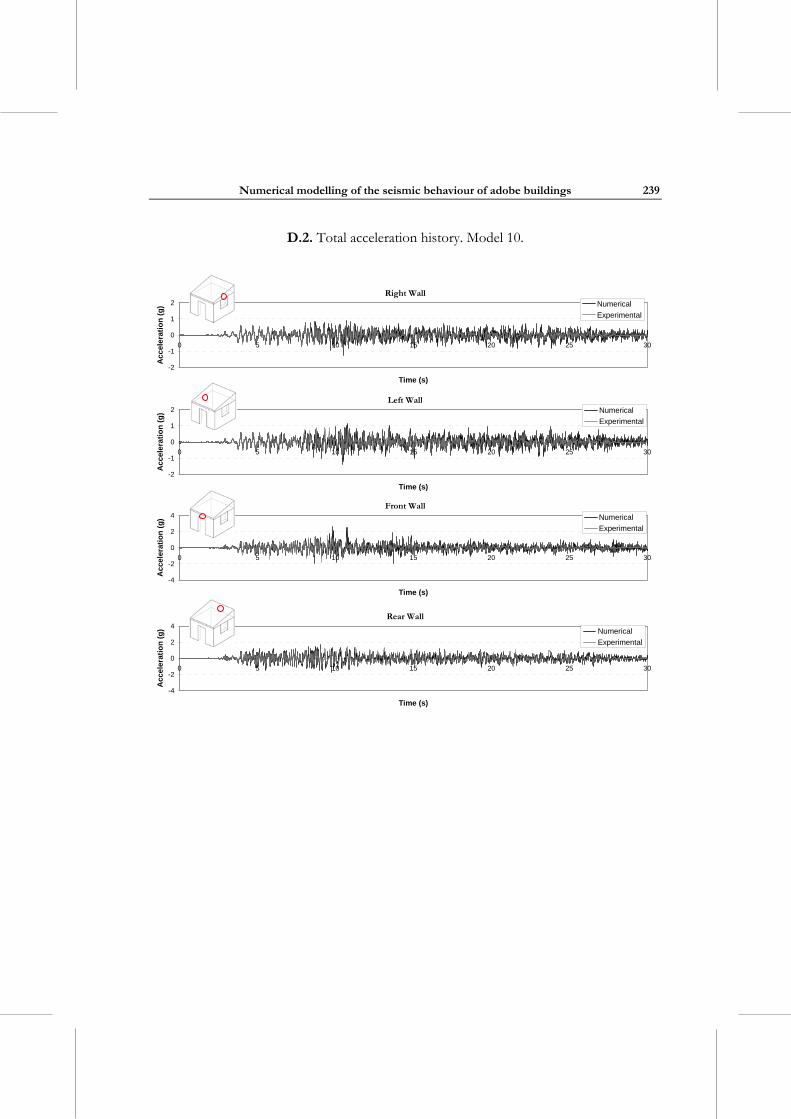
Numerical modelling of the seismic behaviour of adobe buildings
239
D.2. Total acceleration history. Model 10.
Right Wall
-2
-1
0
1
2
0 5 10 15 20 25 30
Time (s)
Ac
cele
rati
on
(g
) Numerical
Experimental
Left Wall
-2
-1
0
1
2
0 5 10 15 20 25 30
Time (s)
Ac
cele
rati
on
(g
) Numerical
Experimental
Front Wall
-4
-2
0
2
4
0 5 10 15 20 25 30
Time (s)
Ac
cele
rati
on
(g
) Numerical
Experimental
Rear Wall
-4
-2
0
2
4
0 5 10 15 20 25 30
Time (s)
Acc
ele
rati
on
(g
) Numerical
Experimental
Sabino Nicola Tarque Ruíz
240
D.3. Total acceleration history. Model 11.
Right Wall
-2
-1
0
1
2
0 5 10 15 20 25 30
Time (s)
Ac
cele
rati
on
(g
) Numerical
Experimental
Left Wall
-2
-1
0
1
2
0 5 10 15 20 25 30
Time (s)
Ac
cele
rati
on
(g
) Numerical
Experimental
Front Wall
-4
-2
0
2
4
0 5 10 15 20 25 30
Time (s)
Acc
eler
ati
on
(g
) Numerical
Experimental
Rear Wall
-4
-2
0
2
4
0 5 10 15 20 25 30
Time (s)
Ac
cele
rati
on
(g
) Numerical
Experimental
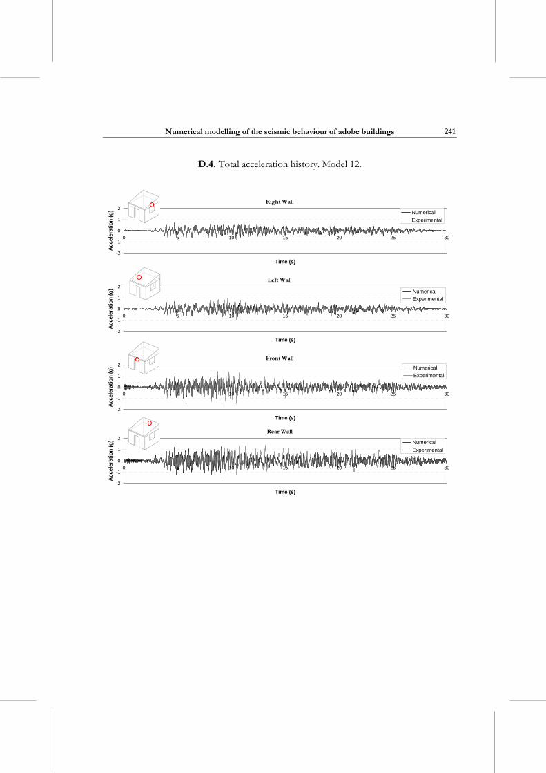
Numerical modelling of the seismic behaviour of adobe buildings
241
D.4. Total acceleration history. Model 12.
Right Wall
-2
-1
0
1
2
0 5 10 15 20 25 30
Time (s)
Ac
cele
rati
on
(g
) Numerical
Experimental
Left Wall
-2
-1
0
1
2
0 5 10 15 20 25 30
Time (s)
Acc
ele
rati
on
(g
) Numerical
Experimental
Front Wall
-2
-1
0
1
2
0 5 10 15 20 25 30
Time (s)
Acc
ele
rati
on
(g
) Numerical
Experimental
Rear Wall
-2
-1
0
1
2
0 5 10 15 20 25 30
Time (s)
Acc
eler
atio
n (
g) Numerical
Experimental
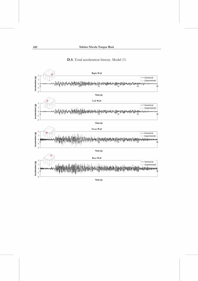
Sabino Nicola Tarque Ruíz
242
D.5. Total acceleration history. Model 13.
Right Wall
-2
-1
0
1
2
0 5 10 15 20 25 30
Time (s)
Ac
cele
rati
on
(g
)
Numerical
Experimental
Left Wall
-2
-1
0
1
2
0 5 10 15 20 25 30
Time (s)
Acc
eler
atio
n (
g)
Numerical
Experimental
Front Wall
-2
-1
0
1
2
0 5 10 15 20 25 30
Time (s)
Acc
ele
rati
on
(g
) Numerical
Experimental
Rear Wall
-2
-1
0
1
2
0 5 10 15 20 25 30
Time (s)
Ac
cel
era
tio
n (
g) Numerical
Experimental