TECHNICAL UNIVERSITY HAMBURG-HARBURGAB - MATHEMATICS

NUMERICAL MODELLING

IN COMPUTATIONAL FLUID DYNAMICS

Maria Lukacova - Medvid’ova

1

CONTENTS

INTRODUCTION 2

Chapter I. BASIC EQUATIONSDESCRIBING FLOWS 5

1.1 Conservation Laws 6

1.2 Constitutive Relations 11

1.3 Thermodynamic State Equations 14

1.4 Boundary and Initial Conditions 16

Chapter II. EULER EQUATIONSAND THEIR NUMERICAL SOLUTION 20

2.1 Theoretical Results 20

2.2 Finite Volume Method 39

2.3 Boundary Conditions 60

2.4 Second Order Method 62

Chapter III. TUTORIALS 70

REFERENCES 76

1

The book of nature is written in the language of mathematics.Galileo Galilei

INTRODUCTION

Mankind has always been attracted by the idea of being able to fly. Flyingseemed to be an unreachable goal, which is clearly exemplified by the myth ofIkarus.

One of the first men who tried to change this situation was famous Leonardoda Vinci. In 1505 he drew the first designs of flying machines with an aviator inhorizontal or vertical position. However he realized that human power was notsufficient to move these flying machines.

Many others tried to continue in this work but they did not succeed. Next 400years it was believed that flying with a motor will not be possible.

The first who actually left the ground were Wright brothers in 1903. The secretof their success was hidden in using of a wind-tunnel in the design of their aeroplane.

From this time the using of wind-tunnels for experimental purposes increases.During the Second World War the first simple mathematical models were computedon large machines to simulate flow problems.

Nowadays Computational Fluid Dynamics (CFD) plays an important role. Dueto the development of highly efficient computers we are able to obtain the behaviourof a flow passing any part of machine. This allows us to choose the best numericaldesign of plane which is then experimentally tested.

But the application of CFD does not lie only in the aeroplane industry. Liquidshave also very similar behaviour as gases, and CFD techniques are used for study ofmotion of water, blood or oil. We can meet its application in the design of turbines,constructions of ships, oil pipelines, channels or in special part of medicine, dealingwith flow of blood, hemodynamics.

To the long list of applications of CFD we can add one more that is very impor-tant from theoretical point of view. There are still some open theoretical problemsconcerning the fundamental questions on existence and uniqueness of a solution toequations describing the motion of fluids. Numerical experiments can help us tounderstand behaviour of various types of flows and to give at least some “verified”hypothesis concerning the answers to these open problems.

This scriptum is devoted to the study of numerical solution of inviscid com-pressible flow. It is governed by the system of conservation laws consisting of thecontinuity equation, the Euler equations of motion of inviscid flow, the energy equa-tion and the state equation. If the viscous effects are included we get the so-called

2

Navier-Stokes equations. Nowadays there are well-developed numerical techniques,such as the finite volume methods, and finite element methods, which play an im-portant role for mathematical and engineering modelling of technical problems.

The aim of this scriptum is to give an introduction and brief description of sev-eral numerical techniques used in the computational fluid dynamics of compressibleinviscid flows. These lecture notes were developed from my notes on MathematicalMethods in Fluid Dynamics, which I have taught at the Mathematical Institute,University of Technology in Brno for students of mathematical engineering (9th se-mester). The overall emphasis of this notes is on studying the mathematical toolsthat are essential in developing, analyzing, and successfully using numerical meth-ods for nonlinear systems of conservation laws, particularly for inviscid problemsinvolving shock waves. An understanding of mathematical structure of the gov-erning equations is first required. Afterwards a reasonable scheme for solving thesystem of partial differential equations can be suggested and studied. In this notesI have stressed the underlying ideas used in various classes of methods rather thanpresenting the most sophisticated methods in great details. My aim was to pro-vide a sufficient background that students could then approach the current researchliterature with the necessary tools for understanding.

Some sections have been reworked several times by now, some are still prelimi-nary. I can only hope that the errors will not cause misunderstanding. I hope ofeventually expanding the presented notes into a book, going in deep discussions insome areas. For these reasons I am interested in receiving suggestions, commentsand corrections. I can be reached via email at lukacova@tu-harburg.de.

This notes are organized as follows. In Chapter I we will introduce some basicnotation and physical quantities describing the motion of fluids. We will formulatethe system of conservation laws which govern inviscid as well as viscous compressibleflow.

In Chapter II we will deal with the Euler equations. We summarize knowntheoretical results for existence and uniqueness for hyperbolic conservations laws.Particularly, we deal with multidimensional scalar equation and one-dimensionalsystem. Further we study the specific so-called Riemann problem for linear as wellas nonlinear systems.

For numerical solution, the finite volume method (FVM), applied on fully un-structured grid consisting of the so-called dual finite volumes, is used. We willdiscuss typical problems of finding the weak solution satisfying the entropy in-equality. This is in a close relation to the second law of thermodynamics. Further,we will present results of numerical experiments where the Vijayasundaram FVMis used to compute the Euler equations in 2D. We will particularly discuss someimprovements obtained by the second order TVD-MUSCL Vijayasundaram schemeand by the suitable mesh refinement. There is a wide class of literature concern-ing hyperbolic conservation laws and/or their numerical solution. See, e.g., [Feis-tauer], [Godlewski, Raviart(1),(2)], [Hirsch], [Kroner], [LeVeque(1)], [LeVeque(2)],[Morton, Mayers], [Smoller], [Sonar(1),(2)], [Toro], [Warnecke] to mention some ofthem.

3

In Chapter III we will give a list of unsolved problems which can be used inseminars and for students’ individual work. Some other problems, which corre-sponds to particular theorems of Chapter I, II were already included therein.

Finally I would like to thank Alexander Zenısek, Technical University Brno, forhis support and encouragement in writing these lecture notes. They were furtherdeveloped during my visiting Sofia-Kovalevskaja professorship at the Institute ofComputational Mathematics, University of Kaiserslautern. I want to express mythank to Helmut Neunzert for initiating a valuable project of Sofia-Kovalevskajaprofessorship in order to support female mathematicians. I also wish to thank LiborCermak and Jitka Saibertova, Technical University Brno, for reading of several ver-sions of the manuscripts, fruitful discussions and helpful comments which improvedthe final version of the notes substantially.

I want to express my thanks to my academic teacher, Miloslav Feistauer, CharlesUniversity Prague, for introducing me to a fascinated field of mathematical and nu-merical modelling in fluid dynamics. Further, I want to express my deep thank toGerald Warnecke, Otto-von-Guericke-Univeritat Magdeburg for the hours he de-voted me in various discussions, for his continual support and encouragement. Ialso wish to thank Bill Morton, Bath/Oxford Universities, for his valuable advices,informations and fruitful discussions.

At the end I would like to thank my husband L’ubo and my parents for theirunfailing support, great patience and intuitive understanding of my work.

Hamburg, summer 2003 Maria Lukacova

4

CHAPTER I

BASIC EQUATIONS DESCRIBING FLOWS

Throughout this scriptum we will deal with the complete system of equationsdescribing the motion of compressible viscous and inviscid fluids. In this chapterwe will give physical and mathematical formulation of conservation laws, whichaccompanied by the constitutive relations and thermodynamical state equationslead to the system of Navier–Stokes or Euler equations describing the motion ofviscous or inviscid fluids, respectively. We will formulate the initial-boundary valueproblems for considered compressible flows.

At the beginning we write a list of some symbols and notations we will use:

Ω ⊂ Rd . . . bounded domain occupied by the fluidd ∈ N . . . dimension, in practice d = 2,3〈0, T 〉 . . . time interval, T > 0x = (x1, . . . , xd) ∈ Ω . . . any point from Ωt ∈ 〈0, T 〉 . . . time instant from time interval 〈0, T 〉QT = Ω × (0, T ) . . . space-time cylinderv = v (x, t) = (v1, . . . , vd) . . . velocity vectorρ = ρ (x, t) . . . densityp = p (x, t) . . . pressureθ = θ (x, t) . . . absolute temperatureε = ε (x, t) . . . total specific energy

i.e. per unit of massf = f (x, t) = (f1, . . . , fd) . . . vector of external (volume) forces

per unit of mass (given)q = q (x, t) . . . rate of external heat sources (given)q = q (x, t) . . . heat flux.

These are basic physical quantities describing the moving fluid, other quantitieswill be defined later. Let us note that we will often use the summation convention,i.e. one has to sum up over the index occurring twice in some term. We will recalla well-known definition of the following operators.

For a vector function u = (u1, . . . , un) : Rm → Rn we put

grad ui :=( ∂ui

∂x1, . . . ,

∂ui

∂xm

), i = 1, 2, . . . n;

grad u := ( grad u1, . . . , grad un)T,

5

( note that grad u is an n×m matrix, having in the i-th row a vector grad ui )

if m = n then div u :=n∑

i=1

∂ui

∂xi.

In what follows we will assume that the students are familiar with definitionsand properties of Lp -spaces, Sobolev spaces and Bochner spaces. There is a lotof literature concerning these topics (see, e.g., [Feistauer] [Kufner, Fucık, John],[Malek, Necas, Rokyta, Ruzicka, [Necas], [Zenısek], etc.).

1.1 Conservation Laws

Eulerian and Lagrangian description of fluid motion

Consider the motion of each particular fluid particle. Trajectories of the particlescan be described by the equation

x = ϕ(X, t).

Here X = (X1, . . . , Xd) represents the reference of the particle that we consider.Thus, in d-dimensional space we have together with time variable the following so-called Lagrangian coordinates X, t. The above equation determinates the positionof the particle given by the reference X at time t.

However, if we investigate fluid we are rarely interested in the motion of eachparticular fluid particle. Instead we are interested in the state of flow and its changein time. Therefore, we usually work with the so-called Eulerian coordinates x, t,which are based on the determination of the velocity v(x, t) of the fluid particlepassing through the point x at time t. We can write

v(x, t) =∂ϕ

∂t(X, t),

where x = ϕ(X, t).Now, let us consider some physical quantity F (e.g. temperature, density, etc.)

transported by moving particles in fluid. In the Lagrangian concept this quantityis viewed as F (X, t), which describes the value of the quantity considered, boundto the particular fluid particle given by X at time t.

On the other hand, in the Eulerian description the quantity is represented bya function F (x, t), which denotes the value of quantity at the point x at time t.Describing the path of a fluid particle by the equation x = ϕ(X, t), we can expressthe rate of change of the quantity F (x, t) as

dF (x, t)dt

=dF (ϕ(X, t), t)

dt

=∂F (ϕ(X, t), t)

∂t+

d∑i=1

∂F

∂xi(ϕ(X, t), t)

∂ϕi(X, t)∂t

=∂F (x, t)

∂t+ v(x, t) · grad F (x, t).

6

We see that the rate of change of the quantity F is equal to the so-called materialderivative

d

dtF (x, t) :=

∂F

∂t(x, t) +

d∑i=1

∂F

∂xivi (x, t) .

The local derivative ∂F/∂t results from the dependence of F on time, the convectivederivative v ·grad F is a consequence of the transport of the quantity F by movingfluid. In this context the material derivative is also sometimes called the derivativealong a trajectory of a fluid particle.

Transport theorem

Let us consider transport of the physical quantity F (x, t) (Eulerian description)in a control volume σ(t). The total amount of the quantity given by the functionF that is contained in the volume σ(t) at time t equals

F(t) =∫

σ(t)

F (x, t)dx.

In what follows we will need to calculate the rate of change of the quantity F boundon the system of particles considered. Thus, we are interested in

dF(t)dt

=d

dt

∫σ(t)

F (x, t)dx.

In textbooks of mathematical analysis one can find theorems for differentiation ofintegrals with respect to a parameter, but the domain is fixed. In our situationhowever we have both the integrand F as well as the integration domain σ(t)depending on t. Therefore we need to use the Reynolds transport theorem.

Theorem 1.1.1. Let F : Rd × R → R be a continuously differentiable functionand the mapping ϕ : Rd → Rd be also continuously differentiable. Then for eachcontrol volume σ(t) the following equality holds

dF(t)dt

=d

dt

∫σ(t)

F (x, t)dx =

=∫

σ(t)

[∂F

∂t(x, t) + v(x, t) · grad F (x, t) + F (x, t) div v(x, t)

]dx.

(1.1.2)

Proof. (see, e.g., [Feistauer], [Warnecke]).�

Flux formulation of the transport theorem

It is clear that identity (1.1.2) can be rewritten in the form

dF(t)dt

=∫

σ(t)

[∂F

∂t(x, t) + div (Fv)(x, t)

]dx.

7

By Green’s theorem we get

dF(t)dt

=∫

σ(t)

∂F

∂t(x, t) +

∫∂σ(t)

F (x, t)v(x, t) · n(x)dS,

where n(x) denotes a unit outer normal to ∂σ(t) at the point x. The first integralon the right-hand side determines the rate of change of the quantity F in virtue ofthe dependence of F on t. The second integral represents the flux of the quantity Fthrough the boundary ∂σ(t).

Formulation of basic conservation laws

The first physical law describing the fluid motion is the law of conservation ofmass and can be formulated in the following way:

The mass of a piece of fluid formed by the same particles at any time instant isconstant in time. In other words : mass is neither created nor destroyed.

Let ρ(x, t) be the density of the fluid at a position x and time t. Then the massm(σ(t)) of fluid occupying the control volume σ(t) is given as

∫σ(t)

ρ(x, t)dx. Thefact that the mass is constant in time naturally means that

d

dt

∫σ(t)

ρ(x, t)dx = 0.

Using the Transport theorem 1.1.1 with F = ρ we get under the assumptions onsmooth density ρ ∫

σ(t)

[∂ρ

∂t+ div (ρv)

]= 0.

But the above integral identity holds for any control volume σ(t) ⊂ Ω, where Ω ∈ Rd

is a fixed domain occupied by the fluid, t ∈ (0, T ). Thus the integrand must beequal to zero itself. Now the differential form of the mass conservation, also calledthe continuity equation, reads

(1.1.3)∂ρ

∂t+ div (ρv) = 0 in Ω × (0, T ) .

Incompressible flow

An incompressible flow is a flow in which density of each material particle remainsthe same during the motion

ρ(ϕ(X, t), t) = ρ(X, 0), X = ϕ(X, 0).

Hencedρ

dt= 0 and because div (ρv) = ρ div v + grad ρ · v we get from (1.1.3) the

incompressibility condition

(1.1.3’) div v = 0.

Sometimes incompressibility is erroneously taken to be a property of the fluidinstead of the flow. But compressibility depends only on the speed of the flow. If

8

the magnitude of the velocity of the flow is of order of the speed of sound in the fluid(≈ 340 m/s in air) the flow is compressible. If the velocity is much smaller than thespeed of sound, incompressibility is a good approximation. It is true than in liquidsflow velocities anywhere near the speed of sound cannot normally be reached, dueto enormous pressures involved and the phenomenon of cavitation.

The balance of momentum is just the second Newton’s law F = ma, where Fdenotes the vector of forces, m stays for the mass and a is the acceleration of thefluid. It can be also formulated as follows

The rate of change of total momentum of a piece of fluid formed by the sameparticles at any time instant is equal to the forces acting on this piece of fluid.

There are two types of forces acting in flows: body forces and surface forces. Abody force acts on a material particle, and is proportional to its mass. Let thedensity of the body force be denoted by f(x, t), e.g. the density of gravity force is(0, 0,−g), g is the acceleration of gravity. Then the body force acting on the fluidin the control volume σ(t) is given as∫

σ(t)

ρf(x, t)dx.

The action of the surface forces can be expressed by means of the stress tensorτττ = (τij)

di,j=1, which results from the inner interactions between fluid volumes

through their boundaries. Thus, the surface forces are expressed in the form∫∂σ(t)

τττ · ndS ≡∫

∂σ(t)

(τττ ijnj)di=1dS.

Note that we have used here the Einstein summation convention in the stress tensorterm, i.e. we sum up over the index j occurring twice in the stress tensor term. Inorder to simplify expressions we will often use this convention in what follows.Now the law of conservation of momentum can be for an arbitrary control volumeσ(t) expressed as follows

d

dt

∫σ(t)

ρvi dx =∫

σ(t)

ρfi dx +∫

∂σ(t)

τijnj dS, i = 1, . . . , d.

Using the Transport theorem 1.1.1 for F = ρvi and the Gauss theorem for thesurface integral of the stress tensor we can rewrite the above identity as∫

σ(t)

∂

∂t(ρvi) +

∂

∂xj(ρvivj) dx =

∫σ(t)

ρfi dx +∫

σ(t)

∂τij

∂xjdx, i = 1, . . . , d.

Since this holds for every control volume σ(t) ⊂ Ω, t ∈ (0, T ) we get the differentialform of the momentum conservation law

(1.1.4)∂

∂t(ρvi) +

∂

∂xj(ρvivj) = ρfi +

∂τij

∂xjin Ω × (0, T ) , i = 1, . . . , d.

In order to specify further properties of the stress tensor we use the balanceof moment of momentum, which says:

9

the rate of change of the moment of momentum of a piece of fluid occupied bythe same particles at any time instant is equal to the sum of the moments of theforces acting on this piece of fluid.

It can be proved (see, e.g., [Gurtin]) that this law is equivalent to the symmetryof the stress tensor τττ , i.e.

τij = τji, i, j = 1, 2, . . . , d.

In order to complete the system of the equations (1.1.3) - (1.1.4) it is necessary torelate the stress tensor to other quantities describing the motion of the fluid. Sucha relation is called the constitutive relation and we will discuss this point in thenext section.

The law of conservation of energy, which is the last conservation law used fordescription of the motion of fluid, follows directly from the first law of thermody-namics:

The rate of change of total energy of a piece of fluid formed by the same particlesat any time instant is equal to the sum of powers of the volume and surface forcesacting on this piece of fluid and to the amount of heat transmitted to this piece offluid. In other words one can say: energy is neither created nor destroyed.

For an arbitrary control volume σ(t) we obtain the following integral formulation

(1.1.5)d

dt

∫σ(t)

ρεdx = W (σ(t)) + Q(σ(t)),

where W is the power of the body and surface forces acting on the fluid volumeσ(t) and Q denotes the rate of heat addition. The total specific energy ε consists ofthe specific internal energy, denoted by u = u (x, t) , and the specific kinetic energy12|v (x, t) |2, where |v| =

(∑di=1 v2

i

)1/2

denotes a usual Euclidean norm of a vector.The power of the body and surface forces can be expressed in the form

W (σ(t)) =∫

σ(t)

ρfividx +∫

∂σ(t)

τjinjvidS =∫

σ(t)

ρfivi +∂

∂xjτjividx.

Assuming that heat is added to each material particle at a rate q per unit of mass,and that there is a heat flux q per unit of area through ∂σ(t), we find

Q(σ(t)) =∫

σ(t)

ρqdx −∫

∂σ(t)

q · ndS =∫

σ(t)

ρq − ∂

∂xiqidx.

Substituting the above expressions into (1.1.5) and applying the Transport theo-rem 1.1.1 on the left-hand side of (1.1.5) we get∫

σ(t)

∂

∂t(ρε) +

∂

∂xi(ρεvi) dx =

∫σ(t)

ρfivi +∂

∂xj(τijvi) + ρq − ∂

∂xiqidx.

Since this hold for every control volume σ(t), we have the differential formulationof the law of conservation of energy

(1.1.6)∂

∂t(ρε) +

∂

∂xi(ρεvi) = ρfivi +

∂

∂xj(τijvi) + ρq − ∂

∂xiqi in Ω× (0, T ) .

10

1.2 Constitutive Relations

Putting (1.1.3), (1.1.4) and (1.1.6) together we see that the number of unknownquantities is larger than the number of equations. To complete the whole systemof conservation laws we have to add some constitutive or closing relations that willspecify our fluids.

The first and natural question is the following one: What is the relation betweenthe stress tensor and other quantities describing the fluid motion? Such a relationis called rheological. The simplest situation is obtained in the case of inviscid fluids,where

(1.2.1) τij = −pδij , i, j,= 1, 2, . . . , d,

here δij is a Kronecker delta.Substituting (1.2.1) into the equations of conservation of momentum (1.1.4) we

derive the Euler equations of motion of ideal, i.e. inviscid, fluids

(1.2.2)∂

∂t(ρvi) +

∂

∂xj(ρvivj) = ρfi −

∂p

∂xi, i = 1, . . . , d.

These equations are written in the conservative form; using the continuity equation(1.1.3) we easily derive the convective form of the Euler equations

(1.2.2’)∂vi

∂t+ vj

∂vi

∂xj= fi −

1ρ

∂p

∂xi, i = 1, . . . , d.

Real fluids are more or less viscous. Under the Newton’s hypothesis of lineardependence of the stress tensor on the deformation velocity tensor e, where

e = (eij)di,j=1 , eij =

12( ∂vi

∂xj+

∂vj

∂xi

),

one can derive the following form of τττ :

τij = −pδij + τVij(1.2.3)

τVij = λ div v δij + 2μeij , i, j = 1, 2, . . . , d.

Here τττV =(τVij

)d

i,j=1is said to be a viscous part of stress tensor. The viscosity

is expressed by μ, λ, the first and second viscosity coefficient, respectively. μ is alsocalled dynamical viscosity coefficient. There is often used the following relation

(1.2.4) 3λ + 2μ = 0, μ ≥ 0,

which is derived from the kinetic theory for one-atomic gas. To simplify the situa-tion we will suppose that viscosity coefficients μ and λ are constant. Note that inmany fluids they can depend on density ρ or temperature θ, but not on pressure p.

Fluids satisfying (1.2.3) are called Newtonian fluids. Examples are gasses andliquid such as water or mercury. But there is a large amount of fluids, for which

11

(1.2.3) do not hold. Such fluids are called non-Newtonian fluids, which are nowa-days studied extensively from the experimental as well as theoretical point of view.Examples of those are polymers or blood.

Substitution of (1.2.3) into the equations of conservation of momentum (1.1.4)gives for i = 1, . . . , d

(1.2.5)∂

∂t(ρvi)+

∂

∂xj(ρvivj) = ρfi−

∂p

∂xi+

∂

∂xi(λdiv v)+

∂

∂xj

(μ

(∂vi

∂xj+

∂vj

∂xi

)).

These are the Navier-Stokes equations, which describe the motion of viscous fluids.Similarly as for the Euler equations (1.2.2) we can write the convective form of theNavier-Stokes equations using the continuity equation (1.1.3)

ρ∂vi

∂t+ρvj

∂vi

∂xj= ρfi−

∂p

∂xi+

∂

∂xi(λdiv v)+

∂

∂xj

(μ

(∂vi

∂xj+

∂vj

∂xi

)), i = 1, . . . , d.

If the flows are incompressible div v = 0 and the above identity yields the Navier-Stokes equations for incompressible flows:

(1.2.5’)∂vi

∂t+ vj

∂vi

∂xj= fi −

1ρ

∂p

∂xi+ νΔvi, i = 1, . . . , d,

where ν = μ/ρ is the so-called kinematic viscosity, assumed to be constant. Theseequations were firstly derived by Navier in 1823 and later by Stokes in 1845. Notethat until now the question of global existence and uniqueness of the solution staysfor d = 3 a great open problem in the theory of partial differential equations.In 2000, the year of mathematics, the Clay Mathematical Institute declared theproblem of existence and regularity of the solution to the Navier-Stokes equationsto be one of the seven greatest open problems in mathematics. For each of themthe Millennium Prize of one-million dollars was offered.

The next constitutive relation is obtained from Fourier’s law

(1.2.6) q = −k grad θ,

where k ≥ 0 is called the heat conductivity and is supposed to be constant.

The Reynolds number and similarity of flowsLet L∗, U∗ and t∗ be typical length, velocity and time scales for a given flow

problem, respectively. We introduce the following dimensionless variables

v′ =vU∗ , x′

i =xi

L∗ , t′ =t

t∗

and rewrite the continuity equation (1.1.3’) and the Navier-Stokes equations (1.2.5’)(of incompressible flow) in the form

∂v′i

∂x′i

= 0(L∗

t∗U∗

)∂v′

i

∂t′+ v′

j

∂v′i

∂x′j

=L∗

U∗2 fi −1

U∗2

1ρ

∂p

∂x′i

+ν

L∗U∗Δv′i, i = 1, . . . , d.

12

Thus, if we set t∗ = L∗/U∗, p′ = p/(ρU∗2), f ′

i = fiL∗/U∗2

, ρ = 1 and ν′ =ν/(L∗U∗), then we the continuity equation and the Navier-Stokes equations havethe same form in the variables with primes as in the original variables withoutprimes.

We define the dimensionless Reynolds number

(1.2.7) Re =1ν′ =

L∗U∗

ν

which play an important role in the theory of similarity flows.The above transformation shows that Re is a measure of the ratio of inertial

(convective) and viscous forces in the flow. This can be seen immediately from theequation (1.2.5’) with 1/Re instead of ν. For Re 1 inertia or convective termdominates, for Re � 1 friction or viscosity term dominates. Both are balanced bythe pressure. This is an example of the convection-diffusion equation. The left-handside represents the transport by convection term vj ∂vi/∂xj , the term 1/Re Δvi

represents transport by diffusion. Many aspects of numerical approximation incomputational fluid dynamics already show up in the numerical analysis of relativelysimple convection-diffusion equation.

Let us consider two flows in geometrically similar domains Ω1 and Ω2 such thatΩ1 is L-times larger than Ω2 (“Ω1 = LΩ2”). We call this flow dynamically similar,if they have the same Reynolds numbers. Then their dimensionless Navier-Stokesequations are identical. Similarity of flows allow us to carry out computationalexperiments on small models and transfer the results to the original real flows. Wesee that the solution to the incompressible Navier-Stokes equation depends actuallyon the single parameter Re only.

What values does Re have in practice?

In the International Civil Aviation Organization Standard Atmosphere, ν = μ/ρ =4.9 · 10−5m2/s at 12.5 km. This gives for the flow over an aircraft wing in cruisecondition at 12.5 km with wing length L = 3 m and velocity U = 900km/h:Re = 1.5 · 107. In a windtunnel experiment at sea level with L = 0.5m andU = 25m/s we obtain Re = 8.3 · 105. For landing aircraft at sea level with L = 3mand U = 220km/h we obtain Re = 1.2 · 107. For a house in a light wind withL = 10m and U = 0.5m/s we have Re = 3.3 · 105. Air circulation in a room withL = 4m and U = 0.1m/s gives Re = 2.7 · 104.

Large ship has Re ≈ 108, small yacht Re ≈ 107 and a small fish only Re ≈104. All these examples have in common that Re 1, which is almost the rulein all environmental and industrial flows. One might think that flow around agiven shape will be quite similar for different values of Re, as long as Re 1.But nothing is farther from the truth! Therefore computational fluid dynamicsplays an important role in the prediction of flow behaviour for full scale of Renumbers. The rich variety of solutions that evolves as Re → ∞ is one of the mostsurprising and interesting features of fluid dynamics, with important consequencesfor technological applications.

A ‘route to chaos’ develops as Re → ∞, resulting in turbulence. Turbulentflow is a complicated example of chaotic dynamical system. The difficulty is thatturbulence is both nonlinear and stochastic. Since turbulence is governed by the

13

Navier-Stokes equations, turbulent flow can be computed from the basic conser-vation principles. But nowadays this is still not feasible for general engineeringcomputations. We will explain this more closely in what follows.

Let U and L be velocity and length scale of large eddies in a turbulent flow,respectively, and let as define the macroscale Reynolds number by

Re = UL/ν.

The length scale of smallest eddies is called the Kolmogorov scale, and is denotedby η. It has been shown by Kolmogorov that η/L = O(Re−3/4). Let us considerflow in a pipe with diameter L. After some computation one can show that awayfrom the pipe wall

η/L ≈ O(Re−21/32), Re =150

Re7/8.

To resolve the Kolmogorov scale, the mesh size h of the computational domainmust satisfy h < η. With h = η/2, we obtain for the number of grid cells inone direction N = L/h ≈ Re21/32, so that the total number of cells for three-dimensional computations is

N3 ≈ Re62/32 ≈ Re2.

Let us take, for example, Re = 105; this give us N3 ≈ 1010 number of mesh cells,which is clearly not feasible on the computer infrastructures available at presentand in the foreseeable future. For complicated geometries and higher Reynoldsnumbers the required number of grid cells is even larger. But at moderate Reynoldsnumbers and in simple geometries direct numerical simulation is a valuable tool forstudying the fundamental properties of turbulence. However, in order to be ableto predict, at least approximately, behaviour of flows at high Reynolds numbersseveral turbulence models have been developed for industrial computations. Inengineering practice in order to achieve computer time and memory requirementsthat are feasible, turbulent flows are generally modelled by the Reynolds-averagedNavier-Stokes equations with, e.g., the so-called k − ε model. See, e.g., [Wesseling]or [Zienkiewicz, Taylor] for more details.

1.3 Thermodynamic State Equations

The relations (1.2.1) , (1.2.3) and (1.2.6) still do not give enough informationto obtain the closed system of conservation laws. Choosing as thermodynamicunknowns the density ρ and the temperature θ, to close the system we must addthe following state equations.

(1.3.1) p = p (ρ, θ) ,14

(1.3.2) u = u (ρ, θ) .

Remind that generally we can also assume λ, μ, k to be functions of ρ and θ, i.e.

(1.3.3) λ = λ (ρ, θ) , μ = μ (ρ, θ) , k = k (ρ, θ) .

As we have already said we will restrict to the case of constant functions.In what follows we will always consider perfect gas, which means that (1.3.1)

can be explicitly written as

(1.3.4) p = R ρ θ.

This equation is called the state equation of perfect gas. R > 0 is the specific gasconstant and it can be expressed in the next form

(1.3.5) R = cp − cv,

where cp and cv are the specific heat at constant pressure and volume, respectively.We assume that cp and cv are constant and it follows from experiments that cp > cv.The quantity

(1.3.6) κ =cp

cv> 1

is called the Poisson adiabatic constant, κ = 1.4 for dry air.Now we will specify the relation (1.3.2). A perfect gas is said to be polytropic, if

(1.3.7) u = cvθ.

We will work with a perfect polytropic gas, i.e. thermodynamic state equations(1.3.4), (1.3.7) hold. Let us note that we have just closed the whole system ofconservation laws describing motion of compressible viscous fluids. We have thesame number of unknown functions as the number of equations, i.e. d + 2. Letρ,v, θ be unknown. Then the system of conservation laws (1.1.3), (1.1.4), and(1.1.6) in which the constitutive relations (1.2.3) , (1.2.6) and thermodynamic stateequations (1.3.4), (1.3.7) are included, can be rewritten in the following form

(1.3.8)∂ρ

∂t+

∂

∂xi(ρvi) = 0;

ρ∂vi

∂t+ ρvj

∂vi

∂xj= ρfi −

∂p

∂xi+

∂

∂xi(λdiv v) +

∂

∂xj(2μeij) , i = 1, 2, . . . , d;

cv

(ρ∂θ

∂t+ ρvgrad θ

)= div (kgrad θ) − pdiv v + λ (div v)2 +

12μ

d∑i,j=1

(∂vi

∂xj+

∂vj

∂xi

)2

+ ρq; in QT ≡ Ω × (0, T ).

15

Since p is a function of ρ, θ, in virtue of the state equation (1.3.4), the system(1.3.8) is closed. We have derived the system of Navier–Stokes equations describingthe motion of viscous compressible fluids. The motion of inviscid compressiblefluids is governed by the Euler equations, which are obtained from (1.3.8), if weput λ = 0 = μ. Note that inviscid fluids are non-heat conductive, thus k = 0.

For incompressible flows system (1.3.8) splits into two separate subsystems. Firstwe have the continuity equation (1.1.3’) with the momentum equations (1.2.2’) or(1.2.5’) for inviscid or viscous fluids, respectively. These are d + 1 equations forunknowns: v = (v1, . . . , vd) and p. Without lost of generality we can put ρ = 1.Next we have the energy equation for unknown temperature θ.

Speaking about thermodynamic relations one should not omit a very importantthermodynamic quantity, namely the entropy, denoted by η (specific entropy). Itis defined by the relation

(1.3.9) θ dη = du + p dV,

where V = 1/ρ is the so-called specific volume. This formula expresses the factthat the internal energy gained by the medium during a change from one state toanother is equal to the heat contributed to the medium plus the work done on themedium by compressive action of pressure forces. (See, e.g., [Courant, Friedrichs]).

For a perfect polytropic gas the entropy η can be expressed in the form (see[Feistauer])

(1.3.10) η = cv lnp/p0

(ρ/ρ0)κ + const.,

where p0, ρ0 > 0 are some fixed values of pressure and density, respectively.There is an important law, the second law of thermodynamics (or the so-called

Clausius–Duhem inequality), which is used for a selection of admissible processes.Differential form of this law is

(1.3.11) ρdη

dt≥ −div

(qθ

)+

ρq

θ.

Every material satisfying (1.3.11) is said to be thermodynamic compatible. Theperfect polytropic gas is such a material.

1.4 Boundary and Initial Conditions

In this section we will formulate the initial-boundary value problems for con-sidered inviscid-viscous flows. It means that the system (1.3.8) will be completedby some boundary and initial conditions. Firstly, we will rewrite (1.3.8) in a veryuseful so-called conservative form.

In what follows we omit for simplicity the heat sources (i.e. q = 0 ) and thevolume forces ( i.e. f = 0). Let us denote by e the total energy of a moving fluid, i.e.

16

e = ρε. We can denote the unknown functions by the vector w = (ρ, ρv1, . . . , ρvd, e)and rewrite the system (1.3.8) in the following way:

(1.4.1)∂w∂t

+d∑

i=1

∂

∂xifi (w) =

d∑i=1

∂

∂xiRi (w, grad w) in QT .

Here fi (w) :=

⎛⎜⎜⎜⎜⎝

ρvi

ρviv1 + pδi1...

ρvivd + pδid

(e + p) vi

⎞⎟⎟⎟⎟⎠ , Ri (w, grad w) :=

⎛⎜⎜⎜⎜⎜⎜⎝

0τV1i...

τVdi

τVij vj + k

∂θ

∂xi

⎞⎟⎟⎟⎟⎟⎟⎠

,

i = 1, 2, . . . , d.The functions fi (w) are called inviscid Euler fluxes and Ri (w, grad w) are

viscous fluxes.The system (1.4.1) gives the conservative form of the complete Navier–Stokes

equations for viscous fluids. In the case of inviscid fluids, i.e. λ = μ = k = 0, weget Ri = 0 and thus, the conservative form of the Euler equations can be writtenin the following way

(1.4.2)∂w∂t

+d∑

i=1

∂fi (w)∂xi

= 0 in QT .

Moreover, the state equation should be added to close the systems (1.4.1) or(1.4.2). Using (1.3.4) and (1.3.7) one gets

(1.4.3) p = (κ − 1)(

e − 12ρ|v|2

).

1.4.4 Boundary conditions. Several boundary conditions can be consideredwith respect to different physical situations. In the sequel we will consider the mostfrequently used, describing the motion of a fluid which flows through a rigid domainΩ. This means that we obtain the so-called inflow-outflow problem. The problemof a fluid moving through a channel or the problem of a flow past an air profilebelongs to this class.

We distinguish the inlet part of the boundary ∂Ω

ΓI = {x ∈ ∂Ω; v (x) · n (x) < 0, n is the unit outer normal to ∂Ω} ,

through which the fluid enters to the domain Ω , the outlet part

ΓO = {x ∈ ∂Ω; v (x) · n (x) > 0} ,

through which the fluid exits the domain Ω and the rest of the boundary ∂Ω , calledthe solid, impermeable wall, denoted by ΓW .

The different structure of equations leads to the necessity of distinguishing be-tween viscous and inviscid fluids.

17

(i) Case λ > 0, μ > 0, k > 0 (viscous, conductive fluids).

In this case, the system (1.4.1) is of hyperbolic-parabolic type. The continuityequation is hyperbolic for the unknown ρ, and the equations of motion and energyequation are of parabolic type for the unknowns v and θ, respectively.

Due to the viscosity of fluid the particles adhere to the walls ΓW and one has toprescribe no-slip boundary conditions, i.e.

v = 0 on ΓW × (0, T ) .

Since the continuity equation is hyperbolic, the density ρ should be prescribedonly on inlet part ΓI , while other quantities v, θ are prescribed on the whole bounda-ry ∂Ω due to the parabolicity of equations. It is relatively easy to get informationon prescribed physical quantities on the inflow part of the domain. However ithappens frequently that physically no outflow boundary condition is known, butthis is required mathematically. In practice “artificial” boundary conditions ofNeumann type are preferred above one of Dirichlet type on outflow boundary. Forexample we can assume the following boundary conditions for system (1.4.1)

on ΓI ρ = ρ∗, v = v∗, θ = θ∗, ρ∗,v∗, θ∗ are prescribed,(1.4.5)

on ΓW : v = 0,∂θ

∂n= 0,

on ΓO:d∑

i=1

τijni = 0, j = 1, 2, . . . , d,∂θ

∂n= 0, for any t ∈ (0, T ) .

These special conditions will be used in our numerical experiments, which wepresent in Chapter III. For the temperature θ we prescribed on ΓW ,ΓO the so-calledadiabatic condition; mathematically it is the homogeneous Neumann boundarycondition. Note that we can prescribe also the Dirichlet boundary condition if, forexample, the solid wall is heated and we know temperature of a heat source.

(ii) Case λ = μ = k = 0 (inviscid, non-conductive fluids).

The system of Euler equations (1.4.2) is hyperbolic (cf. Theorem 2.1.7). In thiscase the number of boundary conditions on inlet ΓI and outlet ΓO is different if theflow is subsonic or supersonic. The local sound speed in fluid is given by

(1.4.6) a =√

κp

ρ.

Defining the Mach number as

M =|v|a

we speak about hypersonic flow if M 1, supersonic flow if M > 1, sonic flowif M = 1 and subsonic if M < 1. Flow is transonic if there are regions with

18

M > 1 as well as M < 1. In practice for M ≈< 0.3 the incompressibility is a goodapproximation and it is satisfactory to solve the Euler equations of incompressibleflows instead of the complete system (1.4.2).

In order to prescribe boundary conditions for the Euler equations (1.4.2) weneed to take into account a local character of this hyperbolic system. The analysisdepends on the sign of eigenvalues of the associated characteristic matrix to (1.4.2).General rule, which follows from the theory of characteristics, says:

The number of boundary conditions in a point on the boundary must be equal tothe number of incoming characteristics at that point.

This yields that the number of boundary conditions on inflow boundary must bed + 2 or d + 1 (d = dimension) , depending on supersonic or subsonic character ofthe flow. The number of boundary conditions on outflow boundary is either zeroor one, again depending if the flow is supersonic or subsonic. In fact, we prescribeso many boundary conditions as the number of negative local eigenvalues is. Letus postpone more detailed explanation until Section 2.3, where we will deal withthe question of boundary conditions for hyperbolic conservation laws more deeply.

On the other hand the situation on impermeable parts of boundary ΓW is easier.Since the fluid is inviscid there is no reason for adhesion of the fluid to the walls.We do not put any condition on the tangential component of velocity, but due toimpermeability of the wall, the normal component of the velocity must be zero, i.e.

(1.4.7) v · n = 0 on ΓW × (0, T ) .

No boundary conditions has to be imposed on θ on the solid wall since in thiscase the temperature is not subjected to transport phenomena through ΓW .

1.4.8 Initial conditions. If we are concerned with non-stationary problems,suitable initial conditions have to be added. Looking at the preceding evolutionequations (1.4.1) or (1.4.2), we see that it is necessary to assign

(1.4.9) ρ (·, 0) = ρ0, v (·, 0) = v0, θ (·, 0) = θ0 in Ω.

Let us note that the initial conditions (1.4.9) as well as the boundary conditions(1.4.5) clearly give the initial and boundary conditions for the vector w = (ρ, ρv, e)for the system of the Navier–Stokes equations (1.4.1). It means we get from(1.4.5) , (1.4.9) :

a) B (w) = b on ∂Ω × (0, T ) ,(1.4.10)

b) w (·, 0) = w0 in Ω,

where B is a boundary operator and b is a R.H.S. function. Further, w0 =

(ρ0, ρ0v0, e0) ; e0 = ρ0

(cvθ0 +

12|v0|2

).

It is easy to see that the analogous situation is obtained for the case of the Eulerequations (1.4.2).

19

CHAPTER II

EULER EQUATIONS AND THEIR NUMERICAL SOLUTION

This chapter builds the core of the notes. It is devoted to the study of hyperbolicconservation laws and the Euler equations as their particular example. Firstly, wewill present some known theoretical results for hyperbolic conservation systems. Inthe second section the finite volume numerical method on unstructured dual gridsin 2D will be described. We present theoretical results for the FVM and discussthe discrete entropy condition and its numerical aspects. Since practical problemsare formulated on bounded domains, in the third section we will define suitableboundary conditions for the Euler equations. The second order method basedon the TVD (total variation diminishing) approach are described in Section 2.4.Finally, we present results on numerical experiments.

There is a wide class of literature devoted to the Euler equations and hyperbolicconservation laws. We will give only a short list of some of them, we often use in ourstudy : [Feistauer], [Godlewski-Raviart (1),(2)], [Hirsch], [Kroner], [LeVeque(1)],[LeVeque(2)], [Morton, Mayers], [Sonar(1),(2)], [Toro], [Warnecke], etc.

2.1 Theoretical Results

We will shortly discuss the problem of existence and uniqueness of a solutionto hyperbolic conservation system of PDE’s and the Euler equations. The conceptof weak solution, the Rankine–Hugoniot jump condition, Riemann problem andentropy weak solution will be defined. We also compare the mathematical andphysical concept of entropy.

2.1.1 Euler equations as a hyperbolic system of PDE’s. The system ofEuler equations can be written in the vector form (cf. (1.4.2)).

(2.1.2)∂w∂t

+d∑

j=1

∂fj (w)∂xj

= 0 in QT ,

which is completed by the initial conditions

(2.1.3) w (·, 0) = w0 in Ω,

20

and the boundary conditions

(2.1.4) B (w) = b on ∂Ω × (0, T ) .

Here w0 is a given vector function, B represents a boundary operator (which willbe defined in Section 2.3) and b is a R.H.S. function. For the sake of completenesslet us repeat that

w =

⎛⎜⎜⎜⎜⎝

ρρv1...

ρvd

e

⎞⎟⎟⎟⎟⎠ , fj (w) =

⎛⎜⎜⎜⎜⎝

ρvj

ρv1vj + δ1j p...

ρvdvj + δdj p(e + p) vj

⎞⎟⎟⎟⎟⎠ , j = 1, 2, . . . , d.

The vector valued function w is a mapping w : QT → D, where

D ={w ∈ R

d+2; w1 > 0, wd+2 >w2

2 + · · · + w2d+1

2w1

},

because we consider physically relevant situations, i.e. ρ > 0 and u > 0 . It iseasy to realize that fj ∈ C1

(D; Rd+2

)for all j = 1, 2, . . . , d. Thus, we can apply

the chain rule to the function fj (w) and obtain a first order quasilinear system ofPDE’s

(2.1.5)∂w∂t

+d∑

j=1

Aj (w)∂w∂xj

= 0,

where Aj (w) =Dfj (w)

Dw, j = 1, 2, . . . , d, are (d + 2) × (d + 2) Jacobi matrices of

fj (w) , j = 1, 2, . . . , d.

Definition 2.1.6. System (2.1.5) is said to be hyperbolic, if for arbitrary vectorsw ∈ D and ννν = (ν1, . . . , νd) ∈ Rd the matrix

P (w, ννν) =d∑

j=1

νj Aj (w)

has d + 2 real eigenvalues λi = λi (w, ννν) , i = 1, 2, . . . , d + 2, and is diagonalizable,i.e. there exists a nonsingular matrix T = T (w, ννν) , s.t.

T−1 · P · T = D (w, ννν) =

⎛⎝λ1 . . . 0

.... . .

...0 . . . λd+2

⎞⎠ .

21

Theorem 2.1.7. The system of Euler equations (2.1.5) is hyperbolic.

Note that without loss of generality we can take ν ∈ Rd s.t. |ν| = 1.

Proof. (see [Feistauer], [Wada, Kubota Ishiguro, Ogawa]).�

If d = 2 then the eigenvalues of the matrix P (w, ννν) are

λ1 = λ2 = ν1v1 + ν2v2,

λ3 = λ1 + a|ννν|, λ4 = λ1 − a|ννν|.

Here a is a local speed of sound, i.e. a =√

κp

ρ(cf. (1.4.6)).

The question of the existence and uniqueness of a solution to the initial-boundaryvalue problem (2.1.2) – (2.1.4) still remains open. There are some particular results,e.g., the local existence and uniqueness in time of strong (classical) solutions. See,e.g., [Beirao da Veiga], [Valli], [Schochet]. However, in the poblems, we meet inpractice, discontinuities, the so-called shocks and contact discontinuities may oftendevelop in solution, even for smooth data. This is a fundamental feature of hyper-bolic equations. Theoretical results for the Euler equations are the consequences oftheoretical results for general hyperbolic systems.

2.1.8 Further examples of hyperbolic conservation laws. Many practicalproblems in science and engineering involve conserved quantities and lead to PDEsof this class. Although few exact solutions are known a great deal is known for thestructure of the solution, which is used to construct adequate numerical schemes.

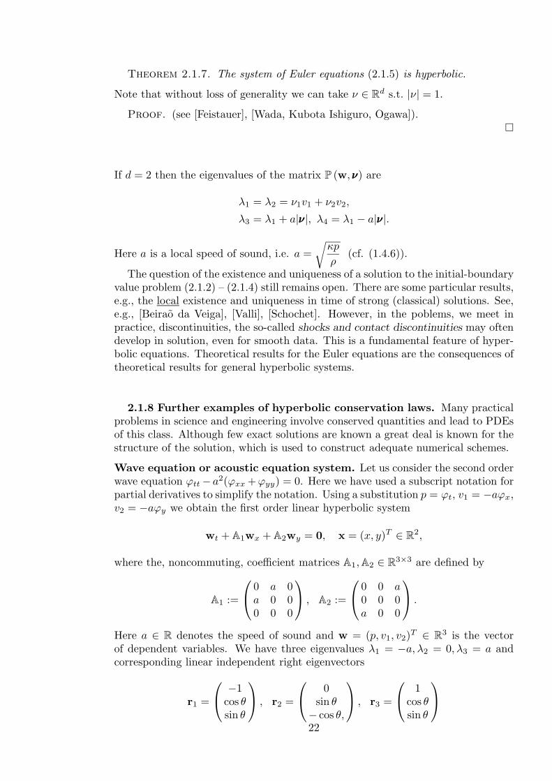
Wave equation or acoustic equation system. Let us consider the second orderwave equation ϕtt − a2(ϕxx +ϕyy) = 0. Here we have used a subscript notation forpartial derivatives to simplify the notation. Using a substitution p = ϕt, v1 = −aϕx,v2 = −aϕy we obtain the first order linear hyperbolic system

wt + A1wx + A2wy = 0, x = (x, y)T ∈ R2,

where the, noncommuting, coefficient matrices A1, A2 ∈ R3×3 are defined by

A1 :=

⎛⎝ 0 a 0

a 0 00 0 0

⎞⎠ , A2 :=

⎛⎝ 0 0 a

0 0 0a 0 0

⎞⎠ .

Here a ∈ R denotes the speed of sound and w = (p, v1, v2)T ∈ R3 is the vectorof dependent variables. We have three eigenvalues λ1 = −a, λ2 = 0, λ3 = a andcorresponding linear independent right eigenvectors

r1 =

⎛⎝ −1

cos θsin θ

⎞⎠ , r2 =

⎛⎝ 0

sin θ− cos θ,

⎞⎠ , r3 =

⎛⎝ 1

cos θsin θ

⎞⎠

22

of the matrix pencil A(ννν) := A1 cos θ + A2 sin θ for any unit vector ννν = (ν1, ν2)T =(cos θ, sin θ)T ∈ R2. Wave equation system is sometimes called the acoustic equa-tion system since it describes propagation of acoustic waves in air. Let us considerlinearized Euler equations written in primitive variables (ρ, v1, v2, p). Here we de-note by u, v the x, y components of the velocity vector, respectively.

ut + B1ux + B2uy = 0, x = (x, y)T ∈ R2,

where the vector of unknowns is

u :=

⎛⎜⎝

ρv1

v2

p

⎞⎟⎠

and the Jacobians frozen at some state (ρ′, v′1, v′2, p

′) are

B1 :=

⎛⎜⎜⎜⎝

v′1 ρ′ 0 0

0 v′1 0

1ρ′

0 0 v′1 0

0 κp′ 0 v′1

⎞⎟⎟⎟⎠ B2 :=

⎛⎜⎜⎜⎝

v′2 0 ρ′ 00 v′

2 0 0

0 0 v′2

1ρ′

0 0 κp′ v′2

⎞⎟⎟⎟⎠ .

Both systems of the Euler equations in primitive and conservative variables areequivalent if ρ, v1, v2, p ∈ C1. Note that it is the wave equation system, whichcreates the key part of the Euler equations. Set ρ′ = 1/a′ and remove the first rowcorresponding to density as well as first column from the Jacobian matrices B1, B2.Then moving the third equation for pressure in the first row leads to the so-calledwave equation system with advection. Further, if the advection velocities are v′

1 =v′2 = 0 and a′ = const. we recover the above linear wave equation system. Thus,

by linearizing the Euler equations about some state (ρ′, v′1, v′2, p

′) we can modelpropagation of sound waves, small disturbances, which propagates with speedsv′1 cos θ+v′

2 sin θ±a′, i.e. with the velocities ±a′ relative to the background velocity(v′

1, v′2). In fact, our ears are sensitive to the small disturbances in pressure in these

waves.Further, the wave equation system describes, for example, propagation of waves

in elastic solids. In exploration seismology one studies the propagation of small am-plitude, man-made waves in the earth, and their reflection off geological structures.The hope is to determine the geological structure from measurements at the surface(for example to order oil reservoirs). Reflection of waves at interfaces can lead todiscontinuities even for linear equations. Earthquakes can cause larger amplitudedisturbances and lead to nonlinear effects.

A similar principle as in seismological exploration of the earth is used for ul-trasound exploration of human tissue. But there are also many other biologicalprocesses involving advection and transport, for example transport of blood cells invessels. As we have said hyperbolic conservation laws can typically produce shockwaves even if the coefficients and data are smooth. Of course, physiologically, atrue shock in arterial circulation is not possible since blood viscosity and elasticityof the vessel wall preclude shock formation. However, it might be possible to gener-ate very steep pressure gradients in the aorta, which are believed to correspond to

23

the pistol-shut phenomenon, a loud cracking sound heard through a stethoscope bypatients with aortic insufficiency. Recently there exists an extensive mathematicalresearch in hemodynamics with the aim to help in prediction of optimal strategyin medical treatment.

Traffic flow. Consider a simple problem of traffic flow on a single-line highway.Let ρ(x, t) denotes the density of cars, 0 ≤ ρ ≤ ρmax, where ρmax is the maximumdensity of cars staying bumper-to-bumper. Cars are moved with the velocity u =U(ρ). There are different models to determine velocity function with respect todensity of cars. The simplest linear model is

U(ρ) = umax

(1 − ρ

ρmax

).

The conservation of cars can be expressed by the following scalar conservation law

∂ρ

∂t+

∂ρu

∂x= 0.

Thus∂ρ

∂t+

∂f(ρ)∂x

= 0,

where f(ρ) = ρumax (1 − ρ/ρmax). Now if one car suddenly stops the cars behindstart to slam into one another and a shock wave will propagate back through theline of cars. Both density as well as velocity of cars jumps across this shock wave.The propagating shock wave is similar to what seen in a gas tube with two differentgases modelled by the Euler equations.

Magnetohydrodynamics. Astrophysical modelling leads to systems of hyper-bolic conservation laws. A spiral galaxy can consist of alternating arms of highdensity and low density, separated by discontinuities, propagating shock waves. Inthis context the shock width may be of order 105 light years. Modelling of dynamicsof a single star, or plasma in a fussion reactor, is governed by the conservation laws.However now also electromagnetic effects together with fluid dynamics have to beconsidered. The magnetohydrodynamic (MHD) equations consist of the Maxwellequation coupled with the Euler equations. In modelling a supernova explosion onemust also include gravitational forces so that density should initially be decreasingwith radius rather than constant and such effects as radiative transfer are impor-tant. Nonetheless, the same basic structure as in simple Riemann problem (shocktube problem) can be found. Note that when gravitational forces directed towardsorigin are included this dense shell will be separated from lighter gas below by acontact surface. In three-dimensional model this surface would initially be sphericalbut would be quickly broken up by the so-called Rayleigh-Taylor instabilities.

Shallow water equations can be found in many practical situations. Forexample, turn on the kitchen faucet full blast and hold a plate or other flat surfaceunderneath. You will see the water rush radially away from the stream in the thinlayer along the plate at fairly high speed. At some distance away from the stream, acircular pattern will generally form, outside of which the layer of water is suddenlythicker and relatively slowly mowing. This discontinuity in depth and velocity iscalled a hydraulic jump, and it is a nice example of a steady shock wave.

24

But there are many other types of flows not necessarily involving water, whichcan be characterized as shallow water flows. They describe flows of fluids with afree surface under the influence of gravity, where the vertical dimension is muchsmaller than any typical horizontal scale. Examples of shallow water are rivers withtheir flood plains, flows in lakes generated by wind blows, propagation of tsunamis,oceanographic, meteorological and geophysical flows.

Sometimes stronger discontinuities can be observed, e.g. tidal bores in some riversor the wave resulting from the bursting of a dam, and a moving step front develops,which is comparable to a shock wave in aerodynamics. In this lecture notes we willconcentrate on problems involving bores or hydraulic jumps and therefore the aimis to use such numerical schemes which take into account the hyperbolic characterof the equations and allow modelling of discontinuous flows.

For example, typical lengths of the river Rhine are: length 1000 km, width 100m,depth 5m. As we see there is just one dominant scale and thus one-dimensionalequations will be a good model for the river flow. In what follows we derive theone-dimensional shallow water equations.

Let us consider a fluid which is incompressible, non-viscous, non-heat conducting,and neglect the vertical velocity as well as dependency on vertical direction due tothe shallow effects. Since the fluid is incompressible the density ρ is constant. Butthe height h(x, t) of the shallow water may vary. Let η(x, t) describes the free watersurface and b(x) relief of bottom solid surface. Thus h(x, t) = η(x, t) − b(x), andthe total mass in some volume σ(t) = [x1(t), x2(t)]× cross-sectional area at time tis

m(σ(t)) =∫ x2(t)

x1(t)

ρh(x, t)dx.

The conservation of mass postulates that∂m(σ(t))

∂t= 0. Using the Transport the-

orem 1.1.1 and the fact that ρ = const. we get

(i) ht + (hu)x = 0,

where u(x, t) denotes the velocity of the shallow water. Further, the one-dimen-sional momentum equation (1.2.2’) with zero outer forces yields

(ii) ut + uux = −1ρpx.

Now the pressure p is determined from a hydrostatic law, stating that the pressureat the depth y is ρg(η − y), where g is the gravitational constant. Thus,

(iii) px = ρgηx.

We multiply equation (i) by u and equation (ii) by h. Adding them together andusing (iii) yields the momentum equation for the one-dimensional shallow water inconservative variables

(iv) (hu)t + (hu2 +12gh2)x = −ghbx.

Equations (i) and (iv) form the one-dimensional shallow water system.25

In more general situations, e.g. oceanography or meteorology, full three-dimen-sional flows have to be considered. Under the assumption on shallow effects theycan be modelled mathematically by the two-dimensional shallow water equationswith a source term

∂w∂t

+∂f(w)

∂x+

∂g(w)∂y

= t(w), x = (x, y)T ∈ R2,

where

w =

⎛⎝ h

huhv

⎞⎠ f(w) =

⎛⎝ hu

hu2 + gh2

2huv

⎞⎠ ,

g(w) =

⎛⎝ hv

huvhv2 + gh2

2

⎞⎠ , t(w) =

⎛⎝ 0

−gh ∂b∂x + fhv − ghSf1

−gh ∂b∂y − fhu − ghSf2

⎞⎠ .

Here u, v are the x, y components of the depth averaged velocities of the flow,respectively. In general, there are more then just the bottom relief effects. Forexample, the Coriolis forces f arise from earth’s rotation and Sf1, Sf2 are fric-tion slopes resulting from viscosity effects. Due to the bottom friction terms theflow is retarded. Usually it is assumed that the bottom friction stresses dependquadratically on the depth-averaged velocities.

The eigenvalues of this hyperbolic conservation law are λ1 = u cos θ + v sin θ −√gh, λ2 = u cos θ + v sin θ, λ3 = u cos θ + v sin θ +

√gh, where θ ∈ [0, 2π) and√

gh = c denotes the wave celerity or the wave speed. The corresponding linearlyindependent right eigenvectors are

r1 =

⎛⎝ 1

u − c cos θv − c sin θ

⎞⎠ , r2 =

⎛⎝ 0

sin θ− cos θ

⎞⎠ , r3 =

⎛⎝ 1

u + c cos θv + c sin θ

⎞⎠ .

Analogously as in the gas dynamics we introduce the so-called Froude number

Fr =|v|c

,

which plays an important role in the classification of shallow flows. The shallowflow is called supercritical, critical or subcritical for Fr > 1, Fr = 1, and Fr < 1,respectively.

Exercise:Derive the two-dimensional shallow water equations in primitive variables (h, u, v).Which are the regularity conditions you need to assume? Compute the eigenvaluesand the corresponding eigenvectors! Explain why the eigenvalues did not change!

2.1.9 Hyperbolic systems. In this subsection the theory of multi-dimensionalhyperbolic conservation laws will be reviewed. The theory gives a good insight intounderlying properties that occur in an analytical solution of a set of conservationlaws. The aim is to get a better understanding of properties of solutions to hyper-bolic systems such that they can be used in construction of an adequate numerical

26

scheme. To simplify the situation we will consider the Cauchy problem (we elimi-nate boundary conditions):

(2.1.10)∂w∂t

+d∑

j=1

∂

∂xjfj (w) = 0 in R

d × 〈0,∞),

(2.1.11) w (·, 0) = w0 in Rd,

where w : Rd×〈0,∞) → D, D ⊆ Rs is an open set, fj ∈ C1 (D; Rs) , j = 1, 2, . . . , d.Here s states for the number of equations and d is a dimension.

Repeating Definition 2.1.6 for general case of vector w and fj , j = 1, 2, . . . , d,we get the definition of hyperbolic systems. In what follows we assume that thesystem (2.1.10) is hyperbolic. The concept hyperbolic conservation laws is also usedin literature. By the definition of hyperbolic system the equivalent form of (2.1.10)is

(2.1.12)∂w∂t

+d∑

j=1

Aj (w)∂w∂xj

= 0,

where Aj (w) =Dfj (w)

Dw, and the matrix P (w, ννν) =

d∑j=1

νjAj (w) ; w ∈ D, ννν ∈ Rd;

has s real eigenvalues λi = λi (w, ννν) , i = 1, 2, . . . , s.

Definition 2.1.13. A vector valued function w ∈ C1(Rd × 〈0,∞);D

)satisfy-

ing (2.1.10), (2.1.11) pointwise is called a classical solution.

We have already mentioned that an important property of hyperbolic conserva-tion law is that it may develop discontinuities in the solution, even if the data w0

and fj are infinitely smooth. This can be shown even for very simple example ofthe Cauchy problem for inviscid Burgers’ equation (d = s = 1) :

(2.1.14)∂u

∂t+

∂

∂x

(u2

2

)= 0,

u (x, 0) =

⎧⎪⎨⎪⎩

1, x ≤ 0,

1 − x, 0 ≤ x ≤ 1,

0, 1 ≤ x.

The solution of the first order parabolic equation (2.1.14) can be found by themethod of characteristics. The characteristics x = x (t) of (2.1.14) satisfy

(2.1.15)d

dtx (t) = u (x (t) , t) ,

and along each characteristic u is constant, since

d

dtu (x (t) , t) =

∂

∂tu (x (t) , t) +

∂

∂xu (x (t) , t) · d

dtx (t) =

∂u

∂t+ u

∂u

∂x= 0.

27

t

x0

1

1

Fig. 2.1. Characteristics for the Burgers equation (2.1.14).

Moreover, since u is constant on each characteristic, the sloped

dtx (t) is constant

by (2.1.15) . Thus, the characteristics are straight lines, determined by the initialdata (see Fig. 2.1).

The characteristics do not intersect for t < 1 and the solution, constant alongcharacteristics, is

(2.1.16) u (x, t) =

⎧⎪⎨⎪⎩

1, x ≤ t,

(1 − x)/(1 − t), t ≤ x ≤ 1,

0, x ≥ 1,

for t < 1.

At the point (1, 1) the characteristics intersect and the discontinuity of the solutiondevelops. It will be shown that for t ≥ 1 a generalized weak solution with thediscontinuity on the line x = (t + 1) /2 can be defined in the form

(2.1.16′) u (x, t) =

⎧⎪⎨⎪⎩

1, x <t + 1

2,

0, x >t + 1

2,

for t ≥ 1.

A very suitable technique to describe such phenomena is the theory of distri-butions. Thus, in order to admit also discontinuous solutions one has to use theweak formulation of conservation laws. This notation is analogous to the conceptof weak solution already defined in previous courses of partial differential equa-tions. Note however, that because of less regularity, i.e. “smoothness”, of solutionsto hyperbolic problems, the Sobolev spaces W k,l used for parabolic and ellipticequations are inappropriate in our case. The only thing we can assume aboutthe solution is that it does not blow up, i.e. it is “essentially” bounded. Thus,we need to work with the class L∞

loc of locally bounded measurable functions, i.e.L∞

loc

(Rd

)≡

{w; ‖w‖L∞(K) < ∞ ∀K ⊂ Rd, K compact

}. See also [Kroner], [Feis-

tauer] for more details.

Definition 2.1.17. Let C∞0

(Rd × 〈0,∞); Rs

):=

{ϕϕϕ ∈ C∞ (

Rd × 〈0,∞); Rs);

supp ϕϕϕ is a compact set in Rd × 〈0,∞)}

and w0 ∈ L∞loc

(Rd;D

). A vector valued

28

function w, s.t. w ∈ L∞loc

(Rd × 〈0,∞);D

), is called a weak solution to the problem

(2.1.10), (2.1.11), if the following integral identity holds

∫ ∞

0

∫Rd

⎛⎝w

∂ϕϕϕ

∂t+

d∑j=1

fj (w)∂ϕϕϕ

∂xj

⎞⎠

(2.1.18)

+∫

Rd

w0 ϕϕϕ (·, 0) = 0 ∀ϕϕϕ ∈ C∞0

(R

d × 〈0,∞); Rs).

Exercise:

Show that the classical solution (2.1.13) is a weak one, and conversely: a weaksolution satisfies (2.1.10) , (2.1.11) in the sense of distributions on Rd × (0,∞).

Further, it follows from the weak formulation that across discontinuities theso-called Rankine–Hugoniot relation must hold.

Definition 2.1.19. A function w : Rd × 〈0,∞) → Rs is piecewise smooth ifthere is a finite number of smooth hypersurfaces Γ in Rd × 〈0,∞) s.t. the functionw is smooth in Rd ×〈0,∞) \Γ and has one-sided limits w± on Γ, i.e. w± (x, t) :=lim

ε→0+w ((x, t) ± εn) , where n = (nx1 , nx2 , . . . , nxd

, nt) is a normal to Γ.

Theorem 2.1.20. (Rankine–Hugoniot condition) Let w : Rd×〈0,∞) → D ⊂ Rs

be a piecewise smooth function. Then w is a solution of (2.1.10) in the sense ofdistributions on Rd × (0,∞) if and only if it satisfies the following conditions :

(1) w is a classical solution in any domain where w is C1 function;(2) jump condition: (w+ − w−) nt +

∑dj=1

(fj (w+)− fj (w−)

)nj = 0 on any

hypersurface of discontinuity Γ.

Proof. Do it as an exercise!�

Let us come back to the example (2.1.14). We can verify that the Rankine–

Hugoniot condition (2.1.20)ii) holds on Γ ={

(x, t) ; x =t + 1

2, t > 1

}. The outer

normal to the hypersurface of discontinuity Γ = {(x, t) ; x = ξ (t)} can be expressed

in the form n = (nx, nt) = (1,−s), where s =dξ (t)

dt. The Rankine–Hugoniot

condition becomes

(2.1.21) s(u+ − u−)

= f(u+

)− f

(u−)

.

From (2.1.16) we get that u+ − u− = 1, f (u+) − f (u−) = 12 at (x, t) = (1, 1) .

Since, by the definition of Γ, s = 12 , the condition (2.1.21) is satisfied.

It is easy to verify that outside Γ the function u, define in (2.1.16′), is a classicalsolution. Thus, it is a weak solution on R × 〈0,∞).

29

Unfortunately, there is often more than one weak solution to the conservationlaw with the same initial data. For example, if we solve Burgers’ equation (2.1.14)with the initial data

(2.1.22) u (x, 0) =

⎧⎨⎩

0, x ≤ 0,

1, x > 0,

then there are infinitely many weak solutions. For example,

(2.1.23) u (x, t) =

⎧⎪⎪⎪⎪⎨⎪⎪⎪⎪⎩

0, x < smt,

um, smt ≤ x ≤ umt,x

t, umt ≤ x ≤ t,

1, x > t;

is a weak solution for any um s.t. 0 ≤ um ≤ 1 and sm =um

2. This can be easily

verified by Theorem 2.1.20.If our conservation law is to model the real world then clearly only one of the

solutions is physically relevant. The fact, that the equations have other, spurious,solutions is a result of the fact that our equations are only a model of reality andsome physical effects have been ignored. In particular, hyperbolic conservation lawsdo not include diffusive or viscous effects. Although these effects may be negligiblethroughout most of the flow, near discontinuities the effect is always strong. In fact,the full Navier–Stokes equations have smooth solutions, for some simple problemsthat we consider, and the apparent discontinuities are in reality thin regions. Whatwe hope to model with the Euler equations is the limit of the smooth solution tothe Navier–Stokes equations as the viscosity parameter approaches zero. This leadsto the desired weak solution of the Euler equations.

But there are also other weak solutions even to simple hyperbolic conservationequations. We must use our knowledge of what is being ignored. This helps to pickout the correct weak solution.

The following approach, called vanishing viscosity method, was suggested byP. D. Lax in 1954. We introduce a missing diffusive term into the equation andobtain an equation with a unique smooth solution. Then let the coefficient of thisterm tends to zero. This idea of vanishing viscosity method is used in analysisof conservation laws and very often for the construction of sufficiently dissipativenumerical scheme, which gives physically relevant approximate solutions.

On the other hand, this method is not optimal in order to define physicallyrelevant solution, since it requires study of a more complicated system of equations.This is precisely what we wanted to avoid by introducing an inviscid fluid. But itis a good hint in order to derive other condition that can be imposed directlyon the weak solutions of the hyperbolic system to pick out the physically correctsolution (cf. Theorem 2.1.27). Taking into account the physical background we see asuitable candidate for such a condition, namely the second law of thermodynamics(cf. (1.3.11)) or the entropy condition. It says that entropy is nondecreasing intime. In fact, as molecules of a gas pass through a shock their entropy increase.Now we approach the mathematical definition of entropy.

30

Definition 2.1.24. A convex function U : Rs → R is said to be entropy of(2.1.10), if there are some entropy fluxesF1, . . . , Fd : D ⊂ Rs → R, s.t.

(2.1.25)(grad U (w)

)T · Dfj (w)Dw

= grad Fj (w) , j = 1, 2, . . . , d.

It can be verified easily that the entropy U (w) is conserved for smooth solutionsof hyperbolic conservation laws (2.1.10), thus

(2.1.26)∂U (w)

∂t+

d∑j=1

∂Fj (w)∂xj

= 0

holds in the sense of distributions on Rd × (0,∞).But for the discontinuous solutions we cannot perform the same manipulations.

Since we are particularly interested in how the entropy behaves for the vanishingviscosity weak solution, we look at the related viscous problem and then let theviscosity tend to zero. This is exactly what the following theorem says.

Theorem 2.1.27. Let system (2.1.10) have a convex entropy U ∈ C2 (Rs; R)and entropy fluxes Fj ∈ C1 (Rs, R) , j = 1, 2, . . . , d. Let {wε} be a sequence ofsufficiently smooth solutions to the pertubated Cauchy problem (2.1.10) , (2.1.11),i.e. the R.H.S. of (2.1.10) is equal to εΔwε. Let the following conditions hold

(i) ‖wε‖L∞

(Rd×(0,∞);Rs

) ≤ c,

uniformly with respect to ε > 0,

(ii) wε → w as ε → 0 a.e. in Rd × 〈0,∞).

Then w is a weak solution of (2.1.10) , (2.1.11) and

(2.1.28)∂U (w)

∂t+

d∑j=1

∂

∂xjFj (w) ≤ 0

holds in the sense of distributions on Rd × (0,∞), i.e.

(2.1.29)∫ ∞

0

∫Rd

U (w)∂ϕ

∂t+

d∑j=1

Fj (w)∂ϕ

∂xj≥ 0

for all ϕ ∈ C∞0

(Rd × (0,∞)

), ϕ ≥ 0.

Proof. (see, e.g., [Kroner]).�

Now we define an entropy solution on the basis of the result from Theorem 2.1.27.31

Definition 2.1.30. A weak solution w, s.t. w ∈ L∞loc

(Rd × 〈0,∞); Rs

), of the

Cauchy problem (2.1.10) , (2.1.11), is said to be an entropy weak solution, if for allentropies U and corresponding entropy fluxes Fj , j = 1, 2, . . . , d,

∂U (w)∂t

+d∑

j=1

∂

∂xjFj (w) ≤ 0

holds in the sense of distributions on Rd × (0,∞).

A natural suggestion arises : what is a relation between the mathematical entropyU and the physical entropy η (cf. (1.3.10))? In reference [Feistauer], it was shownthat for the Euler equations this relation is

(2.1.31) U = −ρ η, Fj = −ρ vj η, j = 1, 2, . . . , d.

The inequality (2.1.28) becomes

(2.1.32)∂

∂t(ρ η) +

d∑j=1

∂

∂xj(ρ vj η) ≥ 0

in the sense of distributions on Rd×(0,∞). Hence, using (2.1.32) and the continuityequation (1.1.3) we obtain

(2.1.33) ρd

dt(η) ≥ 0 (in the sense of distributions) .

This inequality is in agreement with the second law of thermodynamics (1.3.11),where now q = 0, q = 0. Thus, (2.1.33) is the mathematical formulation of thewell-known fact: entropy of the system is not decreasing in time.

Although there is still hope that there exists the weak entropy solution even inthe case of a general hyperbolic system and consequently, of the Euler equations,too, till now it has not been proved. As far as the uniqueness concerns, thereis a counter example to the uniqueness of entropy solution to a hyperbolic system[Sever]. Nevertheless, it is still believed that there is a unique weak entropy solutionof the Euler equations. In the scalar case (s = 1) we have a fundamental Kruzhkov’sresult, which holds in any space dimension d.

Theorem 2.1.34. (Kruzhkov, 1970) If w0 ∈ L∞ (Rd

), then the problem (2.1.10)

(2.1.11), where s = 1, has a unique weak entropy solution w ∈ L∞ (Rd × 〈0,∞)

).

Proof. (see [Kruzhkov]).�

Remark 2.1.35. This Kruzhkov solution can be found by the method of van-ishing viscosity. By adding a term εΔwε to the R.H.S. of (2.1.10), we get theparabolic perturbation of (2.1.10), i.e.

∂wε

∂t+

d∑j=1

∂

∂xjfj (wε) = εΔwε in R

d × (0,∞) ,

wε (·, 0) = w0 in Rd, ε > 0.

32

The aim is to study the behaviour of the solution wε when passing to the limitas ε → 0. We will not go into the details of the proof, we just note that onepossible approach is based on the concept of the measure-valued solution , whichis a solution taken even in a weaker sense than the concept of the weak solutions.This concept is often used to study the convergence of numerical methods used forapproximation of hyperbolic conservation laws; as an example see Theorem 2.2.52.

In the case of general hyperbolic systems of first order there are only particularexistence and uniqueness results for the one-dimensional situation. For the restof this section we assume that d = 1 and s ≥ 1. The existence of weak entropysolution was proved by Glimm in 1965. In order to formulate this result we needto introduce some new concepts.

Definition 2.1.36. Let w ∈ L1loc(R). The total variation of w is given as

TV (w) ≡ suph∈R−{0}1h

∫R

|w(x + h) − w(x)| dx.

The space of all functions from R to Rs with bounded total variation is defined as

BV (R) ≡ {w ∈ L1loc(R);TV (w) < ∞},

and the associated norm is given in the following way

‖w‖BV ≡ ‖w‖L1 + TV (w).

For simplification we are using here and in what follows notations L1loc(R), BV (R)

instead of more precise L1loc(R; Rs), BV (R; Rs), respectively. From the definition

above it follows how to understand total variation of sequences approximating dis-crete functions. Let w = {wj}j∈N be a sequence of discrete values wj . Then wehave for the total variation of w

TV (w) =∞∑

j=0

|wj+1 − wj |.

In order to get better understanding of how large the BV space is, let us recalla powerful compactness property, the well-known selection principle of Helly.

Theorem 2.1.37. (Selection principle of Helly) Let {un} be a sequence of func-tions in L1(a, b) such that

‖un‖L∞[a,b] ≤ c, TV[a,b](un) ≤ c n ∈ N.

Then there exists a subsequence {un′} and an u ∈ L1(a, b) such that

un′ −→ u in L1(a, b).

�In fact, we have for the BV spaces the following imbedding properties W 1,1

loc (R) ↪→BV (R) ↪→↪→ L1

loc(R).

Let rk (w) , k = 1, 2, . . . , s, be the eigenvectors of the Jacobian matrix A (w) ,w ∈D, and λk (w) , k = 1, 2, . . . , s, be the corresponding eigenvalues, cf. (2.1.12).

33

Definition 2.1.38. An eigenvector rk is called genuinely nonlinear, if

grad λk (w) · rk (w) �= 0 ∀w ∈ D.

We say that rk is linearly degenerate, if

grad λk (w) · rk (w) = 0 ∀w ∈ D.

Now we can approach to the formulation of the existence result of Glimm.

Theorem 2.1.39. (Glimm, 1965) Let the initial data w0 ∈ L∞loc(R) and let there

exist δ > 0, such that the total variation TV (w0) < δ. Further, let the system bestrictly hyperbolic, i.e. all eigenvalues λk(w) are distinct, and let each eigenvector iseither genuinely nonlinear or linearly degenerate. Then there exists a weak entropysolution w ∈ L∞ ([0, T ], BV (R) ∩ L∞

loc(R)) of (2.1.10), (2.1.11), (d = 1).

In 1995 Bressan, see e.g. [Bressan], proved the uniqueness of the weak en-tropy solution in the above class of BV solutions using the semigroup technique.Let us note that the assumption on small total variation is necessary; namely ifTV (w0) → ∞ there exist at least two weak entropy solutions to the system (2.1.10),(2.1.11), (d = 1).

2.1.40 Riemann problem. Many of nowadays numerical schemes used forhyperbolic systems, cf. Godunov finite volume methods 2.2.54, are based on findinga solution, or at least its approximation, to the Riemann problems solved in thenormal directions to the mesh cell interfaces. We will deal with this point moredeeply in the next Section 2.2, where the finite volume methods are described. Theaim of this section is to show properties of solution of the following one-dimensionalRiemann problem

∂w∂t

+ A (w)∂w∂x

= 0 on R × (0,∞) ,(2.1.41)

w (x, 0) =

⎧⎨⎩

wL, x < 0,

wR, x > 0

with given constant initial states wL, wR ∈ D. As a physical interpretation of(2.1.41) we can imagine a long tube filled with two types of gas, e.g. rare and densegas. These are separated with a membrane. We are interested in the gas motionafter the membrane is suddenly removed. In Fig. 2.2 solution of the Riemannproblem for the Euler equations is plotted. Initial data are taken as follows:

ρ = 1, p = 1, v1 = v2 = 0 x ≤ 0ρ = 0.125, p = 0.1, v1 = v2 = 0 x > 0.

We can notice all three fundamental parts of solution: rarefaction wave, contactdiscontinuity and shock, which we will describe in what follows.

Theorem 2.1.42. (Self-similarity form) Let the Riemann problem (2.1.41) hasa unique piecewise smooth weak solution w, then w can be written in the similarityform w(x, t) = w(x/t), where w : R → Rs, t > 0.

34

0.2 0.4 0.6 0.80

0.5

1

1.5

2

2.5

3

3.5Density at time t = 0.25

0.2 0.4 0.6 0.8−0.5

0

0.5Velocity at time t = 0.25

0.2 0.4 0.6 0.80

0.5

1

1.5

2

2.5

3

3.5Pressure at time t = 0.25

0.2 0.4 0.6 0.80

0.5

1

1.5

2Temperature at time t = 0.25

Fig. 2.2. Solution to the Riemann problem of the Euler equations;plots of density, velocity, pressure and temperature at t = 0.25.

Proof. It is easy to realize that w(αx, αt) is also a solution of (2.1.41) for everyα > 0. Due to the uniqueness, we have w(αx, αt) = w(x, t), which means that w ishomogeneous of order zero. Now, taking α = 1/t, we see that w(x, t) = w(x/t, 1) =w(x/t).

�

Solution to the linear Riemann problem. Assume that in (2.1.41) the Jacobianmatrix A = const. The system {rk}s

k=1 of all eigenvectors of A creates a basis inRs. Thus,

wL :=s∑

k=1

αkrk, wR :=s∑

k=1

βkrk,

and we can rewrite the initial data by means of

w0 =s∑

k=1

[H(x)βk + (1 − H(x))αk] rk.

Here H(x) denotes the Heaviside function, i.e. H(x) = 1 for x ≥ 0 and H(x) = 0else. Let T−1 denotes the inverse matrix to the matrix T consisting of all eigenvec-tors rk. Further denote by u the characteristic vector, i.e.

u = T−1w.

Multiplying system (2.1.41) by the matrix T−1 from the left leads to the diagonalsystem

∂u∂t

+ D∂u∂x

= 0 on R × (0,∞) ,(2.1.42)35

with D = T−1AT. This system consists of s separated linear advection equationsfor each component k. Thus, analogously we can write

∂uk

∂t+ λk

∂uk

∂x= 0, k = 1, . . . , s,

and accompany them with the initial data

uk(x, 0) ={

αk x < 0,

βk x ≥ 0.

Now similarly as for advection equation (2.1.14) each component uk is deter-mined by the initial data backwards along the characteristic dx/dt = λk. Thus,

(2.1.43) uk(x, t) = uk(x − λkt, 0), k = 1, . . . , s.

Multiplying (2.1.43) by rk and summing over each k = 1, . . . , s, we obtain

w(x, t) =s∑

k=1

uk(x, t) rk =s∑

k=1

uk(x − λkt, 0) rk

s∑k=1

[βkH(x − λkt) + αk(1 − H(x − λkt))] rk.(2.1.44)

If −∞ = λ0 < λ1 ≤ λ2 ≤ · · · ≤ λs < λs+1 = ∞ and for some k ≥ 0 λk < λk+1

then w is constant in the domain Ωk = {(x, t); t > 0, λk < x/t < λk+1}:

w(x, t) = wk (x, t) ∈ Ωk,

wk =k∑

j=1

βjrj +s∑

j=k+1

αjrj , k = 1, . . . , s.

Exercise:Show that the function w defined in (2.1.44) is a weak solution to the linear Riemannproblem (2.1.41).Hint : Use Theorem 2.1.20 and show that on each discontinuity x/t = λk theRankine-Hugoniot conditions are satisfied.

Solution to the nonlinear Riemann problem. Above we have shown thatsolution to the linear Riemann problem consists of constant states, sometimes calledwaves, separated by discontinuities x/t = λk, which are also called linear shocks.In what follows we will deal with nonlinear problem (2.1.41). We will see that thestructure of solution will be now more complex. First we have to introduce somenew concepts.

I. Shock discontinuity. Let the k-th eigenvector rk, k = 1, . . . , s, be genuinely non-linear, cf. Definition 2.1.38. Let w be a piecewise discontinuous solution to (2.1.41),such that

(2.1.45) w(x/t) ={

wL x/t < λ

wR x/t > λ,36

where λ denotes the speed of propagation of discontinuity (direction of discontinu-ity) corresponding to the eigenvector rk. The weak entropy solution in the formof (2.1.45) have to satisfy the Rankine-Hugoniot conditions, cf. Theorem 2.1.20, aswell as the entropy condition, cf. Definition 2.1.30.Due to the Rankine-Hugoniot conditions

(2.1.46) f(wL) − f(wR) = λ(wL − wR).

Moreover we assume that the following so-called Lax entropy condition is satisfied

(2.1.47) λk(wL) > λ > λk(wR).

It was proved by Lax [Lax (1)] that for one-dimensional systems condition (2.1.47)is for genuinely nonlinear eigenvectors equivalent to the entropy inequality (2.1.29).

If conditions (2.1.46), (2.1.47) hold, solution (2.1.45) is called shock discontinuityor shock.

II. Rarefaction wave. Assume again that the k-th eigenvector rk, k = 1, . . . , s, isgenuinely nonlinear. Now let w be a continuous solution to (2.1.41), constructed insuch a way that the gap between λk(wL) and λk(wR), λk(wL) < λk(wR), is filledwith a fan

(2.1.48) λk(w(x/t)) =

⎧⎪⎨⎪⎩

λk(wL), x/t < λk(wL)x/t, λk(wL) < x/t < λk(wR)λk(wR), x/t > λk(wR).

Now, a piecewise smooth weak solution of the Riemann problem (2.1.41) satis-fying (2.1.48) can be written in the following form

(2.1.49) w(x, t) =

⎧⎪⎨⎪⎩

wL, x/t < λk(wL)w(x/t), λk(wL) < x/t < λk(wR)wR, x/t > λk(wR)

with C1- smooth function w. The weak solution given by (2.1.49) is called a weakrarefaction wave or a simple wave. Note, that since w is C1-smooth function theentropy condition is fulfilled as equality (2.1.26).

III. Contact discontinuity. Now, let us assume that the k-th eigenvector rk is lin-early degenerate, cf. Definition 2.1.38. We look for a piecewise discontinuous solu-tion w to (2.1.41) in the form (2.1.45). Since w is a weak solution, the Rankine-Hugoniot conditions (2.1.46) have to be satisfied on the discontinuity x/t = λ.Further,

(2.1.50) λk(wL) = λ(wR) ≡ λ,

which follows from the definition of contact discontinuity. Namely,

λk(w(ξ))dξ

= grad λk(w(ξ)) · rk(w(ξ)) = 0.

37

The weak entropy solution (2.1.45), which corresponds to the linearly degenerateeigenvector rk, is called a contact discontinuity or a slip contact. Note, that thisweak discontinuous solution is also an entropy one. It follows from the fact that k-th eigenvalue λk stays constant, and thus the problem has in the k-th characteristicfield linear-like behaviour, see [Feistauer] for a precise proof.

Now we can approach to the formulation of the existence and uniqueness result forthe solution of nonlinear Riemann problem. We present this result without a proof,the reader can find more details e.g. in [Lax (2)].

Theorem 2.1.51. (Lax solution to the Riemann problem) Let the hyperbolic sys-tem in (2.1.41) be strictly hyperbolic and each eigenvector be either genuinely non-linear or linearly degenerate. Let for the initial conditions of the Riemann problem(2.1.41) the difference |wR−wL| be “sufficiently small”. Then there exists a uniqueweak entropy solution to (2.1.41), which consists of at most s + 1 constant statesseparated either by rarefaction waves or shock waves or contact discontinuities.

Remark 2.1.52. Let us note that the above general considerations for theRiemann problem can be used for particular systems used in practical applications;e.g. the shallow water equations, the Euler equations. For example, for the x-splittwo-dimensional shallow water equations the vectors w and f(w) are

w =

⎛⎝ h

huhv

⎞⎠ , f(w) =

⎛⎝ hu

hu2 + 12gh2

huv

⎞⎠ .

We have three wave families, which are associated with the eigenvalues λ1 = u −a, λ2 = u, λ3 = u + a; a =

√gh. These three waves separate four constant states

wL,wR, which are the left and right given data, and w∗L,w∗

R, which are the leftand right intermediate states to be determined.

The left and right waves are shocks or rarefactions, while the middle wave isalways a shear wave, i.e. the contact discontinuity wave. Across the left and rightwaves both h and u change, but v remains constant. The tangential velocity vchanges across the shear wave discontinuously, other components h and u are con-stant here. As a result we have for the intermediate star region

w∗L =

⎛⎝ h∗

h∗u∗

h∗vL

⎞⎠ , w∗

R =

⎛⎝ h∗

h∗u∗

h∗vR

⎞⎠ .

The following conditions determine the type of the waves which occur:h∗ > hL . . . left wave is a shockh∗ ≤ hL . . . left wave is a rarefaction wave;h∗ > hR . . . right wave is a shockh∗ ≤ hR . . . right wave is a rarefaction wave.

The basic step is to derive two non-linear algebraic equations, which determine h∗

and u∗. This follows from the so-called generalised Riemann invariants, which arethe ordinary differential equations holding across the corresponding waves, cf., e.g.,

38

[Toro] for details. In fact for the Riemann problems arising in most practical appli-cations, we can compute exact solution to the one-dimensional Riemann problem.However, due to nonlinearity of the algebraic equations, h∗ and u∗ are actuallycomputed by some suitable iterative methods, e.g. Newton’s iterations.

Remark 2.1.53. In the case of two-dimensional Riemann problem the initialdata consists of arbitrary many constant states prescribed in sectors around theorigin (0, 0). Note that the question of existence and uniqueness of the weak entropysolution to the two-dimensional Riemann problem for nonlinear systems is an openproblem. Some particular results have been proven either for linear systems orsimplified nonlinear systems, see e.g. Li et al. [Li, Zhang, Yang], [Li, Lukacova,Warnecke].

In Figure 2.3 the two-dimensional circular analogy of the above one-dimensionalRiemann problem is modelled by a genuinely multidimensional finite volume me-thod, the so-called evolution Galerkin method, cf. [Lukacova, Morton, Warnecke],[Lukacova, Saibertova, Warnecke]. The initial data of the so-called two-dimensionalSod problem are given as

ρ = 1, u = 0, v = 0, p = 1, ‖x‖ < 0.4ρ = 0.125, u = 0, v = 0, p = 0.1, else.

Figure 2.3 shows the isolines of density, x−, y− velocity components and pres-sure computed at time T = 0.2 by the second order finite volume evolution Galerkinscheme. The solution exhibits analogous phenomena as in the one-dimensional case.Namely, a circular shock travelling away from the center, a circular contact discon-tinuity travelling in the same direction and a circular rarefaction wave travellingtowards the origin at (0, 0).

2.2 Finite Volume Method

In this section we derive commonly used numerical scheme for solving the Eulerequations, the so-called finite volume methods (FVM). Generally, one has threebasic numerical methods for solving PDE’s. Namely, the finite difference method,the finite element method and the finite volume method. Advantages of the FVMare the simplicity of the scheme and the automatic control of the conservation,which is a crucial property.

Let us present a derivation of the FVM on the following two-dimensional (i.e.d = 2) initial-boundary value problem

∂w∂t

+d∑

k=1

∂ fk (w)∂xk

= 0 in QT ≡ Ω × (0, T ),(2.2.1)

w (·, 0) = w0 in Ω,(2.2.2)

B (w) = b on ∂Ω × (0, T ) ,(2.2.3)39

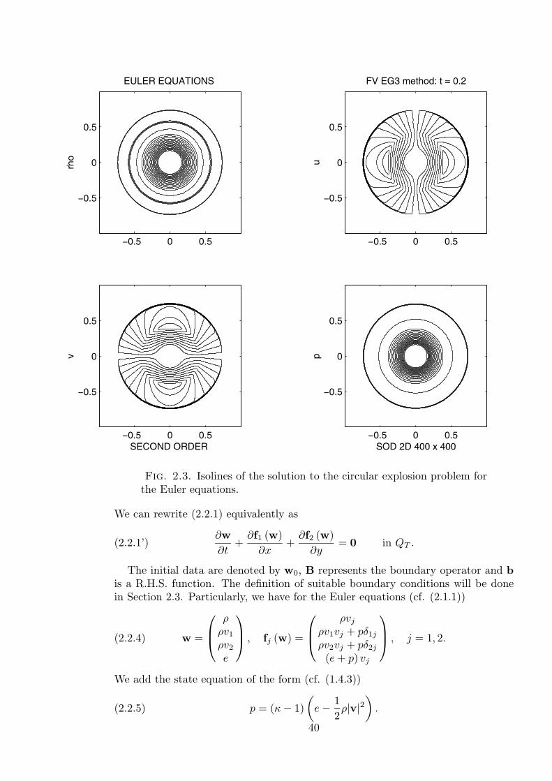
−0.5 0 0.5

−0.5

0

0.5

EULER EQUATIONS rh

o

−0.5 0 0.5

−0.5

0

0.5

FV EG3 method: t = 0.2

u

−0.5 0 0.5

−0.5

0

0.5

SECOND ORDER

v

−0.5 0 0.5

−0.5

0

0.5

SOD 2D 400 x 400

p

Fig. 2.3. Isolines of the solution to the circular explosion problem forthe Euler equations.

We can rewrite (2.2.1) equivalently as

(2.2.1’)∂w∂t

+∂f1 (w)

∂x+

∂f2 (w)∂y

= 0 in QT .

The initial data are denoted by w0, B represents the boundary operator and bis a R.H.S. function. The definition of suitable boundary conditions will be donein Section 2.3. Particularly, we have for the Euler equations (cf. (2.1.1))

(2.2.4) w =

⎛⎜⎝

ρρv1

ρv2

e

⎞⎟⎠ , fj (w) =

⎛⎜⎝

ρvj

ρv1vj + pδ1j

ρv2vj + pδ2j

(e + p) vj

⎞⎟⎠ , j = 1, 2.

We add the state equation of the form (cf. (1.4.3))

(2.2.5) p = (κ − 1)(

e − 12ρ|v|2

).

40

Let Aj (w) =Dfj (w)

Dw, j = 1, 2, w ∈ D ⊂ R4, be the Jacobian matrices. It can

be shown that

A1 =(2.2.6)

⎛⎜⎜⎜⎜⎝

0 1 0 0κ − 3

2v21 +

κ − 12

v22 (3 − κ) v1 (1 − κ) v2 κ − 1

−v1v2 v2 v1 0

−κev1

ρ+ (κ − 1) v1|v|2

κe

ρ− κ − 1

2(3v2

1 + v22

)(1 − κ) v1v2 κv1

⎞⎟⎟⎟⎟⎠

A2 =(2.2.7)

⎛⎜⎜⎜⎜⎝

0 0 1 0−v1v2 v2 v1 0

κ − 32

v22 +

κ − 12

v21 (1 − κ) v1 (3 − κ) v2 (κ − 1)

−κev2

ρ+ (κ − 1) v2|v|2 (1 − κ) v1v2

κe

ρ− κ − 1

2(3v2

2 + v21

)κv2

⎞⎟⎟⎟⎟⎠

Due to hyperbolicity of the Euler equations the matrix

(2.2.8) P (w, ννν) = ν1A1 (w) + ν2A2 (w) ,

where w ∈ D, ννν ∈ R2, is diagonalizable, i.e.

(2.2.9) P = T · D · T−1,

T = T (w, ννν) is a nonsingular matrix

T =

⎛⎜⎝

1 0 1/(2a2) 1/(2a2)v1 n2 (v1 + an1)/(2a2) (v1 − an1)/(2a2)v2 −n1 (v2 + an2)/(2a2) (v2 − an2)/(2a2)

|v|2/2 n2v1 − n1v2 (H + av · n)/(2a2) (H − av · n)/(2a2)

⎞⎟⎠ ,

and

D =

⎛⎜⎜⎝

λ1 . . . 0... λ2

λ3

0 λ4

⎞⎟⎟⎠ .

Here H = e+pρ denotes the total specific enthalpy, ni = νi/|ννν|, i = 1, 2, a =

√κp

ρis a local speed of sound, κ is the Poisson constant, cf. (1.3.6), and the eigenvaluesare

λ1 = λ2 = ν1v1 + ν2v2,(2.2.10)

λ3 = λ1 + a|ννν|, λ4 = λ1 − a|ννν|.41

��

��

����������

����

����������

����

����

����

����

����

���������

�����������

��������������

��������

������������

����������

�����������

�������

��

��

�����������

����

����������

����

����

����

����

����

���������

�����������

�

��������������

��������

����������

�������

��������

���������

���

���

����

���

���

���

���

���

���

���

������

���

����

���

�����

��� �

� ������

���

������

����

����

��

��

��

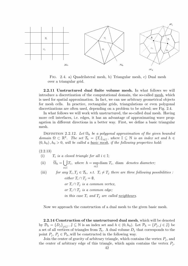
Fig. 2.4. a) Quadrilateral mesh, b) Triangular mesh, c) Dual meshover a triangular grid.

2.2.11 Unstructured dual finite volume mesh. In what follows we willintroduce a discretization of the computational domain, the so-called mesh, whichis used for spatial approximation. In fact, we can use arbitrary geometrical objectsfor mesh cells. In practice, rectangular grids, triangulations or even polygonaldiscretizations are often used, depending on a problem to be solved; see Fig. 2.4.

In what follows we will work with unstructured, the so-called dual mesh. Havingmore cell interfaces, i.e. edges, it has an advantage of approximating wave prop-agation in different directions in a better way. First, we define a basic triangularmesh.

Definition 2.2.12. Let Ωh be a polygonal approximation of the given boundeddomain Ω ⊂ R2. The set Th = {Ti}i∈I

, where I ⊆ N is an index set and h ∈(0, h0) , h0 > 0, will be called a basic mesh, if the following properties hold:

(i) Ti is a closed triangle for all i ∈ I;(2.2.13)

(ii) Ωh =⋃i∈I

Ti, where h = supi∈I

diam Ti, diam denotes diameter;

(iii) for any Ti, Tj ∈ Th, s.t. Ti �= Tj there are three following possibilities :

either Ti ∩ Tj = ∅,or Ti ∩ Tj is a common vertex,

or Ti ∩ Tj is a common edge;

in this case Ti and Tj are called neighbours.

Now we approach the construction of a dual mesh to the given basic mesh.

2.2.14 Construction of the unstructured dual mesh, which will be denotedby Dh = {Dj}j∈J

, J ⊆ N is an index set and h ∈ (0, h0). Let Ph = {Pj , j ∈ J} bea set of all vertices of triangles from Th. A dual volume Dj that corresponds to thepoint Pj , Pj ∈ Ph, will be constructed in the following way.

Join the center of gravity of arbitrary triangle, which contains the vertex Pj , andthe center of arbitrary edge of this triangle, which again contains the vertex Pj .

42

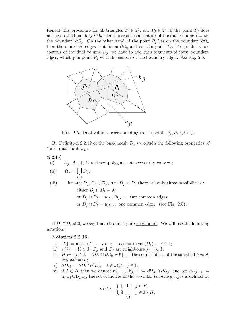
Repeat this procedure for all triangles Ti ∈ Th, s.t. Pj ∈ Ti. If the point Pj doesnot lie on the boundary ∂Ωh then the result is a contour of the dual volume Dj , i.e.the boundary ∂Dj . On the other hand, if the point Pj lies on the boundary ∂Ωh

then there are two edges that lie on ∂Ωh and contain point Pj . To get the wholecontour of the dual volume Dj , we have to add such segments of these boundaryedges, which join point Pj with the centers of the boundary edges. See Fig. 2.5.

Pj

DlD j

b

a jl

jl

Pl

Fig. 2.5. Dual volumes corresponding to the points Pj , P� j, � ∈ J.

By Definition 2.2.12 of the basic mesh Th, we obtain the following properties of“our” dual mesh Dh.

(i) Dj , j ∈ J, is a closed polygon, not necessarily convex ;(2.2.15)

(ii) Ωh =⋃j∈J

Dj ;

(iii) for any Dj , D� ∈ Dh, s.t. Dj �= D� there are only three possibilities :

either Dj ∩ D� = ∅,or Dj ∩ D� = aj� ∪ bj� . . . two common edges,

or Dj ∩ D� = aj� . . . one common edge; (see Fig. 2.5) .

If Dj ∩D� �= ∅, we say that Dj and D� are neighbours. We will use the followingnotation.

Notation 2.2.16.i) |Ti| := meas (Ti) , i ∈ I; |Dj | := meas (Dj) , j ∈ J;ii) s (j) := {� ∈ J; Dj and D� are neighbours } , j ∈ J;iii) H := {j ∈ J, ∂Dj ∩ ∂Ωh �= ∅} . . . the set of indices of the so-called bound-

ary volumes ;iv) ∂Dj� := ∂Dj ∩ ∂D�, � ∈ s (j) , j ∈ J;v) if j ∈ H then we denote aj,−1 ∪ bj,−1 := ∂Ωh ∩ ∂Dj , and set ∂Dj,−1 :=

aj,−1 ∪bj,−1; the set of indices of the so-called boundary edges is defined by

γ (j) :={ {−1} j ∈ H,

∅ j ∈ J \ H;43

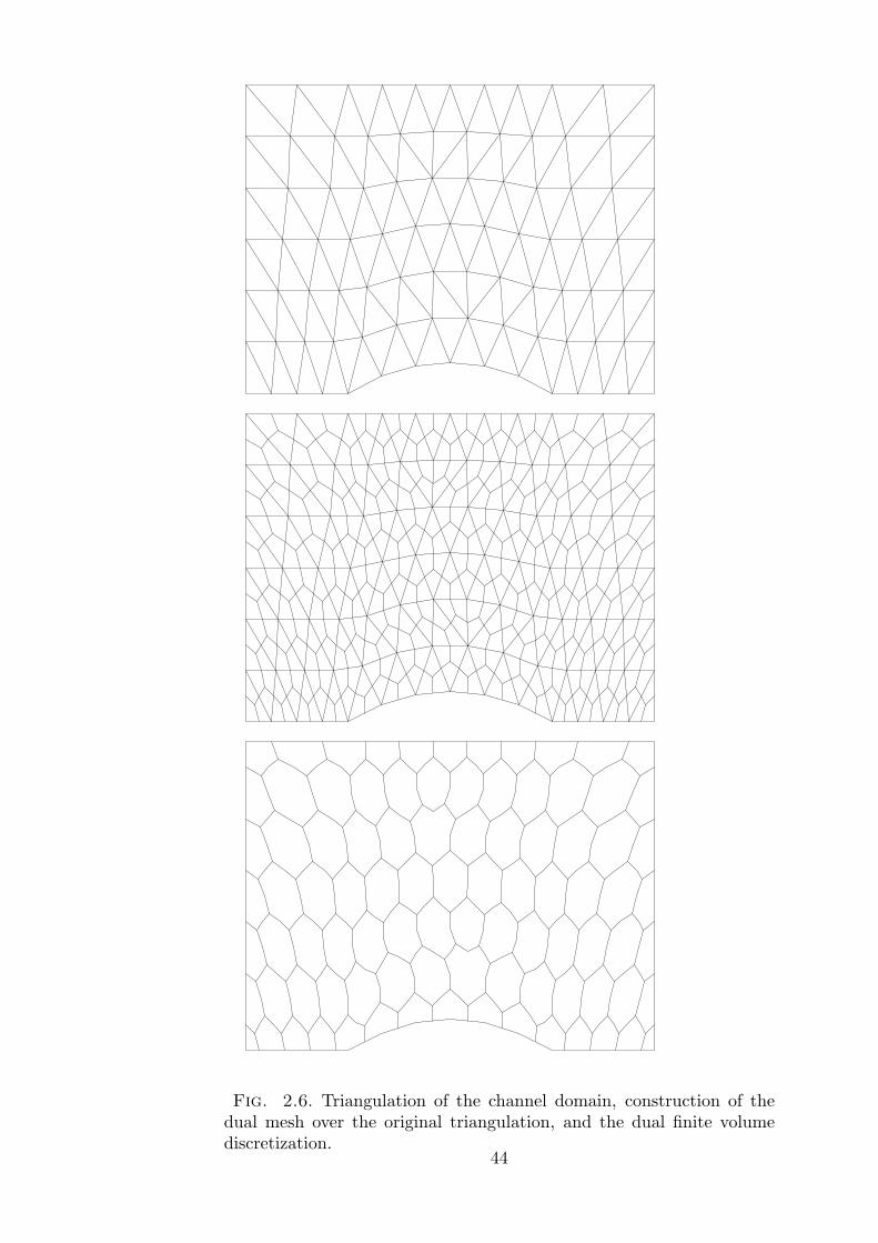
Fig. 2.6. Triangulation of the channel domain, construction of thedual mesh over the original triangulation, and the dual finite volumediscretization.

44

vi) S (j) := s (j) ∪ γ (j) , j ∈ J;vii) na

j� :=(na

xj�, nayj�

), j ∈ J, � ∈ S (j) . . . a unit outer normal to Dj on the

edge aj� ∈ ∂Dj�; analogously for the edge bj� ∈ ∂Dj� (if exists), nbj� :=(

nbxj�, n

byj�

);

viii) �j� := |∂Dj�|, j ∈ J, � ∈ S (j) ;ix) d := sup

j∈J

diam Dj .

Clearly,

(2.2.17) ∂Dj =⋃

�∈S(j)

∂Dj�, j ∈ J.

If we use suitable notation, i.e. aj� = a�j , and bj� = b�j , then

naj� = −na

�j , nbj� = −nb

�j , j ∈ J, � ∈ s (j) .

From the construction 2.2.14 it follows that

(i) if j ∈ J, � ∈ s (j) , then(2.2.18)

∂Dj� ={

aj� ∪ bj�, if j /∈ H or � /∈ H,

aj�, if j ∈ H and � ∈ H;(ii) if Ω = R

2 then H = ∅, γ (j) = ∅, S (j) = s (j) for all j ∈ J.

Further, we will define a discretization of time.

Definition 2.2.19. Let τ ∈ (0, τ0) , τ0 > 0. The set {tk; tk = k · τ,k = 0, . . . , N} , Nτ = T, 0 < T ≤ ∞ is called a time mesh and τ is called atime step.

To obtain a stable and convergent finite volume scheme we need to assume someregularity properties of the mesh, see e.g. [Ciarlet] for analogous assumptions inthe framework of the FEM.

Assumptions 2.2.20. The parameter of a mesh h → 0, whenever τ → 0, i.e.

(2.2.21) ∃ c1, c2 > 0 : 0 < c1 ≤ τ

h≤ c2, if τ, h → 0.

The triangles do not degenerate when h → 0, i.e.

(2.2.22) ∃ c3 > 0 : ∀i ∈ Ih

ρi≤ c3, if h → 0,

where ρi = diam Bi, Bi is the largest ball contained in Ti.

45

Remark 2.2.23. The regularity assumption (2.2.22) implies the following as-sumption,

∃ cV > 0 : supi∈I

h2

|Ti|≤ cV , if h → 0.

This can be easily verified by the fact that

|Ti| ≥ πρ2i .

The following remark says that the regularity properties of the basic triangularmesh are preserved for the dual one, too. Show it as an exercise!

Remark 2.2.24. If Assumptions 2.2.20 hold for the basic mesh Th, then thefollowing conditions are satisfied for the dual mesh Dh.

(2.2.25) ∃ c∗1, c∗2 > 0 : 0 < c∗1 ≤ τ

d≤ c∗2,

if τ → 0 and d = supj∈J

diam Dj → 0.

(2.2.26) ∃ c∗V > 0 : supj∈J

d2

|Dj |≤ c∗V , if d → 0.

2.2.27 Finite volume (FV) discretization with a cell-centered control vol-umes. The basic principle underlying a conservation law is that the total quantityof conservation variable in any region can be changed only due to flux through theboundaries. Mathematically, we integrate (2.2.1) over Dj × (tk, tk+1) , Dj is a dualcontrol volume and (tk, tk+1) is a chosen time interval. By Green’s theorem weobtain

(2.2.28)∫Dj

w (x, y, tk+1) =∫

Dj

w (x, y, tk) −∑

�∈S(j)

∫ tk+1

tk

∫∂Dj�

f1 (w) nx + f2 (w) ny.

In the cell-centered approach the discrete variables are associated with the gridpoints Pj ∈ Ph, or in fact, with the dual control volumes Dj ∈ Dh. We approximate

(2.2.29) w (x, y, tk) ≈ wkj = const. for any (x, y) ∈ Dj .

In the literature, see e.g. [Morton, Mayers], one can also meet a concept of cell-vertexfinite volumes. Here the discrete variables are associated with the values at verticesof the computational grid. Actually, the cell-vertex FVM can be reformulated asthe cell-centered FVM for the corresponding dual grid.Further, we need to approximate time integrals along the cell interfaces ∂Dj�. Inmany practical problems explicit numerical schemes are used, i.e.

(2.2.30)∫ tk+1

tk

∫∂Dj�

f1 (w) nx + f2 (w) ny ≈ τ

∫∂Dj�

f1(wk

)nx + f2

(wk

)ny.

46

Note that the implementation of explicit schemes is much easier than that ofimplicit ones, which would lead to a solution of algebraic systems at each time steptk. However, there is still a question how to approximate f1

(wk

), f2

(wk

)on the

boundary ∂Dj� of the control volume Dj , j ∈ J. To this end, a numerical fluxfunction H

(wk

j ,wk� ,nj�

), which approximates the amount of a quantity passing

through a unit of the area of ∂Dj� per a unit of time, is introduced. An importantthing is to choose this function in an appropriate way. Some properties of a suitablenumerical flux will be specified later. Now we introduce the following notation. If∂Dj� = aj� ∪ bj�, then the total flux through ∂Dj�, j ∈ J, � ∈ S (j), will be writtenas

(2.2.31) gj� (u,v) = H(u,v,na

j�

)|aj�| + H

(u,v,nb

j�

)|bj�|.

If ∂Dj� = aj�, j ∈ J, � ∈ s (j), which situation appears when j, � ∈ H, then

(2.2.32) gj� (u,v) = H(u,v,na

j�

)|aj�|.

The above discussion leads to the following approximations of the terms in (2.2.28) .

∫Dj

w (x, y, tk+1) ≈ |Dj |wk+1j ,

(2.2.33)

∫Dj

w (x, y, tk) ≈ |Dj |wkj ,

∑�∈S(j)

∫ tk+1

tk

∫∂Dj�

f1 (w) nx + f2 (w) ny ≈ τ∑

�∈S(j)

gj�

(wk

j ,wk�

).

Consequently, we derive the finite volume numerical scheme.

(2.2.34) wk+1j := wk

j − τ

|Dj |∑

�∈S(j)

gj�

(wk

j ,wk�

),

j ∈ J, k = 0, 1, . . . , to which the initial conditions are added

(2.2.35) w0j :=

1|Dj |

∫Dj

w0 (x, y) , j ∈ J.

The scheme (2.2.34) can be rewritten as any explicit numerical scheme in theform

(2.2.36) wk+1j := N

(wk

j ,{wk

� ; � ∈ S (j)})

.

The numerical scheme (2.2.36) is said to be conservative , if there is a continuousnumerical flux function H, s.t. (2.2.36) can be written in the form (2.2.34) (cf.(2.2.31), (2.2.32)).

47

As we have already pointed out the numerical flux should have some suitableproperties. We will assume the following.

H (u,v,n) : D × D × S1 → R4 is locally Lipschitz continuous :

(2.2.37)

(∀R > 0

)(∃ c = c (R) > 0

)(∀u,v,u∗,v∗ ∈ BR

)|H (u,v,n) − H (u∗,v∗,n)| ≤ c (R)

(|u − u∗| + |v − v∗|

),

where S1 is a unit sphere in R2 and BR = {x ∈ D; |x| ≤ R} .

H is consistent with an original equation (2.2.1) :(2.2.38)

H (u,u,n) = f1 (u) nx + f2 (u) ny, u ∈ D,n ∈ S1.

H is conservative :(2.2.39)

H (u,v,n) = −H (v,u,−n) , u,v,∈ D,n ∈ S1.

One can easily realize the following result.

Lemma 2.2.40. If (2.2.37)− (2.2.39) are fulfilled for the numerical flux functionH, then the same properties hold for the numerical flux function gj�, j ∈ J, � ∈S (j). It means that for any j ∈ J, � ∈ S (j), we have

(i) gj� : D × D → R4 is locally Lipschitz continuous :

(2.2.41)

(∀R > 0

)(∃ c1 = c1 (R) > 0

)(∀u,v,u∗,v∗ ∈ BR

)|gj� (u,v) − gj� (u∗,v∗)| ≤ c1 (R) �j�

(|u − u∗| + |v − v∗|

).

(ii) gj� is consistent :

gj� (u,u) = f1 (u) νxj� + f2 (u) νy�j , where u ∈ D,

νxj� = naxj�|aj�| + nb

xj�|bj�| for j /∈ H or � /∈ H;

νxj� = naxj�|aj�| for j, � ∈ H. Analogously for νy.

(iii) gj� is conservative:

gj� (u,v) = −g�j (v,u) , u,v ∈ D.

�

Theoretical results for the FVM. In the investigation of a numerical schemewe try to answer the following questions:

a) consistency of the method with the equation (2.2.1)b) stabilityc) convergence and order of the methodd) computational costs

48

In what follows we give an overview of some basic theoretical results for the FVM.Let us consider a Cauchy problem for (2.2.1) with the initial data (2.2.2), i.e. Ω =Rd.

We will deal first with the one-dimensional hyperbolic system (2.2.1), i.e. s ≥ 1,d = 1. Note that if d = 1 finite volume cells Dj reduce to simple one-dimensionalintervals (xj−1/2, xj+1/2).

Given an approximate solution wkj , j ∈ Z, k = 0, 1, . . . obtained by (2.2.34), we

introduce the piecewise constant function whτ (x, t), such that

(2.2.42) whτ (x, t) = wkj x ∈ Dj , t ∈ [tk, tk+1).

The convergence result of the finite volume method (2.2.34), (2.2.35) is establishedin the well-known Lax-Wendroff convergence theorem.

Theorem 2.2.43. (Lax, Wendroff (1960)) Let the numerical flux g�j in (2.2.34)be conservative and consistent. Moreover, let w0 ∈ L∞(R).1 Let us consider se-quences {hk}k, {τk}k; such that hk → 0+, τk → 0+ as k → ∞. Let us assume thatfor numerical solution wk ≡ whk,τk

the following conditions hold:

‖wk‖L∞(R×(0,∞)) ≤ c, k = 1, 2, . . .(2.2.44)

wk −→ w a.e. in R × (0,∞).

Then w is a weak solution of the Cauchy problem (2.2.1), (2.2.2) on R × [0,∞).

Proof. See, e.g. [Lax, Wendroff].�

In fact, condition (2.2.44) yields an assumption on the stability of the scheme.More precisely, we say that the numerical scheme (2.2.36) is (strongly) stable iffthe following inequality holds in appropriate norms

‖wk+1‖ ≤ ‖wk‖.

Thus, it implies that ‖wk‖ ≤ ‖w0‖ for each k = 1, 2, . . . . Note that for linearproblems L1 or L2-norms are suitable, whereas for nonlinear hyperbolic problemsstronger assumptions are needed, and the L∞ stability is required in order to getconvergence.

It should be pointed out here that due to the fact that we work with explicitmethods some additional assumption on the mesh size parameter h ∈ (0, h0) andtime step τ ∈ (0, τ0) has to be required. This is the so-called CFL (Courant-Friedrichs-Lewy) stability condition. It has to be taken in such a way that numericaldomain of dependence lies inside the physical one. We will explain this in thefollowing example.

Example: Consider the scalar one-dimensional equation

wt + awx = 0 R × [0,∞).

1Remind that we are using for the vector-valued functions simplified notation L∞(R) insteadof more precise L∞(R; Rs).

49

Let us use for the evaluation of numerical fluxes on the interfaces xj±1/2 the leftsided values of the approximate solution. We obtain the one-sided method

wk+1j = wk

j − aτ

h(wk

j − wkj−1), j ∈ Z, k = 0, 1, . . . .

Hence we have the following estimates in the discrete L1 norm

‖wk+1‖ = h∑

j

|wk+1j | ≤ h

∑j

∣∣∣(1 − aτ

h

)wk

j

∣∣∣ + h∑

j

∣∣∣aτ

hwk

j−1

∣∣∣ .If we now assume that the Courant-Friedrichs-Lewy number

aτ

hsatisfies

(CFL) 0 ≤ aτ

h≤ 1

the coefficients of wkj and wk

j−1 are both nonnegative, and we obtain the stabilitybound ‖wk+1‖ ≤ ‖wk‖. Note that the condition (CFL) requires in particular thata ≥ 0, since τ, h > 0. Thus, the one-sided method can only be used when a ≥ 0.We will recall this point also in the next subsection, where the notion of the upwindmethod is introduced, cf. (2.2.55). For a system of equations we would get

0 ≤ λkτ

h≤ 1

for all eigenvalues λk of A =Df(w)Dw

. This result is easily obtained from the

characteristic decomposition of the corresponding system, cf. (2.1.42).

Consider again the Cauchy problem (2.2.1), (2.2.2), i.e. Ω = R, s ≥ 1, d = 1. Letw be its classical solution. Substituting into (2.2.36) we obtain(2.2.45)w(xj , tk+1) = N

(w(xj , tk), {w(x�, tk); � ∈ S (j)}

)+ τεεεk

j , j ∈ N, k = 1, 2, . . . .

The quantity εεεkj is called a local truncation error of the scheme. We say that the

accuracy of the numerical scheme (2.2.36) is of order p in time and q in space, ifunder the assumption that the exact solution w of (2.2.1), (2.2.2) and the fluxf ≡ f1 are sufficiently smooth, there exist constants M,h0, τ0 such that

(2.2.46) |εεεkj | ≤ M(τp + hq), j ∈ N, k = 1, 2, . . . ; τ ∈ (0, τ0), h ∈ (0, h0).

We simply write εεεkj = O(τp + hq). The investigation of the local truncation error

and the order of accuracy is usually carried out by the Taylor expansion.

In Theorem 2.2.43 we have assumed that we already have a convergent subse-quence. Now we shall show how we can get it. Assume that the system (2.2.1) isone-dimensional and linear. Thus, we consider the following situation

∂w∂t

+ A∂w∂x

= 0 on R × (0,∞) ,

w(x, 0) = w0 on R.

The following fundamental Lax-Equivalence Theorem says that in the linear casestability and the local truncation error gives the global error.

50

Theorem 2.2.47. (Lax-Equivalence Theorem) Let us consider linear hyperbolicsystem (2.2.1). A linear numerical scheme (2.2.36) is stable and its local truncationerror is of order q in space and p in time if and only if the global error of numericalscheme is of order q and p in space and time, respectively, i.e.

‖w(tk) − wk‖L2(R) ≤ c(hq + τp) uniformly for k = 1, 2, . . . .

Proof. See, e.g. [Richtmeyr, Morton].�

The study of convergence of the FVM (2.2.34), (2.2.35) for nonlinear hyper-bolic problems is much more complicated. In fact, for general nonlinear hyperbolicsystems this question is still open. Consider nonlinear hyperbolic equation (2.2.1)with s = 1. Since we have to approximate discontinuous solutions, the choice of thefunction space in which we have to construct the converging sequence is the mostimportant problem. Following theoretical results of Glimm and Bressan, cf. Theo-rem 2.1.39, we find out that the space BV of functions with bounded total variationTV should be appropriate also in order to study convergence of discrete solutions.First we need to fix some additional notations.

As we have already shown in Section 2.1, the hyperbolic conservation laws admitnon-physical weak solutions. The entropy inequality (cf. Definition 2.1.30) must besatisfied in order to obtain a physically relevant solution. Similarly, in the discretecase the discrete entropy condition is required to guarantee a physically correctnumerical solution. To this end the entropy inequality is discretize. For simplicity,let us do this for a scalar equation (2.2.1) with s = 1.

Let U be the entropy function and Gj� be the discrete analogy of entropy fluxfunctions F1, F2, such that Gj�(u, u) = F1(u)νxj� +F2(u)νyj�, u ∈ D. Function Gj�

is the so-called numerical entropy flux . Discrete entropy inequality reads:

(2.2.48) U(wk+1

j

)≤ U

(wk

j

)− τ

|Dj |∑

�∈S(j)

Gj�

(wk

j , wk�

).

Note that the above inequality is only a discrete finite volume version of the“continuous” entropy inequality (2.1.28). If we regard the numerical flux gj� as a

function of the flux vector f =(

f1

f2

)and the solution w, i.e.

gj� = g (w, f) ,

then the numerical entropy flux can be chosen in the form

Gj� = g (U,F) ,

where F =(

F1

F2

)denotes the entropy flux vector.

In [Sonar (2)] it was shown that the above choice of discrete entropy flux leadsto a solution consistent with the Lax entropy condition (2.1.47). The general caseof systems (s > 1) is more complicated and the reader is referred to [Van der Burg].Practically control of discrete entropy inequality gives a very suitable tool to detectphysically incorrect features in a numerical solution, such as expansion shocks andwiggles near shock (see, e.g., [Van der Burg]).

Now we can approach formulation of the convergence result for nonlinear equa-tion (2.2.1) with s = d = 1. Its proof can be found e.g. in [Kroner].

51

Theorem 2.2.49. (sufficient conditions for convergence)Let w0 ∈ L1

loc(R)∩L∞(R). Let {wk ≡ whk,τk}k be a sequence of discrete solutions,

cf. (2.2.42), such that the following hold(1) numerical flux gj� is consistent and conservative(2)

‖wk‖L∞(R×(0,∞)) ≤ c, k = 1, 2, . . .

(3)TV (wk) ≤ c k = 1, 2, . . .

then there exists a w ∈ L1loc(R × [0,∞)) and a subsequence {wk′} such that

wk′ −→ w in L1loc(R × [0,∞)) as k′ −→ ∞

and w is a solution to (2.2.1), (2.2.2), s = d = 1, in the sense of distributions.Additionally if wk

j , j ∈ N, k = 0, 1, . . . satisfies the discrete entropy inequal-ity (2.2.48) then w satisfies the entropy condition (2.1.29). This solution is thenuniquely defined.

In the case of two-dimensional nonlinear scalar equation, i.e. (2.2.1) with s = 1,d = 2 the situation is more complicated. Convergence of the FVM for meshes,which consist of convex q−polygonals, was proved by Kroner and Rokyta [Kroner,Rokyta]. They used techniques of the measure valued solutions, the Young measuresand the compensated compactness arguments based on [DiPerna(1), (2)], [Tartar],etc. Its generalization to dual meshes was studied in [Lukacova]. In what followswe formulate the convergence result of the FVM for dual meshes. First, we needsome preliminary stability considerations.

We will suppose that the flux function g = gj� has the consistency, conservativityand Lipschitz continuity property (cf. (2.2.41)). However, it is still not enough forthe proof of stability and convergence of the FVM. We introduce the concept ofmonotonicity, which will play an important role.

Definition 2.2.50. (monotonicity) The scheme (2.2.34) is called monotone, ifthe functions

Hj(w) := wj −τ

|Dj |∑

�∈S(j)

gj�(wj , w�) j ∈ J,

where w = {wi}i∈J, are monotonously nondecreasing onMM = {w = {wi}i∈J, ‖w‖L∞(R2) ≤ M} for some M > 0. More precisely, if

w = {wi}i∈J, w∗ = {w∗

i }i∈J ∈ MM and w ≤ w∗ (i.e. wi ≤ w∗i for all i ∈ J), then

Hj(w) ≤ Hj(w∗).

Note that we have measured a sequence {wi} in the L∞ norm, instead of �∞.This is can be done since w = {wi} can naturally be associated with a functionw ∈ L∞(R2), such that w

∣∣∣Dj

= wj .

Clearly, monotonicity is stronger property than the boundedness of the totalvariation TV . For example, if f be a Lipschitz-continuous function on [a, b], whichis monotonously increasing then TV (f) = f(b) − f(a). Thus f ∈ BV ([a, b]).

We now approach to the proof of the L∞-stability property or the discrete maximumprinciple.

52

Theorem 2.2.51. (maximum principle) Let the approximate solution wk, k =0, 1, . . . , be defined by the numerical scheme (2.2.34), (2.2.35) for the scalar con-servation law (s = 1). Let w0 = {w0

j}j∈J ∈ MM , where M > 0. Let the scheme beconsistent (cf. (2.2.41) ii)) and monotone. Then we have for all k ∈ N:

‖wk‖L∞(R2) ≤ ‖w0‖L∞(R2).

Proof will be carried out by the mathematical induction. Let the desiredinequality holds for some k ∈ N. Obviously, it holds for k = 0. We denote m =‖wk‖L∞(R2) and construct w∗ = {w∗

j }j∈J s.t. w∗j = m for each j ∈ J. Then w∗ ∈

MM and wk ≤ w∗. Due to the monotonicity property we obtain Hj(wk) ≤ Hj(w∗)for each j ∈ J. Thus,

wk+1j = Hj(wk) ≤ Hj(w∗) = w∗

j − τ

|Dj |∑

�∈S(j)

gj�(w∗j , w∗

� )

= (using the consistency) = m − τ

|Dj |∑

�∈S(j)

f1(m)νxj� + f2(m)νyj�

= m − τ

|Dj |(f1(m)

∫∂Dj

nxdS + f2(m)∫

∂Dj

nydS)

= (using Green’s theorem) = m − τ

|Dj |(f1(m) · 0 + f2(m) · 0) = m.

We showed that wk+1j ≤ m for each j ∈ J, and we can analogously prove that

wk+1j ≥ −m by setting w∗

j = −m, j ∈ J. This leads to

|wk+1j | ≤ m = ‖wk‖L∞(R2) for each j ∈ J,

and finally‖wk+1‖L∞(R2) ≤ ‖wk‖L∞(R2).

�Now we can prove the L1-stability property.

Theorem 2.2.52. (L1-estimates) Let us assume that the scheme (2.2.34),(2.2.35), (s = 1), is conservative, consistent, monotone, with locally Lipschitz con-tinuous numerical flux (cf. (2.2.41)). Let w0 ∈ MM and ‖w0‖L1(R2) < ∞. We willsuppose that the following CFL-like stability condition holds:

(CFL)τc(M)|∂Dj |

|Dj |≤ 1, j ∈ J,

where c(M) is the constant of Lipschitz continuity of flux function. Then the schemeis L1-stable, i.e.

‖wk‖L1(R2) ≤ ‖w0‖L1(R2), k ∈ N.

53

Proof.Let us denote w∗ = {w∗

j }j∈J, w∗j = 0. Then clearly, due to the consistency

property we haveHj(w∗) = 0 for all j ∈ J.

Further, if we use the usual notation a+ = max(a, 0), a− = min(a, 0), then

(Hj(wk))+ ≤ Hj((wk)+)

and (Hj(wk))− ≥ Hj((wk)−), j ∈ J.

Here (wk)± = {(wkj )±}j∈J. We obtain

|wk+1j | = |Hj(wk)| = (Hj(wk))+ − (Hj(wk))− ≤ Hj((wk))+) − Hj((wk))−) =

= |wkj | −

τ

|Dj |∑

�∈S(j)

gj�((wkj )+, (wk

� )+) +τ

|Dj |∑

�∈S(j)

gj�((wkj )−, (wk

� )−).(*)

Our aim will be to show that τ∑

j∈J

∑�∈S(j) gj�(vj , v�) is absolutely convergent for

v = (w0)+ or v = (w0)−. Let us use Lipschitz continuity of the flux function:

τ∑j∈J

∑�∈S(j)

|gj�(vj , v�)| ≤ τ∑j∈J

∑�∈S(j)

|gj�(vj , v�) − gj�(w∗j , w∗

� )|

≤ τ∑j∈J

∑�∈S(j)

c(M)�j�(|vj | + |v�|)

≤ τc(M)∑j∈J

|∂Dj ||vj | + τc(M)∑j∈J

∑�∈S(j)

|∂D�||v�|.

Now we use the stability condition (CFL). Due to the regularity of basic triangu-lation there exist only finitely many, say q∗, neighbours of each dual volume Dj .Thus |S(j)| ≤ q∗ and the R.H.S. of the above inequality can be estimated by∑

j∈J

|Dj ||vj | + q∗∑j∈J

|Dj ||vj | < ∞,

because w0 ∈ L1(R2).By the conservativity property of gj� we find that∑

j∈J

∑�∈S(j)

gj�((w0j )+, (w0

� )+) =∑j∈J

∑�∈S(j)

gj�((w0j )−, (w0

� )−) = 0.

Hence, multiplying (*) by |Dj | and summing up over j ∈ J, leads to

‖w1‖L1(R2) ≤ ‖w0‖L1(R2).

The proof is finished by the mathematical induction.�

In the following theorem we formulate convergence result of the FVM for non-linear scalar conservation law (2.2.1), (2.2.2), s = 1, d = 2. We do not present itsproof since it would lead us behind the framework of this scriptum. Details can befound in [Lukacova].

54

Theorem 2.2.53. (convergence of the FVM on dual meshes) Let us assumethat an unstructured dual grid is constructed over general triangulation satisfyingAssumptions 2.2.20. Let w0 ∈ L∞(R2)∩L1(R2), w0 ∈ MM , the CFL-like condition(CFL) hold and wk

j , j ∈ J, k = 0, 1, . . . , be defined by the monotone finite volumescheme (2.2.34), (2.2.35), (s = 1). Let T > 0 be an arbitrary final time and Nsuch that Nτ = T. We suppose that for the numerical flux function the properties(2.2.41) hold and that analogous conditions to (2.2.41) hold also for the numericalentropy flux functions Gj�, j ∈ J, � ∈ S(j).

Moreover, we suppose that there exists β ∈ 〈0, 1) such that for all compact setsK ⊂ R2 uniformly in τ, h the numerical and entropy fluxes are controlled in thefollowing way

τβh

N∑k=0

∑j∈J:

Dj∩K �=0

∑�∈S(j)

|gj�(wkj , wk

� ) − gj�(wkj , wk

j )| ≤ c(K),

τβhN∑

k=0

∑j∈J:

Dj∩K �=0

∑�∈S(j)

|Gj�(wkj , wk

� ) − Gj�(wkj , wk

j )| ≤ c(K).

Finally, let the discrete entropy inequality hold

U(wk+1j ) − U(wk

j ) ≤ − τ

|Dj |∑

�∈S(j)

Gj�(wkj , wk

� )

for all entropies U and corresponding numerical entropy fluxes Gj�. Then

wk ⇀∗ w ∗-weakly in L∞(R2 × (0, T )) as k −→ ∞

and w is a Kruzhkov weak entropy solution of the problem (2.2.1), (2.2.2),s = 1, d = 2.

In the next subsection we will introduce several numerical flux functions gj� whichare used for practical computations. For example, the Engquist–Osher numericalscheme, cf. (2.2.59), satisfies all conditions of Theorem 2.2.53.

2.2.54 Godunov’s method. It was observed that a good numerical flux func-tion should include information propagated along characteristics, which leads tothe so-called upwinding. To describe this phenomenon let us consider a linearconvection equation in 1D.

∂w

∂t+ a

∂w

∂x= 0, x ∈ R, t > 0,

where a =const. is the speed of propagation of disturbances.Recall that in the case d = 1 the finite volumes reduce to Dj =

(xj−1/2, xj+1/2

);

xj = jh, j ∈ Z, h > 0, are mesh points, and xj±1/2 =xj + xj±1

2. The upwind

scheme reads:

(2.2.55) wk+1j = wk

j − τ

ha ·

⎧⎨⎩

(wkj − wk

j−1), a > 0,

(wkj+1 − wk

j ), a < 0.55

We can see that for approximation of ∂w∂x (xj , tk) we used finite difference approx-

imation oriented against the direction of propagation of disturbances.For the nonlinear case a = a(w) is not constant and the same approach does

not work directly. Then the local characteristic structure, obtained by solvinga Riemann problem (cf. (2.1.41)), is used to define a natural upwind method. Thiswas firstly used in 1959 by Godunov, who proposed a way to make use of thecharacteristic information within the framework of conservative method. Ratherthan attempting to follow characteristics backward in time, he suggested solvingthe following Riemann problem forward in time.

∂w

∂t+

∂f(w)∂x

= 0, x ∈ R, t > 0.(2.2.56)

w(x, 0) =

⎧⎨⎩

wL, x < 0,

wR, x > 0.

Here wL, wR ∈ R are given initial conditions. We know from Theorems 2.1.42,2.1.51 that under some assumptions on wL, wR, the Riemann problem (2.2.56) hasa unique entropy solution w (x, t) = wR (x/t;wL, wR). This result holds even in thecase of systems in 1D. Godunov numerical flux is defined in the following way

fG (u, v) = f(wR (0;u, v)

)and leads to the so-called Godunov’s method:

(2.2.57) wk+1j = wk

j − τ

h

[f(wR

(0;wk

j , wkj+1

))− f

(wR

(0;wk

j−1, wkj

))].

Although in some cases we know the exact solution wR of the Riemann problem(2.2.56), it is not the thruth in general. Thus, instead of wR we use an approximatesolution of (2.2.56), which leads us to the introduction of Riemann numerical flux orRiemann solver fR (u, v). The Godunov finite volume method can be then writtenin the following way

wk+1j = wk

j − τ

h

[fR

(wk

j , wkj+1

)− fR

(wk

j−1, wkj

)].

The aim is to construct a good numerical flux function, which is now denotedby fR(u, v). Using the method of characteristics it can be shown that if f ′ (w) =a (w) ≥ 0 for all w ∈ R, then wR (x/t;wL, wR) = wL, and if f ′ (w) = a (w) < 0 forall w ∈ R, then wR (x/t;wL, wR) = wR. Consequently, the Riemann numerical fluxis

fR (u, v) = f (u) if a ≥ 0,(2.2.58)

fR (u, v) = f (v) if a < 0.

This observation gives us a hint how to define Riemann numerical flux in generalnonlinear case. We split the flux function f (u) s.t.

f (u) = f+ (u) + f− (u) ,(f+

)′ ≥ 0,(f−)′ ≤ 0,

56

and definefR (u, v) := f+ (u) + f− (v) .

Finally, we obtain the following Godunov finite volume scheme:

wk+1j = wk

j − τ

h

[f+

(wk

j

)+ f−(wk

j+1) − f+(wkj−1) − f− (

wkj

)].

The numerical flux can be rewritten in the form

(2.2.59) fEO (u, v) =12(f (u) + f (v) −

∫ v

u

|a (q) |dq),

which is referred to as the Engquist–Osher numerical flux, see e.g. [Osher(1)],[Osher-Solomon].

Now we approach the generalization of these ideas to the case of Euler equationsin two space dimensions. Let P = P (w,n) be the flux function in 2D, i.e.

(2.2.60) P (w,n) := f1 (w) nx + f2 (w) ny,

w ∈ D,n ∈ S1, and the Jacobi matrix of P will be denoted by P = P (w,n) (cf.(2.2.8)).

One of the most useful properties of the Euler equations is the rotational invari-ance of their flux functions, i.e. if the matrix Λ is given by

Λ (n) =

⎛⎜⎝

1 0 0 00 nx ny 00 −ny nx 00 0 0 1

⎞⎟⎠ ,

then P (w,n) = Λ−1 (n) f1(Λ (n)w

)for all w ∈ D,n ∈ S1. The proof of this

statement follows from straightforward calculations. Due to this property the two-dimensional Euler equations can be transformed to a one-dimensional system in thedirection of the normal vector to a control volume Dj , j ∈ J. It is this property thatallows us to use of one-dimensional Riemann solvers to introduce two-dimensionalflux functions. Thus, in analogy to (2.2.59) one obtains that the numerical fluxfunction is

(2.2.61) HEO (u,v,n) :=12(P (u,n) + P (v,n) −

∫ v

u

|P (w,n) | dw).

Of course, this formula has sense only if the integral∫ v

uexists, but on the other hand

this gives us a good hint to derive numerical methods by suitable approximation ofthe integral

∫ v

u.

Before developing some methods, we state the following result.

Lemma 2.2.62. Let F ∈ C1 (Rs; Rs) be a homogeneous function of order one,i.e. F (αu) = αF (u) for all α ∈ R, α �= 0. Then

F (u) = A (u) · u,57

where A (u) =DF (u)

Du.

Proof.

A (u) · u =DF (u)

Du· u = lim

α→0

F (u + αu) − F (u)α

=

= limα→0

(1 + α)F (u) − F (u)α

= F (u) .

�It can be verified by straightforward calculations that for the Euler equations,

the flux functions f1, f2, and consequently P are homogeneous of order one. Hence,

f1 (u) = A1 (u) · u,(2.2.63)

f2 (u) = A2 (u) · u,

P (u,n) = P (u,n) · u.

Let us denote

(2.2.64) D± := diag

(λ±

1 , . . . , λ±4

),

where λ+i = max (λi, 0) , λ−

i = min (λi, 0).

(2.2.65) |D| = diag(|λ1|, . . . , |λ4|

).

(2.2.66) P± := T · D

± · T−1, |P| = T · |D| · T

−1.

Obviously, it holds

(2.2.67) P = P+ + P

−, |P| = P+ − P

−.

Now we approach approximation of the R. H. S. of (2.2.61).

a)∫ v

u

|P (w,n)| dw ≈∣∣∣∣P

(u + v

2,n

)∣∣∣∣ (v − u)(2.2.68)

b)12(P (u,n) + P (v,n)

)≈ P

(u + v2

,n)

=

=(using (2.2.63)

)= P

(u + v2

,n)u + v

2.

These approximations give the Vijayasundaram numerical flux;[Vijayasundaram]:

(2.2.69) HV (u,v,n) = P+(u + v

2,n

)u + P

−(u + v2

,n)v.

Using (2.2.58) and analogy with the one-dimensional case, one can derive theSteger–Warming numerical flux:

(2.2.70) HSW (u,v,n) = P+ (u,n)u + P

− (v,n)v.

If we use (2.2.68) a) and (2.2.61) we obtain the Van Leer numerical flux :

(2.2.71) HV L (u,v,n) =12

(P (u,n) + P (v,n) −

∣∣∣∣P(

u + v2

,n)∣∣∣∣ · (v − u)

).

58

Remarks 2.2.72.a) Let us note that in the Vijayasundaram scheme (cf. (2.2.69)) a partial upwind-

ing is included. The numerical flux between the volumes Dj and D� is computedaccording to the sign of local eigenvalues λi, i = 1, . . . , 4, of the matrix P and eitherwk

j or wk� is chosen for approximation.

More precisely, we take this one, which lies against the propagation of distur-bances. This upwinding is only partial, since the local eigenvalues are evaluated at

the central points : λi = λi

(wk

j +wk�

2

), j ∈ J, � ∈ S (j).

The fully upwind scheme is obtained by the Steger–Warming numerical flux func-tion (2.2.70). It is known that the full upwinding leads to the so-called numericaldiffusion, i.e. the leading order truncation error in the terms with second orderderivatives. As a result, discontinuities and shocks are smeared out.

b) It is easy to realize that all these numerical fluxes (2.2.69)− (2.2.71) have theproperties (2.2.37) − (2.2.39).

c) To derive the Vijayasundaram and the Steger–Warming numerical flux oneneeds the homogenity property (2.2.63) of the flux functions f1, f2. However, in thecase of a scalar conservation law (s = 1) this implies

(2.2.73) f ′1 (u) · u = f1 (u) , f ′

2 (u) · u = f2 (u) .

But in a scalar case this is fulfilled only for linear functions. We conclude thatthere makes no sense to consider these schemes for nonlinear scalar conservationlaw. This restriction does not include the Van Leer numerical flux.

d) Discrete entropy condition. Numerical as well as theoretical results, obtainedat least for scalar conservation law, show that the numerical solution obtained bythe method of Godunov’s type can violate entropy condition only in the case when

λk (wL) < 0 < λk (wR)

for some k = 1, 2, . . . , s.Clearly, the Lax entropy inequality (2.1.47) is not satisfied. Hence, discontinu-

ity, i.e. shock, is not an entropy solution. If the FVM approximates the Riemannproblem between wL and wR by means of the discontinuity it leads to an entropyviolating unphysical approximation. In this situation an exact solution of the Rie-mann problem (2.1.41) is a continuous sonic rarefaction wave.

To obtain the numerical solution, which satisfies the entropy inequality, we needto cure this case. This is referred to as entropy fix in literature. One approach,proposed in [Harten], [Osher (1)] is outlined here.

If one of the eigenvalues of the flux Jacobian matrix equals zero then approximatesolution can violate entropy condition. In order to prevent entropy violating acorrection to the eigenvalue is made. For the case of the Euler equations in 2D wehave the following eigenvalues (cf. 2.2.10)

λ1 = λ2 = v · n, λ3 = v · n + a, λ4 = v · n − a.59

Let λ := |v · n| + a be the maximum absolute eigenvalue. Then the entropy fixcorrection determines to put

|λk| := max{|λk|, δλ

}, k = 1, . . . , 4;

where δ > 0 is an entropy fix parameter, commonly chosen s.t. δ ∈ (0, 01; 1). Signof λk is unchanged.

e) The present schemes fall to the wide class of flux vector splitting methods. Inliterature one can meet other numerical schemes like Osher, Lax–Friedrichs, Roe,Mac Cormarck, Jameson ones, etc.

2.3. Boundary Conditions

In this section we want to derive suitable boundary conditions for solving theEuler equations in a bounded domain Ω ⊂ R2. In literature various approaches canbe found. We present here one, which is based on the method of characteristics.The general finite volume scheme reads (cf.( 2.2.43)):

(2.3.1) wk+1j = wk

j − τ

|Dj |∑

�∈S(j)

gj�

(wk

j ,wk�

), j ∈ J, k = 0, 1, . . . .

If j ∈ H and � ∈ γ (j) (i.e. � = −1, cf. (2.2.16)) then there is a problem how tocompute gj�

(wk

j ,wk�

), since there is no dual finite volume D� outside the domain

Ωh and the question is what is wk� ?

a) At first, if the edge S� ⊂ ∂Dj ∩ ∂Ωh, � ∈ γ (j) , (i.e. S� is either aj� or bj� (seeFig. 2.5)) is a part of the solid, impermeable wall, then the so-called slip boundaryconditions are imposed (cf. (1.4.7)).

(2.3.2) v · nj� = 0 on S�,

where nj� is an outer normal to Dj on S�.Then in numerical calculations we do not use numerical flux function gj�, but

we approximate the flux through S� in the following way

(2.3.3)∫

S�

(f1 (w) nx + f2 (w) ny

)dS =

=∫

S�

{(v1 nx + v2 ny)w + p ·

⎛⎜⎝

0nx

ny

0

⎞⎟⎠}

dS ≈ |S�| pj

⎛⎜⎝

0nx

ny

0

⎞⎟⎠ .

Hence, we extrapolate the value of the pressure from the point Pj to the wholeboundary edge S�. The numerical flux H on the solid part of the boundary S� ⊂

60

∂Ωh ∩ ∂Dj is then defined by the formula

(2.3.4) H(wk

j ,wk� ,nj�

):= pk

j

⎛⎜⎝

0nxj�

nyj�

0

⎞⎟⎠ ,

and the numerical flux function gj� is computed in the usual way

(2.3.5) gj�

(wk

j ,wk�

)= H

(wk

j ,wk� ,na

j�

)|aj�| + H

(wk

j ,wk� ,nb

j�

)|bj�|.

b) If the edge S� ⊂ ∂Dj ∩ ∂Ωh, � ∈ γ (j) , lies on inlet or outlet part of theboundary, we use the heuristical approach proposed in [Feistauer]. Let a computa-tional domain Ω be represented as (−∞, 0) and solve the linearized one-dimensionalconservation system

(2.3.6)∂w∂t

+ A∂w∂x

= 0 on (−∞, 0) × (0,∞) .

By the hyperbolicity property one gets

(2.3.7) A = T · D · T−1, D = diag (λ1, . . . , λs) .

From (2.3.6) and (2.3.7) we find the system of s independent equations

∂zi

∂t+ λi

∂zi

∂x= 0, i = 1, 2, . . . , s, on (−∞, 0) × (0,∞) .

These equations can be solved by the method of characteristics. If λi > 0, thenthe initial value, which is prescribed at {t = 0, x < 0}, is propagated along thecharacteristics with the slope λi > 0 to the half-line {x = 0, t > 0} and the value ofthe solution is uniquely determined here.

On the other hand, if λi < 0, then the characteristics starting at {t = 0, x < 0}do not intersect the half line {x = 0, t > 0} and the boundary conditions should beprescribed here.

These ideas are heuristically extended to the case of the Euler equations. Henceon S� ⊂ ∂Dj ∩ ∂Ωh, a part of inlet or outlet, we prescribe np quantities charac-terizing the state vector wk

� , which corresponds to the boundary edge S�; np is anumber of negative local eigenvalues of the matrix P

(wk

j

). Further, we extrapolate

ne quantities from the point Pj to the edge S�, ne is a number of positive localeigenvalues of P

(wk

j

).

Now, there is a question : Which quantities should be prescribed and which onesare extrapolated? There is the following classical approach.

On inlet, i.e. vkj · nj� < 0, for the case of supersonic flow

(−vk

j · nj� > akj

), ak

j

is a local speed of sound computed from wkj , we have (cf. (2.2.10) for eigenvalues

of the Euler equations):

(2.3.8, i) λ1 = λ2 < 0, λ3 < 0, λ4 < 0 =⇒ np = 4, ne = 0,61

and we prescribe boundary condition for ρ, v1, v2, p to characterize wk� .

For the case of subsonic flow(−vk

j · nj� < akj

):

(2.3.8, ii) λ1 = λ2 < 0, λ3 > 0, λ4 < 0 =⇒ np = 3, ne = 1.

We prescribe ρ, v1, v2 and extrapolate p from the point Pj .On outlet, i.e. vk

j · nj� > 0, for the case of supersonic flow(vk

j · nj� > akj

)we

have :

(2.3.8, iii) λ1 = λ2 > 0, λ3 > 0, λ4 > 0 =⇒ np = 0, ne = 4.

We extrapolate ρ, v1, v2, p from Pj . For the case of subsonic flow(vk

j · nj� < akj

):

(2.3.8, iv) λ1 = λ2 > 0, λ3 > 0, λ4 < 0 =⇒ np = 1, ne = 3,

and we extrapolate ρ, v1, v2 from Pj and prescribe p.

This discussion leads to the definition of wk� , which is the state vector corre-

sponding to the boundary edge S�. Now we can evaluate H(wk

j ,wk� ,nj�

), i.e. the

flux through the edge S�, and consequently we compute gj�

(wk

j ,wk�

)by (2.3.5).

2.4 Second Order Method

In practise it is often important to derive a good approximation of the exact,often unknown, solution. Thus, the numerical scheme should be enough accurateand posse an adequate rate of dissipation to give physically relevant entropy solutionand has a higher order accuracy to obtain sharp shock waves in the correct solution.We first discuss the generalized MUSCL methodology, which is used to increasespatial accuracy of the basic finite volume scheme (2.2.34) , (2.2.35). Thus, insteadof (2.2.34) we use the following scheme

(2.4.1) wk+1j := wk

j − τ

|Dj |∑

�∈S(j)

gj�

(wk

j�, wk�j

), j ∈ J,

where wkj�, w

k�j are values of a new higher order function wh at the boundary ∂Dj�

at time step tk.MUSCL approach requires to replace the piecewise constant function wh, which

is defined on dual volumes by a higher order function. Since we want to get thesecond order scheme (in the sense of truncation error), we choose a piecewise linearrecovery function wh, which will be linear on dual volumes and discontinuous atthe boundaries of dual volumes. Thus, wh will be recovered from wh in such a waythat we have

(2.4.2) wh

∣∣∣Dj

= wh (Pj) =1

|Dj |

∫Dj

wh (x, y) .

62

Now we show one possibility how to construct this linear recovery not on theconservative variables, but separately on the physical variables ρ, v1, v2, p. Letq ∈ {ρ, v1, v2, p}, and qh be a piecewise constant function on the dual volumes,which corresponds to some physical variable q. We will define qh, i.e. a piecewiselinear recovery function on the dual volumes, in the following way:

(2.4.3) qh (x, y) := qh

∣∣∣Dj

+ (gradhqh)∣∣∣Dj

· (x − xj , y − yj)T

,

(x, y) ∈ Dj , j ∈ J, (xj , yj) are coordinates of the point Pj ;Pj ∈ Ph. Since qh

∣∣∣Dj

=

qh (Pj), the piecewise linear recovery function qh will be determined by (2.4.3) , if

we define (gradhqh)∣∣∣Dj

.

Now we realize that from piecewise constant function on the dual volumes qh onecan construct a continuous, piecewise linear function on triangles. More precisely,let

(2.4.4) Xh ={

ωh ∈ C(Ω; R

); ωh

∣∣∣Ti

∈ Pi (Ti) , i ∈ I

}

be the space of linear finite element functions, and

(2.4.5) Dh ={

qh : Ω → R; qh

∣∣∣Dj

∈ P0 (Dj) , j ∈ J

}

be the space of piecewise constant finite volume functions. Here Pk (·) denotes thespace of polynomials of order not greater than k, k = 0, 1.

The basis of Xh is formed by the functions wj , j ∈ J, s.t. wj (P�) = δj�, wj ∈ Xh.Further, the basis of Dh is formed by the characteristic functions of dual finitevolumes Dj , denoted by dj , j ∈ J.

There exists a bijection Lh : Xh → Dh, called the mass-lumping operator anddefined in the following way

(2.4.6) Lhωh =∑j∈J

ωh (Pj) dj ,

where ωh =∑

j∈J

(ωh (Pj) · wj

)∈ Xh. Let L (j) = {k ∈ I; ∃Tk ∈ Th : Pj ∈ Tk} .

Using the inverse mapping to Lh, i.e. Πh = L−1h , we obtain a function Πhqh =∑

j∈J

qh

∣∣∣Dj

wj , which is piecewise linear on triangles. This allows us to compute the

so-called averaged gradient :

(2.4.7) (gradh qh)∣∣∣Dj

:=1

|Dj |∑

k∈L(j)

∫Tk∩Dj

grad Πh qh =

=1

|Dj |∑

k∈L(j)

(grad Πh qh)∣∣∣Tk

· |Tk ∩ Dj |.

Now we can use (2.4.3) to define the values of qh at the boundary ∂Dj�, � ∈ S (j),

of the dual volume Dj . Let zaj� =

(xa

j�, yaj�

), zb

j� =(xb

j�, ybj�

)be the midpoints of

63

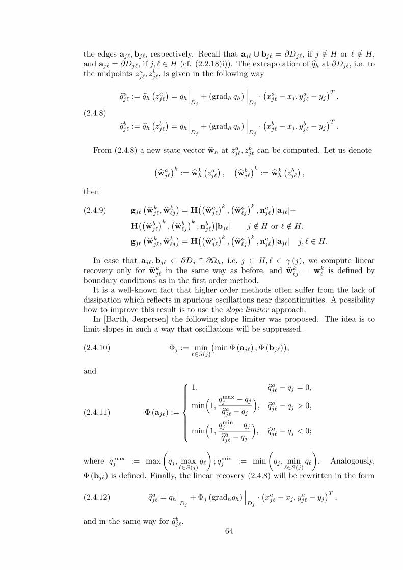
the edges aj�,bj�, respectively. Recall that aj� ∪ bj� = ∂Dj�, if j /∈ H or � /∈ H,and aj� = ∂Dj�, if j, � ∈ H (cf. (2.2.18)i)). The extrapolation of qh at ∂Dj�, i.e. tothe midpoints za

j�, zbj�, is given in the following way

qaj� := qh

(zaj�

)= qh

∣∣∣Dj

+ (gradh qh)∣∣∣Dj

·(xa

j� − xj , yaj� − yj

)T,

qbj� := qh

(zbj�

)= qh

∣∣∣Dj

+ (gradh qh)∣∣∣Dj

·(xb

j� − xj , ybj� − yj

)T.

(2.4.8)

From (2.4.8) a new state vector wh at zaj�, z

bj� can be computed. Let us denote

(wa

j�

)k := wkh

(zaj�

),

(wb

j�

)k:= wk

h

(zbj�

),

then

gj�

(wk

j�, wk�j

)= H

((wa

j�

)k,(wa

�j

)k,na

j�

)|aj�|+(2.4.9)

H((

wbj�

)k,(wb

�j

)k,nb

j�

)|bj�| j /∈ H or � /∈ H.

gj�

(wk

j�, wk�j

)= H

((wa

j�

)k,(wa

�j

)k,na

j�

)|aj�| j, � ∈ H.

In case that aj�,bj� ⊂ ∂Dj ∩ ∂Ωh, i.e. j ∈ H, � ∈ γ (j), we compute linearrecovery only for wk

j� in the same way as before, and wk�j = wk

� is defined byboundary conditions as in the first order method.

It is a well-known fact that higher order methods often suffer from the lack ofdissipation which reflects in spurious oscillations near discontinuities. A possibilityhow to improve this result is to use the slope limiter approach.

In [Barth, Jespersen] the following slope limiter was proposed. The idea is tolimit slopes in such a way that oscillations will be suppressed.

(2.4.10) Φj := min�∈S(j)

(min Φ (aj�) ,Φ (bj�)

),

and

(2.4.11) Φ (aj�) :=

⎧⎪⎪⎪⎪⎪⎪⎨⎪⎪⎪⎪⎪⎪⎩

1, qaj� − qj = 0,

min(1,

qmaxj − qj

qaj� − qj

), qa

j� − qj > 0,

min(1,

qminj − qj

qaj� − qj

), qa

j� − qj < 0;

where qmaxj := max

(qj , max

�∈S(j)q�

); qmin

j := min(

qj , min�∈S(j)

q�

). Analogously,

Φ (bj�) is defined. Finally, the linear recovery (2.4.8) will be rewritten in the form

(2.4.12) qaj� = qh

∣∣∣Dj

+ Φj (gradhqh)∣∣∣Dj

·(xa

j� − xj , yaj� − yj

)T,

and in the same way for qbj�.

64

A discrete scheme is said to be TVD (total variation diminishing), if for thesequence wk =

{wk

j

}j∈J

, k = 0, 1, . . . , the total variation, i.e. TV(wk

)=∑

j∈J

�∈S(j)

|wkj − wk

� |, satisfies the condition

(2.4.13) TV(wk

)≥ TV

(wk+1

), k = 0, 1, . . . .

The described construction of second order method is based on a one-dimensionalsecond order TVD extension of the first order scheme, it can be considered asa second order TVD-MUSCL scheme, see e.g. [Osher(2)], [Rostard, Stoufflet] forfurther results.

Although it can be even impossible to prove for fully nonlinear systems that ourmultidimensional scheme is the second order, the number of numerical experimentsconfirm the reliability of the method and the higher order behaviour of numericalsolutions, see e.g. [Kroner, Noelle, Rokyta] for some convergence results of thehigher order FVM. In Fig. 2.7 the comparison of the first and the second orderFVM and the corresponding exact solution is given. We have chosen the two-dimensional Riemann problem, cf. Fig. 2.3, and plot the y = 0-cut. It can beobserved that the second order method approximates extrema of the solution in abetter way and resolves discontinuity more sharply than the first order scheme.

0 0.5 1 1.50

0.2

0.4

0.6

0.8

1

1.2First and second order FVM vs. exact solution

rho − exact rho − 1st FV − 50x50rho − 2nd FV − 50x50

Fig. 2.7. Comparison of the first and second order FVM.

In order to obtain fully higher order FVM it is further necessary to considerbetter approximation in time. In fact, we apply the so-called method of lines andtreat separately spatial and time approximation. Thus, let us consider the followingsystem of ordinary differential equations with respect to time

(2.4.14)dw(t)

dt= F(w(t)),65

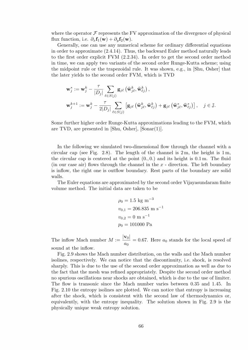
where the operator F represents the FV approximation of the divergence of physicalflux function, i.e. ∂xf1(w) + ∂yf2(w).

Generally, one can use any numerical scheme for ordinary differential equationsin order to approximate (2.4.14). Thus, the backward Euler method naturally leadsto the first order explicit FVM (2.2.34). In order to get the second order methodin time, we can apply two variants of the second order Runge-Kutta scheme; usingthe midpoint rule or the trapezoidal rule. It was shown, e.g., in [Shu, Osher] thatthe later yields to the second order FVM, which is TVD

w∗j := wk

j − τ

|Dj |∑

�∈S(j)

gj�

(wk

j�, wk�j

),

wk+1j := wk

j − τ

2|Dj |∑

�∈S(j)

[gj�

(wk

j�, wk�j

)+ gj�

(w∗

j�, w∗�j

)], j ∈ J.

Some further higher order Runge-Kutta approximations leading to the FVM, whichare TVD, are presented in [Shu, Osher], [Sonar(1)].

In the following we simulated two-dimensional flow through the channel with acircular cap (see Fig. 2.8). The length of the channel is 2 m, the height is 1 m,the circular cap is centered at the point (0., 0.) and its height is 0.1 m. The fluid(in our case air) flows through the channel in the x - direction. The left boundaryis inflow, the right one is outflow boundary. Rest parts of the boundary are solidwalls.

The Euler equations are approximated by the second order Vijayasundaram finitevolume method. The initial data are taken to be

ρ0 = 1.5 kg m−3

v0,1 = 206.835 m s−1

v0,2 = 0 m s−1

p0 = 101000 Pa

The inflow Mach number M :=|v0|a0

= 0.67. Here a0 stands for the local speed of

sound at the inflow.Fig. 2.9 shows the Mach number distribution, on the walls and the Mach number

isolines, respectively. We can notice that the discontinuity, i.e. shock, is resolvedsharply. This is due to the use of the second order approximation as well as due tothe fact that the mesh was refined appropriately. Despite the second order methodno spurious oscillations near shocks are obtained, which is due to the use of limiter.The flow is transonic since the Mach number varies between 0.35 and 1.45. InFig. 2.10 the entropy isolines are plotted. We can notice that entropy is increasingafter the shock, which is consistent with the second law of thermodynamics or,equivalently, with the entropy inequality. The solution shown in Fig. 2.9 is thephysically unique weak entropy solution.

66

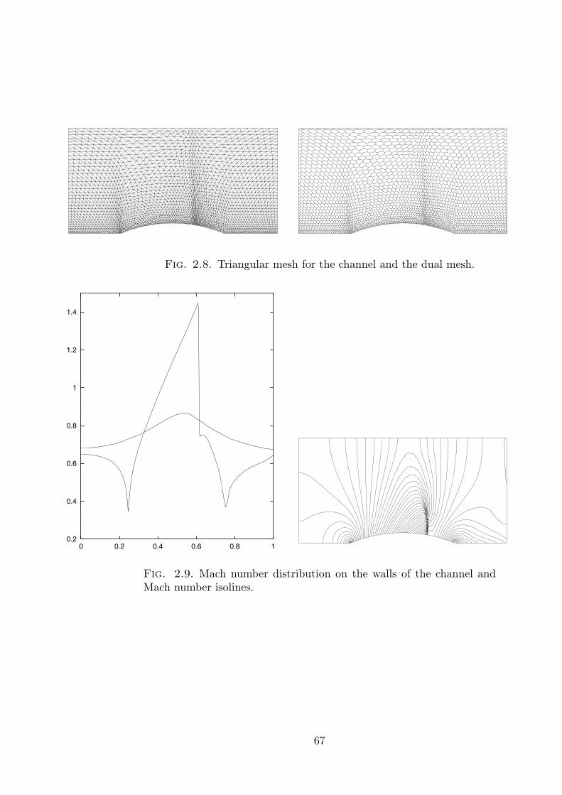
Fig. 2.8. Triangular mesh for the channel and the dual mesh.

0.2

0.4

0.6

0.8

1

1.2

1.4

0 0.2 0.4 0.6 0.8 1

Fig. 2.9. Mach number distribution on the walls of the channel andMach number isolines.

67

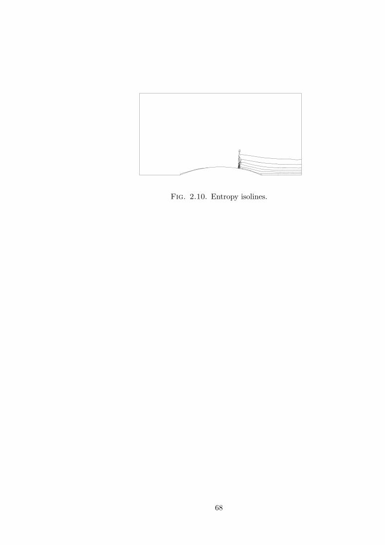
Fig. 2.10. Entropy isolines.

68

CHAPTER III

TUTORIALS

In this chapter we give a list of open problems for students’ individual work orfor the use in seminars.

Exercise 1.Show that in R3 the following equality holds

rot rot = grad div − div grad.

Exercise 2. (1D Euler equations in conservative and primitive variables)Consider the system of the Euler equations in 1D in conservative variables

(ρ, ρu, e)

∂tρ + ∂x(ρu) = 0,

∂t(ρu) + ∂x(ρu2 + p) = 0,

∂te + ∂x((e + p)u) = 0

with the so-called state equation for ideal polytropic gas

p = (κ − 1)(e − ρu2/2) κ �= 1.

Let (ρ, ρu, e) be a solution to the Euler equations in conservative variables. Showthat under some regularity assumptions, i.e. smoothness of the solution, it is alsoa solution to the Euler equations in the so-called primitive variables (ρ, u, p)

∂tρ + ∂x(ρu) = 0,

∂tu + u∂xu +∂xp

ρ= 0,

∂tp + ρa2∂xu + u∂xp = 0,

where

a :=√

κp

ρ

denotes the speed of sound. Which regularity conditions have to be assumed?

69

Exercise 3. (Euler equations)Compute for the above one-dimensional Euler equations Jacobian A, all eigen-

values and corresponding eigenvectors. Compare the results with those given inChapter 2.2 for the full two-dimensional system. How it will be for the three-dimensional system?

Programming exercises:

Exercise 4. (One-dimensional convection-diffusion equation)The so-called convection-diffusion equation is a simple mathematical model

of fluid dynamics which describes fluid flowing in a given direction and take intoaccount viscous (or diffusive) effects. In one space dimension we have

− εu′′(x) + bu′(x) = f(x) x ∈ (0, 1)(3.1)

u(0) = 0, u(1) = 0.(3.2)

Here ε is a small parameter (physically ε ≈ 1/Re), b is a given velocity of the flow(transport or advection parameter). Taking b > 0 means that fluid flows from leftto right. By f we denote some outer forces which cause fluid movement, e.g. heatsources.

Mathematically (3.1), (3.2) gives a boundary value problem for linear ODE ofthe second order. That is we need two boundary conditions. Now taking ε → 0,e.g. ε = 10−10, we get as an approximate model to equation (3.1) the followingequation

(3.3) bu′(x) = f(x) x ∈ (0, 1).

This is now a linear ordinary differential equation of the first order and we canprescribe just one boundary condition. Actually, if b > 0 we should take the leftboundary value of (3.2) and conversely, if b < 0 we take the right value of (3.2).

Equation (3.1) with 0 < ε � 1 is called singularly perturbed equation. Itis a small perturbation of (3.3), but this small perturbation changes characterof the equation completely (from the first order to the second order). Singularperturbation problems cause numerical difficulties because the solution changesrapidly over a very small interval in space. In this region derivatives of u(x) arelarge, giving rise to large errors in our finite difference approximations.

In what follows let us consider, for simplicity, the following equation

− εu′′(x) + u′(x) = 1 x ∈ (0, 1)(3.4)

u(0) = 0, u(1) = 0.(3.5)

The exact solution to this problem is

u(x) = x +1 − ex/ε

e1/ε − 1.

70

0

0.2

0.4

0.6

0.8

1

0 0.2 0.4 0.6 0.8 1

x + (1-exp(x/1))/(exp(1) -1)x

0

0.2

0.4

0.6

0.8

1

0 0.2 0.4 0.6 0.8 1

x + (1-exp(x/0.1))/(exp(1/0.1) -1)x

0

0.2

0.4

0.6

0.8

1

0 0.2 0.4 0.6 0.8 1

x + (1-exp(x/0.01))/(exp(1/0.01) - 1)x

Fig. 3.1. Exact solution for various values of ε = 1, 0.1, 0.01 and thesolution for ε = 0.

This solution is plotted for different values of ε in the Fig. 3.1.

Discretize (3.4) by means of the finite difference method. Take an equidistantmesh on the interval (0, 1) of the mesh size h. Take the boundary conditions (3.5)at U0 ≡ u(0) = 0 and UN ≡ u(1) = 0, where N = 1/h. You will obtain a linearalgebraic system of the following type

AU = R,

with a sparse three-diagonal matrix A and U = (U1, . . . , UN ), Ui ≈ u(ih). Solve thislinear system for U! (You can use, e.g., some appropriate MATLAB subroutines.)Note that you can use the sparsity of the matrix A and do not need to save all of(N − 1) × (N − 1) entries into memory.

(1) Compare three possibilities to approximate the first derivative of u′(x).Take a fixed ε (e.g. ε = 0.1, 0.01) and plot the exact and approximatesolutions for several values of h.

(2) Plot logarithm of the error ln‖u−U‖ over ln(h); (e.g. take h = 1/10, h =1/25, h = 1/100). Here ‖u − U‖ = maxi=1,...,N |u(ih) − Ui|.

(3) What is the leading order local truncation error in finite difference approxi-mation of (3.4)? Where can you see its influence in the graphs of numericalsolution?

The following exercises 5.- 8. have to be solved using the finite volume methodof the wave propagation algorithm, the so-called CLAWPACK (Version 4.0) (Con-servation Law Package). See: http://www.amath.washington.edu/ claw

Exercise 5. (Viscous Burgers equation)Solve the one-dimensional viscous Burgers equation

qt +(

12q2

)x

= εqxx, x ∈ [−2, 3].

71

The finite volume solver of Roe (“Roe solver”) is based on the linearization qt +Aiqx = 0 with Ai = 1

2 (qi−1 + qi). Note that for this scalar problem Ai = λ1i and

this is the correct shock speed in the case that the solution is a shock wave. Forthe wave propagation algorithm we set

W1i := qi − qi−1,

λ1i :=

12(qi−1 + qi),

A−Δqi := min(λ1i , 0)W1

i = −12q2i−1,

A+Δqi := max(λ1i , 0)W1

i =12q2i .

In this case we have A−Δqi + A+Δqi = 12

(q2i − q2

i−1

)= f(qi) − f(qi−1).

In order to solve the viscous part the so-called operator splitting is implementedin the CLAWPACK and the scr1 subroutine solves the diffusion equation

qt = εqxx

over a time step. This is done using the Crank-Nicolson method, which requiressolving a tridiagonal linear system of equations for the whole update of qi.

Solve the Burgers equation with the extrapolation boundary conditions and thefollowing initial data

q(x, 0) = 1 x < 0

q(x, 0) = 0 x > 0

or

q(x, 0) = 0 x < 0

q(x, 0) = 1 x > 0

Test the behavior of solution for several viscosity coefficients ε = 0, 1, 0.1, 0.01,0.001. Plot solutions at several time steps!

Exercise 6. (Acoustics equation)The two-dimensional acoustics equation for the pressure perturbation p and ve-

locities u and v can be written as

qt + Aqx + Bqy = 0,

where

q =

⎛⎝ p

uv

⎞⎠ , A =

⎛⎝ 0 K 0

1/ρ 0 00 0 0

⎞⎠ , B =

⎛⎝ 0 0 K

0 0 01/ρ 0 0

⎞⎠ .

Solve the acoustics equation with the radially symmetric initial data p(x, y, 0) =P0(r), u = v = 0 where r =

√x2 + y2. Set P0(r) = 1 − 0.1(cos(4πr) − 1). The

72

solution should remain radially symmetric. Moreover you can test the accuracy ofthe two-dimensional scheme by computing solution on a very fine grid by solvingthe one-dimensional equations

Pt + KUr = −aU/r

ρUt + Pr = 0,

where U is the radial velocity and a =√

K/ρ. Solve this system on a very finegrid using 1D solver and then solve 2D equations on a sequence of N ×N grids forN = 10, 20, 40, 80 on [−1, 1] × [−1, 1]. The end time is set to be t = 0.4. Plot thecomparisons between the “exact” 1D solution and scatter plot of the 2D numericalsolutions. These latter are obtained by the first as well as the second order FVschemes. Compute numerical errors between the reference and numerical solutionsin L1 as well as in L∞-norms for all N × N grids.

Exercise 7. (Acoustics in heterogeneous medium)Now we suppose that sound speed varies in x, y due to variations in the material

parameters ρ and K. We have then the system

qt + A(x, y)qx + B(x, y)qy = 0,

where

q =

⎛⎝ p

uv

⎞⎠ , A =

⎛⎝ 0 K(x, y) 0

1/ρ(x, y) 0 00 0 0

⎞⎠ , B =

⎛⎝ 0 0 K(x, y)

0 0 01/ρ(x, y) 0 0

⎞⎠ .

In this example we model the propagation of a plane wave when striking an interfaceof two materials. As an initial data take a planar wave propagating in some directionat an angle to the interface

p(x, y, 0) = 0.5 + cos(πr/0.1) if r =√

(x − 0.25)2 + (y + 0.4)2 < 0.1, 0 else

u(x, y, 0) = 1.5, v(x, y, 0) = 1.

Set the interface variables as follows

ρ(x, y) = ρL = 1.0, a(x, y) =√

K(x, y)/ρ(x, y) = aL = 1.0 x < 0.5,

ρ(x, y) = ρR = 4.0, a(x, y) =√

K(x, y)/ρ(x, y) = aR = 0.5 x > 0.5

or

ρ(x, y) = ρL = 1.0, a(x, y) = aL = 1.0 x < y/5 + 0.4,

ρ(x, y) = ρR = 4.0, a(x, y) = aR = 0.5 x > y/5 + 0.4.

The end time is set to be t = 0.64 and the computational domain is [0, 1.5]× [−1, 1].Use 300× 200 grid. Compare pressure isolines of the numerical solutions as well asthe graphs along cross sections at x = 0.6 and x = 1.0 for both types of interfaces.

73

Note that in order to plot graph along the cross sections you have to modify slightlyprocedure claw/clawpack/2d/lib/out2.f in order to get only output data along thespecified cross-section. Use extrapolated boundary conditions. Compare first andsecond order methods.

Exercise 8. (Euler equations with shock in entropy)In this example we model a shock wave hitting sinusoidal variation in entropy

(i.e. variation in density with constant pressure). The system of the Euler equationsreads

qt + f(q)x = 0,

where the vector of conservative variables and the fluxes are

q :=

⎛⎝ ρ

ρue

⎞⎠ , f(q) :=

⎛⎝ ρu

ρu2 + p(e + p)u

⎞⎠ , x ∈ [−5, 5], t ∈ [0, 2].

In order to close the system the state equation of ideal gas is used. Take thefollowing initial data

ρ(x, 0) = 3.857, u(x, 0) = 2.629, p(x, 0) = 10.333, x < −4

ρ(x, 0) = 1 + 0.2 sin(5x), u(x, 0) = 0, p(x, 0) = 1, x ≥ −4.

Plot ρ, u and p on fine and coarse grid using 200 and 4000 grid cells. Com-pare results for the first and second order methods. Use extrapolated boundaryconditions on the left and the right boundary, i.e. x = ±5.

Exercise 9. (Two-dimensional nonlinear convection-diffusion equation)Combined finite volume - finite element methodSolve the following two-dimensional convection-diffusion equation

ut + uux + uuy = εΔu, (x, y) ∈ [−1, 1] × [−2, 2],(3.6)

u(x, y, 0) = 10 (x2 + y2)1/2 < 0.4= 1 else

∂u

∂n= 0 Neumann B.C.

Use regular mesh consisting of square cells

Ωij ≡ [(i − 1/2)h, (i + 1/2)h] × [(j − 1/2)h, (j + 1/2)h]

= [xi−1/2, xi+1/2] × [yj−1/2, yj+1/2],

where indices i, j ∈ Z, and h > 0 is the mesh size parameter.Approximate equation (3.6) with the so-called operator splitting finite element-

finite volume method. It means to divide time step [tn, tn+1] into two half timesteps. Solve in the first time step [tn, tn+1/2] a pure advection equation

ut + uux + uuy = 074

with the finite volume method

Un+1/2ij := Un

ij −Δt

2h2

[Hi+1/2,j − Hi−1/2,j + Hi,j+1/2 − Hi,j−1/2

].

Here Hi±1/2,j denotes a numerical flux function on the right/left cell interface.Analogous notation holds for y-direction. Try the following methods: second orderLax-Wendroff scheme as well as first order Lax-Friedrichs and Vijayasundarammethods.

In the second step [tn+1/2, tn] solve the rest parabolic equation

(3.7) ut = εΔu

with linear conforming finite element method using the so-called dual mesh to theoriginal mesh {Ωij}i,j∈Z. Dual mesh is a staggered mesh, i.e. “shifted mesh”. Itconsists of squares {Ωα,β}α,β∈Z, where (α, β) are vertices of the original mesh. Letϕij be a finite element test function corresponding to the vertex (i, j) of the dualmesh {Ωα,β}α,β∈Z. It is a bilinear function, which equals 1 at the vertex (i, j) andzero at other vertices (k, l). Show that the finite element approximation of (3.7)leads to the following scheme

Un+1ij := U

n+1/2ij − Δt

4h2ε(Un+1/2

i−1j + Un+1/2i+1j + U

n+1/2ij−1 + U

n+1/2ij+1 − 4U

n+1/2ij ).

In order to approximate integrals of any continuous function f(x, y) over one meshcell the trapezoidal quadrature is used, i.e.

∫Ωα,β

f(x, y)dx =h2

4

∑k,�:(xk,y�)∈Ωα,β

fk�.

Note that gradients of test functions are constant on each dual mesh cell Ωα,β .

Plot three-dimensional representations of the solution u at three different timeinstances, e.g. T = 0.1, 0.5, 1. Try several viscosity parameters, e.g. ε = 10, 1, 0.01,0.001. Which stability condition, i.e. condition on relationship between Δt and h,has to be fulfilled?

75

REFERENCES

Barth T.J., Jespersen D.C., The design and application of upwind schemes on un-structured meshes, AIAA paper 366, 1989.

Bressan, A., Hyperbolic Systems of Conservation Laws, The One-DimensionalCauchy Problem, Oxford University Press 2000.

Ciarlet P.G., The Finite Element Method for Elliptic Problems, North - Holland,Amsterdam, 1979.

Courant R., Friedrichs K.O., Supersonic Flow and Shock Waves, Springer - Verlag,New York - Heidelberg - Berlin, 1976.

Di Perna R. J. (1), Measure-valued solutions to conservation laws, Arch. RationalMech. Anal. 88, 1985, pp. 223 - 270.

Di Perna R. J. (2), Convergence of approximate solutions to conservation laws,Arch. Rational Mech. Anal. 82, 1983, pp. 27 - 70.

Feistauer M., Mathematical Methods in Fluid Dynamics, Longman Scientific &Technical , Harlow, 1993.

Glimm J. Solutions in the large for nonlinear hyperbolic systems of equations,Comm. Pure Appl. Math., 18, 1965, pp. 95 - 105.

Godlewski E., Raviart P.A.(1), Hyperbolic Systems of Conservation Laws, Mathe-matiques & Applications, S.M.A.I., Ellipses, Paris , 1991.

Godlewski E., Raviart P.A.(2), Numerical Approximation of Hyperbolic Systems ofConservation Laws, Springer Verlag, New York, 1996.

Gurtin M.E., An Introduction to Continuum Mechanics, Academic Press, NewYork, 1981.

Hirsch C., Numerical Computation of Internal and External Flows, Vols 1.,2., JohnWiley & Sons Ltd., Chichester, 1984.

Harten A., On a class of high resolution total-variation-stable finite differenceschemes, SIAM J. Numer. Anal. 21, 1984, pp. 1 - 23.

Kroner D., Numerical Schemes for Conservations Laws, Wiley Teubner, Stuttgart1997.

Kroner D., Rokyta M., Convergence of upwind finite volume schemes for scalarconservation laws in 2D , SIAM J. Numer. Anal. 31(2), 1994, pp. 324-343.

76

Kroner D., Noelle S., Rokyta M., Convergence of higher order upwind finite vol-ume schemes on unstructured grids for scalar conservation laws in several spacedimensions. Numer. Math. 71 (4), 1995, pp. 527-560.

Kruzhkov S.N., First order quasilinear equations in several independent variables,Math. USSR Sbornik 10, 1970, pp. 217 - 243.

Kufner A., John O., Fucık S., Function Spaces, Academia, Prague, 1977.

Ladyzhenskaya O.A., The Mathematical Theory of Viscous Incompressible Flow,Nauka, Moscow, 1970, (in Russian).

Lax P.D. (1), Shock waves and entropy, In: Contributions to Nonlinear Funct.Analysis, (Zarontonello E.A. - ed.), Academic Press, 1971, pp. 603 - 634.

Lax P.D. (2), Hyperbolic Systems of Conservation Laws and the Mathematical The-ory of Shock Waves, SIAM, 1973.

Lax P.D., Wendroff B., Systems of conservation laws, Comm. Pure Appl. Math.13, 1960, pp. 217 - 237.

LeVeque R.J. (1), Numerical Methods for Conservation Laws, Birkhauser, Basel -Boston - Berlin, 1990.

LeVeque R.J. (2), Finite Volume Methods for Hyperbolic Problems, Cambridge Uni-versity Press, Cambridge, 2002.

Li J., Zhang T., Yang S., The Two–dimensional Riemann Problem in Gas Dy-namics, Pitman Monographs and Surveys in Pure and Applied Mathematics 98,Longman, 1998.

Li J., Lukacova - Medvid’ova M., Warnecke G., Evolution Galerkin schemes ap-plied to two-dimensional Riemann problems for the wave equation system, DiscreteContin. Dyn. Syst. 9(3), 2003, pp. 559-576.

Lukacova - Medvid’ova M., Numerical Solution of Compressible Flows, PhD Dis-sertation, Charles University Prague, 1994.

Lukacova - Medvid’ova M., Morton K.W., Warnecke G., Finite Volume EvolutionGalerkin Methods for Euler Equations of Gas Dynamics, Int. J. Numer. Meth.Fluids 40 (3-4), 2002, pp. 425-434.

Lukacova-Medvid’ova M., Saibertova J., Warnecke G., Finite Volume EvolutionGalerkin Methods for Nonlinear Hyperbolic Systems, J. Comput. Phys. 183(2),2002, pp. 533-562.

Malek J., Necas J., Rokyta M., Ruzicka M., Weak and Measure-valued Solutions toEvolutionary Partial Differential Equations, Applied Mathematics and Mathemat-ical Computation, 13, Chapman & Hall, London, 1996.

Morton K.W., Mayers D.Numerical Solution of Partial Differential Equations,Cambridge University Press, Cambridge, 1994.

Necas J., Les methodes directes en theorie des equations elliptiques, Academia,Prague, 1967.

Osher S. (1), Riemann solvers, the entropy condition, and difference approxima-tions, SIAM J. Numer. Anal. 21 (2), 1984, pp. 217 - 235.

77

Osher S. (2), Convergence of generalized MUSCL schemes, SIAM J. Num. Anal.22, 1985, pp. 947 - 961.

Osher S., Solomon F., Upwind difference schemes for hyperbolic systems of conser-vation laws, Math. Comp. 38, 1982, pp. 339 - 374.

Richtmeyr R.D., Morton K.W., Difference Methods for Initial-value Problems,Wiley-Interscience, 1967.

Rostand Ph., Stoufflet B., TVD schemes to compute compressible viscous flowson unstructured grids, In: Nonlinear Hyperbolic Equations - Theory, ComputationMethods and Applications (Ballman J., Jeltsch R. - eds.), Notes on Numerical FluidMechanics 24, Vieweg, Braunschweig, 1989.

Schochet S., The compressible Euler equations in a bounded domain: existence ofsolutions and incompressible limit, Comm. Math. Phys. 104, 1986, pp. 49 - 75.

Shu, C.-W., Osher S., Efficient implementation of essentially non-oscillatory shockcapturing schemes II, J. Comput. Phys. 83, 1989, pp. 32 - 78.

Sever M., Uniqueness failure for entropy solutions of hyperbolic systems of conser-vation laws, Comm. Pure Appl. Math. 42, 1989, pp. 173 - 183.

Smoller J., Shock Waves and Reaction-Diffusion Equations, Springer, 1983.

Sonar Th. (1), Mehrdimensionale ENO-Verfahren, Teubner Stuttgart, 1997.

Sonar Th. (2), Nichtlineare Dissipationsmodelle und Entropie - Production infiniten Differenzenverfahren, PhD Dissertation, Univ. Stuttgart, 1991.

Tartar L.C., The compensated compactness method applied to systems of conserva-tion laws, In: Systems of Nonlinear P.D.E.’s (J. Ball - ed.), D. Reidel PublishingCompany, 1983, pp. 263 - 285.

Temam R., Navier–Stokes Equations, North - Hollad, Amsterdam - New York -Oxford, 1977.

Toro E.F., Riemann Solvers and Numerical Methods for Fluid Dynamics, Springer-Verlag, 1999.

Valli A., Mathematical results for compressible flows, Preprint Univ. degli Studi diTrento, 1992.

Van der Burg J.W., Numerical Techniques for Transonic Flow Calculations, PhDDissertation, University of Twente, 1992.

Vijayasundaram G., Transonic flow simulation using an upstream centered schemeof Godunov in finite elements, J. Comp. Phys. 63, 1986, pp. 416 - 433.

Wada Y., Kubota H., Ishiguro T., Ogawa S., A fully implicit high-resolution schemefor chemically reacting compressible flows, In: Nonlinear Hyperbolic Equations -Theory, Computation Methods, and Applications (Ballman J., Jeltsch R. - eds.),Notes on Numerical Fluid Mechanics 24, Vieweg, Braunschweig, 1989.

Warnecke G., Analytische Methoden in der Theorie der Erhatungsgleichungen,Teubner, Stuttgart-Leipzig, 1999.

Wesseling P., Principles of Computational Fluid Dynamics, Springer Verlag Berlin-Heidelberg, 2001.

78

Yosida K., Nonlinear Analysis, Springer - Verlag, New York, 1974.

Zeidler E., Nonlinear Functional Analysis and its Applications 1. - 4., Springer -Verlag, New York, 1985 - 1989.

Zienkiewicz O.C., Taylor R.L., Finite Element Method, Vol 3. Fluid Dynamics,Butterworth-Heinemann, Bristol, 2000.

Zenısek A., Nonlinear elliptic and evolution problems and their finite element ap-proximations, Computational Mathematics and Applications, Academic Press, Lon-don, 1990.

79