2.29 numerical fluid mechanics lecture 9 slides · pdf file2.29 numerical fluid mechanics pfjl...
TRANSCRIPT
PFJL Lecture 9, 1Numerical Fluid Mechanics2.29
2.29 Numerical Fluid Mechanics
Spring 2015 – Lecture 9
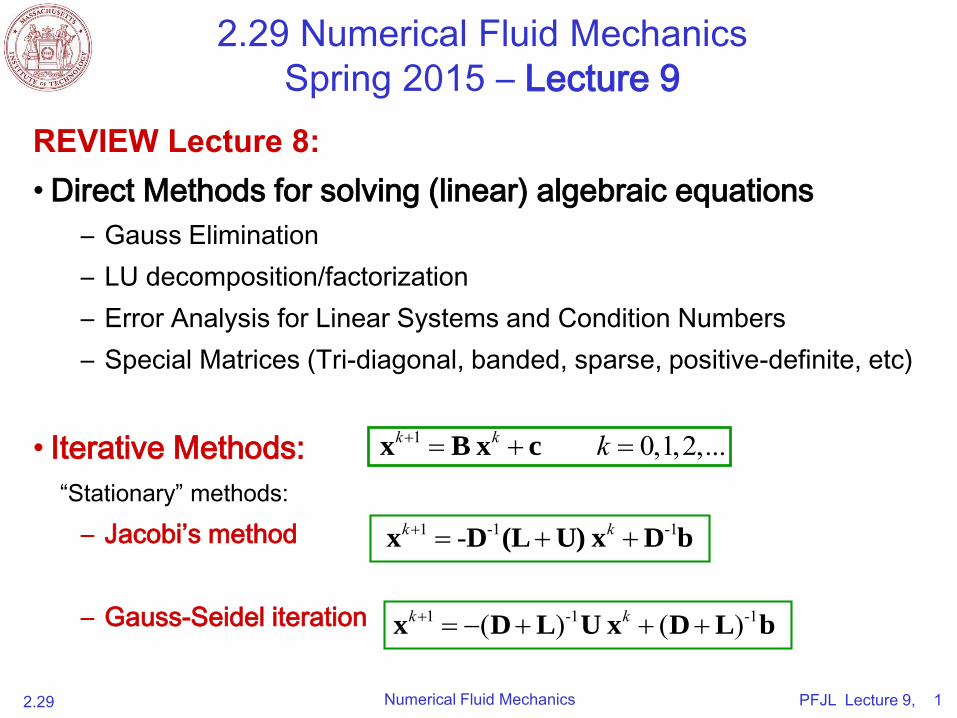
REVIEW Lecture 8:• Direct Methods for solving (linear) algebraic equations
– Gauss Elimination
– LU decomposition/factorization
– Error Analysis for Linear Systems and Condition Numbers
– Special Matrices (Tri-diagonal, banded, sparse, positive-definite, etc)
• Iterative Methods:
– Jacobi’s method
– Gauss-Seidel iteration
1 0,1,2,...k k k x B x c
1 -1 -1-k k x D (L U) x D b
1 -1 -1( ) ( )k k x D L U x D L b
“Stationary” methods:
PFJL Lecture 9, 2Numerical Fluid Mechanics2.29
2.29 Numerical Fluid Mechanics
Spring 2015 – Lecture 9REVIEW Lecture 8, Iterative Methods Cont’d:
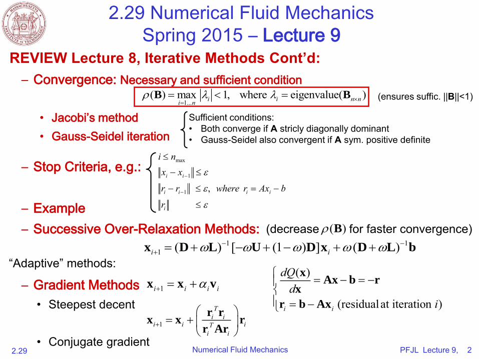
– Convergence: Necessary and sufficient condition
• Jacobi’s method
• Gauss-Seidel iteration
– Stop Criteria, e.g.:
– Example
– Successive Over-Relaxation Methods:
– Gradient Methods
• Steepest decent
• Conjugate gradient
1...( ) max 1, where eigenvalue( )i i n ni n
B B (ensures suffic. ||B||<1)
i nmax
xi xi1
ri ri1 , where ri Axi b
ri
Sufficient conditions:• Both converge if A stricly diagonally dominant• Gauss-Seidel also convergent if A sym. positive definite
(decrease for faster convergence)1 1
1 ( ) [ (1 ) ] ( )i i
x D L U D x D L b
( ) B
1i i i i x x v( )
(residualat iteration )i i
dQd
i
xAx b r
x
r b Ax
1
Ti i
i i iTi i
r rx x r
r Ar
“Adaptive” methods:
PFJL Lecture 9, 3Numerical Fluid Mechanics2.29
TODAY (Lecture 9)
• End of (Linear) Algebraic Systems
– Gradient Methods and Krylov Subspace Methods
– Preconditioning of Ax=b
• FINITE DIFFERENCES
– Classification of Partial Differential Equations (PDEs) and examples
with finite difference discretizations
– Error Types and Discretization Properties
• Consistency, Truncation error, Error equation, Stability, Convergence
– Finite Differences based on Taylor Series Expansions
• Higher Order Accuracy Differences, with Example
• Taylor Tables or Method of Undetermined Coefficients
– Polynomial approximations
• Newton’s formulas, Lagrange/Hermite Polynomials, Compact schemes
PFJL Lecture 9, 4Numerical Fluid Mechanics2.29
References and Reading Assignments
• Chapter 14.2 on “Gradient Methods”, Part 8 (PT 8.1-2), Chapter 23 on “Numerical Differentiation” and Chapter 18 on “Interpolation” of “Chapra and Canale, Numerical Methods for Engineers, 2006/2010/2014.”
• Chapter 3 on “Finite Difference Methods” of “J. H. Ferzigerand M. Peric, Computational Methods for Fluid Dynamics. Springer, NY, 3rd edition, 2002”
• Chapter 3 on “Finite Difference Approximations” of “H. Lomax, T. H. Pulliam, D.W. Zingg, Fundamentals of Computational Fluid Dynamics (Scientific Computation). Springer, 2003”
PFJL Lecture 9, 5Numerical Fluid Mechanics2.29
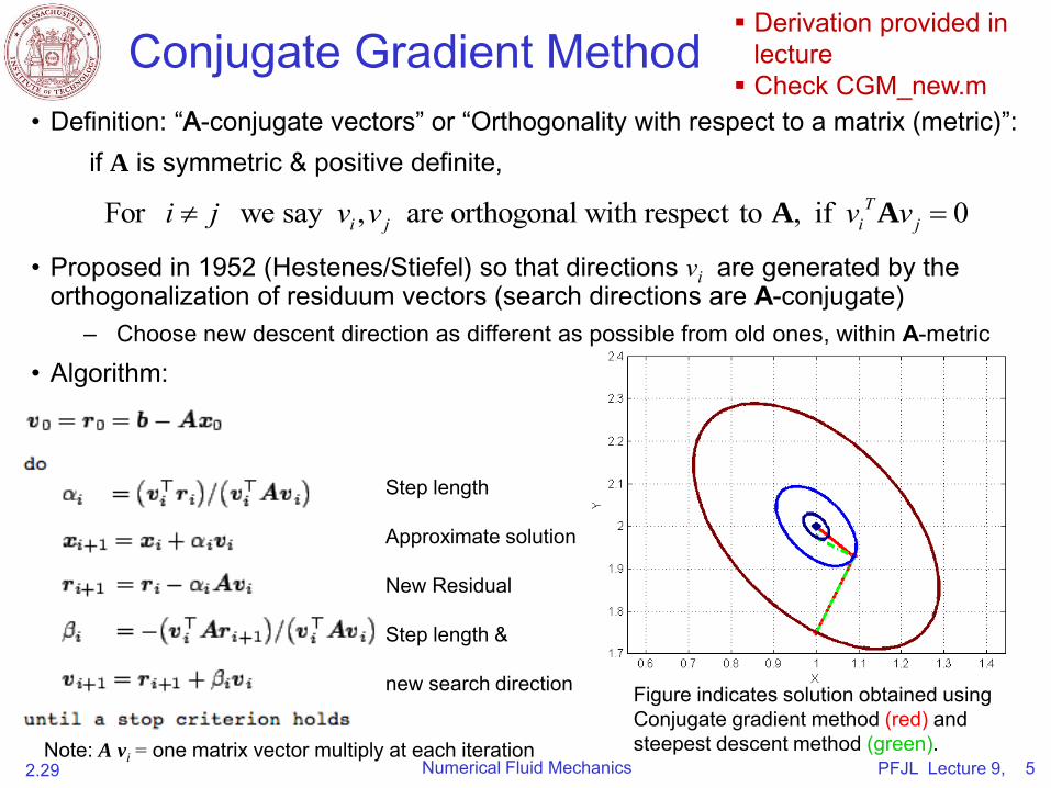
Conjugate Gradient Method
• Definition: “A-conjugate vectors” or “Orthogonality with respect to a matrix (metric)”:
if A is symmetric & positive definite,
• Proposed in 1952 (Hestenes/Stiefel) so that directions vi are generated by the orthogonalization of residuum vectors (search directions are A-conjugate)
– Choose new descent direction as different as possible from old ones, within A-metric
• Algorithm:
For we say , are orthogonal with respect to , if 0Ti j i ji j v v v v A A
Figure indicates solution obtained using Conjugate gradient method (red) and steepest descent method (green).
Step length
Approximate solution
New Residual
Step length &
new search direction
Note: A vi = one matrix vector multiply at each iteration
Derivation provided in lecture
Check CGM_new.m
PFJL Lecture 9, 6Numerical Fluid Mechanics2.29
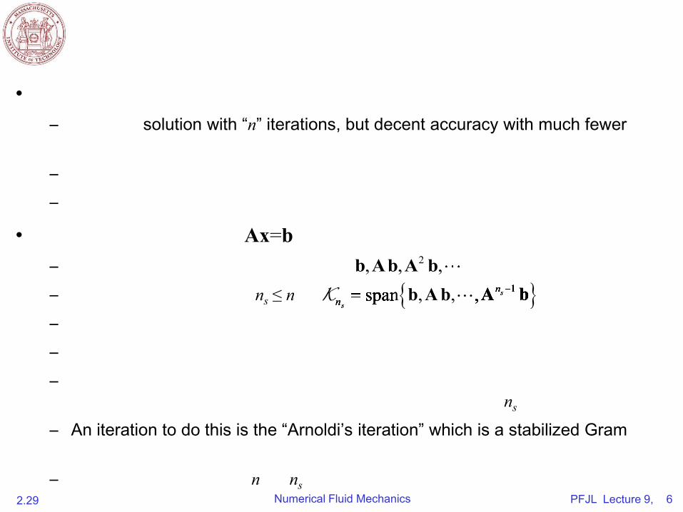
•
– solution with “n” iterations, but decent accuracy with much fewer
–
–
• Ax=b–
– ns ≤ n
–
–
–
ns
– An iteration to do this is the “Arnoldi’s iteration” which is a stabilized Gram
– n ns
1span , , , s
s
nn
b A b A b1span , , , nb A b A b1b A b A b1span , , ,b A b A bspan , , , sb A b A bsnb A b A bn b A b A bspan , , ,
sn
2, , ,b Ab A b
PFJL Lecture 9, 7Numerical Fluid Mechanics2.29
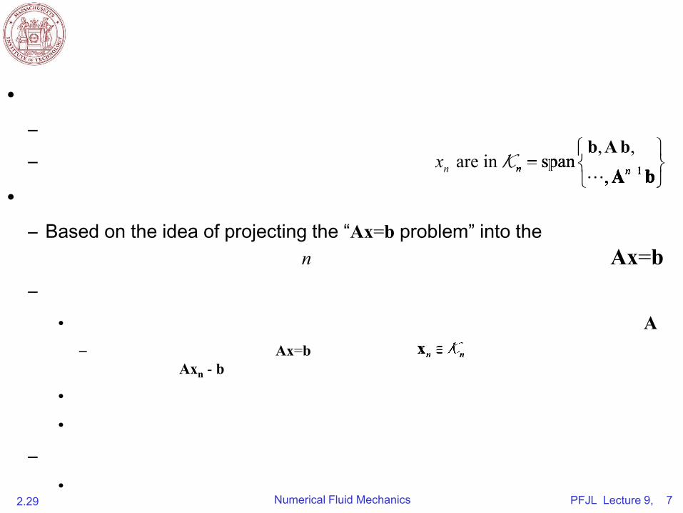
•
–
–
•
– Based on the idea of projecting the “Ax=b problem” into the
n Ax=b–
• A– Ax=b
Axn - b
•
•
–
•
n nxn nx
1
, , are in span
,n n nx
b A bA b 1 1n n
, , 1 1
1 1n n
n n A b
1
1A b1
1n
nA bn
n A b 1 1
1 1A b1 1
1 1n n
n nA bn n
n n
A b
are in spann n are in spann n are in span are in span are in span
PFJL Lecture 9, 8Numerical Fluid Mechanics2.29
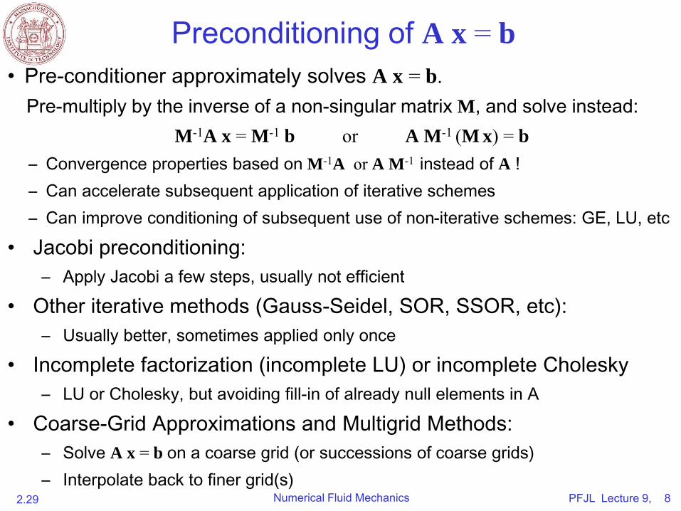
Preconditioning of A x = b• Pre-conditioner approximately solves A x = b.
Pre-multiply by the inverse of a non-singular matrix M, and solve instead:
M-1A x = M-1 b or A M-1 (M x) = b
– Convergence properties based on M-1A or A M-1 instead of A !
– Can accelerate subsequent application of iterative schemes
– Can improve conditioning of subsequent use of non-iterative schemes: GE, LU, etc
• Jacobi preconditioning:
– Apply Jacobi a few steps, usually not efficient
• Other iterative methods (Gauss-Seidel, SOR, SSOR, etc):
– Usually better, sometimes applied only once
• Incomplete factorization (incomplete LU) or incomplete Cholesky
– LU or Cholesky, but avoiding fill-in of already null elements in A
• Coarse-Grid Approximations and Multigrid Methods:
– Solve A x = b on a coarse grid (or successions of coarse grids)
– Interpolate back to finer grid(s)
PFJL Lecture 9, 9Numerical Fluid Mechanics2.29
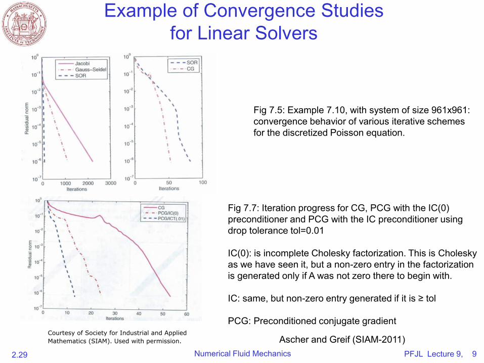
Example of Convergence Studies
for Linear Solvers
Fig 7.5: Example 7.10, with system of size 961x961: convergence behavior of various iterative schemes for the discretized Poisson equation.
Fig 7.7: Iteration progress for CG, PCG with the IC(0) preconditioner and PCG with the IC preconditioner using drop tolerance tol=0.01
IC(0): is incomplete Cholesky factorization. This is Choleskyas we have seen it, but a non-zero entry in the factorization is generated only if A was not zero there to begin with.
IC: same, but non-zero entry generated if it is ≥ tol
PCG: Preconditioned conjugate gradient
Ascher and Greif (SIAM-2011)Courtesy of Society for Industrial and AppliedMathematics (SIAM). Used with permission.
PFJL Lecture 9, 10Numerical Fluid Mechanics2.29
Review of/Summary for Iterative Methods
Table removed due to copyright restrictions. Useful reference tables for this material:Tables PT3.2 and PT3.3 in Chapra, S., and R. Canale. Numerical Methods for Engineers.6th ed. McGraw-Hill Higher Education, 2009. ISBN: 9780073401065.

PFJL Lecture 9, 11Numerical Fluid Mechanics2.29
Review of/Summary for Iterative Methods
Table removed due to copyright restrictions. Useful reference tables for this material:Tables PT3.2 and PT3.3 in Chapra, S., and R. Canale. Numerical Methods for Engineers.6th ed. McGraw-Hill Higher Education, 2009. ISBN: 9780073401065.
PFJL Lecture 9, 12Numerical Fluid Mechanics2.29
FINITE DIFFERENCES - Outline
• Classification of Partial Differential Equations (PDEs) and examples with
finite difference discretizations
– Elliptic PDEs
– Parabolic PDEs
– Hyperbolic PDEs
• Error Types and Discretization Properties
– Consistency, Truncation error, Error equation, Stability, Convergence
• Finite Differences based on Taylor Series Expansions
• Polynomial approximations
– Equally spaced differences
• Richardson extrapolation (or uniformly reduced spacing)
• Iterative improvements using Roomberg’s algorithm
– Lagrange polynomial and un-equally spaced differences
– Compact Difference schemes

PFJL Lecture 9, 13Numerical Fluid Mechanics2.29
0w wct x
x
n
xn
n
m
Discrete Model
Differential Equation
Difference Equation
System of Equations
Linear System of Equations
Eigenvalue Problems
Non-trivial Solutions
“Root finding”
“Differentiation”“Integration”
“Solving linear equations”
Consistency/Accuracy and Stability => Convergence(Lax equivalence theorem for well-posed linear problems)
ttm
Sommerfeld Wave Equation (c= wave speed). This radiation condition is sometimes used at open boundaries of ocean models.
Continuum Model
n
,w w w wt t x x
,w w w w
t t x x w w w w w w w w
,
,t t x x t t x x
p parameters, e.g. variable c
PFJL Lecture 9, 14Numerical Fluid Mechanics2.29
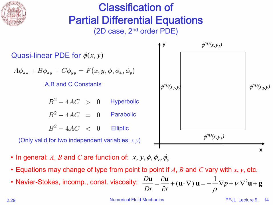
Classification of
Partial Differential Equations(2D case, 2nd order PDE)
y
x
f(n)(x,y2)
f(n)(x,y1)
f(n)(x1,y) f(n)(x2,y)
Quasi-linear PDE for
A,B and C Constants
Hyperbolic
Parabolic
Elliptic
• In general: A, B and C are function of:
• Equations may change of type from point to point if A, B and C vary with x, y, etc.
• Navier-Stokes, incomp., const. viscosity:
, , , ,x yx y f f f
21( )D pDt t
u uu u u g
(Only valid for two independent variables: x,y)
( , )x yf
PFJL Lecture 9, 15Numerical Fluid Mechanics2.29
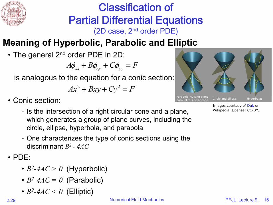
Meaning of Hyperbolic, Parabolic and Elliptic• The general 2nd order PDE in 2D:
is analogous to the equation for a conic section:
• Conic section:- Is the intersection of a right circular cone and a plane,
which generates a group of plane curves, including the circle, ellipse, hyperbola, and parabola
- One characterizes the type of conic sections using the discriminant B2 - 4AC
• PDE:• B2-4AC > 0 (Hyperbolic)
• B2-4AC = 0 (Parabolic)
• B2-4AC < 0 (Elliptic)
Classification of
Partial Differential Equations(2D case, 2nd order PDE)
xx xy yyA B C Ff f f
2 2Ax Bxy Cy F
Images courtesy of Duk onWikipedia. License: CC-BY.
PFJL Lecture 9, 16Numerical Fluid Mechanics2.29
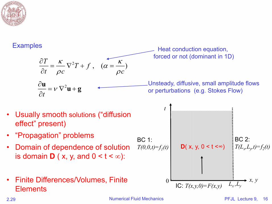
Heat conduction equation, forced or not (dominant in 1D)
Examples
• Usually smooth solutions (“diffusion effect” present)
• “Propagation” problems• Domain of dependence of solution
is domain D ( x, y, and 0 < t < ∞):
• Finite Differences/Volumes, Finite Elements
Unsteady, diffusive, small amplitude flows or perturbations (e.g. Stokes Flow)
2
t
u u g
t
x, y
BC 2:T(Lx,Ly,t)=f2(t)
BC 1:T(0,0,t)=f1(t) D( x, y, 0 < t <∞)
IC: T(x,y,0)=F(x,y)0 Lx ,Ly
2 , ( )T T ft c c
PFJL Lecture 9, 17Numerical Fluid Mechanics2.29
Partial Differential Equations
Parabolic PDE - Example
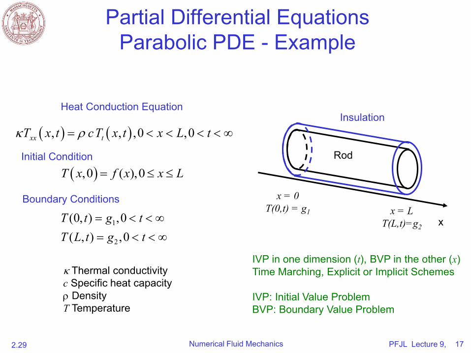
Insulation
Rod
xx = L
T(L,t)=g2
x = 0T(0,t) = g1
Heat Conduction Equation
Thermal conductivityc Specific heat capacity DensityT Temperature
Initial Condition
Boundary Conditions
IVP in one dimension (t), BVP in the other (x)Time Marching, Explicit or Implicit Schemes
IVP: Initial Value ProblemBVP: Boundary Value Problem
( ) ( ), , ,0 ,0xx tT x t cT x t x L t
( ),0 ( ),0T x f x x L
1
2
(0, ) ,0( , ) ,0
T t g tT L t g t
PFJL Lecture 9, 18Numerical Fluid Mechanics2.29
Partial Differential Equations
Parabolic PDE - Example
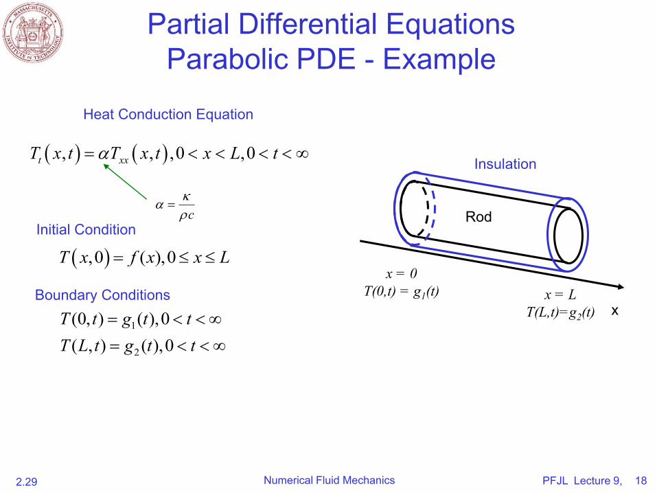
Heat Conduction Equation
Boundary Conditions
Initial Condition
Insulation
Rod
xx = L
T(L,t)=g2(t)
x = 0T(0,t) = g1(t)
s
( ) ( ), , ,0 ,0t xxT x t T x t x L t
c
( ),0 ( ),0T x f x x L
1
2
(0, ) ( ),0( , ) ( ),0
T t g t tT L t g t t
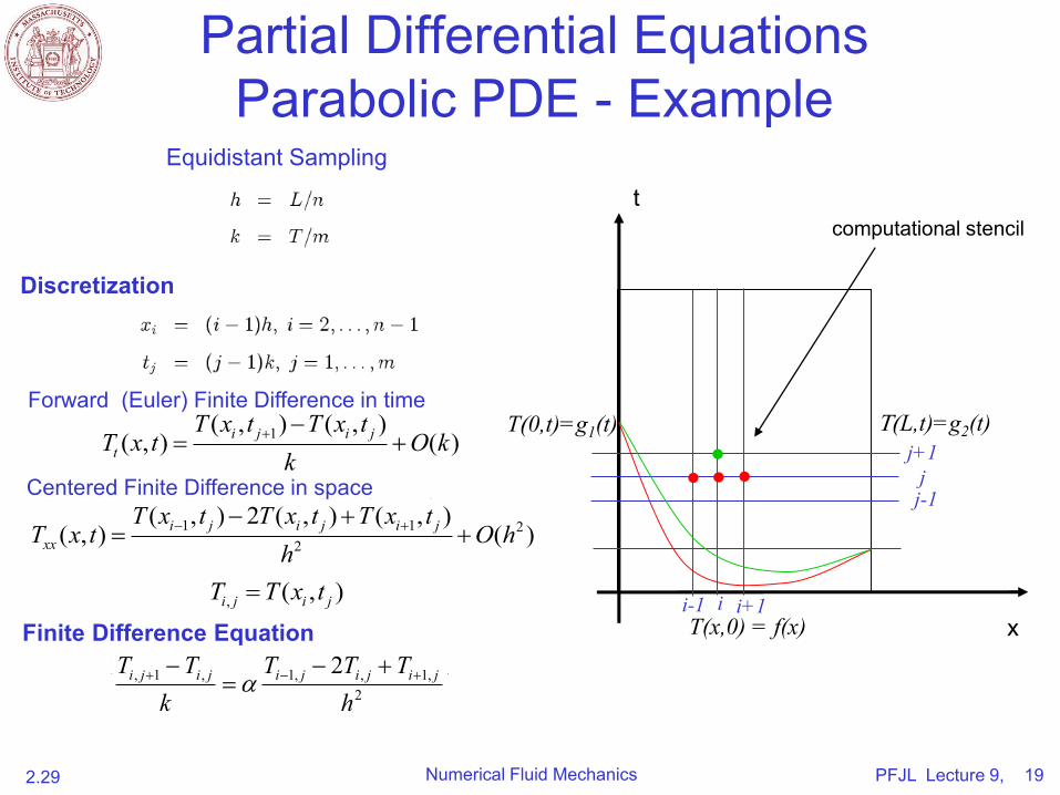
PFJL Lecture 9, 19Numerical Fluid Mechanics2.29
Partial Differential Equations
Parabolic PDE - Example
t
xT(x,0) = f(x)
T(0,t)=g1(t) T(L,t)=g2(t)j+1
j-1j
ii-1 i+1
Equidistant Sampling
Discretization
Finite Difference Equation
1( , ) ( , )( , ) ( )i j i j
t
T x t T x tT x t O k
k
1 1 22
( , ) 2 ( , ) ( , )( , ) ( )i j i j i j
xx
T x t T x t T x tT x t O h
h
, ( , )i j i jT T x t
, 1 , 1, , 1,2
2i j i j i j i j i jT T T T Tk h
Centered Finite Difference in space
Forward (Euler) Finite Difference in time
computational stencil
PFJL Lecture 9, 20Numerical Fluid Mechanics2.29
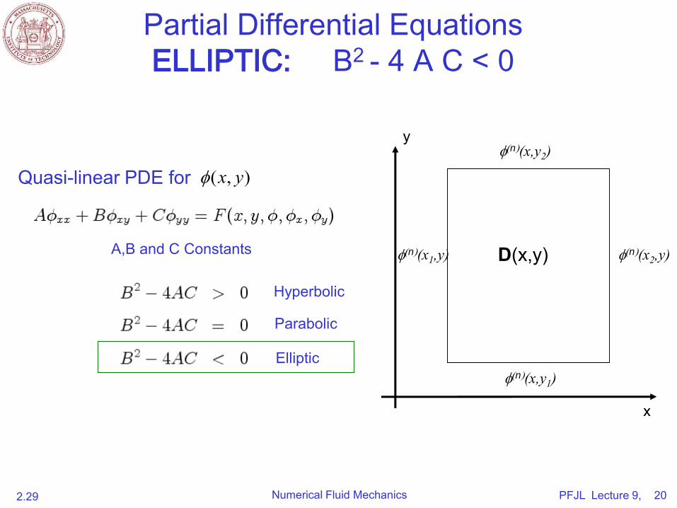
Partial Differential Equations
ELLIPTIC: B2 - 4 A C < 0
y
x
f(n)(x,y2)
f(n)(x,y1)
f(n)(x1,y) f(n)(x2,y)A,B and C Constants
Hyperbolic
Parabolic
Elliptic
D(x,y)
( , )x yfQuasi-linear PDE for
PFJL Lecture 9, 21Numerical Fluid Mechanics2.29
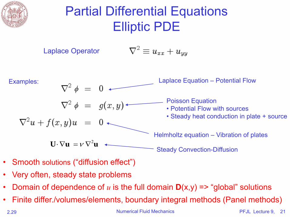
Partial Differential Equations
Elliptic PDE
Laplace Operator
Laplace Equation – Potential Flow
Helmholtz equation – Vibration of plates
Poisson Equation• Potential Flow with sources• Steady heat conduction in plate + source
Examples:
2 U u uSteady Convection-Diffusion
• Smooth solutions (“diffusion effect”) • Very often, steady state problems• Domain of dependence of u is the full domain D(x,y) => “global” solutions• Finite differ./volumes/elements, boundary integral methods (Panel methods)
ϕ
ϕ
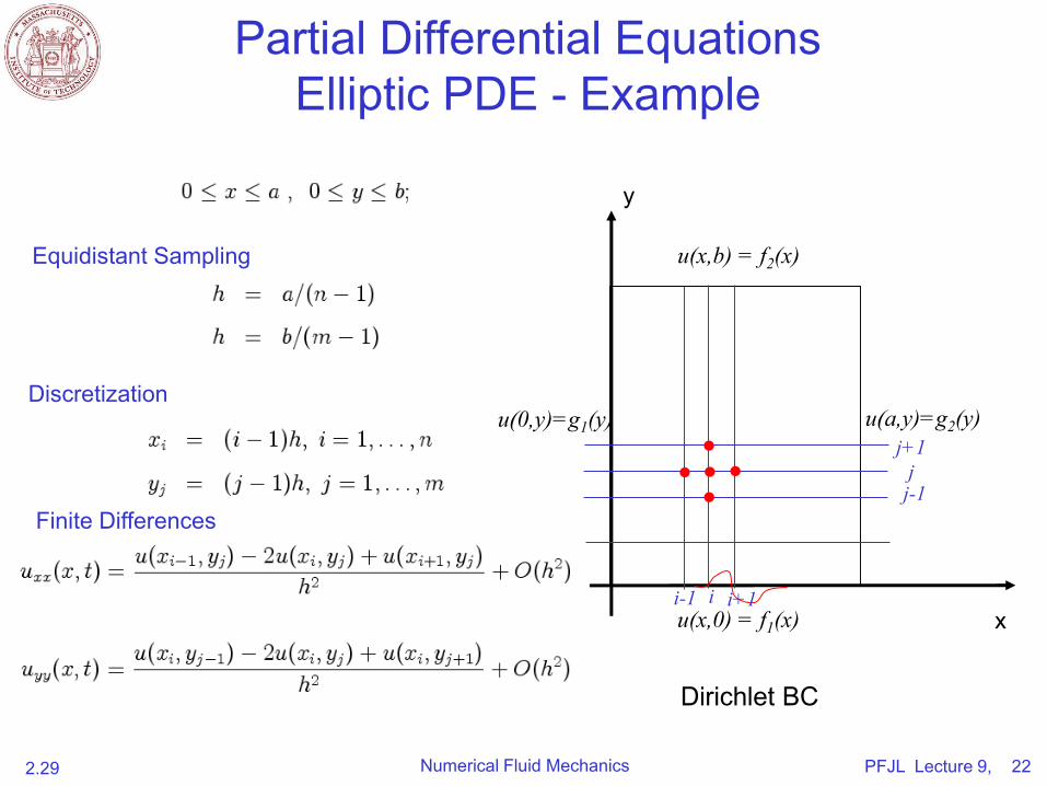
PFJL Lecture 9, 22Numerical Fluid Mechanics2.29
Partial Differential Equations
Elliptic PDE - Example
y
xu(x,0) = f1(x)
u(0,y)=g1(y) u(a,y)=g2(y)j+1
j-1j
ii-1 i+1
Equidistant Sampling
Discretization
Finite Differences
u(x,b) = f2(x)
Dirichlet BC
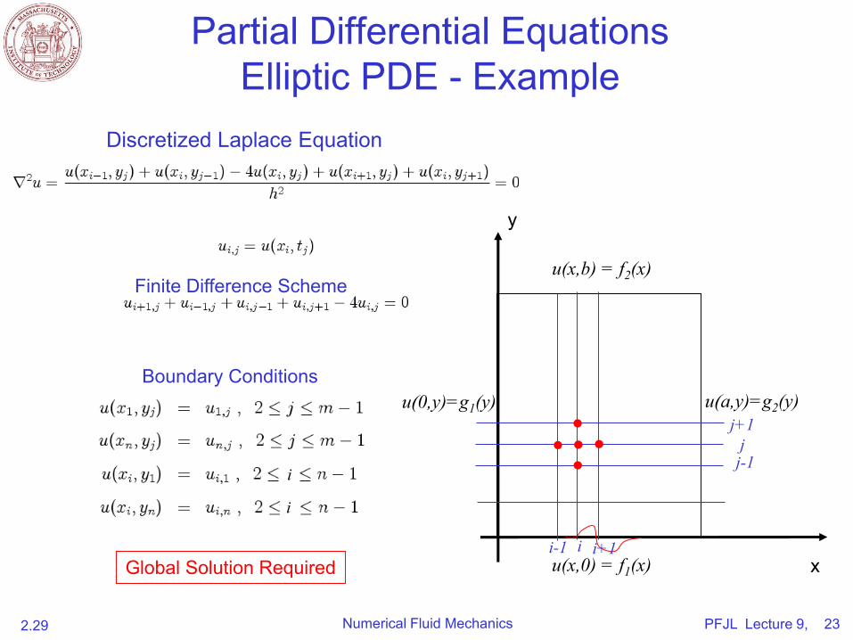
PFJL Lecture 9, 23Numerical Fluid Mechanics2.29
Discretized Laplace Equation
Partial Differential Equations
Elliptic PDE - Example
y
xu(x,0) = f1(x)
u(a,y)=g2(y)j+1
j-1j
ii-1 i+1
u(x,b) = f2(x)Finite Difference Scheme
Global Solution Required
Boundary Conditionsu(0,y)=g1(y)
i
i
MIT OpenCourseWarehttp://ocw.mit.edu
2.29 Numerical Fluid MechanicsSpring 2015
For information about citing these materials or our Terms of Use, visit: http://ocw.mit.edu/terms.