numerical uncertainty analysis for computational fluid dynamics
TRANSCRIPT

Numerical Uncertainty Analysis for Computational Fluid Dynamics using Student T Distribution- Application of CFD Uncertainty Analysis compared to Exact Analytical Solution
Curtis E. Groves 1 and Marcelllie, Ph.D.2
University of Central Florida, Orlando, FL 32816
Paul A. Schallhorn, Ph. 0 .3
National Aeronautics and Space Administration, Kennedy Space Center, FL, 32899
Extended Abstract
Computational Fluid Dynamics (CFD) is the standard numerical tool used by Fluid
Dynamists to estimate solutions to many problems in academia, government, and industry.
CFD is known to have errors and uncertainties and there is no universally adopted method
to estimate such quantities. This paper describes an approach to estimate CFD uncertainties
strictly numerically using inputs and the Student-T distribution. The approach is compared
to an exact analytical solution of fully developed, laminar flow between infinite, stationary
plates. It is shown that treating all CFD input parameters as oscillatory uncertainty terms
coupled with the Student-T distribution can encompass the exact solution.
Nomenclature
a = channel width
f>o = experimental error
= input error
f>model = modeling error
f>num = numerical error
f>s = simulated error
D = experimental value
dp/dx = pressure gradient
=solution changes medium to fine grid
1 Fluids Analysts, NASA Launch Services Program, V A-H3 & PhD Candidate, Department of Mechanical, Materials & Aerospace Engineering, University of Central Florida, AIAA Member. 2 Assistant Professor, Department of Mechanical, Materials & Aerospace Engineering, AlAA Member 3 Environments and Launch Approval Branch Chief, NASA Launch Services Program, VA-H3, and AIAA Member.
https://ntrs.nasa.gov/search.jsp?R=20130014320 2018-02-12T16:50:13+00:00Z

f32 = solution changes coarse to medium grid
ea 21 =extrapolated error
E = comparison error
21 GCI ftne =grid convergence index
h = representative grid size
p =observed order
Rk = convergence parameter
rz1 = ratio of grid sizes between grid 1 and 2
r32 = ratio of grid sizes between grid 3 and 2
S simulated result
Skl solution variable for fme grid
Skz solution variable for medium grid
Sk3 solution variable for coarse grid
Sext 21 = extrapolated solution variable
SL lowest solution variable
Su highest solution variable
Uoscillatory =uncertainty for oscillatory portion of the solution
Umonotonlc =uncertainty for monotonic portion of the solution
Uinput = input uncertainty
u0 = experimental uncertainty
Unwn = numerical uncertainty
UvaJ = validation uncertainty
J1 = viscosity
I. Introduction c FD in many problems is the optimum balance between cost and accuracy. However, a comprehensive approach
for verification using test data is needed for full validation. With shrinking budgets in all areas of aerospace
industry, CFD is commonly used without proper verification and validation. This paper couples traditional

uncertainty analysis with the Student-T distribution to estimate a numerical uncertainty without using test data. The
results are compared to the exact analytical solution of fully developed, laminar flow between infinite, stationary
plates.
A thorough literature review was performed by the authors in AIAA-2013-02581 and it was determined that the
current state of the art for CFD uncertainty analysis is the ASME Standard for Verification and Validation in
Computational Fluid Dynamics and Heat Transfer 2. The standard outlines a validation approach using experimental
errors, modeling assumptions, simulation inputs, and numerical solutions of equations. The error, E, and validation
standard uncertainty Uvah can be defmed and conclusions drawn about whether the model is properly verified. This
paper outlines a method to estimate the numerical uncertainty without using test data and shows the differences
between the proposed methodology and the ASME Standard.
II. Methodology of ASME V & V 20-2009
A schematic showing the nomenclature and an overview of the validation process is shown in Figure 12. The left
side of the figure describes the terminology and the right side describes the validation process .
.§imulation solution value
Experimental .l!ata value
Irue (but unknown value)
Validation point
Reynolds Number, Re
Experimental data, D Comparison error.
E• S-0 validation uncertlintv.
"val
Figure I: Schematic of nomenclature and Overview of Validation Process2
Simulation re1ult, S
The methodology is as follows. The validation comparison error, E, is the difference between the simulated
result, S, and the experimental value, D 2. The goal is to characterize the interval modeling error, Omodel· The
coverage factor, k, used to provide a given degree of confidence (ie 90% assuming a uniform distribution, k=I.65f

The standard also outlines procedures to calculate numerical uncertainty, Unwn, the uncertainty in the simulated result
from input parameters, Uinput. and the experimental uncertainty, u0 2
.
(1)
E=S-D (2)
(3)
Unum is calculated using a Richardson' s Extrapolation approach and defmed as a five-step procedure2•
Step 1, calculate representative grid size, has shown in equation 4.
1
( Total Volume )3
h1 = total number of cells in fine grid
1
( Total Volume )3
h = 2 total number of cells in medium grid
1
h = ( Total Volume )3 3 total number of cells in coarse grid
(4)
Step 2 is to select three significantly (r> 1.3) grid sizes and computer the ratio as shown in equation 52•
(5)
Step 3 is to calculate the observed order, p, as shown in equation 62• This equation must be solved iteratively.
E21 = Sk2 - Ski
E32 = Sk3 - Sk2
(6)
Step 4 is to calculate the extrapolated values as shown in equation 72•
(7)
Step 5 is to calculate the fme grid convergence index and numerical uncertainty as shown in equation 82• This
approached used a factor of safety of 1.25 and assumed that the distribution is Gaussian about the fme grid, 90 %
confidence.

21 1.25 * ea 21 GC/fine =
Cr21P- 1)
GCltin/1 Unum=
1.65
Uinput is calculated using a Taylor Series expansion in parameter space2.
(8)
(9)
U0 is calculated using test uncertainty methodology as defied in the standard2. The purpose of this paper is to
show an estimate of numerical uncertainty without test data. The reader is referred to the ASME standard for further
information.
III. Proposed Methodology without Test Data
Convergence studies require a minimum of three solutions to evaluate convergence with respect to an input
parameter 3. Consider the situation for 3 solutions corresponding to fine Sk), medium Sk2, and coarse Sk3 values for
the kth input parameter 3• Solution changes £ for medium-fine and coarse-medium solutions and their ratio Rk are
defmed by 3:
£21 = Sk2 - Sk1
£32 = Sk3 - Sk2
Rk = £211 £32 (10)
Three convergence conditions are possible3:
(i) Monotonic convergence: 0< Rk < I
(ii) Oscillatory convergence: Rk < 0;
(iii) Divergence: Rk> 1 (11)
The methodology outlined in ASME V&V-20092 assumes monotonic convergence criteria for Unum· Further
increasing the grid does not always provide a monotonically increasing result. This is shown in AIAA-2013-0258 1•
The proposed methodology is to treat all input parameters including the grid as an oscillatory convergence study.
The uncertainty for cells with oscillatory convergence, using the following method outlined by Stem, Wilson,
Coleman, and Paterson 3, can be calculated as follows in equation 12. Sis the simulated result. For this case it is
the upper velocity Suand the lower velocity SL.

(12)
The proposed methodology as compared to the ASME Standard is as follows. If there is no experimental data,
D=O, oo=O, and uo=O.
E=S-D=S
os = S- T
E = S- D = T + os - (T + ov) = os - ov = os
(13)
Report the simulated result, S as S ~Uval (14)
Also instead of assuming a gauss-normal distribution as in the standard when including test data, the k-value will
come from the Student-T distribution as shown in Table 1.
Table 1 - Student - T Distribution, k Values
Number of Cases Degrees of Freedom Confidence 90%
2 I 6.314 3 2 2.92 4 3 2.353 5 4 2.132 6 5 2.015 7 6 1.943 8 7 1.895 9 8 1.86 10 9 1.833 11 10 1.812 12 11 1.796 13 12 1.782 14 13 1.771 IS 14 1.761 16 15 1.753 17 16 1.746 18 17 1.74 19 18 1.734 20 19 1.729 21 20 1.725 22 21 1.721 23 22 1.717 24 23 1.714 25 24 1.711 26 25 1.708 27 26 1.706 28 27 1.703 29 28 1.701 30 29 1.699 31 30 1.697 41 40 1.684 51 50 1.676 61 60 1.671 81 80 1.664 101 100 1.66 121 120 1.658
infty infty 1.645

IV. Fully Developed Laminar Flow Between Stationary Parallel Plates
Fully developed laminar flow between stationary, parallel plates is an exact solution to the Navier-Stokes
Equations as derived in "Introduction to Fluid Mechanics" 4• The width of the channel is (a).
(14)
A CFD model of this problem was created in FLUENT. The fluid is air. Table 2 outlines the parameters
used.
Table 2 -Parameters
a(m) 0.1
rho (kg/m3) 1.225
mu (Ns/m2) 0.00001789
dpjdx (N/m3) -0.000400
The exact solution is shown in Figure I.
Exact
Vtlodty ("'/s)
Figure 1 - Exact Solution

A CFD model was created for the same conditions and the uncertainty calculation performed as outlined in
the next section.
V. Uncertainty Calculation
The uncertainty can be calculated by expanding equation 13 for pressure, density, numerical (grid), and solver.
Uval =
av 82 + av 8 2 + ( (( )2 ) ( )2 ) apressure pressure (;;;:;;;; rho
uV B2 + av B2 + (( ~ )2 ) ( 2 ) anum num ( asolver) solver
+ av B2 . 2 )
1
/z ( (avelocity) velocity) (15)
The proposed method is to calculate the uncertainty as an oscillatory input parameter and multiply by the
appropriate Student-T k-factor.
For Numerical, three grids were used and the t value of2.92.
(16)
(17)
The centerline velocity was chosen as an example to plot, however at all points the uncertainty bands always
encompass the exact solution.

--------- --·---- --- - -- -- ---- ---- --- -
! ! l •
Centerline Velocity vs Exact Solution 0.06 r---------- -- - ---- - -
o.oss
O.OS
I ' O.Cl4S I I
0.04 0.02188
---------
0.0279 0.02792 0.02794
Yelodty (M/s)
--------
-----·---
0.02796 0.02798 0.028
Figure 2- Exact Solution vs. CFD with Uncertainty (Centerline Velocity)- Grid
-cfDMtd
~FDcoarse
Ifthere is also a variation in the inlet velocity due to a tolerance or known bias, run the model at the low and high
limits and use a newt-value of2.132, which corresponds to five cases. The five cases would be three for grids and
two for flow rates. A five percent variation in inlet velocity was chosen for this example.
l
I I ! I
' I I J
= 2 132 * ~ B2 + ov B2 . ( (
2 ) ( 2 ))
1
/z Uva! · (anum) num (ovelocity) veloctty (18)
o.os
0 .04S
0.04
Centerline Velocity vs Exact Solution
r------
~----~--L ._ ____ --+
I ~-j
0.02S 0 .027 0.021
Velocity (M/s)
-------
0.029 0.03 0.031
<:focoarse
~ncert_low
- Uncert_hl&h
_,Dfint
-=f DMtd
~fDcoarse
(19)
l I I
I
-,nlet Velocity Low
0.032 -,nlet Velocity Hlp
- J
Figure 3- Exact Solution vs. CFD with Uncertainty (Centerline Velocity)- Grid and Inlet Velocity

Also to include the outlet pressure boundary condition, run the model at the low and high known bias or tolerances
and use a newt-value of 1.943, which corresponds to seven cases. The seven cases would be three for grid, two for
flow rate, and two for pressure outlet boundary condition.
( ( 2 ) ( 2 ) ( 2 ))liz 1 943 (~) B 2 + ( av ) B2 . + ( av ) B2 Uval = · * anum num ovelocity velocity opressure pressure (20)
(21)
0.06
O.OS~
j
I r---
l i o.os L-----.. I
I O.~S 0--
l .L ____ o_o_:zs_
Centerline Velocity vs Exact Solution
- +-
0.026 0.027 o.ou 0.029
Velocity (m/sJ
0.03
CfOco.rse
~nc:•n_low
- Unc:•n_IIISII
-cFO flno
~0-
~Dcoatse
-.nlet Veloclry Low
0.031 - Inlet V•lodry Hllll
Figure 4- Exact Solution vs. CFD with Uncertainty (Centerline Velocity)- Grid, Inlet Velocity, and Outlet
Pressure
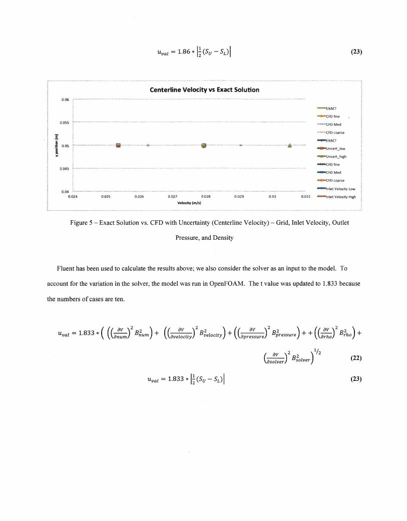
To account for the variation in fluid properties, the kinematic viscosity for air between 0 and 100 degrees Celsius is
13.6X10⁻⁶ to 23.06X10⁻⁶. The model was run at these limits to account for the possible variation in fluid properties
and a new value oft= 1.86 was chosen, which corresponds to the nine cases.
( ( 2 ) ( 2 ) ( 2 ) ( 2 ))liz 1 86 ( av ) 82 + ( av ) 82 . + ( av ) 8 2 + + (~) 8 2 Uval = · * "num num velocity pressure rho v ovelocity opressure orho
_)
(22)
:! I l •
0.()6
I
0.055 ~--I
0.05
0.045 ~-----
0.04 0.024 0 .02S
Centerline Velocity vs Exact Solution
-- -+- -----
0.026 0 .027 0.0211 0.029
Vefoc:ityflll/s)
0.03
(23)
---~,
- EXACT
-cFD~ne
~n<en_low
~ncen_hllh
_,Oflne
-cfD!Md
~FDcoarso
~nlet Velocltv i.Dw
0.031 -,,.let Velocltv Koch
I
I
I i I i I I
Figure 5- Exact Solution vs. CFD with Uncertainty (Centerline Velocity)- Grid, Inlet Velocity, Outlet
Pressure, and Density
Fluent has been used to calculate the results above; we also consider the solver as an input to the model. To
account for the variation in the solver, the model was run in OpenFOAM. The t value was updated to l.S33 because
the numbers of cases are ten.
Uval = 1.833 * ( (( "nouvm )2
Bn2um ) + (( av )
2
Bv2ezoct"ty) + (( oV )
2
Bp2ressure ) + + ((~)
2
Br2ho) + u &velocity &pressure &rho
( &v )2 )1/z
&solver B}olver (22)
(23)

,.---------- ------ - -------
l g .., l ,..
0.06
F o.oss
O.OS I I I
O.IMS r---· l o.oc
0.024 O.o2S
------ --·
Centerline Velocity vs Exact Solution
-- -+-------· - --· --·-·
0 .026 0 .027 0 .02& 0.029 O.Ol 0.011
Veloc:lty (m/s)
~fDIIne
ao (.Oarse
-e-uncen_low
- uncon_hiCh
-cro~~ne
-croMed ~fDooarse
_,nlet Volo<itv Low
_,nlet Veloc:ltv •
-aPtNFOAM
Figure 6 - Exact Solution vs. CFD with Uncertainty (Centerline Velocity) - Grid, Inlet Velocity, Outlet
Pressure, Density, and Solver
Figure 7 is a plot of all the CFD cases, uncertainty, and an exact comparison.
Exact SOlution vs. CFD Uncertainty
O..Gol - ... --·-
0.01 r-
1 t I ' 1 ..
0,02 -·----- -
- -- · .... D.Ol ~
001 O.OB 0112'> 0.0) 0.035
Figure 7 - Exact Solution vs. CFD with Uncertainty (Parallel Plates - Half of Domain)- Grid, Inlet Velocity,
Outlet Pressure, Density, and Solver
VI. Conclusion
It can be concluded that treating all inputs to a CFD model as oscillatory uncertainty parameters coupled with the
Student-T distribution can supply an uncertainty estimate that encompasses the exact solution for the case
considered above (fully developed, laminar, flow between stationary parallel plates). To summarize the approach
and general idea, there is a standard2 for calculating verification and validation of CFD using a combined numerical
and experimental data. The approach described above is a way to estimate the uncertainty of a model if test data is
not available. An analyst should make use of all test data that is available or able to be funded and use the ASME
standard. However, if test data is missing or not attainable, the method described makes assumptions that each CFD
solution belongs to an underlying Student-T distribution and a corresponding uncertainty can be estimated for a
selected confidence interval.
References
[1] Groves, C. , Ilie, M. , Schallhom, Paul. "Comprehensive Approach to Verification and Validation ofCFD
Simulations Applied to Backward Facing Step," AIAA-2013-0258, 2013.
[2] An American National Standard., "Standard for Verification and Validation in Computational Fluid Dynamics and Heat
Transfer", The American Society of Mechanical Engineers. ASME V&V 20-2009.
[3] Stem, F. , Wilson, R. V., Coleman, H. W., and Paterson, E. G., "Verification and Validation of CFD Simulations," Iowa
Institute of Hydraulic Research Report No. 407, September 1999.
[4] Fox, Robert. , McDonald, Alan, "Introduction to Fluid Mechanics" 3rd Edition. John Wiley & Sons, 1985