multiphase flows in cyclone...
TRANSCRIPT
Multiphase Flows in Cyclone Separators Modeling the classification and drying of solid particles using CFD
Master of Science Thesis
Erik A. R. Stendal
Department of Chemical Engineering
Division of Chemical Reaction Engineering
CHALMERS UNIVERSITY OF TECHNOLOGY
Gothenburg, Sweden, 2013

i
Multiphase Flows in Cyclone Separators
Modeling the classification and drying of solid particles using CFD
ERIK A. R. STENDAL
Department of Chemical Engineering
CHALMERS UNIVERSITY OF TECHNOLOGY
Gothenburg, Sweden

ii
Multiphase Flows in Cyclone Separators
Modeling the classification and drying of solid particles using CFD
ERIK A. R. STENDAL
© ERIK A. R. STENDAL, 2013.
Department of Chemical Engineering
Chalmers University of Technology
SE-412 96 Gothenburg
Sweden
Telephone + 46 (0)31-772 1000
Cover:
[Particle tracks for wet Material A particles, colored by diameter,
For more information see Section 4.4.]
[Reproservice]
Gothenburg, Sweden 2013
iii
Multiphase Flows in Cyclone Separators
Modeling the classification and drying of solid particles using CFD
ERIK A. R. STENDAL
Department of Chemical Engineering
Chalmers University of Technology
SUMMARY
This Master’s thesis treats the separation of valuable Material B from invaluable Material A particles
in a cyclone separator. Three desired processes were identified, namely the classification of particles
as well as the drying and pulverization of Material A particles. The cyclone separator is able to
perform all three processes in one step. Using Ansys Fluent both 2D and 3D computational fluid
dynamics simulations was performed to investigate if the computationally cheaper 2D simulations
were able to capture the cyclone separator behavior. The drying process of Material A particles was
modeled using a user-defined function. The simulations were validated against experiments conducted
at a pilot scale.
Three different drying mechanisms for water removal from Material A particles were identified and
investigated. The proposed mechanisms were evaporation from capillaries, centrifugal drying due to
particle spin around its own axis and removal of water during pulverization. It was concluded that all
three mechanisms were possible however the centrifugal drying was considered improbable due to that
the kinetic energy of the particles is lost during pulverization and hence cannot be translated to
rotational energy. The evaporation was modeled for non-pulverized material only.
The 2D axisymmetric simulations showed good agreement with the 3D results for the gas phase and
can hence constitute an attractive alternative to 3D simulations when time is limited. However the 2D
simulations were not able to capture the gas behavior at the nozzles which reflected when examining
the particle tracks. Both in experiments and in simulations it was shown that the particle inlet should
be placed at the barrel side instead of at the barrel roof to achieve a more continuous process with
higher product purity. The classification process modeled in 3D showed excellent agreement with
experiments for Material A particles whereas it was observed that Material B particles accumulated in
various places in the cyclone until particle-particle interaction made the particles come down. It was
seen that evaporation could only explain a fraction of the moisture removal observed during
experiments. The conclusion that the pulverization process is imperative for enhancing the evaporation
rate was drawn.
Keywords: Computational fluid dynamics, CFD, Eulerian-Lagrangian, Discrete phase modeling,
DPM, User-defined function, UDF, Drying of solids.
iv
Acknowledgements This Master’s thesis work has been carried out at XDIN AB and Chalmers University of Technology in
Gothenburg, Sweden during January to June 2013. The work has been supervised by Dr. Mohammad
El-Alti at XDIN AB as well as by Professor Bengt Andersson and Assistant Professor Ronnie Andersson
at Chalmers University of Technology.
First and foremost I would like to thank my three supervisors Dr. Mohammad El-Alti, Professor Bengt
Andersson and Assistant Professor Ronnie Andersson for their invaluable help and guidance
throughout the project.
Thank you also to all members of the Computational Fluid Dynamics department at XDIN AB for
welcoming and helping me when needed.
Last but not least a warm thank you goes out to my family, friends and my better half Sanna for
keeping my spirit and motivational level high.

v
Nomenclature a – Constant used to calculate the drag coefficient
C – Constant or coefficient
d - Diameter
e – Coefficient of restitution
E - Energy
f – Friction factor
F - Force
g – Gravitational acceleration constant
h – Distance between two parallel plates
H - Enthalpy
k – Thermal conductivity or turbulent kinectic energy
l – Pore length
L – Channel length
m - mass
M – Molar mass
n - Integer
P - Pressure
r – Radius or evaporation rate
R – Universal gas constant
S – Source term
t - Time
T - Temperature
u - Velocity
W – Moisture content expressed on a wet basis
x – Specific humidity
y – Wall-distance
Y – Mass fraction
Greek letters
– Constant in source term for energy-dissipation rate
– Dirac function
– Energy-dissipation rate
– Normally distributed random number
– Constant in source term for energy-dissipation rate
- Angle
– Mean free path
– Dynamic viscosity
– Kinematic viscosity
- Density
– Surface
– Time scale or stress
- Scalar
– Angular velocity
vi
Subscripts
ave - Averaged
b - Buoyancy
c – Continuous phase
d – Dispersed phase
D – Drag
e - eddy
eff - Effective
f - Fluid
- Tangential
h – Heat
L - Lagrangian
m - Mass
p - Particle
r - Rotational
T - Turbulent
v - Vaporized
vap - Vaporization
VM – Virtual mass
x – Normal to wall
y – Tangential to wall
Superscripts
´ - Post-impact or fluctuating
‘’ – Fluctuating
+ - Dimensionless
Dimensionless numbers
Kn – Knudsen number
Re – Reynolds number
St – Stokes number
Abbreviations
2D – Two-dimensional
3D – Three-dimensional
CFD – Computational fluid dynamics
RSM – Reynolds stress model
RNG – Re-normalization group
UDF – User-defined function
CAD – Computer-aided design
SDK – Software Development Kit
RANS – Reynolds-Averaged Navier-Stokes
vii
Table of Contents Acknowledgements ................................................................................................................................ iv
Nomenclature .......................................................................................................................................... v
1. Background and introduction ............................................................................................................ 1
1.1 Background to the project ............................................................................................................. 1
1.2 Material properties ....................................................................................................................... 1
1.3 Purpose of the Master’s thesis ...................................................................................................... 2
2. Theory ................................................................................................................................................. 3
2.1 Cyclone separators ........................................................................................................................ 3
2.1.1 The studied cyclone ................................................................................................................ 4
2.2 Particle size distribution ................................................................................................................ 5
2.3 Safety considerations .................................................................................................................... 7
2.4 Drying mechanisms ....................................................................................................................... 7
2.4.1 Drying due to evaporation ..................................................................................................... 7
2.4.2 Drying due to particle spin ................................................................................................... 10
2.4.3 Drying due to particle breakage ........................................................................................... 14
2.4.4 Conclusion about drying mechanisms .................................................................................. 17
2.5 Drying experiments ..................................................................................................................... 17
2.6 Solution procedure ...................................................................................................................... 19
2.7 Discrete phase modeling ............................................................................................................. 20
2.7.1 Forces acting on the particles ............................................................................................... 21
3. Method .............................................................................................................................................. 26
3.1 2D and 3D simulations ................................................................................................................. 26
3.1.1 Geometry and mesh ............................................................................................................. 26
3.1.2 Modeling the vortex breaker cross ...................................................................................... 27
3.1.3 Boundary conditions ............................................................................................................ 28
3.1.4 Discrete phase simulations ................................................................................................... 29
3.3 User-defined function ................................................................................................................. 30
4. Results ............................................................................................................................................... 31
4.1 Comparison between 2D and 3D simulations ............................................................................. 31
4.1.1 Single phase .......................................................................................................................... 31
4.1.2 Multiphase ............................................................................................................................ 32
4.2 Particle inlet placement............................................................................................................... 33
4.3 One-way versus two-way coupling ............................................................................................. 34
viii
4.4 Classification of particles ............................................................................................................. 35
4.5 Drying of particles ....................................................................................................................... 36
5. Conclusions and discussion .............................................................................................................. 37
5.1 Comparison between 2D and 3D ................................................................................................ 37
5.2 Particle inlet placement............................................................................................................... 37
5.3 One-way versus two-way coupling ............................................................................................. 37
5.4 Classification of particles ............................................................................................................. 37
5.5 Drying of particles ....................................................................................................................... 38
6. Future work ....................................................................................................................................... 39
Bibliography .......................................................................................................................................... 40
APPENDIX ................................................................................................................................................. I
A. User defined function ...................................................................................................................... I
B. Modeling drying of solid particles in Fluent ................................................................................... III
B.1 Hooking the UDF to the solver ................................................................................................. III
B.2 Defining the multicomponent injection ................................................................................... III
C. CFD fundamentals ........................................................................................................................... V
C.1 Governing equations ................................................................................................................. V
C.2 Modeling the turbulence ........................................................................................................... V
1
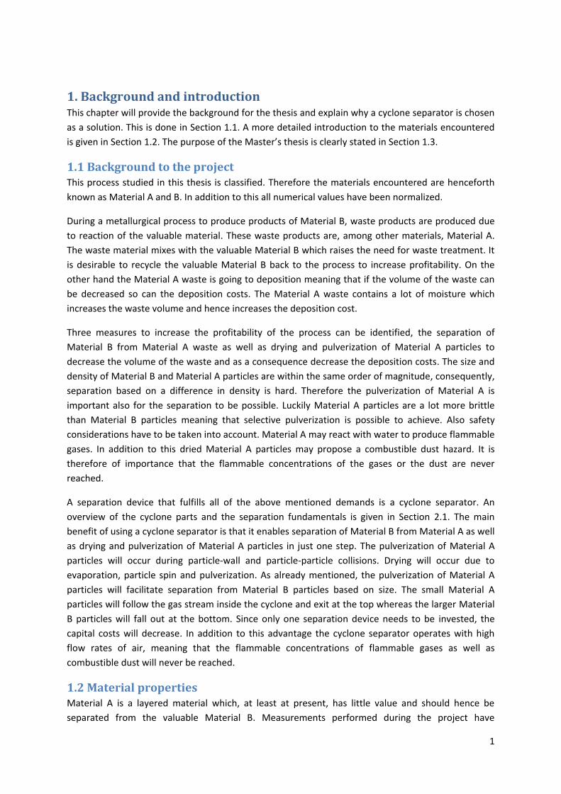
1. Background and introduction This chapter will provide the background for the thesis and explain why a cyclone separator is chosen
as a solution. This is done in Section 1.1. A more detailed introduction to the materials encountered
is given in Section 1.2. The purpose of the Master’s thesis is clearly stated in Section 1.3.
1.1 Background to the project This process studied in this thesis is classified. Therefore the materials encountered are henceforth
known as Material A and B. In addition to this all numerical values have been normalized.
During a metallurgical process to produce products of Material B, waste products are produced due
to reaction of the valuable material. These waste products are, among other materials, Material A.
The waste material mixes with the valuable Material B which raises the need for waste treatment. It
is desirable to recycle the valuable Material B back to the process to increase profitability. On the
other hand the Material A waste is going to deposition meaning that if the volume of the waste can
be decreased so can the deposition costs. The Material A waste contains a lot of moisture which
increases the waste volume and hence increases the deposition cost.
Three measures to increase the profitability of the process can be identified, the separation of
Material B from Material A waste as well as drying and pulverization of Material A particles to
decrease the volume of the waste and as a consequence decrease the deposition costs. The size and
density of Material B and Material A particles are within the same order of magnitude, consequently,
separation based on a difference in density is hard. Therefore the pulverization of Material A is
important also for the separation to be possible. Luckily Material A particles are a lot more brittle
than Material B particles meaning that selective pulverization is possible to achieve. Also safety
considerations have to be taken into account. Material A may react with water to produce flammable
gases. In addition to this dried Material A particles may propose a combustible dust hazard. It is
therefore of importance that the flammable concentrations of the gases or the dust are never
reached.
A separation device that fulfills all of the above mentioned demands is a cyclone separator. An
overview of the cyclone parts and the separation fundamentals is given in Section 2.1. The main
benefit of using a cyclone separator is that it enables separation of Material B from Material A as well
as drying and pulverization of Material A particles in just one step. The pulverization of Material A
particles will occur during particle-wall and particle-particle collisions. Drying will occur due to
evaporation, particle spin and pulverization. As already mentioned, the pulverization of Material A
particles will facilitate separation from Material B particles based on size. The small Material A
particles will follow the gas stream inside the cyclone and exit at the top whereas the larger Material
B particles will fall out at the bottom. Since only one separation device needs to be invested, the
capital costs will decrease. In addition to this advantage the cyclone separator operates with high
flow rates of air, meaning that the flammable concentrations of flammable gases as well as
combustible dust will never be reached.
1.2 Material properties Material A is a layered material which, at least at present, has little value and should hence be
separated from the valuable Material B. Measurements performed during the project have
2
suggested that the density of non-porous Material A is around 85% of that of non-porous Material B
whereas the density of the porous dry Material A particles is around 51% of that of non-porous
Material B. Since the moisture content of the particles is around 36%, on a wet basis, the density of
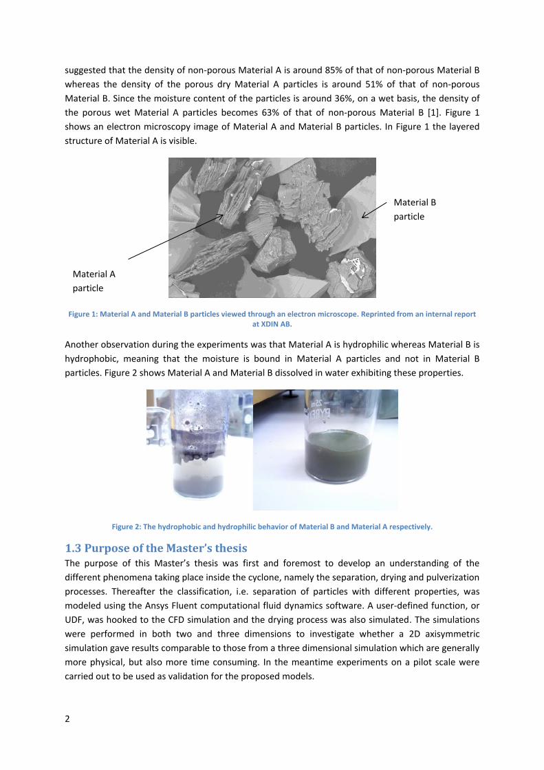
the porous wet Material A particles becomes 63% of that of non-porous Material B [1]. Figure 1
shows an electron microscopy image of Material A and Material B particles. In Figure 1 the layered
structure of Material A is visible.
Figure 1: Material A and Material B particles viewed through an electron microscope. Reprinted from an internal report at XDIN AB.
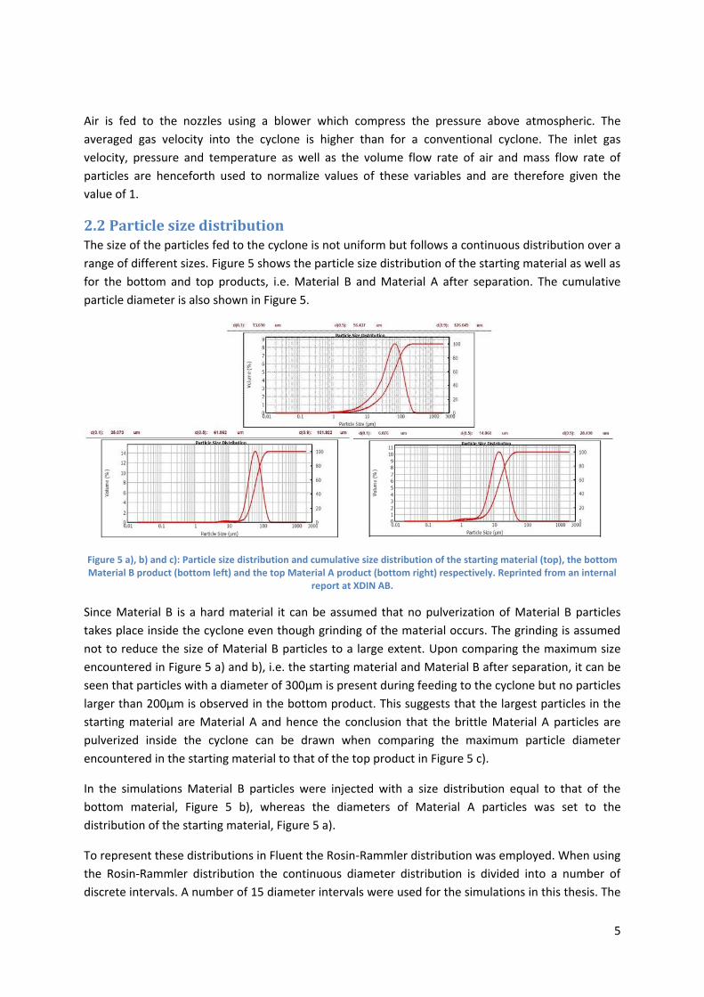
Another observation during the experiments was that Material A is hydrophilic whereas Material B is
hydrophobic, meaning that the moisture is bound in Material A particles and not in Material B
particles. Figure 2 shows Material A and Material B dissolved in water exhibiting these properties.
Figure 2: The hydrophobic and hydrophilic behavior of Material B and Material A respectively.
1.3 Purpose of the Master’s thesis The purpose of this Master’s thesis was first and foremost to develop an understanding of the
different phenomena taking place inside the cyclone, namely the separation, drying and pulverization
processes. Thereafter the classification, i.e. separation of particles with different properties, was
modeled using the Ansys Fluent computational fluid dynamics software. A user-defined function, or
UDF, was hooked to the CFD simulation and the drying process was also simulated. The simulations
were performed in both two and three dimensions to investigate whether a 2D axisymmetric
simulation gave results comparable to those from a three dimensional simulation which are generally
more physical, but also more time consuming. In the meantime experiments on a pilot scale were
carried out to be used as validation for the proposed models.
Material B
particle
Material A
particle

3
2. Theory In Section 2.1, the fundamentals of cyclone separators are discussed. Section 2.2 treats the particle
size distribution. The safety considerations, possible drying mechanisms and the conducted drying
experiments are discussed in Sections 2.3-2.5. Sections 2.6-2.9 cover the governing equations,
solution procedure, turbulence model and discrete phase modeling respectively.
2.1 Cyclone separators The fundamental idea behind a cyclone separator is to separate the particles from the gas by the use
of a centrifugal force. It is also possible to separate particles of different sizes from each other, i.e.
classification. Light particles will not be separated from the gas whereas large particles will. As
mentioned in Section 1.1 it is a classification process that is studied in this thesis. The various parts of
the cyclone are shown in Figure 3.
Figure 3: The various parts of a cyclone separator.
Gas injected at the inlets will first enter the barrel, which is the cylindrical upper part of the cyclone.
When the swirling gas reaches the cone it will be accelerated due to the decreasing cross-sectional
area and a vortex going upwards will form. This vortex will move inside the vortex finder and out
through the gas outlet. The purpose of the vortex finder is to prevent contact between the inner
vortex and the swirling gas in the barrel to prevent large pressure drops. The diameter of the vortex
finder is an important parameter which affects the velocities in the barrel and, as a consequence, the
total pressure drop of the cyclone. Inside the vortex finder a cross-shaped vortex breaker may be
situated. The vortex breaker cross is colored red in Figure 3 and has the purpose of breaking the
rotational motion of the gas. When the rotational gas motion is broken the formation of a low
pressure region is counteracted. The low pressure region may induce reversed flow into the cyclone
through the gas outlet which will lead to large pressure drop and re-entrainment of already
separated particles. The vortex will be able to carry small particles whereas large particles will exit
the cyclone through the dust outlet at the bottom of the cone [2].
The particles injected into the cyclone separator will experience a centrifugal force towards the outer
wall of the cyclone due to the swirling motion of the gas. The centrifugal force will be opposed by the
drag force acting towards the core of the cyclone. Details about the drag force are given in Section
2.9.1. The centrifugal force can be expressed as in Equation (1) [2].

4
(1)
In Equation (1) mp denotes the particle mass, is the tangential velocity and r is the distance from
the cyclone center at which the particle travels. Due to the nature of the centrifugal and the drag
force particles of different size and density will follow different trajectories [2].
2.1.1 The studied cyclone
The cyclone studied in this thesis has eight nozzles. The nozzles are placed at two different heights at
the barrel with four nozzles at each level, as shown in Figure 4.
Figure 4: Placement of the nozzles.
A cross-shaped vortex breaker is placed inside the vortex finder and a cone-shaped vortex breaker is
placed at the dust outlet. The purpose of the cone-shaped vortex breaker is to stabilize the vortex
around the cone tip. The cyclone in the experimental facility had the particle feeding placed at the
barrel roof. During experiments it was observed that particles accumulated at the barrel ceiling
leading to unwanted grinding of Material B particles and hence a lower profitability. A second
problem occurring was batch-wise outflow of particles through the dust outlet. When a large amount
of particles had accumulated a heavy pulse of particles would exit through the dust outlet. It was
observed that the cyclone could run well over a minute between the outflow pulses. Two problems
arise due to the discontinuous outflow, namely that the exiting Material B pulse drags with it large
amounts of Material A and that the discontinuous product flow poses a problem if the cyclone is part
of a larger continuous process. This problem was solved by moving the particle inlet from the barrel
top to the side which led to a more continuous product outflow of higher purity. Simulations
examining the particle inlet placement were run and are presented in Section 4.2. The studied
cyclone is displayed in Figure 3 and the dimensions of the cyclone are summarized in Table 1,
normalized against cyclone diameter.
Table 1: Normlized dimensions of the various parts of the studied cyclone.
Cyclone part Normalized dimension
Cyclone diameter 1 Vortex finder diameter 0.635 Dust outlet diameter 0.317
Barrel height 0.553 Cone height 1.576
Vortex breaker cross height 0.397 Nozzle height 0.238 Nozzle width 0.00238
Vortex breaker cone height 0.159 Vortex breaker
cone diameter 0.232
5
Air is fed to the nozzles using a blower which compress the pressure above atmospheric. The
averaged gas velocity into the cyclone is higher than for a conventional cyclone. The inlet gas
velocity, pressure and temperature as well as the volume flow rate of air and mass flow rate of
particles are henceforth used to normalize values of these variables and are therefore given the
value of 1.
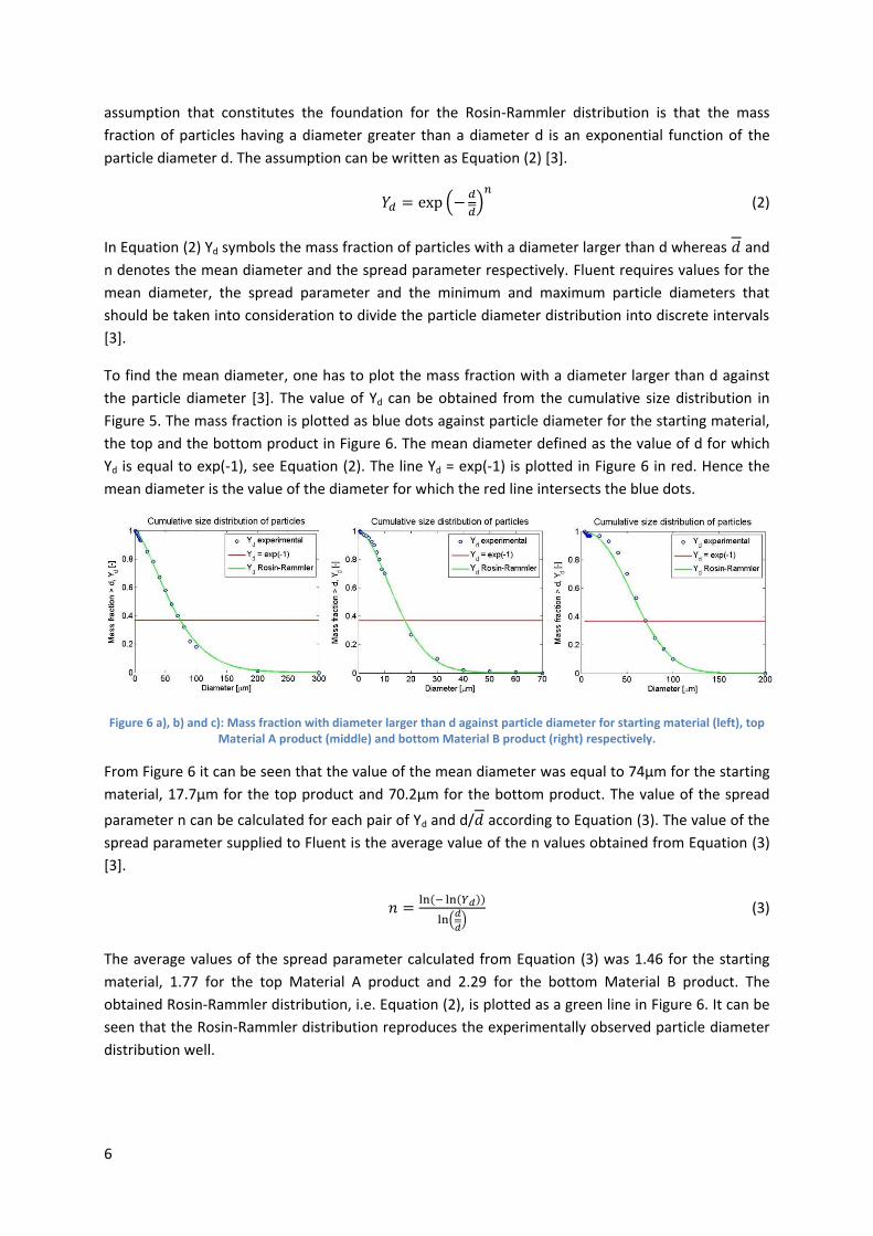
2.2 Particle size distribution The size of the particles fed to the cyclone is not uniform but follows a continuous distribution over a
range of different sizes. Figure 5 shows the particle size distribution of the starting material as well as
for the bottom and top products, i.e. Material B and Material A after separation. The cumulative
particle diameter is also shown in Figure 5.
Figure 5 a), b) and c): Particle size distribution and cumulative size distribution of the starting material (top), the bottom Material B product (bottom left) and the top Material A product (bottom right) respectively. Reprinted from an internal
report at XDIN AB.
Since Material B is a hard material it can be assumed that no pulverization of Material B particles
takes place inside the cyclone even though grinding of the material occurs. The grinding is assumed
not to reduce the size of Material B particles to a large extent. Upon comparing the maximum size
encountered in Figure 5 a) and b), i.e. the starting material and Material B after separation, it can be
seen that particles with a diameter of 300µm is present during feeding to the cyclone but no particles
larger than 200µm is observed in the bottom product. This suggests that the largest particles in the
starting material are Material A and hence the conclusion that the brittle Material A particles are
pulverized inside the cyclone can be drawn when comparing the maximum particle diameter
encountered in the starting material to that of the top product in Figure 5 c).
In the simulations Material B particles were injected with a size distribution equal to that of the
bottom material, Figure 5 b), whereas the diameters of Material A particles was set to the
distribution of the starting material, Figure 5 a).
To represent these distributions in Fluent the Rosin-Rammler distribution was employed. When using
the Rosin-Rammler distribution the continuous diameter distribution is divided into a number of
discrete intervals. A number of 15 diameter intervals were used for the simulations in this thesis. The
6
assumption that constitutes the foundation for the Rosin-Rammler distribution is that the mass
fraction of particles having a diameter greater than a diameter d is an exponential function of the
particle diameter d. The assumption can be written as Equation (2) [3].
(
)
(2)
In Equation (2) Yd symbols the mass fraction of particles with a diameter larger than d whereas and
n denotes the mean diameter and the spread parameter respectively. Fluent requires values for the
mean diameter, the spread parameter and the minimum and maximum particle diameters that
should be taken into consideration to divide the particle diameter distribution into discrete intervals
[3].
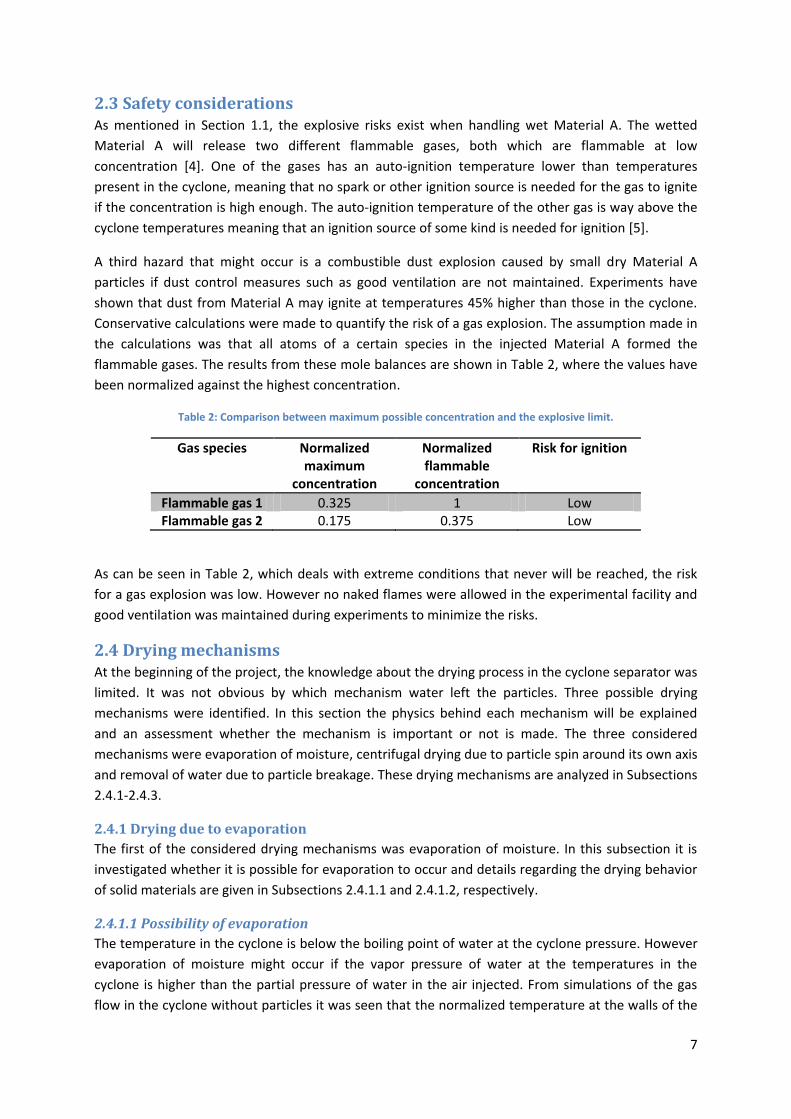
To find the mean diameter, one has to plot the mass fraction with a diameter larger than d against
the particle diameter [3]. The value of Yd can be obtained from the cumulative size distribution in
Figure 5. The mass fraction is plotted as blue dots against particle diameter for the starting material,
the top and the bottom product in Figure 6. The mean diameter defined as the value of d for which
Yd is equal to exp(-1), see Equation (2). The line Yd = exp(-1) is plotted in Figure 6 in red. Hence the
mean diameter is the value of the diameter for which the red line intersects the blue dots.
Figure 6 a), b) and c): Mass fraction with diameter larger than d against particle diameter for starting material (left), top Material A product (middle) and bottom Material B product (right) respectively.
From Figure 6 it can be seen that the value of the mean diameter was equal to 74µm for the starting
material, 17.7µm for the top product and 70.2μm for the bottom product. The value of the spread
parameter n can be calculated for each pair of Yd and d/ according to Equation (3). The value of the
spread parameter supplied to Fluent is the average value of the n values obtained from Equation (3)
[3].
( ( ))
(
)
(3)
The average values of the spread parameter calculated from Equation (3) was 1.46 for the starting
material, 1.77 for the top Material A product and 2.29 for the bottom Material B product. The
obtained Rosin-Rammler distribution, i.e. Equation (2), is plotted as a green line in Figure 6. It can be
seen that the Rosin-Rammler distribution reproduces the experimentally observed particle diameter
distribution well.
7
2.3 Safety considerations As mentioned in Section 1.1, the explosive risks exist when handling wet Material A. The wetted
Material A will release two different flammable gases, both which are flammable at low
concentration [4]. One of the gases has an auto-ignition temperature lower than temperatures
present in the cyclone, meaning that no spark or other ignition source is needed for the gas to ignite
if the concentration is high enough. The auto-ignition temperature of the other gas is way above the
cyclone temperatures meaning that an ignition source of some kind is needed for ignition [5].
A third hazard that might occur is a combustible dust explosion caused by small dry Material A
particles if dust control measures such as good ventilation are not maintained. Experiments have
shown that dust from Material A may ignite at temperatures 45% higher than those in the cyclone.
Conservative calculations were made to quantify the risk of a gas explosion. The assumption made in
the calculations was that all atoms of a certain species in the injected Material A formed the
flammable gases. The results from these mole balances are shown in Table 2, where the values have
been normalized against the highest concentration.
Table 2: Comparison between maximum possible concentration and the explosive limit.
Gas species Normalized maximum
concentration
Normalized flammable
concentration
Risk for ignition
Flammable gas 1 0.325 1 Low Flammable gas 2 0.175 0.375 Low
As can be seen in Table 2, which deals with extreme conditions that never will be reached, the risk
for a gas explosion was low. However no naked flames were allowed in the experimental facility and
good ventilation was maintained during experiments to minimize the risks.
2.4 Drying mechanisms At the beginning of the project, the knowledge about the drying process in the cyclone separator was
limited. It was not obvious by which mechanism water left the particles. Three possible drying
mechanisms were identified. In this section the physics behind each mechanism will be explained
and an assessment whether the mechanism is important or not is made. The three considered
mechanisms were evaporation of moisture, centrifugal drying due to particle spin around its own axis
and removal of water due to particle breakage. These drying mechanisms are analyzed in Subsections
2.4.1-2.4.3.
2.4.1 Drying due to evaporation
The first of the considered drying mechanisms was evaporation of moisture. In this subsection it is
investigated whether it is possible for evaporation to occur and details regarding the drying behavior
of solid materials are given in Subsections 2.4.1.1 and 2.4.1.2, respectively.
2.4.1.1 Possibility of evaporation
The temperature in the cyclone is below the boiling point of water at the cyclone pressure. However
evaporation of moisture might occur if the vapor pressure of water at the temperatures in the
cyclone is higher than the partial pressure of water in the air injected. From simulations of the gas
flow in the cyclone without particles it was seen that the normalized temperature at the walls of the
8
cyclone was around 1. The specific humidity of outdoor air is in the region of 0.5-2% [6]. To check the
validity of the assumption that evaporation was possible the partial pressure of water in air was
calculated. The specific humidity is defined as the ratio of water vapor mass to dry air mass according
to Equation (4) [7].
(4)
The partial pressure of water vapor in air can be expressed as Equation (5) [1].
(5)
Since the specific humidity is expressed on a mass basis it is convenient to rewrite Equation (5) in
terms of mass. Doing this yields the desired partial pressure of water as a function of the specific
humidity shown in Equation (6).
(6)
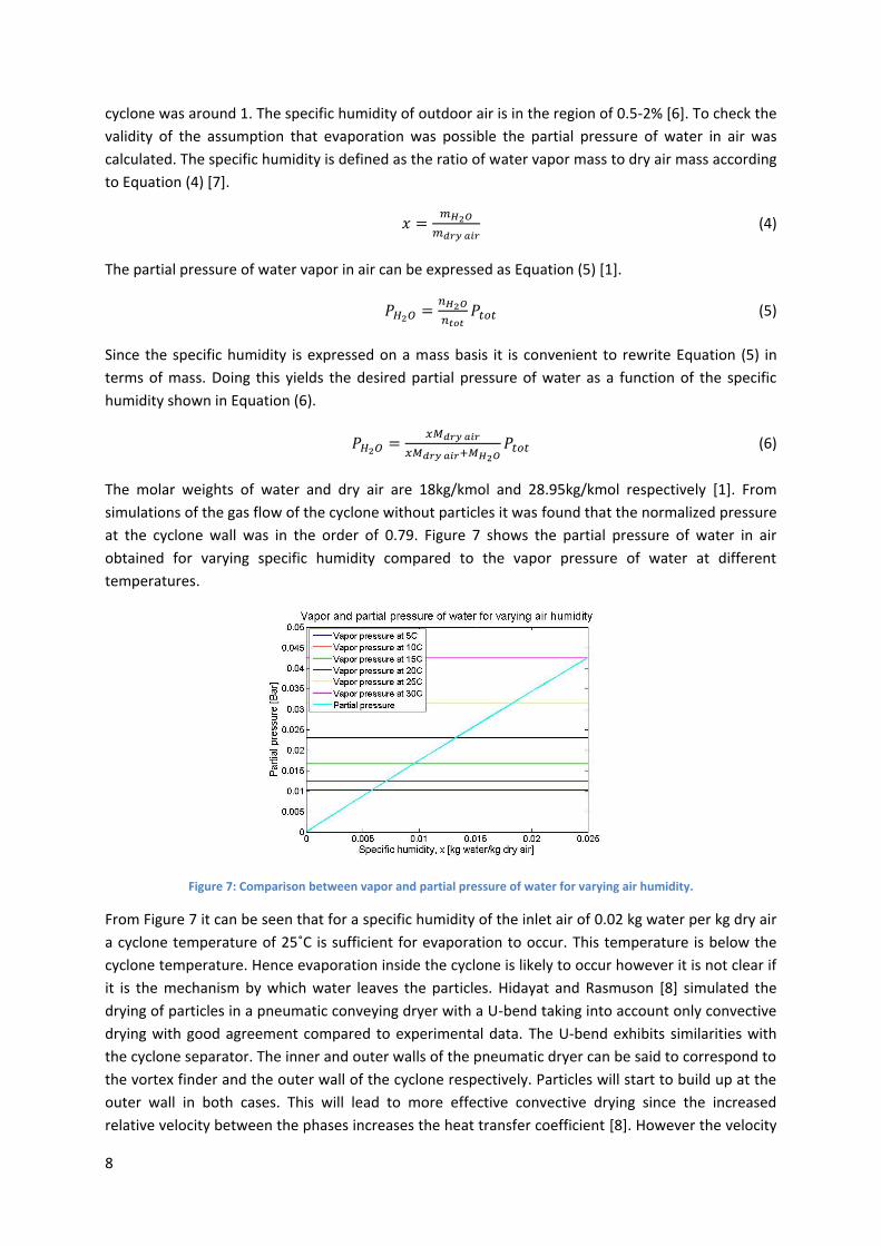
The molar weights of water and dry air are 18kg/kmol and 28.95kg/kmol respectively [1]. From
simulations of the gas flow of the cyclone without particles it was found that the normalized pressure
at the cyclone wall was in the order of 0.79. Figure 7 shows the partial pressure of water in air
obtained for varying specific humidity compared to the vapor pressure of water at different
temperatures.
Figure 7: Comparison between vapor and partial pressure of water for varying air humidity.
From Figure 7 it can be seen that for a specific humidity of the inlet air of 0.02 kg water per kg dry air
a cyclone temperature of 25˚C is sufficient for evaporation to occur. This temperature is below the
cyclone temperature. Hence evaporation inside the cyclone is likely to occur however it is not clear if
it is the mechanism by which water leaves the particles. Hidayat and Rasmuson [8] simulated the
drying of particles in a pneumatic conveying dryer with a U-bend taking into account only convective
drying with good agreement compared to experimental data. The U-bend exhibits similarities with
the cyclone separator. The inner and outer walls of the pneumatic dryer can be said to correspond to
the vortex finder and the outer wall of the cyclone respectively. Particles will start to build up at the
outer wall in both cases. This will lead to more effective convective drying since the increased
relative velocity between the phases increases the heat transfer coefficient [8]. However the velocity

9
in the pneumatic dryer was lower than that in the cyclone so no pulverization of particles increasing
the drying efficiency was observed in the pneumatic dryer.
2.4.1.2 Drying behavior of solids
Wet solids bind moisture in two different ways depending on their properties and are therefore
classified into two categories. The first category contains the granular and crystalline solids. These
solids bind moisture in open pores. Examples of solids of the first category are sand and catalysts.
The second category is occupied by fibrous and gel-like materials. Solids of the second category bind
moisture in fibers or very fine pores and include materials such as wood and cotton [7]. Electron
microscopy pictures, Figure 1, and the molecular structure of Material A reveal that Material A
belongs to the first category.
When solids are dried using gas as a convective medium the moisture content of the solid as a
function of time can be measured. If the obtained curve is differentiated with respect to time the
drying rate is obtained. The drying rate as a function of moisture content is plotted in Figure 8. Three
different drying periods are clearly shown. Figure 8 also displays the moisture content in the particle
during the different drying periods [9].
Figure 8: Drying rate as a function of moisture content. Reprinted from Vaxelaire and Cézac [9].
As can be seen in Figure 8 the drying of solids can be divided into three periods. These periods are,
from high to low moisture content, the pre-heat, the constant-rate and the falling-rate drying period.
In the pre-heat period the solid is covered with moisture and the moisture is heating up to the wet-
bulb temperature. Some moisture is evaporated during this process at an increasing rate. When the
wet-bulb temperature is reached evaporation of the surface moisture will occur at this temperature
at a constant rate until the surface is no longer covered with moisture. During the constant-rate
period the limiting factor is the transport of heat to the surface. When the surface moisture has been
evaporated the drying rate will start to decrease. This is due to the decrease in heat transfer area as
the surface is no longer covered with moisture. During the falling-rate period moisture is evaporated
from capillaries and the limiting factor is transport of moisture to the surface due to capillary action
[7].
Starting from the right in Figure 8, i.e. at high moisture content, the drying rate increases during the
pre-heat period to later become constant during the constant rate period. Two different falling rate
periods can be identified even though this does not always occur. For the second falling rate period
10
the limiting factor is diffusion of gas in the capillaries [7]. Figure 8 also shows how the moisture
distribution in the solid changes during the evaporation process.
During this project drying experiments with particles of Material A were conducted to obtain a
similar curve to that shown in Figure 8. The drying rate as a function of moisture content was critical
for constructing a UDF that was able to correctly describe the drying behavior of the particles. The
drying rate curve for particles of Material A is shown in Section 2.5.
2.4.2 Drying due to particle spin
When a particle spins around its own axis a centrifugal force will be induced. This force will drive
water from the particle center towards the surface, hence enhance evaporation efficiency. However
the centrifugal force will be opposed by the capillary force acting in the opposite direction [10]. The
capillary force is described in Subsection 2.4.2.1. In Subsection 2.4.1.2 the conditions at which drying
due to centrifugation may occur are discussed.
2.4.2.1 Capillary action
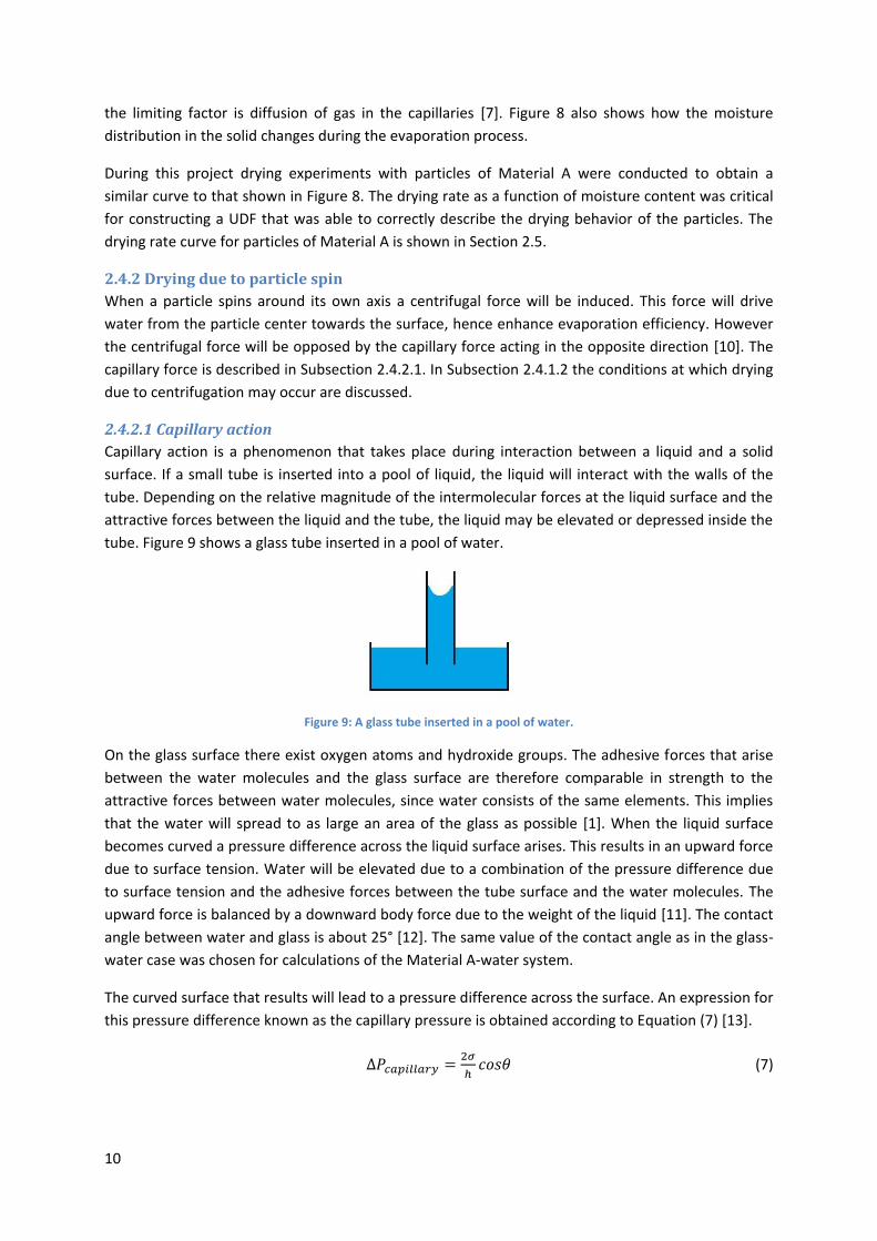
Capillary action is a phenomenon that takes place during interaction between a liquid and a solid
surface. If a small tube is inserted into a pool of liquid, the liquid will interact with the walls of the
tube. Depending on the relative magnitude of the intermolecular forces at the liquid surface and the
attractive forces between the liquid and the tube, the liquid may be elevated or depressed inside the
tube. Figure 9 shows a glass tube inserted in a pool of water.
Figure 9: A glass tube inserted in a pool of water.
On the glass surface there exist oxygen atoms and hydroxide groups. The adhesive forces that arise
between the water molecules and the glass surface are therefore comparable in strength to the
attractive forces between water molecules, since water consists of the same elements. This implies
that the water will spread to as large an area of the glass as possible [1]. When the liquid surface
becomes curved a pressure difference across the liquid surface arises. This results in an upward force
due to surface tension. Water will be elevated due to a combination of the pressure difference due
to surface tension and the adhesive forces between the tube surface and the water molecules. The
upward force is balanced by a downward body force due to the weight of the liquid [11]. The contact
angle between water and glass is about 25° [12]. The same value of the contact angle as in the glass-
water case was chosen for calculations of the Material A-water system.
The curved surface that results will lead to a pressure difference across the surface. An expression for
this pressure difference known as the capillary pressure is obtained according to Equation (7) [13].
(7)
11
In Equation (7) h is the distance between two parallel plates or in this case two Material A layers, is
the contact angle and is the surface tension which can be expressed as Equation (8) for water and
air [11].
( ) (8)
2.4.2.2 Particle spin
When a particle collides with a wall or another particle it might begin to rotate around its own axis.
This rotation will lead to the rise of a centrifugal force that may drive water in the capillaries towards
the surface of the particle. This phenomenon is opposed by the capillary force and hence a
comparison between the magnitude of the centrifugal and the capillary force is necessary to
determine if drying due to centrifugation is possible. The centrifugal pressure can be calculated
according to Equation (9) [14].
(
) (9)
In Equation (9) is the angular velocity of the particle whereas and are the distances from the
particle center between which liquid resides. Garcia-Cordero et al [15] conducted centrifugal
experiments with a rotating disc and microfluidic channels. They state that liquid will be transported
out of the pores by the centrifugal force when the angular velocity is high enough for the centrifugal
pressure to be larger than the capillary force. By putting Equation (7) equal to Equation (9) and
solving for the condition labeled Equation (10) for centrifugal transport to occur is obtained [15].
√
(
) (10)
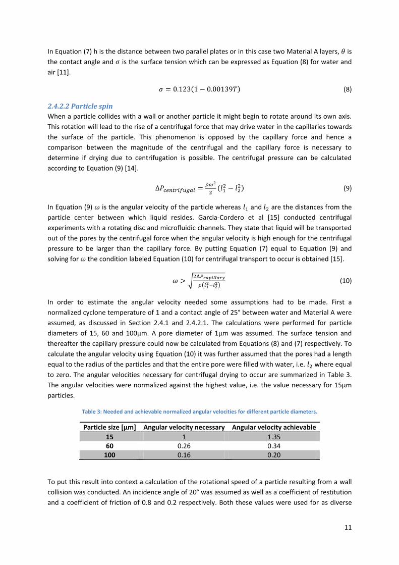
In order to estimate the angular velocity needed some assumptions had to be made. First a
normalized cyclone temperature of 1 and a contact angle of 25° between water and Material A were
assumed, as discussed in Section 2.4.1 and 2.4.2.1. The calculations were performed for particle
diameters of 15, 60 and 100µm. A pore diameter of 1μm was assumed. The surface tension and
thereafter the capillary pressure could now be calculated from Equations (8) and (7) respectively. To
calculate the angular velocity using Equation (10) it was further assumed that the pores had a length
equal to the radius of the particles and that the entire pore were filled with water, i.e. where equal
to zero. The angular velocities necessary for centrifugal drying to occur are summarized in Table 3.
The angular velocities were normalized against the highest value, i.e. the value necessary for 15µm
particles.
Table 3: Needed and achievable normalized angular velocities for different particle diameters.
Particle size [µm] Angular velocity necessary Angular velocity achievable
15 1 1.35 60 0.26 0.34
100 0.16 0.20
To put this result into context a calculation of the rotational speed of a particle resulting from a wall
collision was conducted. An incidence angle of 20° was assumed as well as a coefficient of restitution
and a coefficient of friction of 0.8 and 0.2 respectively. Both these values were used for as diverse
12
materials as aluminum and nylon in the book by Crowe et al and were therefore deemed to give a
reasonable approximation of the corresponding values for Material A [16]. The particle did not have
any rotational speed before the impact. The tangential and normal impact velocities to the wall are
defined as Equation (11 a) and (11 b).
( ) (11 a)
( ) (11 b)
In this case the x-direction is tangential and the y-direction is normal to the wall. The particle will
deform upon impact with the wall to later regain its former shape. Hence the collision can be divided
into two periods, namely the compression and the recovery period. During the collision the particle
slides against the wall. The formulas used to calculate the relation between pre and post impact
properties such as angular velocity depends on whether the particle stops sliding in the compression
or recovery period or continues to slide during both periods. If the condition labeled Equation (12) is
fulfilled the particle slides throughout both periods [16].
( )
| | (12)
In Equation (12) f is the friction factor and e is the coefficient of restitution. Upon inserting the values
given above and by utilizing the expression for given as Equation (11 a), it is clear that this
condition is fulfilled. Hence the angular velocity after impact should be calculated according to
Equation (13) [16].
( ) (13)
The ϵx encountered in Equation (13) is the proportion of the velocity tangential to the wall defined as
ux/u. When Equation (11 a) for the normal velocity and the expression for ϵx are inserted into
Equation (13) and the initial angular velocity is set to zero an expression for the pre-impact velocity
needed for centrifugal transport of water can be obtained [16]. This expression is given as Equation
(14).
( ) ( ) ( ) (14)
Upon inserting the values into Equation (14) it can be seen that a pre-impact normalized velocity in
the order of 0.32 is necessary for all three particle diameters considered. Simulations show that the
particles will hit the wall with a normalized velocity magnitude of 0.41 and hence it is possible for the
particles to obtain the rotational speed that allows for drying of the particles due to centrifugation.
The angular velocity resulting from a collision at a normalized velocity of 0.41 was calculated for all
three particle diameters using Equation (13) and the obtained values were used for all following
calculations. The achievable normalized angular velocities are presented in Table 3. However a
question that remains is whether the particles will bounce or break during a wall collision at such
high velocity. Experimental observations during the Master’s thesis project suggest that the particles
will break rather than bounce and hence rotation after the impact might be at significantly lower
rotational speeds if any. This is because the kinetic energy is lost during the particle breakage and is
not translated to rotational energy.
13
Due to the hydrophilic behavior of Material A it can be suspected that the water removed from the
capillaries due to particle spin will not form a droplet on the particle surface. Instead the water will
spread over the particle surface and hence increase the evaporation rate. An important aspect to
consider is the time needed for friction to reduce the rotation of the particles. The rotational speed
of the particles will eventually reduce below the critical and hence water will no longer be
transported to the particle surface due to the centrifugal force. A tool to assess the time taken to
reduce the rotational speed is the rotational time scale which corresponds to the time needed for
the rotational speed of the particle to be reduced by 63% [17] . The rotational time scale can be
defined from the equation of rotational motion of a particle according to Equation (15) [18].
(15)
The rotational motion of the particles will be damped by viscosity and the difference in drag across
the particle surface. At one side of the particle the relative velocity between the gas and the particle
will be reduced due to the rotation. On this side a torque acting to preserve the rotational motion
arises. On the other side of the particle a torque acting to damp the rotational motion arises. Taken
this into account the torque balance can be expressed as Equation (16) [16].
( )
( )
(16)
The term on the left hand side of Equation (16) is torque accumulation. The terms on the right hand
side represents viscous damping, torque preserving the rotational motion and torque damping the
rotational motion respectively. Since the periphery velocity is defined as the product between the
rotational speed and the particle radius the particle response time can, upon comparing Equation
(15) and (16) and manipulating the expression to contain the particle Reynolds number, be defined
as Equation (17). The particle Reynolds number is defined in Equation (29).
(17)
The particle Reynolds number is easily obtained from simulations meaning that the drag coefficient
can be obtained from Figure 10. Hence the rotational response time can be calculated for particles of
different size. The value of the drag coefficient does not increase with rotational speed for rotating
smooth spheres [16]. However Material A particles are not smooth spheres and hence the drag
coefficient should increase with rotational speed [19].
The rotational response time should be compared to the time it takes for water to be centrifuged out
of the capillary. If the rotational response time is less than the centrifugation time the rotational
motion of the particles will be damped out before the water has left the capillaries. During the
centrifugation a pressure difference arises between the center and the periphery of the particle. Due
to this pressure gradient the water will leave the capillary. The pressure difference due to particle
spin can be calculated according to Equation (9) [14]. Since Material A is a layered material the flow
in the capillaries can be seen as similar to flow between two parallel plates due to a pressure
gradient. Hence the average velocity of the water in the capillary can be calculated according to
Equation (18) [20].
(
) (18)
14
In Equation (18) h is the distance between the plates and L is the channel length. Since the velocity
can be calculated and the channel length is known, the time required for the capillary water to flow a
length equal to that of the capillary can now be calculated. One assumption behind Equation (18) is
that of fully developed flow, i.e. that the fluid has the average velocity from the beginning and hence
no acceleration is needed, meaning that the flow time will in reality be longer due to the acceleration
of the fluid needed to reach the average velocity. Also the above expression is valid for straight
channels which also may not be the case. In reality the capillaries may be irregular leading to a larger
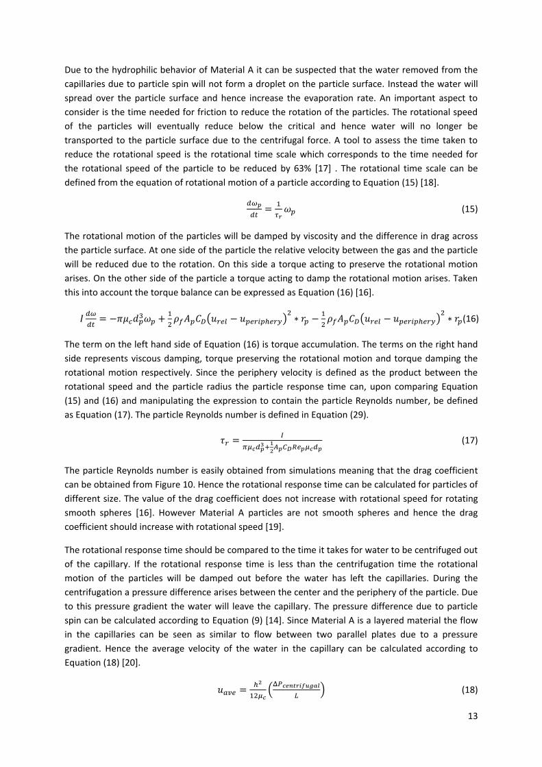
time scale for capillary flow. The normalized rotational time scale and the time required for the liquid
to flow out of the capillary are summarized in Table 4 for the three different particle diameters. The
time scales are normalized against the largest value.
Table 4: Comparison between the normalized rotational and the capillary flow time scales.
Particle diameter [µm] Rotational time scale Capillary flow time scale
15 0.036 2.3e-4 60 0.43 3.4e-3
100 1 9.4e-3
As can be seen from Table 4 the rotational time scale is two orders of magnitude greater than the
time scale for flow out of the capillaries. Hence the water in the capillaries will have time to be
transported to the particle surface before the rotational motion is ended, even though the time scale
should be slightly longer due to the time needed for acceleration. Therefore the conclusion that the
drying efficiency is enhanced by particle spin is drawn. However it is likely that the kinetic energy of
the particles is lost and not translated to rotational motion when the particles break during wall
collisions. Therefore it is suspected that the particle spin contribution to the drying process is
negligible. Particle spin is not included in the simulations.
2.4.3 Drying due to particle breakage
The pulverization of particles favors the drying process in two ways. Firstly the contact area between
the particles and the gas increases which enhances heat and mass transfer and also the internal
transport resistance of the particles will decrease. In addition some water may be released during the
breakage process itself. Particles may break during particle-wall and particle-particle collisions.
Therefore it is important to examine whether these collisions occur or not. An investigation of
particle-wall collisions is provided in Subsection 2.4.3.1 and one of particle-particle interaction in
Subsection 2.4.3.2.
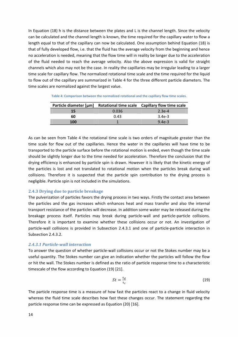
2.4.3.1 Particle-wall interaction
To answer the question of whether particle-wall collisions occur or not the Stokes number may be a
useful quantity. The Stokes number can give an indication whether the particles will follow the flow
or hit the wall. The Stokes number is defined as the ratio of particle response time to a characteristic
timescale of the flow according to Equation (19) [21].
(19)
The particle response time is a measure of how fast the particles react to a change in fluid velocity
whereas the fluid time scale describes how fast these changes occur. The statement regarding the
particle response time can be expressed as Equation (20) [16].
15
( ) (20)
If the equation of motion is written for a particle an expression for the particle response time can be
obtained upon comparison with Equation (20). The equation of motion for a particle, including only
the relevant forces discussed in Section 2.9.1, can be written as Equation (21).
( )
(21)
Upon comparing Equation (21) and (20) it can be seen that the particle response time can be written
as Equation (22).
(22)
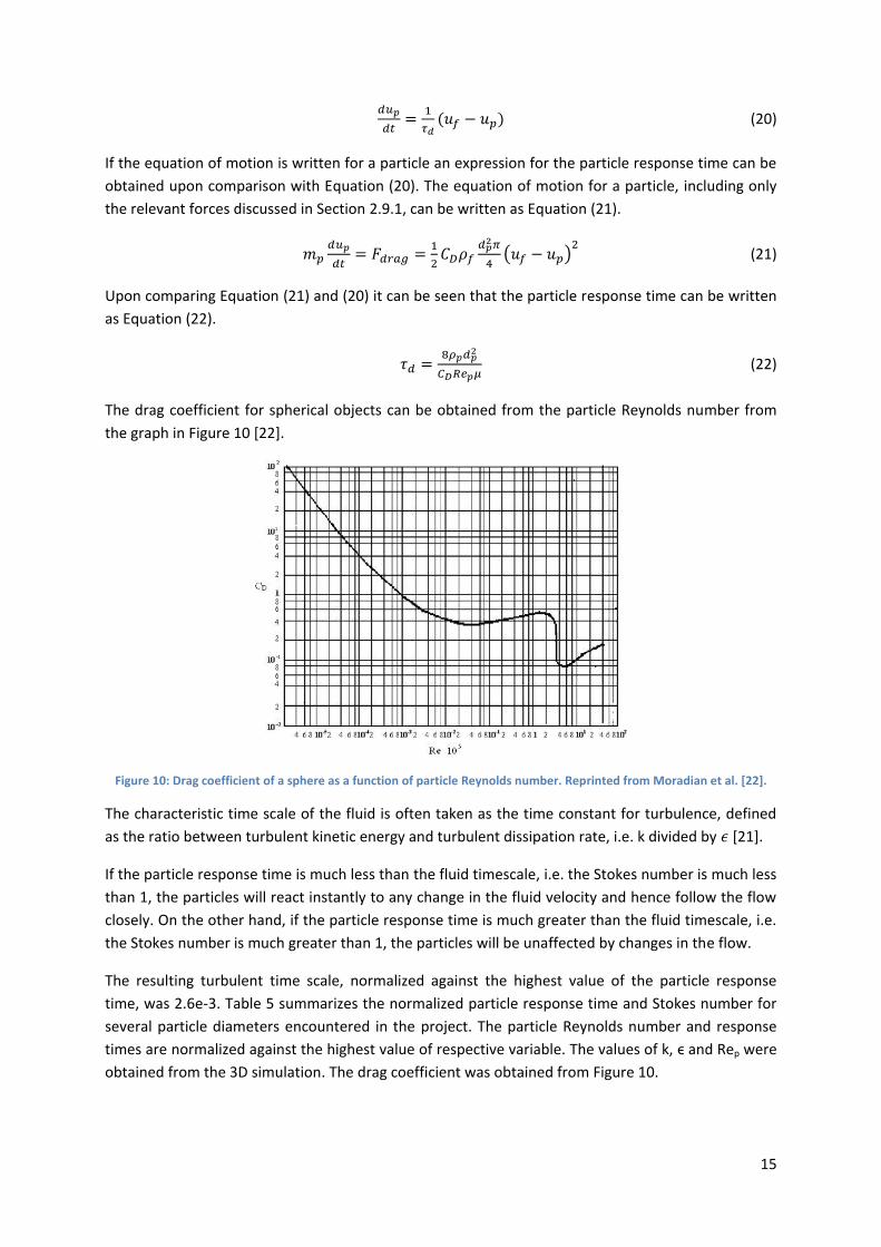
The drag coefficient for spherical objects can be obtained from the particle Reynolds number from
the graph in Figure 10 [22].
Figure 10: Drag coefficient of a sphere as a function of particle Reynolds number. Reprinted from Moradian et al. [22].
The characteristic time scale of the fluid is often taken as the time constant for turbulence, defined
as the ratio between turbulent kinetic energy and turbulent dissipation rate, i.e. k divided by [21].
If the particle response time is much less than the fluid timescale, i.e. the Stokes number is much less
than 1, the particles will react instantly to any change in the fluid velocity and hence follow the flow
closely. On the other hand, if the particle response time is much greater than the fluid timescale, i.e.
the Stokes number is much greater than 1, the particles will be unaffected by changes in the flow.
The resulting turbulent time scale, normalized against the highest value of the particle response
time, was 2.6e-3. Table 5 summarizes the normalized particle response time and Stokes number for
several particle diameters encountered in the project. The particle Reynolds number and response
times are normalized against the highest value of respective variable. The values of k, ϵ and Rep were
obtained from the 3D simulation. The drag coefficient was obtained from Figure 10.

16
Table 5: Stokes number for different particle diameters.
Particle diameter [µm] Rep St
1 0.004 2.1e-4 0.081 15 0.07 0.023 8.85 60 0.26 0.19 72.40
100 0.44 0.29 106.9 300 1 1 393.8
From Table 5 it is clear that the smallest particles will follow the flow closely whereas larger particles
will not be affected by flow variations. This implies that particle-wall collisions will occur for almost
all particles, which is the reason for the pulverization of the brittle Material A. Hence, pulverization of
particles is also a possible drying mechanism.
2.4.3.2 Particle-particle interaction
If the volume fraction of particles exceeds 0.001 particle-particle interaction has to be taken into
account [16]. Particle-particle interaction was not included in the simulations of this thesis due to the
accompanying increase in computational time and the existing time limitation. However to check the
validity of this assumption an estimate of the particle volume fraction was made. Particles were
injected at a volume flow rate normalized against the inlet air flow rate of 2.6e-5 whereas the
volume flow rate of air was 1. Hence the flow should be dilute and particle-particle interactions
should not have to be taken into account. However, as can be seen in Chapter 4, the particles
accumulate at various areas of the cyclone and hence the local volume fraction may be very large.
Since more or less continuous outflow of particles was observed during experiments the conclusion
that particle-particle interactions occur and is one of the reasons for particles leaving the
accumulation zones was drawn. Three phenomena responsible for particles leaving the accumulation
zones can be identified. The first phenomenon is the decrease in particle velocity associated with
wall collisions. When particles collide with the wall some of their tangential velocity is lost which
decreases the magnitude of the centrifugal force, see Equation (1). Hence, the particles will have a
larger tendency to fall down. The second phenomenon is particle-particle collisions. In areas with
high volume fraction collisions will occur frequently which will force particles out of the accumulation
zones. Since the volume fraction of particles is much lower outside of the accumulation zones,
almost no collisions forcing particles into the accumulation zones will occur. The third phenomenon
counteracting particle accumulation is the gas flow from the walls towards the center of the cyclone.
The gas is injected at the walls and hence a continuous flow from the walls towards the center of the
cyclone occurs which drags with it small particles.
The particle-particle collisions and grinding that may occur should increase the pulverization effect
and hence increase the drying efficiency. Although it is suspected that the major part of the
pulverization takes place at the first wall collision after injection.
If the volume fraction of particles is high, the presence of particles will affect the flow. This is known
as two-way momentum coupling. If the volume fraction of the particles is too low to affect the flow
the coupling is said to be one-way [21]. A comparison was made between the results of a one-way
and a two-way momentum coupled simulation. From the comparison it could be seen that two-way
coupling affected the continuous phase at the accumulation zones but not at all in the main part of
17
the cyclone. Therefore only one-way coupling was used for the rest of the simulations. The
comparison is shown in Chapter 4.
2.4.4 Conclusion about drying mechanisms
The calculations and discussion in the above subsections clearly shows that evaporation will take
place in the cyclone separator. When the particles collide with the wall after the inlet and with each
other at the accumulation zones pulverization of Material A will occur. This phenomenon will
enhance the drying efficiency due to an increased contact area between the phases and decreased
internal transport resistance of the particles. Spinning particles are able to transport water out of the
capillaries to the surface which also increases the drying rate. However it is suspected that the kinetic
energy of the particles are lost when the particles hit the wall and breaks rather than being
translated into rotational energy.
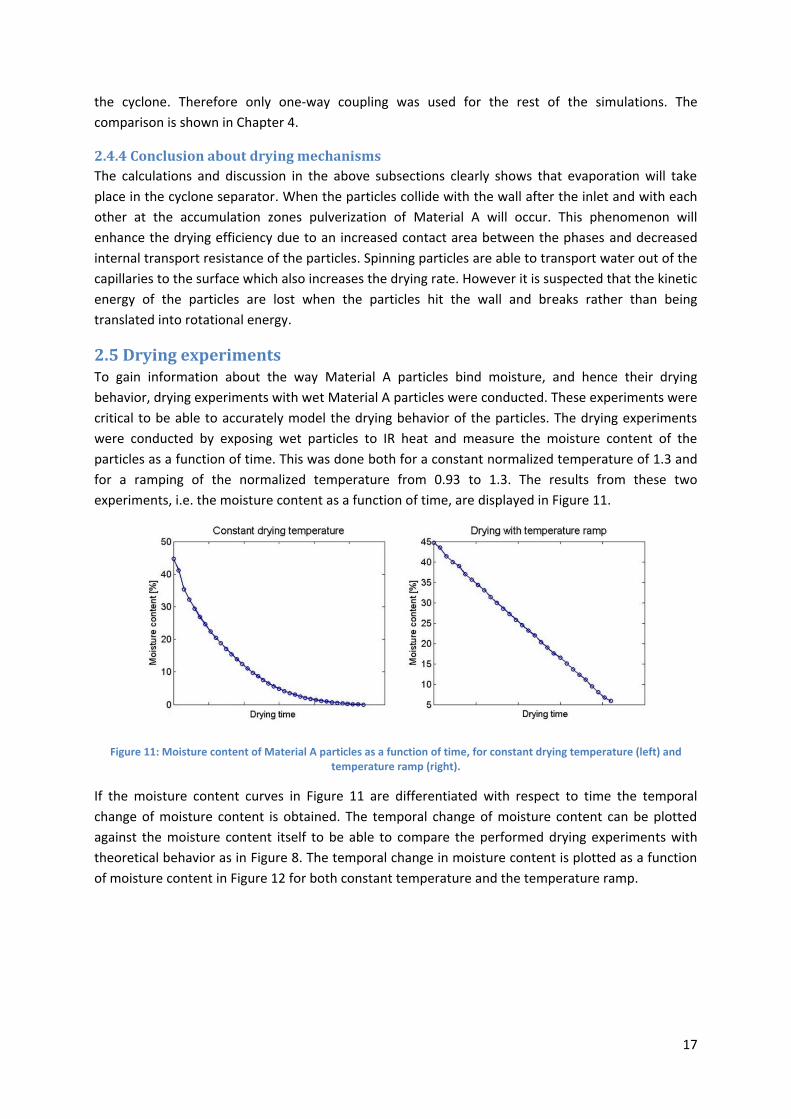
2.5 Drying experiments To gain information about the way Material A particles bind moisture, and hence their drying
behavior, drying experiments with wet Material A particles were conducted. These experiments were
critical to be able to accurately model the drying behavior of the particles. The drying experiments
were conducted by exposing wet particles to IR heat and measure the moisture content of the
particles as a function of time. This was done both for a constant normalized temperature of 1.3 and
for a ramping of the normalized temperature from 0.93 to 1.3. The results from these two
experiments, i.e. the moisture content as a function of time, are displayed in Figure 11.
Figure 11: Moisture content of Material A particles as a function of time, for constant drying temperature (left) and temperature ramp (right).
If the moisture content curves in Figure 11 are differentiated with respect to time the temporal
change of moisture content is obtained. The temporal change of moisture content can be plotted
against the moisture content itself to be able to compare the performed drying experiments with
theoretical behavior as in Figure 8. The temporal change in moisture content is plotted as a function
of moisture content in Figure 12 for both constant temperature and the temperature ramp.
18
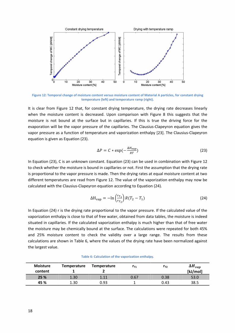
Figure 12: Temporal change of moisture content versus moisture content of Material A particles, for constant drying temperature (left) and temperature ramp (right).
It is clear from Figure 12 that, for constant drying temperature, the drying rate decreases linearly
when the moisture content is decreased. Upon comparison with Figure 8 this suggests that the
moisture is not bound at the surface but in capillaries. If this is true the driving force for the
evaporation will be the vapor pressure of the capillaries. The Clausius-Clapeyron equation gives the
vapor pressure as a function of temperature and vaporization enthalpy [23]. The Clausius-Clapeyron
equation is given as Equation (23).
(
) (23)
In Equation (23), C is an unknown constant. Equation (23) can be used in combination with Figure 12
to check whether the moisture is bound in capillaries or not. First the assumption that the drying rate
is proportional to the vapor pressure is made. Then the drying rates at equal moisture content at two
different temperatures are read from Figure 12. The value of the vaporization enthalpy may now be
calculated with the Clausius-Clapeyron equation according to Equation (24).
(
) ( ) (24)
In Equation (24) r is the drying rate proportional to the vapor pressure. If the calculated value of the
vaporization enthalpy is close to that of free water, obtained from data tables, the moisture is indeed
situated in capillaries. If the calculated vaporization enthalpy is much higher than that of free water
the moisture may be chemically bound at the surface. The calculations were repeated for both 45%
and 25% moisture content to check the validity over a large range. The results from these
calculations are shown in Table 6, where the values of the drying rate have been normalized against
the largest value.
Table 6: Calculation of the vaporization enthalpy.
Moisture content
Temperature 1
Temperature 2
rT1 rT2
[kJ/mol]
25 % 1.30 1.11 0.67 0.38 53.0 45 % 1.30 0.93 1 0.43 38.5
19
The value of the vaporization enthalpy for water is taken from data tables at normalized
temperatures of 1.2 and 1.11 respectively for 25% and 45% moisture content. The values are taken
from Marsh [24]. From these tables it was found that the value of the vaporization enthalpy was
around 43kJ/mol and since this value is close to the calculated values the conclusion that the
moisture is indeed bound in capillaries could be drawn. Therefore the temporal change of moisture
content in the particles could be expressed as a function of moisture content and the vapor pressure
defined in Equation (23). Comparing to the general expression for the drying rate defined by [7] the
final expression for the drying rate can be expressed as Equation (25).
( ) (
) (25)
In Equation (25) mv and mp are the mass of the evaporated moisture and the wet solid respectively
whereas W is the moisture content expressed on a wet mass basis. It is the rate expression defined
on the right hand side of Equation (25) that is used to model the evaporation of moisture from the
particles in the simulations performed. The first part of the right hand side of Equation (25), i.e.
( ), is a linear fitting to the data for a constant normalized drying
temperature of 1.3 in Figure 12. The second part of the right hand side of Equation (25), i.e.
(
), is used to describe the temperature dependence. Hence the unknown
constant C in Equation (23) takes the value of 2.5e6.
2.6 Solution procedure The first step in the modeling procedure of the cyclone separator is to solve the gas flow field. Before
solving, the instantaneous governing equations for mass, momentum and energy, defined in
Appendix C.1, are averaged. The averaging is performed since the instantaneous equations are too
computationally expensive to solve directly. Averaging of the governing equations means that the
instantaneous variables are divided into a mean and a fluctuating part, before they are inserted into
the governing equations. Upon averaging the problem of closure arises due to the formation of the
Reynolds stress terms. The closure problem means that the number of variables is greater than the
number of equations. Different turbulence models deal with the closure problem in different ways.
The RSM model solves transport equations for the Reynolds stresses whereas two-equation models
use the Boussinesq approximation for the Reynolds stresses and hence only solves transport
equations for the turbulent kinetic energy and the energy-dissipation rate. The additional transport
equations result in that the RSM model is more accurate but also more computationally expensive
than two-equation models [21]. According to Hoekstra [25] the RSM model should be used for
cyclone separators since it captures the vertical velocities better than two-equation models when
compared to experiments.
However, due to computational power limitations, a two-equation model had to be used. The RNG k-
model was chosen since it is recommended for swirling flows. The RNG k- model includes a
source term in the transport equation for the energy-dissipation rate that is not included in other
two-equation models. This source term results in less destruction of energy-dissipation rate which in
turn will increase the turbulent kinetic energy and decrease the turbulent viscosity. Decreased
turbulent viscosity implies that the RNG k- model is less dissipative than other two-equation
models and should therefore be used for swirling flows [21]. To model the turbulence in the
boundary layers in the near-wall region, so called enhanced wall-treatment was employed. The
20
enhanced wall-treatment treats the flow in different ways depending on the value of the
dimensionless wall-distance y+. Hence little consideration about not having a too low value of y+ for
the first cell layer has to be taken during mesh construction [3].
The numerical method chosen for the simulations was the pressure-based solver. This means that a
pressure equation is obtained by manipulation of the momentum conservation equation using the
continuity equation. The flow is then solved using a coupled algorithm. The first step in the coupled
algorithm is to solve a coupled system of the momentum equations and the pressure equation.
Thereafter the mass flux is updated and the scalar transport equations are solved. A convergence
check is performed and if the solution is not converged the fluid properties are updated and the
algorithm is run again. This procedure is repeated until convergence has been reached. The coupled
algorithm was used since it improves the rate of convergence compared to if the momentum and
pressure equations had been solved separately [3], [21].
The values of scalars are stored in the cell center, but values at the cell faces are also needed during
the iterations. During the simulations of this thesis the second order upwind differencing scheme was
employed to interpolate the cell face values of scalars. When calculating the value at a cell face the
second order upwind scheme takes into account the cell values from two adjacent cells in the
upwind direction. Upwind differencing schemes are preferable due to the high gas velocities inside
the cyclone meaning that the cell values should be more influenced by the upstream than the
downstream conditions due to the strong convection. The second order scheme was chosen over the
first order scheme in order to avoid numerical diffusion. Second order schemes were used to
interpolate values of density, momentum, swirl velocity, turbulent kinetic energy, turbulent
dissipation-rate and energy to the cell faces. To interpolate the cell face values of pressure the
PRESTO! scheme was used, since it is recommended for swirling flows. The PRESTO! scheme
calculates the pressure on the cell faces by using a mesh that is shifted to have the new cell centers
at the old cell faces [3], [21].
To advance the solution between iterations so called pseudo transient under-relaxation was used.
The pseudo transient under-relaxation can be used for steady-state simulations and is a form of
implicit under-relaxation. The under-relaxation determines how much the new value of the cell is
influenced by the value obtained from the solver in comparison with that from the previous iteration.
If the new cell value is influenced too much by the solver value the risk for divergence is high. On the
other hand, if the new cell value is too influenced by the value from the previous iteration,
convergence will be slow. The pseudo transient under-relaxation is controlled using an automatically
determined pseudo time-step. The automatic pseudo time-step is defined as the minimum of the
convective, dynamic, gravitational, rotational, compressible and viscous timescale. For definitions of
these timescales see [3]. When using pseudo transient under-relaxation the number of iterations
needed to reach convergence is lower than for explicit under-relaxation [3], [21].
A more detailed description of the governing equations, averaging procedure, turbulence model and
wall-treatment are given in Appendix C.
2.7 Discrete phase modeling In this thesis so called Lagrangian particle tracking was used. The use of Lagrangian tracking implies
that each particle is tracked individually by solving the equation of motion for that particle. This
modeling approach is also known as discrete phase modeling or DPM. The modeling approach when
21
DPM is used differs depending on whether one-way or two-way momentum coupling between the
particles and the continuous phase exists. The first step is however independent of the type of
coupling. First the flow field is solved without introducing any particles into the domain. Then the
particles are released into the flow field. For one-way coupling this can be done in the Fluent
postprocessor since the particles will not affect the flow field. This means that only the equation of
motion for each particle is solved. For two-way coupling the flow field is updated after the particles
have been introduced. The coupling takes the form of a source term in the momentum conservation
equations of the fluid. When the flow field has been updated the particles are allowed to advance in
the domain and the flow field is updated again [3], [21]. The particle tracking is described in more
detail in Subsection 2.7.1.
2.7.1 Forces acting on the particles
In this section the equation of motion for a single particle adopted in the Lagrangian framework will
be stated in Subsection 2.7.1.1. In Subsections 2.7.1.2-2.7.1.10 a short description of the different
forces acting on the particles will be given, and an evaluation of their importance is made.
2.7.1.1 Equation of motion
In the Lagrangian framework the particles are tracked on an individual level. The time rate of change
of momentum is equal to the sum of forces acting on the particle in agreement with Newton’s
second law. The equation of motion for a single particle can be written as Equation (26) [21].
∑ (26)
In Equation (26) d denotes the dispersed phase and i denotes particle i. The forces taken into
consideration are the drag, pressure and shear, virtual mass, Basset, buoyancy, lift, thermophoretic,
turbulent dispersion and Brownian forces. Simulations including all of the above forces will be very
time consuming and it is therefore important to assess which forces that affects the particle enough
to be included in the simulations. These forces are described in more detail in the following
subsections, and an assessment of their importance is made.
2.7.1.2 Drag force
The drag force arises when a relative velocity between the dispersed and the continuous phase
exists. The drag force can be written according to Equation (27) [3].
| |( ) (27)
As mentioned in Section 2.1 the drag force is what counteracts the centrifugal force acting on the
particles inside the cyclone. Hence the drag force was included in the simulations.
In the Ansys Fluent software used for the simulations the drag coefficient is calculated according to
Equation (28) [3].
(28)
In Equation (28) Rep is the particle Reynolds number. Values for the coefficients a1, a2 and a3 were
described by Morsi and Alexander with different values for different particle Reynolds number [3],
[26]. The particle Reynolds number is defined as Equation (29) [3].
22
( )
(29)
2.7.1.3 Pressure and shear force
The pressure and shear force arises when pressure and shear gradients exist over the particle
surface. This force can be expressed as Equation (30) [21].
(
) (30)
Since the volume of the particles is very small and the pressure variations inside the cyclone
separator are small the gradients over the particle surfaces should not be very large and the pressure
and shear forces were therefore considered negligible.
2.7.1.4 Virtual mass force
The added mass force is a force that arises when a fraction of the fluid surrounding the particle is
accelerated together with the particle. When fluid accelerates together with the particle the particle
appears to be heavier than it actually is which adds inertia to the system. The added mass force is
important for large particles since they will accelerate a larger fraction of the fluid. Fluids of high
density will also increase the added mass force since higher density means larger mass of a specific
volume of the fluid [16]. The virtual mass force can be expressed as Equation (31) [21].
( ) (31)
In Equation (31) CVM is the virtual mass coefficient that describes the ratio of the continuous phase
volume that is accelerated together with the particle to the particle volume. This coefficient is usually
in the order of 0.5 [21]. Since the density of the continuous phase is much smaller than the discrete
phase density and the particles were very small the added mass force was neglected in the
simulations.
2.7.1.5 Basset force
The Basset force arises when there is a change in relative velocity between the dispersed and the
continuous phase due to a delay in the boundary layer development. Boundary layer growth will
decelerate the flow by viscous friction and hence the Basset force is important for very viscous fluids
and particles of large projected area. The Basset force can be expressed as Equation (32) [16].
√ ∫
√
( – ) (32)
Since both the density and viscosity of air is small and the particles have a small diameter the Basset
force was assumed negligible and was excluded from the simulations.
2.7.1.6 Buoyancy and gravity force
The buoyancy force arises when a body is emerged in a fluid and hence displaces the fluid. The
displaced fluid acts to lift the body. The buoyancy force can be written as Equation (33) [21].
(33)
Since both the particle volume and the fluid density are small the buoyancy force was considered
negligible. However the gravity was included as the gravitational force acting on the particles.
23
2.7.1.7 Lift forces
There are two kinds of lift forces acting on the particles, namely the Magnus and the Saffman lift
forces. The Magnus lift force arises due to rotation of the particles. When a particle rotates the
relative velocity between the particle and the fluid becomes smaller on one side of the particle and
hence a lift force in the direction of the smallest relative velocity occurs. If the rotational vector is
normal to the relative velocity vector the Magnus lift force can be written as Equation (34) [16].
( ) (34)
As discussed in Section 2.4.2 high rotational velocities of the particles may occur in the cyclone.
However the particle volume is very small meaning that the Magnus lift force can be neglected in the
simulations.
The Saffman lift force arises when the particles encounter a velocity gradient. A velocity gradient
implies that the flow on different sides of the particles have different velocities. This means that the
side of the particle that experiences the highest flow velocity will experience a lower pressure than
the other side of the particle and hence a lift force in the direction of the lowest pressure arises. The
Saffman lift force can be expressed as Equation (35) [16].
| – |√
(35)
The particle diameter and the fluid viscosity are small. Also, because of the small particle diameter
the velocity gradient over the particle should not be of significant magnitude and therefore the
Saffman lift force was neglected in the simulations.
2.7.1.8 Thermophoretic force
When a temperature gradient exists over the particle the thermophoretic force arises. Fluid
molecules will collide with the particle. If these collisions last long enough for the fluid molecules to
reach the temperature of the particle surface before they leave, the thermophoretic force will arise.
Fluid molecules with a temperature higher than the surface temperature will be cooled and hence
leave the particle with a lower velocity than the impact velocity. On the other hand, fluid molecules
with a temperature lower than the particle surface temperature will leave the particle with a velocity
higher than the impact velocity. Hence a net force in the opposite direction of the temperature
gradient is experienced by the particle. For spherical particles and in an ideal gas flow the
thermophoretic force can be expressed as Equation (36) [3], [21].
(
)
( )(
)
(36)
In Equation (36) kp is the thermal conductivity of the particle and ct, cs and cm are constants. The fluid
thermal conductivity, labeled k in Equation (36), should be based on translational energy only and
can hence be calculated according to Equation (37) [3].
(37)
Kn in Equation 37 denotes the Knudsen number which is defined as Equation (38) [3].
24
(38)
In Equation (38) denotes the mean free path of the gas, i.e. the average distance travelled by a
molecule between collisions [3]. These molecule-particle collisions will only be able to affect very
small particles [21]. The particles simulated in this thesis are indeed small, but nonetheless they are
not sub-micron particles. Therefore the assessment that the thermophoretic force would not affect
the particles to any significant extent was made and the force was excluded from the simulations.
2.7.1.9 Turbulent dispersion
Particles in a turbulent flow will be dispersed due to fluctuating fluid velocities. When modeling
turbulent dispersion a fluctuating component is added to the particle velocity. The fluctuating part is
modeled as a random number with normal distribution multiplied by the turbulent velocity according
to Equation (39) [16].
√
(39)
In Equation (39) is the aforementioned normally distributed random number. Since the turbulent
kinetic energy is a scalar all three components of the fluctuating part will be equal and hence
isotropic dispersion is predicted. This is a random walk model. The particle is transported by an eddy
until it dissipates or until the particle has passed through the eddy and then travels with another
eddy. The lifetime of eddies is calculated using the Lagrangian integral time scale defined in Equation
(40) [3].
(40)
In Equation (40) CL is a constant that takes an approximate value of 0.15 for the k- models. The
eddy lifetime was set as random in the simulations and was hence calculated according to Equation
(41) [3].
( ) (41)
In Equation (41) r is a uniform random number taking values between 0 and 1 [3]. Since the
fluctuating part of the velocity is modeled as a random process a statistical average over a number of
simulations is necessary to obtain a reliable result for the particle tracks [16]. Turbulent dispersion
was incorporated into the simulations and five different tries were run to obtain a statistical average.
However, no difference in the number of particles exiting the cyclone was observed between the
different simulations.
2.7.1.10 Brownian motion
Brownian motion arises because of individual collisions between molecules and particles. These
collisions will lead to a sort of particle diffusion. Brownian motion is only important for sub-micron
particles [21]. The modeling of Brownian motion resembles that of turbulent dispersion. Brownian
motion is modeled as white noise. The force components are modeled with the product of a
Gaussian distributed random number and the square root of the spectral intensity. Since only a small
fraction of the particles have a diameter in the order of 1 micron the Brownian motion was
considered superfluous for the simulations. Also Brownian motion should be included only for
25
laminar flows. Turbulent dispersion replaces the Brownian motion in turbulent flows such as that in
the cyclone [3].
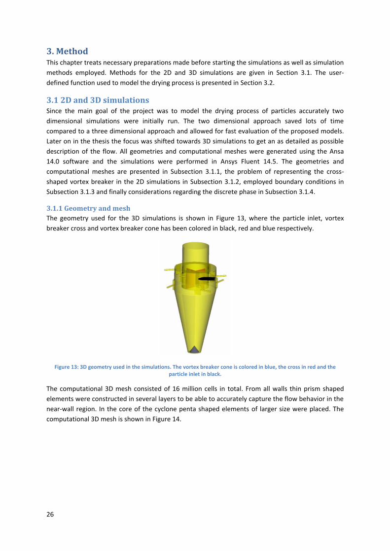
26
3. Method This chapter treats necessary preparations made before starting the simulations as well as simulation
methods employed. Methods for the 2D and 3D simulations are given in Section 3.1. The user-
defined function used to model the drying process is presented in Section 3.2.
3.1 2D and 3D simulations Since the main goal of the project was to model the drying process of particles accurately two
dimensional simulations were initially run. The two dimensional approach saved lots of time
compared to a three dimensional approach and allowed for fast evaluation of the proposed models.
Later on in the thesis the focus was shifted towards 3D simulations to get an as detailed as possible
description of the flow. All geometries and computational meshes were generated using the Ansa
14.0 software and the simulations were performed in Ansys Fluent 14.5. The geometries and
computational meshes are presented in Subsection 3.1.1, the problem of representing the cross-
shaped vortex breaker in the 2D simulations in Subsection 3.1.2, employed boundary conditions in
Subsection 3.1.3 and finally considerations regarding the discrete phase in Subsection 3.1.4.
3.1.1 Geometry and mesh
The geometry used for the 3D simulations is shown in Figure 13, where the particle inlet, vortex
breaker cross and vortex breaker cone has been colored in black, red and blue respectively.
Figure 13: 3D geometry used in the simulations. The vortex breaker cone is colored in blue, the cross in red and the particle inlet in black.
The computational 3D mesh consisted of 16 million cells in total. From all walls thin prism shaped
elements were constructed in several layers to be able to accurately capture the flow behavior in the
near-wall region. In the core of the cyclone penta shaped elements of larger size were placed. The
computational 3D mesh is shown in Figure 14.
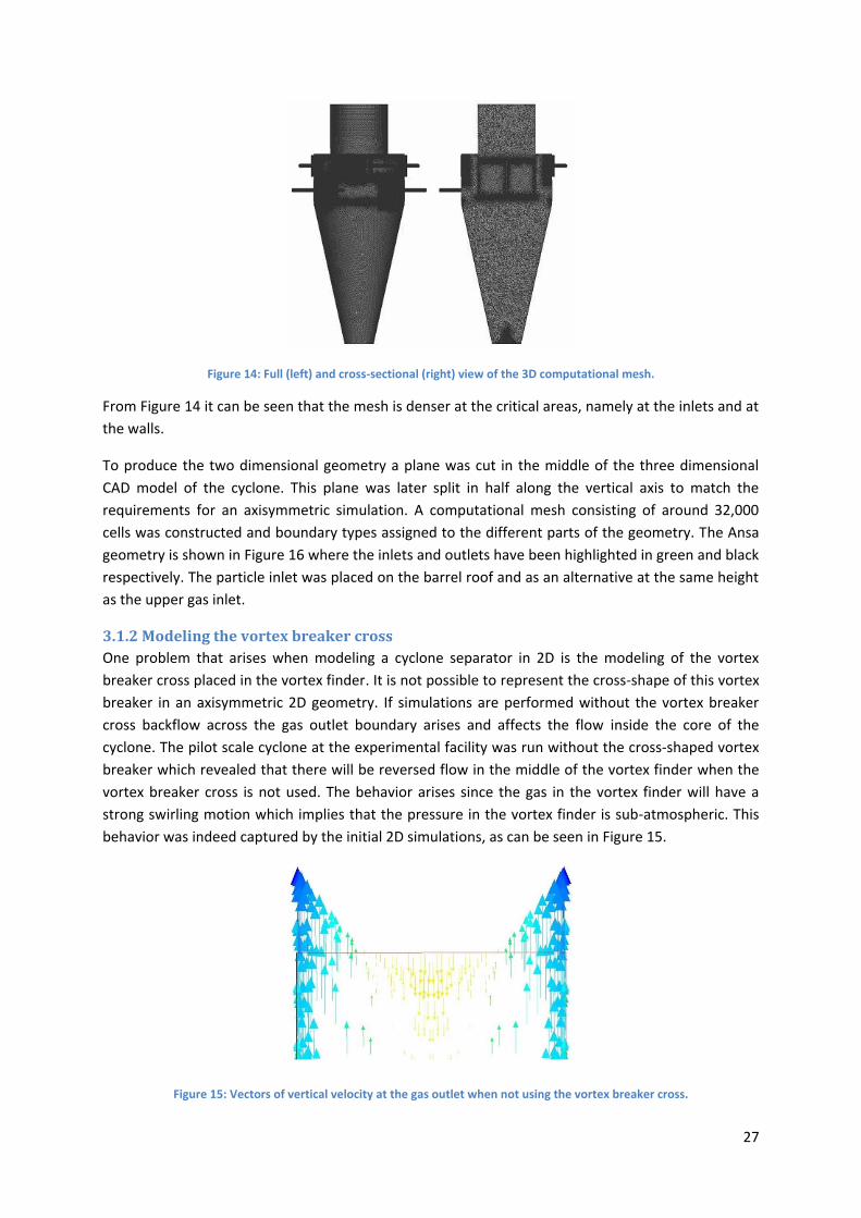
27
Figure 14: Full (left) and cross-sectional (right) view of the 3D computational mesh.
From Figure 14 it can be seen that the mesh is denser at the critical areas, namely at the inlets and at
the walls.
To produce the two dimensional geometry a plane was cut in the middle of the three dimensional
CAD model of the cyclone. This plane was later split in half along the vertical axis to match the
requirements for an axisymmetric simulation. A computational mesh consisting of around 32,000
cells was constructed and boundary types assigned to the different parts of the geometry. The Ansa
geometry is shown in Figure 16 where the inlets and outlets have been highlighted in green and black
respectively. The particle inlet was placed on the barrel roof and as an alternative at the same height
as the upper gas inlet.
3.1.2 Modeling the vortex breaker cross
One problem that arises when modeling a cyclone separator in 2D is the modeling of the vortex
breaker cross placed in the vortex finder. It is not possible to represent the cross-shape of this vortex
breaker in an axisymmetric 2D geometry. If simulations are performed without the vortex breaker
cross backflow across the gas outlet boundary arises and affects the flow inside the core of the
cyclone. The pilot scale cyclone at the experimental facility was run without the cross-shaped vortex
breaker which revealed that there will be reversed flow in the middle of the vortex finder when the
vortex breaker cross is not used. The behavior arises since the gas in the vortex finder will have a
strong swirling motion which implies that the pressure in the vortex finder is sub-atmospheric. This
behavior was indeed captured by the initial 2D simulations, as can be seen in Figure 15.
Figure 15: Vectors of vertical velocity at the gas outlet when not using the vortex breaker cross.

28
However the focus was on representing the complete 3D cyclone as a 2D model to save
computational time but still obtain representative results. To model the vortex breaker cross a cell
zone inside the vortex finder was created. A fixed value of zero swirl velocity was set for this cell zone
and hence the vortex was successfully broken. The cell zone used to model the vortex breaker cross
is shown in Figure 16, colored in red.
Figure 16: 2D geometry used in the simulations. The cell zone used for modeling the vortex breaker cross is colored in red, gas inlets are colored in green and outlets in black.
Using the modeled vortex breaker cross resulted in that the vortex was broken and hence the
pressure difference across the outlet was significantly reduced. As a consequence of the reduced
pressure difference no backflow into the vortex finder was observed. The zero-velocity cell zone was
therefore used throughout the different 2D simulations.
3.1.3 Boundary conditions
The boundary conditions for the gas and dust outlet were chosen as pressure outlet and pressure
inlet respectively, both with a gauge pressure equal to the atmospheric. The choice of representing
the dust outlet as a pressure inlet was made because air is leaking in to the cyclone due to the sub-
atmospheric pressure that exists in the bottom end of the cyclone.
For the gas inlets the velocity inlet boundary condition was employed for the 2D axisymmetric swirl
case. The inlet will be represented as a 360° ring around the entire cyclone due to the axisymmetry.
This implies that some decisions about the inlet velocity components have to be taken. The vertical
velocity component was set to zero whereas the radial velocity component was modified to give the
experimentally observed volume flow rate into the cyclone. It was found that a normalized radial
velocity of 0.004 resulted in the desired volume flow rate. The swirl, i.e. tangential, normalized
component of the velocity was calculated to 1 by dividing the experimentally observed volume flow
rate by the nozzle area. The inlet temperature was chosen as the experimentally measured one.
The boundary conditions used for the 3D simulations were almost identical as in the 2D case. The
only difference was for the gas and particle inlets. Instead of velocity inlets the gas inlets were
treated as pressure inlets. Hence a pressure was defined at the inlets instead of velocity components
as in the 2D case. The reason for this was the inlet pressure could be measured at the test facility.
Gas is used to transport the particles into the cyclone from the particle inlet. Therefore the gas
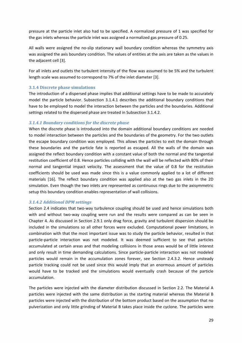
29
pressure at the particle inlet also had to be specified. A normalized pressure of 1 was specified for
the gas inlets whereas the particle inlet was assigned a normalized gas pressure of 0.25.
All walls were assigned the no-slip stationary wall boundary condition whereas the symmetry axis
was assigned the axis boundary condition. The values of entities at the axis are taken as the values in
the adjacent cell [3].
For all inlets and outlets the turbulent intensity of the flow was assumed to be 5% and the turbulent
length scale was assumed to correspond to 7% of the inlet diameter [3].
3.1.4 Discrete phase simulations
The introduction of a dispersed phase implies that additional settings have to be made to accurately
model the particle behavior. Subsection 3.1.4.1 describes the additional boundary conditions that
have to be employed to model the interaction between the particles and the boundaries. Additional
settings related to the dispersed phase are treated in Subsection 3.1.4.2.
3.1.4.1 Boundary conditions for the discrete phase
When the discrete phase is introduced into the domain additional boundary conditions are needed
to model interaction between the particles and the boundaries of the geometry. For the two outlets
the escape boundary condition was employed. This allows the particles to exit the domain through
these boundaries and the particle fate is reported as escaped. All the walls of the domain was
assigned the reflect boundary condition with a constant value of both the normal and the tangential
restitution coefficient of 0.8. Hence particles colliding with the wall will be reflected with 80% of their
normal and tangential impact velocity. The assessment that the value of 0.8 for the restitution
coefficients should be used was made since this is a value commonly applied to a lot of different
materials [16]. The reflect boundary condition was applied also at the two gas inlets in the 2D
simulation. Even though the two inlets are represented as continuous rings due to the axisymmetric
setup this boundary condition enables representation of wall collisions.
3.1.4.2 Additional DPM settings
Section 2.4 indicates that two-way turbulence coupling should be used and hence simulations both
with and without two-way coupling were run and the results were compared as can be seen in
Chapter 4. As discussed in Section 2.9.1 only drag force, gravity and turbulent dispersion should be
included in the simulations so all other forces were excluded. Computational power limitations, in
combination with that the most important issue was to study the particle behavior, resulted in that
particle-particle interaction was not modeled. It was deemed sufficient to see that particles
accumulated at certain areas and that modeling collisions in those areas would be of little interest
and only result in time demanding calculations. Since particle-particle interaction was not modeled
particles would remain in the accumulation zones forever, see Section 2.4.3.2. Hence unsteady
particle tracking could not be used since this would imply that an enormous amount of particles
would have to be tracked and the simulations would eventually crash because of the particle
accumulation.
The particles were injected with the diameter distribution discussed in Section 2.2. The Material A
particles were injected with the same distribution as the starting material whereas the Material B
particles were injected with the distribution of the bottom product based on the assumption that no
pulverization and only little grinding of Material B takes place inside the cyclone. The particles were
30
released from the particle inlet with a normalized velocity of 0.0058 normal to the surface. The
amount of particles injected corresponded to what had been fed to the cyclone during experiments.
To model the evaporation of water from the solid particles so called multicomponent particles were
used in combination with a user defined function. Multicomponent particles allow for injection of
particles consisting of more than one substance. However in Fluent only liquid particles can be
represented as multicomponent particles. It is therefore necessary to first create a multicomponent
particle consisting of water and an additional liquid to later change the properties of the additional
liquid to represent that of the actual solid, for example by setting a very high evaporation
temperature. The UDF described in Section UDF was hooked to the solver to model the evaporation
process of the water. The procedure of creating a multicomponent injection and hooking the UDF to
the solver is described in more detail in Appendix B.
3.3 User-defined function Since the built in multicomponent evaporation model in Fluent treats the particles as droplets the
evaporation rate of water will not be equal to that observed for evaporation from solid particles.
Therefore a user-defined function calculating the evaporation rate had to be written. Ansys provides
a template for multicomponent evaporation which was used as a starting point. The main changes to
this UDF template made were replacing the expression for the evaporation rate by the expression
defined as Equation (25) and removing the part of the template corresponding to boiling since boiling
will not occur inside the cyclone.
One drawback of the employed UDF is that it was not able to keep the diameter of the particles
constant as the evaporation progressed. Also the density of the particles increased instead of
decreased when water was evaporated. These two drawbacks were due to the way the
multicomponent particle model calculate the particle diameter and density. The problem arises since
the multicomponent particle model is developed for liquid droplets for which the diameter will
decrease during the evaporation process. When it comes to the density it is calculated using a
volume weighted mixing law meaning that the density of the particles will increase when the light
component water is evaporated [3]. The UDF is appended as Appendix A.
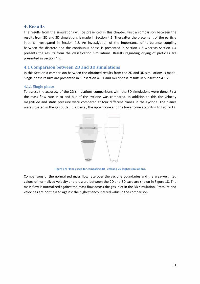
31
4. Results The results from the simulations will be presented in this chapter. First a comparison between the
results from 2D and 3D simulations is made in Section 4.1. Thereafter the placement of the particle
inlet is investigated in Section 4.2. An investigation of the importance of turbulence coupling
between the discrete and the continuous phase is presented in Section 4.3 whereas Section 4.4
presents the results from the classification simulations. Results regarding drying of particles are
presented in Section 4.5.
4.1 Comparison between 2D and 3D simulations In this Section a comparison between the obtained results from the 2D and 3D simulations is made.
Single phase results are presented in Subsection 4.1.1 and multiphase results in Subsection 4.1.2.
4.1.1 Single phase
To assess the accuracy of the 2D simulations comparisons with the 3D simulations were done. First
the mass flow rate in to and out of the cyclone was compared. In addition to this the velocity
magnitude and static pressure were compared at four different planes in the cyclone. The planes
were situated in the gas outlet, the barrel, the upper cone and the lower cone according to Figure 17.
Figure 17: Planes used for comparing 3D (left) and 2D (right) simulations.
Comparisons of the normalized mass flow rate over the cyclone boundaries and the area-weighted
values of normalized velocity and pressure between the 2D and 3D case are shown in Figure 18. The
mass flow is normalized against the mass flow across the gas inlet in the 3D simulation. Pressure and
velocities are normalized against the highest encountered value in the comparison.
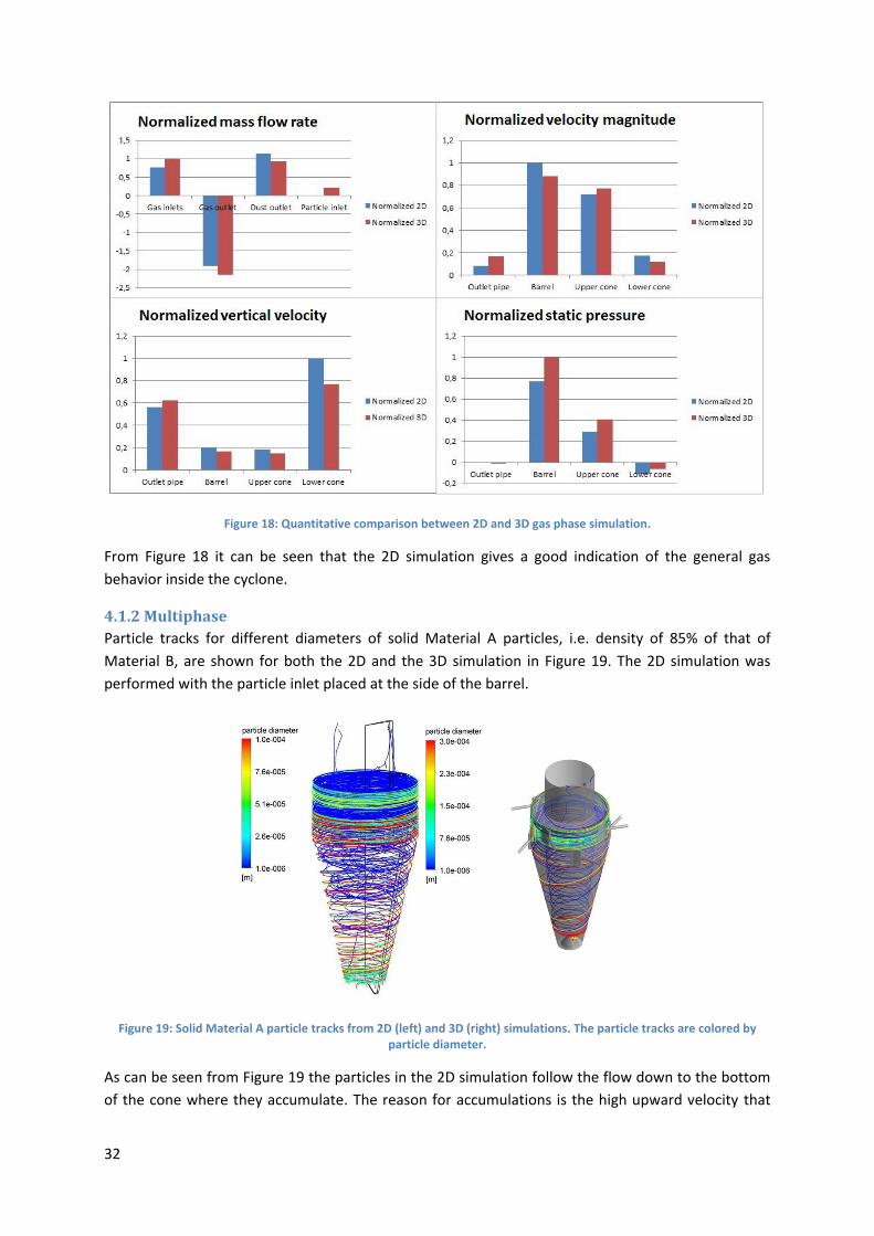
32
Figure 18: Quantitative comparison between 2D and 3D gas phase simulation.
From Figure 18 it can be seen that the 2D simulation gives a good indication of the general gas
behavior inside the cyclone.
4.1.2 Multiphase
Particle tracks for different diameters of solid Material A particles, i.e. density of 85% of that of
Material B, are shown for both the 2D and the 3D simulation in Figure 19. The 2D simulation was
performed with the particle inlet placed at the side of the barrel.
Figure 19: Solid Material A particle tracks from 2D (left) and 3D (right) simulations. The particle tracks are colored by particle diameter.
As can be seen from Figure 19 the particles in the 2D simulation follow the flow down to the bottom
of the cone where they accumulate. The reason for accumulations is the high upward velocity that
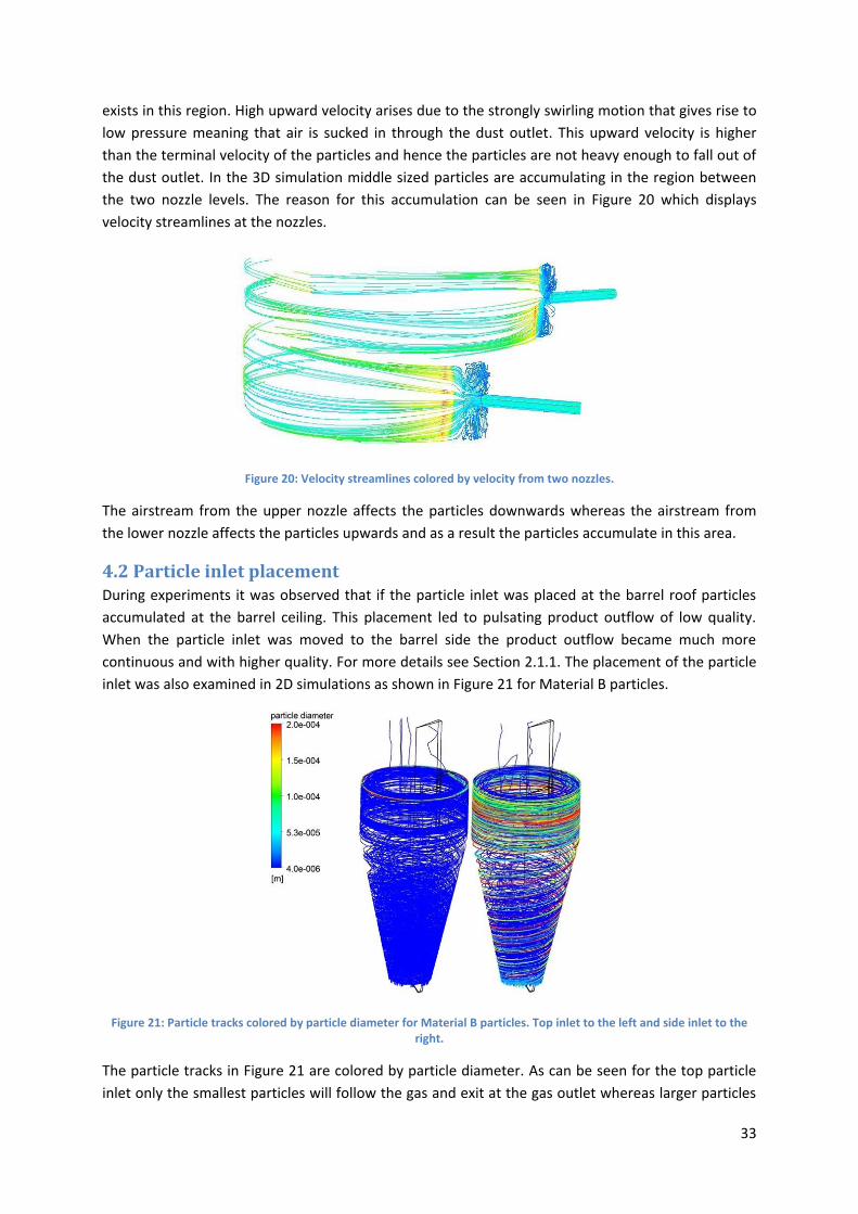
33
exists in this region. High upward velocity arises due to the strongly swirling motion that gives rise to
low pressure meaning that air is sucked in through the dust outlet. This upward velocity is higher
than the terminal velocity of the particles and hence the particles are not heavy enough to fall out of
the dust outlet. In the 3D simulation middle sized particles are accumulating in the region between
the two nozzle levels. The reason for this accumulation can be seen in Figure 20 which displays
velocity streamlines at the nozzles.
Figure 20: Velocity streamlines colored by velocity from two nozzles.
The airstream from the upper nozzle affects the particles downwards whereas the airstream from
the lower nozzle affects the particles upwards and as a result the particles accumulate in this area.
4.2 Particle inlet placement During experiments it was observed that if the particle inlet was placed at the barrel roof particles
accumulated at the barrel ceiling. This placement led to pulsating product outflow of low quality.
When the particle inlet was moved to the barrel side the product outflow became much more
continuous and with higher quality. For more details see Section 2.1.1. The placement of the particle
inlet was also examined in 2D simulations as shown in Figure 21 for Material B particles.
Figure 21: Particle tracks colored by particle diameter for Material B particles. Top inlet to the left and side inlet to the right.
The particle tracks in Figure 21 are colored by particle diameter. As can be seen for the top particle
inlet only the smallest particles will follow the gas and exit at the gas outlet whereas larger particles
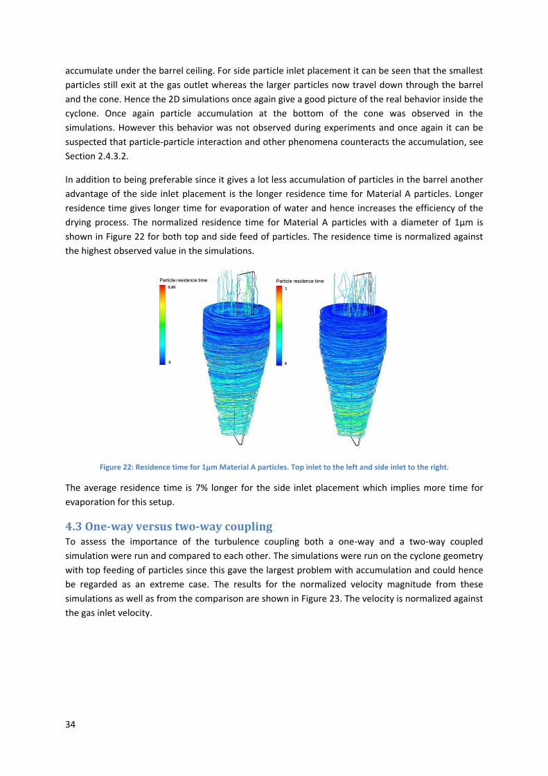
34
accumulate under the barrel ceiling. For side particle inlet placement it can be seen that the smallest
particles still exit at the gas outlet whereas the larger particles now travel down through the barrel
and the cone. Hence the 2D simulations once again give a good picture of the real behavior inside the
cyclone. Once again particle accumulation at the bottom of the cone was observed in the
simulations. However this behavior was not observed during experiments and once again it can be
suspected that particle-particle interaction and other phenomena counteracts the accumulation, see
Section 2.4.3.2.
In addition to being preferable since it gives a lot less accumulation of particles in the barrel another
advantage of the side inlet placement is the longer residence time for Material A particles. Longer
residence time gives longer time for evaporation of water and hence increases the efficiency of the
drying process. The normalized residence time for Material A particles with a diameter of 1µm is
shown in Figure 22 for both top and side feed of particles. The residence time is normalized against
the highest observed value in the simulations.
Figure 22: Residence time for 1µm Material A particles. Top inlet to the left and side inlet to the right.
The average residence time is 7% longer for the side inlet placement which implies more time for
evaporation for this setup.
4.3 One-way versus two-way coupling To assess the importance of the turbulence coupling both a one-way and a two-way coupled
simulation were run and compared to each other. The simulations were run on the cyclone geometry
with top feeding of particles since this gave the largest problem with accumulation and could hence
be regarded as an extreme case. The results for the normalized velocity magnitude from these
simulations as well as from the comparison are shown in Figure 23. The velocity is normalized against
the gas inlet velocity.
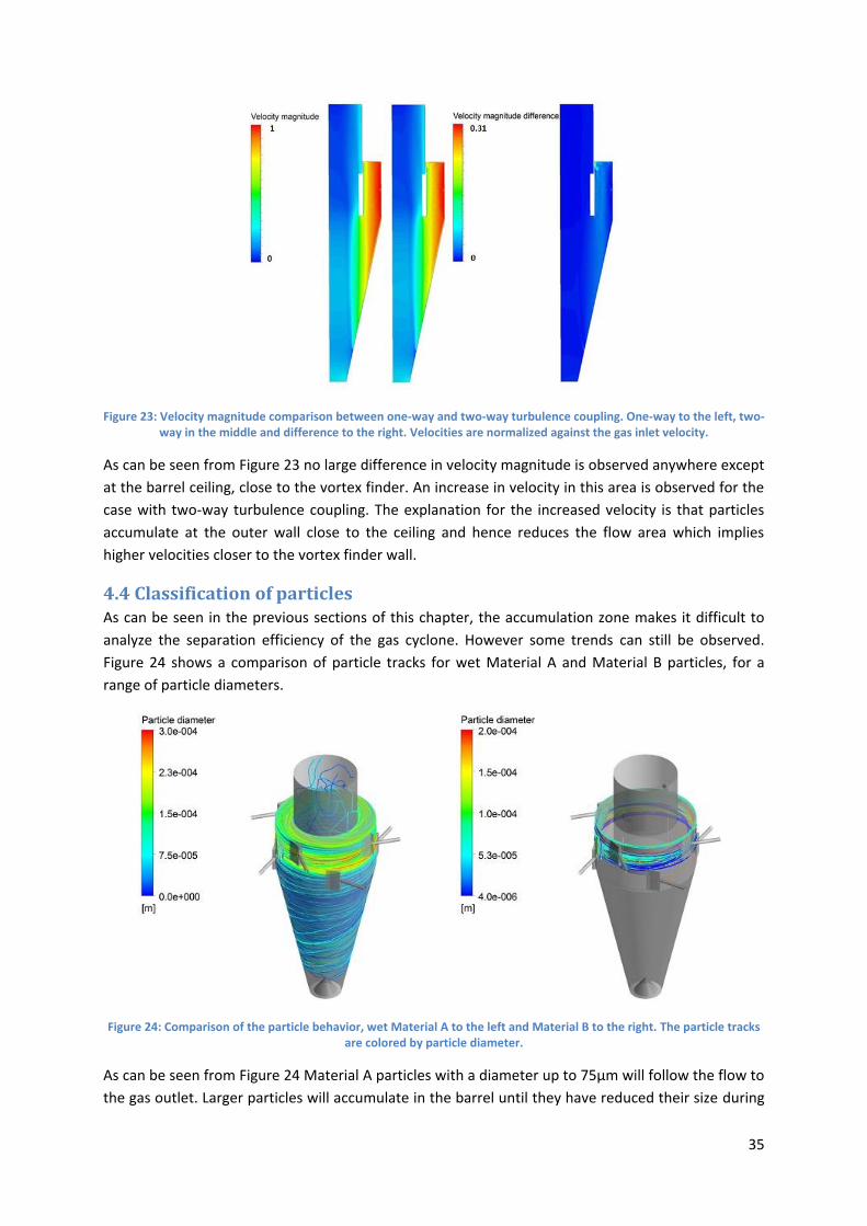
35
Figure 23: Velocity magnitude comparison between one-way and two-way turbulence coupling. One-way to the left, two-way in the middle and difference to the right. Velocities are normalized against the gas inlet velocity.
As can be seen from Figure 23 no large difference in velocity magnitude is observed anywhere except
at the barrel ceiling, close to the vortex finder. An increase in velocity in this area is observed for the
case with two-way turbulence coupling. The explanation for the increased velocity is that particles
accumulate at the outer wall close to the ceiling and hence reduces the flow area which implies
higher velocities closer to the vortex finder wall.
4.4 Classification of particles As can be seen in the previous sections of this chapter, the accumulation zone makes it difficult to
analyze the separation efficiency of the gas cyclone. However some trends can still be observed.
Figure 24 shows a comparison of particle tracks for wet Material A and Material B particles, for a
range of particle diameters.
Figure 24: Comparison of the particle behavior, wet Material A to the left and Material B to the right. The particle tracks are colored by particle diameter.
As can be seen from Figure 24 Material A particles with a diameter up to 75µm will follow the flow to
the gas outlet. Larger particles will accumulate in the barrel until they have reduced their size during
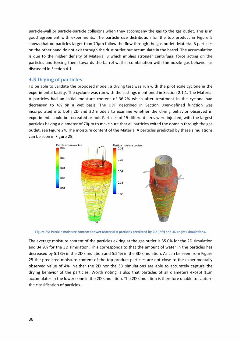
36
particle-wall or particle-particle collisions when they accompany the gas to the gas outlet. This is in
good agreement with experiments. The particle size distribution for the top product in Figure 5
shows that no particles larger than 70µm follow the flow through the gas outlet. Material B particles
on the other hand do not exit through the dust outlet but accumulate in the barrel. The accumulation
is due to the higher density of Material B which implies stronger centrifugal force acting on the
particles and forcing them towards the barrel wall in combination with the nozzle gas behavior as
discussed in Section 4.1.
4.5 Drying of particles To be able to validate the proposed model, a drying test was run with the pilot scale cyclone in the
experimental facility. The cyclone was run with the settings mentioned in Section 2.1.1. The Material
A particles had an initial moisture content of 36.2% which after treatment in the cyclone had
decreased to 4% on a wet basis. The UDF described in Section User-defined function was
incorporated into both 2D and 3D models to examine whether the drying behavior observed in
experiments could be recreated or not. Particles of 15 different sizes were injected, with the largest
particles having a diameter of 70µm to make sure that all particles exited the domain through the gas
outlet, see Figure 24. The moisture content of the Material A particles predicted by these simulations
can be seen in Figure 25.
Figure 25: Particle moisture content for wet Material A particles predicted by 2D (left) and 3D (right) simulations.
The average moisture content of the particles exiting at the gas outlet is 35.0% for the 2D simulation
and 34.9% for the 3D simulation. This corresponds to that the amount of water in the particles has
decreased by 5.13% in the 2D simulation and 5.54% in the 3D simulation. As can be seen from Figure
25 the predicted moisture content of the top product particles are not close to the experimentally
observed value of 4%. Neither the 2D nor the 3D simulations are able to accurately capture the
drying behavior of the particles. Worth noting is also that particles of all diameters except 1µm
accumulates in the lower cone in the 2D simulation. The 2D simulation is therefore unable to capture
the classification of particles.
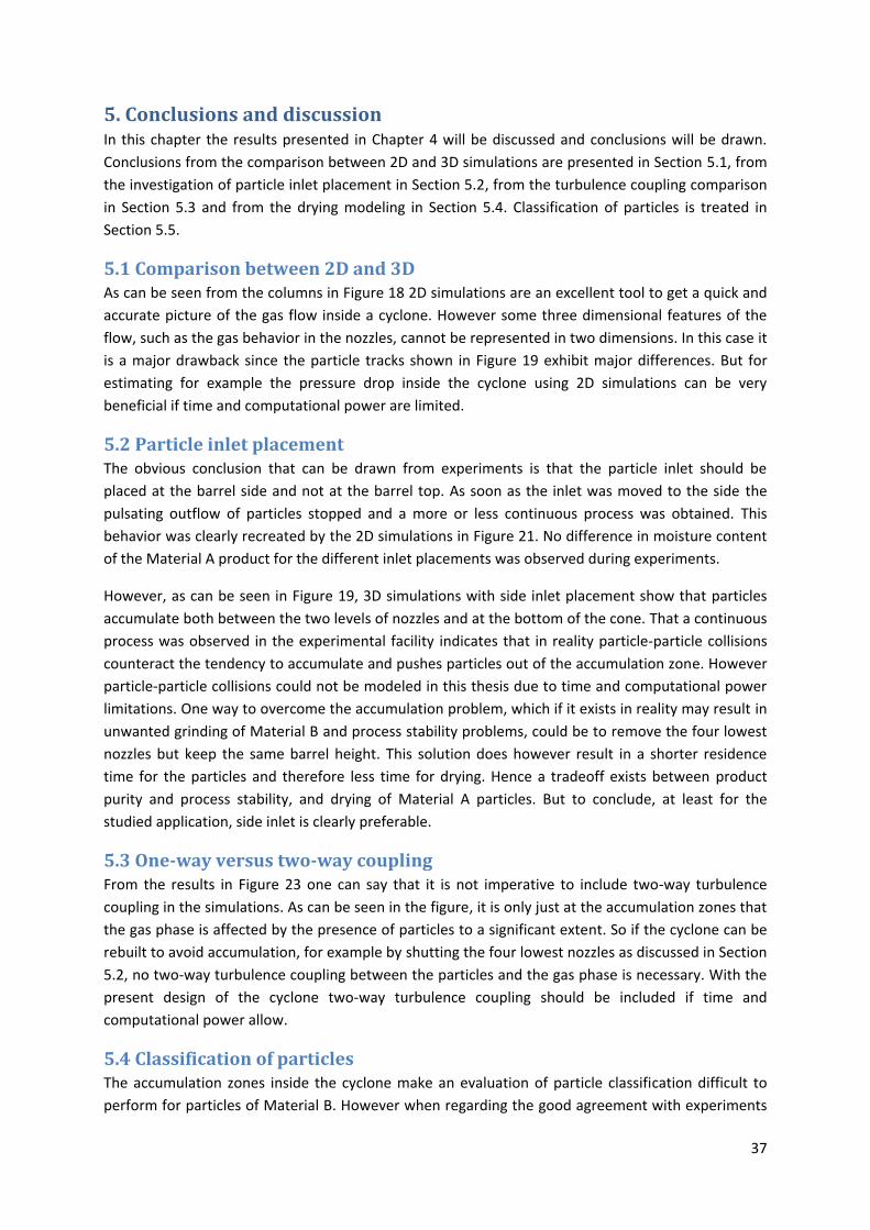
37
5. Conclusions and discussion In this chapter the results presented in Chapter 4 will be discussed and conclusions will be drawn.
Conclusions from the comparison between 2D and 3D simulations are presented in Section 5.1, from
the investigation of particle inlet placement in Section 5.2, from the turbulence coupling comparison
in Section 5.3 and from the drying modeling in Section 5.4. Classification of particles is treated in
Section 5.5.
5.1 Comparison between 2D and 3D As can be seen from the columns in Figure 18 2D simulations are an excellent tool to get a quick and
accurate picture of the gas flow inside a cyclone. However some three dimensional features of the
flow, such as the gas behavior in the nozzles, cannot be represented in two dimensions. In this case it
is a major drawback since the particle tracks shown in Figure 19 exhibit major differences. But for
estimating for example the pressure drop inside the cyclone using 2D simulations can be very
beneficial if time and computational power are limited.
5.2 Particle inlet placement The obvious conclusion that can be drawn from experiments is that the particle inlet should be
placed at the barrel side and not at the barrel top. As soon as the inlet was moved to the side the
pulsating outflow of particles stopped and a more or less continuous process was obtained. This
behavior was clearly recreated by the 2D simulations in Figure 21. No difference in moisture content
of the Material A product for the different inlet placements was observed during experiments.
However, as can be seen in Figure 19, 3D simulations with side inlet placement show that particles
accumulate both between the two levels of nozzles and at the bottom of the cone. That a continuous
process was observed in the experimental facility indicates that in reality particle-particle collisions
counteract the tendency to accumulate and pushes particles out of the accumulation zone. However
particle-particle collisions could not be modeled in this thesis due to time and computational power
limitations. One way to overcome the accumulation problem, which if it exists in reality may result in
unwanted grinding of Material B and process stability problems, could be to remove the four lowest
nozzles but keep the same barrel height. This solution does however result in a shorter residence
time for the particles and therefore less time for drying. Hence a tradeoff exists between product
purity and process stability, and drying of Material A particles. But to conclude, at least for the
studied application, side inlet is clearly preferable.
5.3 One-way versus two-way coupling From the results in Figure 23 one can say that it is not imperative to include two-way turbulence
coupling in the simulations. As can be seen in the figure, it is only just at the accumulation zones that
the gas phase is affected by the presence of particles to a significant extent. So if the cyclone can be
rebuilt to avoid accumulation, for example by shutting the four lowest nozzles as discussed in Section
5.2, no two-way turbulence coupling between the particles and the gas phase is necessary. With the
present design of the cyclone two-way turbulence coupling should be included if time and
computational power allow.
5.4 Classification of particles The accumulation zones inside the cyclone make an evaluation of particle classification difficult to
perform for particles of Material B. However when regarding the good agreement with experiments
38
for Material A particles it may be suspected that the results for Material B particles would be close to
the experimentally observed results, had particle-particle collisions been included. The studied
cyclone operates with much higher flow velocities than an ordinary cyclone which leads to low
pressure in the lower part of the cyclone due to strong rotational motion of the gas. The low
pressure will result in strong suction of air from the dust outlet into the cyclone. This suction of air is
the reason for the accumulation zone in the lower cone due to that the vertical gas velocities in this
region are higher than the terminal velocity of the particles.
Since the density of Material B particles is higher than for the wet Material A particles they are
subject to a larger centrifugal force which will keep them in the barrel with help from the upwards
flow from the lower nozzles as discussed in Section 4.1. The particles are injected with the same size
distribution as the bottom product observed in experiments and should hence exit through the dust
outlet. As described in Section 2.4.3.2, the reduction in tangential velocity associated with wall
collisions, particle-particle collisions forcing particles out of the accumulation zone and the gas flow
itself are responsible for particles leaving the accumulation zones. This may once again emphasize
the importance of including particle-particle collisions in the simulations to fully capture the particle
behavior. Also a two-way momentum coupling should result in lower gas velocities and hence
increased tendencies for the particles to fall down if it had it been included.
5.5 Drying of particles As mentioned in Section 4.4 the difference in particle moisture content observed in experiments and
in simulations is large. This is due to that the drying rate expression used in the UDF is fitted to drying
data obtained for the starting material. When the starting material collides with the cyclone wall the
particles will break. Smaller particles imply larger contact area between the particles and the gas
which will increase heat and mass transfer. In addition to this the internal transport resistance of the
particles will decrease meaning that the drying rate increases as well. As discussed in Section 2.4.3
some water may also leave the particles during breakage. Hence pulverization of the particles is the
most important phenomenon in the drying process of Material A.
It should be pointed out that the particle density and diameter changes in an incorrect fashion when
the drying rate UDF is utilized. In reality the density of the particle decrease during drying due to that
the water situated in the capillaries is replaced by air. In the simulations the density increases as
water is evaporated due to that the diameter decreases. The diameter decreases since Fluent views
the multicomponent particles as a droplet, as discussed in Section UDF. A second UDF, with the
purpose of keeping the particle diameter constant, was incorporated in the simulations. However the
second UDF overrode the drying rate UDF and no drying at all occurred. Hence the decision to
continue with the drying rate UDF and accept the erroneous values of particle density and diameter
was taken. Although it should be kept in mind that the reduction in particle density should make
larger particles follow the flow and exit at the gas outlet as top product.
39
6. Future work The suggested future work based on this thesis could include looking into the pulverization of
Material A more deeply. Population balance models could be simulated using CFD software as well.
The first simulations should include a one dimensional population balance over particle size to later
be augmented to a two dimensional population balance over both particle size and moisture content.
Also drying experiments on pulverized material should be run to obtain a drying rate expression that
better describes the situation in the cyclone. If possible, the problem of increasing particle density
and decreasing particle diameter during drying simulations could be addressed. If time and
computational power allows collisions between particles could also be taken into account. The
employed drying model should be validated against experiments since this was not possible due to
the pulverization of particles during experiments. An experiment should be conducted for which it is
made sure that no other drying phenomena than evaporation are taking place. This could be done
for example by running the cyclone with much lower gas velocities to prevent pulverization of
Material A.

40
Bibliography
[1] P. Atkins and L. Jones, Chemical Principles: The Quest for Insight, 4th ed., New York: W. H.
Freeman, 2008.
[2] A. Hoffmann and L. Stein, Gas Cyclones and Swirl Tubes: Principles, Design and Operation, 2nd
ed., New York: Springer-Verlag Berlin Heidelberg, 2008.
[3] Ansys, Inc., ANSYS FLUENT Theory guide, release 14.5, 2012.
[4] The Engineering ToolBox, "Gases - Explosive and Flammability Concentration Limits", [Online].
Available: http://www.engineeringtoolbox.com/explosive-concentration-limits-d_423.html.
[Accessed 10 March 2013].
[5] The Engineering ToolBox, "Fuels and Chemicals - Autoignition Temperatures", [Online].
Available: http://www.engineeringtoolbox.com/fuels-ignition-temperatures-d_171.html.
[Accessed 10 March 2013].
[6] SMHI, "Luftfuktighet", Sveriges meteorologiska och hydrologiska institut, 2 February 2012.
[Online]. Available: http://www.smhi.se/kunskapsbanken/meteorologi/luftfuktighet-1.3910.
[Accessed 10 February 2013].
[7] J. Seader and E. Henley, Separation Process Principles, 2nd ed., Hoboken, NJ: John Wiley & Sons,
Inc., 2006.
[8] M. Hidayat and A. Rasmuson, "Heat and Mass Transfer in U-Bend of a Pneumatic Conveying
Dryer", Chemical Engineering Research and Design, vol. 85, issue 3, pp. 307-319, 2007.
[9] J. Vaxelaire and P. Cézac, "Moisture Distribution in Activated Sludges: A Review", Water
Research, vol. 38, issue 9, pp. 2215-2230, 2004.
[10] H. Hwang, S.-H. Kim, T.-H. Kim, J.-K. Park and Y.-K. Cho, "Paper on a Disc: Balancing the Capillary-
Driven Flow with a Centrifugal Force", Lab on a Chip, vol. 11, issue 20, pp. 3404-3406, 2011.
[11] J. Welty, C. Wicks, R. Wilson and G. Rorrer, Fundamentals of Momentum, Heat and Mass
Transfer, 5th ed., Hoboken, NJ: John Wiley & Sons, Inc., 2008.
[12] R. Fitzpatrick, "Angle of Contact", The University of Texas at Austin, 27 April 2012. [Online].
Available: http://farside.ph.utexas.edu/teaching/336l/fluidhtml/node48.html. [Accessed 10
February 2013].
[13] M. Schwiebert and W. Leong, "Underfill Flow as a Viscous Flow Between Parallel Plates Driven by
Capillary Action", Components, Packaging and Manufacturing Technology, vol. 19, issue 2, pp.
133-137, 1996.
41
[14] E. A. Boucher, "Centrifugation of Porous Solids and Compacts Containing Imbibed or Capillary-
Condensed Fluid", Journal of Colloid and Interface Science, vol. 120, issue 1, pp. 289-291, 1987.
[15] J. Garcia-Corodero, L. Basabe-Desmonts, J. Ducrée and A. Ricco, "Liquid Recirculation in
Microfluidic Channels by the Interplay of Capillary and Centrifugal Forces", Microfluidics and
Nanofluidics, vol. 9, issue 4-5, pp. 695-703, 2010.
[16] C. Crowe, J. Schwartzkopf, M. Sommerfeld and Y. Tsuji, Multiphase Flows with Droplets and
Particles, 2nd ed., Boca Raton, FL: CRC Press, 2012.
[17] M. Mandø, "Turbulence Modulation by Non-spherical Particles", [Dissertation], Aalborg, Aalborg
University, 2009.
[18] J. Ye and M. Roco, "Particle Rotation in a Couette Flow", Physics of Fluids, vol. 4, issue 2, pp. 220-
224, 1991.
[19] J. Davis, "The Aerodynamics of Golf Balls", Journal of Applied Physics, vol. 20, issue 9, pp. 821-
828, 1949.
[20] Z. Zhang, H. Zhang and H. Ye, "Pressure-driven Flow in Parallel-plate Nanochannels", Applied
Physics Letters, vol. 95, issue 15, 2009.
[21] B. Andersson, R. Andersson, L. Håkansson, M. Mortensen, R. Sudiyo and B. van Wachem,
Computational Fluid Dynamics for Engineers, 8th ed., Gothenburg: Cambridge University Press,
2012.
[22] N. Moradian, D. Ting and S. Cheng, "The Effects of Freestream Turbulence on the Drag
Coefficient of a Sphere", Experimental Thermal and Fluid Science, vol. 33, issue 3, pp. 460-471,
2009.
[23] J. Elliot and C. Lira, Introductory Chemical Engineering Thermodynamics, Upper Saddle River:
Prentice Hall, 1999.
[24] K. Marsh, Recommended reference materials for the realization of physicochemical properties,
Oxford: Blackwell Scientific, 1987.
[25] A. Hoekstra, "Gas Flow Field and Collection Efficiency of Cyclone Separators", [Dissertation],
Delft, Delft University of Technology, 2000.
[26] S. Morsi and A. Alexander, "An Investigation of Particle Trajectories in Two-phase Flow Systems",
Journal of Fluid Mechanics, vol. 55, issue 2, pp. 193-208, 1972.
[27] CFD-online.com, "Fluent FAQ", [Online]. Available: http://www.cfd-
online.com/Wiki/Fluent_FAQ#My_UDF_won.27t_interpret_or_compile_-_what_is_wrong.3F.
[Accessed 8 June 2013].
42
[28] Ansys Support, Gothenburg, Communication by telephone and e-mail, 2013.
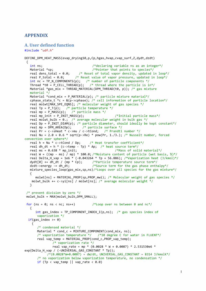
I
APPENDIX
A. User defined function #include "udf.h" DEFINE_DPM_HEAT_MASS(evap_drying10,p,Cp,hgas,hvap,cvap_surf,Z,dydt,dzdt) { int ns; /*declaring variable ns as an integer*/ Material *sp; /*Pointer that points to species*/ real dens_total = 0.0; /* Reset of total vapor density, updated in loop*/ real P_total = 0.0; /* Reset value of vapor pressure, updated in loop*/ int nc = TP_N_COMPONENTS(p); /* number of particle components */ Thread *t0 = P_CELL_THREAD(p); /* thread where the particle is in*/ Material *gas_mix = THREAD_MATERIAL(DPM_THREAD(t0, p)); /* gas mixture material */ Material *cond_mix = P_MATERIAL(p); /* particle mixture material*/ cphase_state_t *c = &(p->cphase); /* cell information of particle location*/ real molwt[MAX_SPE_EQNS]; /* molecular weight of gas species */ real Tp = P_T(p); /* particle temperature */ real mp = P_MASS(p); /* particle mass */ real mp_init = P_INIT_MASS(p); /*Initial particle mass*/ real molwt_bulk = 0.; /* average molecular weight in bulk gas */ real Dp = P_INIT_DIAM(p); /* particle diameter, should ideally be kept constant*/ real Ap = DPM_AREA(Dp); /* particle surface */ real Pr = c->sHeat * c->mu / c->tCond; /* Prandtl number */ real Nu = 2.0 + 0.6 * sqrt(p->Re) * pow(Pr, 1./3.); /* Nusselt number, forced convection over sphere*/ real h = Nu * c->tCond / Dp; /* Heat transfer coefficient*/ real dh_dt = h * (c->temp - Tp) * Ap; /* heat source term*/ real ms = 0.638 * mp_init; /*Mass of solid material*/ real W = ((mp - ms) / mp) * 100.0; /*Moisture content of particle (wet basis, %)*/ real Delta_H_vap = 1e6 * (-0.043264 * Tp + 56.886); /*Vaporization heat (J/kmol)*/ dydt[0] += dh_dt / (mp * Cp); /*Particle temperature source term*/ dzdt->energy -= dh_dt; /*Source term for the gas phase enthalpy*/ mixture_species_loop(gas_mix,sp,ns)/*Loops over all species for the gas mixture*/ { molwt[ns] = MATERIAL_PROP(sp,PROP_mwi); /* Molecular weight of gas species */ molwt_bulk += c->yi[ns] / molwt[ns]; /* average molecular weight */ } /* prevent division by zero */ molwt_bulk = MAX(molwt_bulk,DPM_SMALL); for (ns = 0; ns < nc; ns++) /*Loop over ns between 0 and nc*/ { int gas_index = TP_COMPONENT_INDEX_I(p,ns); /* gas species index of vaporization */ if(gas_index >= 0) { /* condensed material */ Material * cond_c = MIXTURE_COMPONENT(cond_mix, ns); /* vaporization temperature */ /*10 degree C for water in FLUENT*/ real vap_temp = MATERIAL_PROP(cond_c,PROP_vap_temp); /* vaporization rate */ real vap_rate = mp * (0.0028 * W + 0.0087) * 2.531530e6 * exp(Delta_H_vap / (-UNIVERSAL_GAS_CONSTANT * Tp)); /*(0.0028*W+0.0087) = dW/dt, UNIVERSAL_GAS_CONSTANT = 8314 J/kmolK*/ /* no vaporization below vaporization temperature, no condensation */ if (Tp < vap_temp || vap_rate < 0.0)
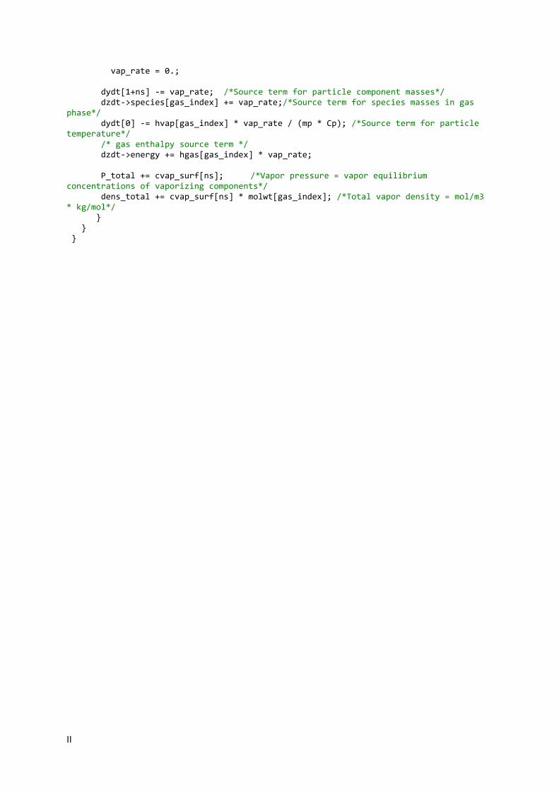
II
vap_rate = 0.; dydt[1+ns] -= vap_rate; /*Source term for particle component masses*/ dzdt->species[gas_index] += vap_rate;/*Source term for species masses in gas phase*/ dydt[0] -= hvap[gas_index] * vap_rate / (mp * Cp); /*Source term for particle temperature*/ /* gas enthalpy source term */ dzdt->energy += hgas[gas_index] * vap_rate; P_total += cvap_surf[ns]; /*Vapor pressure = vapor equilibrium concentrations of vaporizing components*/ dens_total += cvap_surf[ns] * molwt[gas_index]; /*Total vapor density = mol/m3 * kg/mol*/ } } }
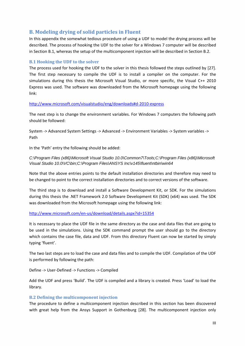
III
B. Modeling drying of solid particles in Fluent In this appendix the somewhat tedious procedure of using a UDF to model the drying process will be
described. The process of hooking the UDF to the solver for a Windows 7 computer will be described
in Section B.1, whereas the setup of the multicomponent injection will be described in Section B.2.
B.1 Hooking the UDF to the solver
The process used for hooking the UDF to the solver in this thesis followed the steps outlined by [27].
The first step necessary to compile the UDF is to install a compiler on the computer. For the
simulations during this thesis the Microsoft Visual Studio, or more specific, the Visual C++ 2010
Express was used. The software was downloaded from the Microsoft homepage using the following
link:
http://www.microsoft.com/visualstudio/eng/downloads#d-2010-express
The next step is to change the environment variables. For Windows 7 computers the following path
should be followed:
System -> Advanced System Settings -> Advanced -> Environment Variables -> System variables ->
Path
In the ‘Path’ entry the following should be added:
C:\Program Files (x86)\Microsoft Visual Studio 10.0\Common7\Tools;C:\Program Files (x86)\Microsoft
Visual Studio 10.0\VC\bin;C:\Program Files\ANSYS Inc\v145\fluent\ntbin\win64
Note that the above entries points to the default installation directories and therefore may need to
be changed to point to the correct installation directories and to correct versions of the software.
The third step is to download and install a Software Development Kit, or SDK. For the simulations
during this thesis the .NET Framework 2.0 Software Development Kit (SDK) (x64) was used. The SDK
was downloaded from the Microsoft homepage using the following link:
http://www.microsoft.com/en-us/download/details.aspx?id=15354
It is necessary to place the UDF file in the same directory as the case and data files that are going to
be used in the simulations. Using the SDK command prompt the user should go to the directory
which contains the case file, data and UDF. From this directory Fluent can now be started by simply
typing ‘fluent’.
The two last steps are to load the case and data files and to compile the UDF. Compilation of the UDF
is performed by following the path:
Define -> User-Defined -> Functions -> Compiled
Add the UDF and press ‘Build’. The UDF is compiled and a library is created. Press ‘Load’ to load the
library.
B.2 Defining the multicomponent injection
The procedure to define a multicomponent injection described in this section has been discovered
with great help from the Ansys Support in Gothenburg [28]. The multicomponent injection only
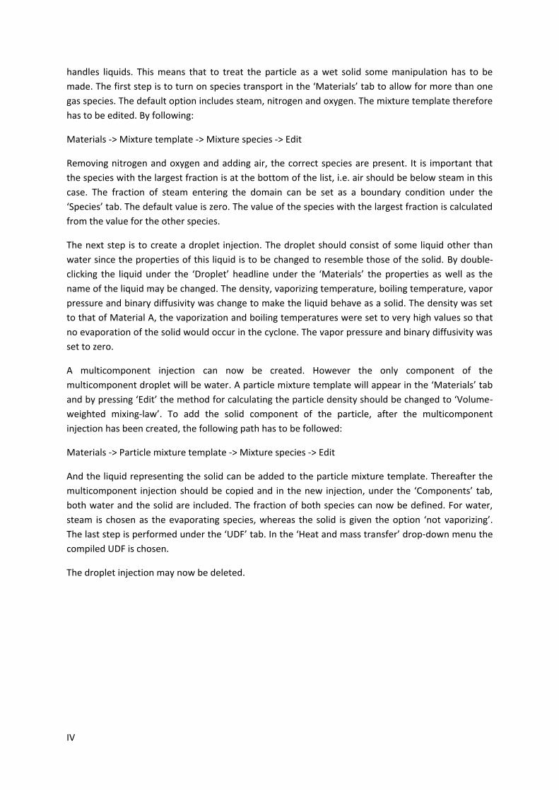
IV
handles liquids. This means that to treat the particle as a wet solid some manipulation has to be
made. The first step is to turn on species transport in the ‘Materials’ tab to allow for more than one
gas species. The default option includes steam, nitrogen and oxygen. The mixture template therefore
has to be edited. By following:
Materials -> Mixture template -> Mixture species -> Edit
Removing nitrogen and oxygen and adding air, the correct species are present. It is important that
the species with the largest fraction is at the bottom of the list, i.e. air should be below steam in this
case. The fraction of steam entering the domain can be set as a boundary condition under the
‘Species’ tab. The default value is zero. The value of the species with the largest fraction is calculated
from the value for the other species.
The next step is to create a droplet injection. The droplet should consist of some liquid other than
water since the properties of this liquid is to be changed to resemble those of the solid. By double-
clicking the liquid under the ‘Droplet’ headline under the ‘Materials’ the properties as well as the
name of the liquid may be changed. The density, vaporizing temperature, boiling temperature, vapor
pressure and binary diffusivity was change to make the liquid behave as a solid. The density was set
to that of Material A, the vaporization and boiling temperatures were set to very high values so that
no evaporation of the solid would occur in the cyclone. The vapor pressure and binary diffusivity was
set to zero.
A multicomponent injection can now be created. However the only component of the
multicomponent droplet will be water. A particle mixture template will appear in the ‘Materials’ tab
and by pressing ‘Edit’ the method for calculating the particle density should be changed to ‘Volume-
weighted mixing-law’. To add the solid component of the particle, after the multicomponent
injection has been created, the following path has to be followed:
Materials -> Particle mixture template -> Mixture species -> Edit
And the liquid representing the solid can be added to the particle mixture template. Thereafter the
multicomponent injection should be copied and in the new injection, under the ‘Components’ tab,
both water and the solid are included. The fraction of both species can now be defined. For water,
steam is chosen as the evaporating species, whereas the solid is given the option ‘not vaporizing’.
The last step is performed under the ‘UDF’ tab. In the ‘Heat and mass transfer’ drop-down menu the
compiled UDF is chosen.
The droplet injection may now be deleted.
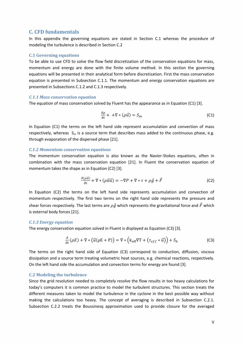
V
C. CFD fundamentals In this appendix the governing equations are stated in Section C.1 whereas the procedure of
modeling the turbulence is described in Section C.2
C.1 Governing equations
To be able to use CFD to solve the flow field discretization of the conservation equations for mass,
momentum and energy are done with the finite volume method. In this section the governing
equations will be presented in their analytical form before discretization. First the mass conservation
equation is presented in Subsection C.1.1. The momentum and energy conservation equations are
presented in Subsections C.1.2 and C.1.3 respectively.
C.1.1 Mass conservation equation
The equation of mass conservation solved by Fluent has the appearance as in Equation (C1) [3].
( ⃗ ) (C1)
In Equation (C1) the terms on the left hand side represent accumulation and convection of mass
respectively, whereas Sm is a source term that describes mass added to the continuous phase, e.g.
through evaporation of the dispersed phase [21].
C.1.2 Momentum conservation equations
The momentum conservation equation is also known as the Navier-Stokes equations, often in
combination with the mass conservation equation [21]. In Fluent the conservation equation of
momentum takes the shape as in Equation (C2) [3].
( ⃗⃗ )
( ⃗ ⃗ ) (C2)
In Equation (C2) the terms on the left hand side represents accumulation and convection of
momentum respectively. The first two terms on the right hand side represents the pressure and
shear forces respectively. The last terms are which represents the gravitational force and which
is external body forces [21].
C.1.3 Energy equation
The energy conservation equation solved in Fluent is displayed as Equation (C3) [3].
( ) ( ⃗ ( )) ( ( ⃗ )) (C3)
The terms on the right hand side of Equation (C3) correspond to conduction, diffusion, viscous
dissipation and a source term treating volumetric heat sources, e.g. chemical reactions, respectively.
On the left hand side the accumulation and convection terms for energy are found [3].
C.2 Modeling the turbulence
Since the grid resolution needed to completely resolve the flow results in too heavy calculations for
today’s computers it is common practice to model the turbulent structures. This section treats the
different measures taken to model the turbulence in the cyclone in the best possible way without
making the calculations too heavy. The concept of averaging is described in Subsection C.2.1.
Subsection C.2.2 treats the Boussinesq approximation used to provide closure for the averaged
VI
governing equations. The employed turbulence model is described in Subsection C.2.3, whereas the
treatment of the near-wall turbulent boundary layer is treated in Subsection C.2.4.
C.2.1 Reynolds averaging
Due to limitation of computational power it is not possible to solve the instantaneous governing
equations defined in Section C.1. It is therefore convenient to decompose the variables in an
averaged and a fluctuating part. During simulation only the averaged part is solved for whereas the
fluctuating part is modeled. This is known as Reynolds-decomposition and can, for a variable be
written as Equation (C4) [21].
(C4)
In Equation (C4) is the averaged part and is the fluctuating part, often regarded as representing
the turbulence. For incompressible flow only the velocities and the pressure is decomposed
according to Equation (C4). If the flow is compressible the density has to be decomposed in a similar
way [21].
After inserting the averaged variables into the governing equations Equation (C1) and (C2) take the
form of Equations (C5) and (C6) [3], [21].
( ) (C5)
( )
( )
[ (
)]
( ̅̅ ̅̅ ̅̅ ̅ ) (C6)
Equations (C5) and (C6) are known as the Reynolds-averaged Navier-Stokes, or RANS, equations [21].
C.2.2 The Boussinesq approximation
When the governing equations are written as in Section C.2.1 they are unclosed. This means that the
number of variables is greater than the number of equations. The problem arises because of the last
term in Equation (C6), namely the Reynolds stresses . Therefore it is of importance to model
the Reynolds stresses. A commonly employed equation is the Boussinesq approximation which can
be written as Equation (C8) [21].
(
)
(C8)
From Equation (C8) it can be seen that the assumption behind the Boussinesq approximation is that
the Reynolds stresses are proportional to the gradients of the mean velocity. In Equation (C8) is
the turbulent viscosity, which in turn can be written as Equation (C9) [21].
(C9)
In Equation (C9) is the energy-dissipation rate. The turbulent kinetic energy k and the energy-
dissipation rate are two new unknowns. Closure for these two variables can be obtained by the use
of transport equations as is frequently done in two-equation turbulence models [21].
VII
C.2.3 The RNG k-epsilon turbulence model
Some turbulence models, such as the Reynolds stress model, or RSM, does not use the Boussinesq
approximation but instead solve transport equations directly for the Reynolds stresses. Since this
requires less modeling the results are generally more accurate. However this comes at the price of 9
additional transport equations which puts high demands on the available computational power. The
RSM model is significantly more computational expensive than a two-equation model such as the
renormalization group, or RNG, k- model [21]. According to Hoekstra [25] the RNG k- model is
inferior to the RSM model when it comes to model the flow inside a cyclone separator due to that it
is not able to capture the axial velocity profiles compared to experiments whereas the RSM is.
However the RNG k- model was used in the simulations in this thesis since the assessment that this
model would give a good compromise between accuracy and computational cost was made.
The closed transport equation for the turbulent kinetic energy is written as Equation (C10) in the
RNG k- model [21].
[(
)
]
[(
)
] (C10)
The terms on the left hand side of Equation (C10) denote accumulation and convection of turbulent
energy respectively. The terms on the right hand side describe production of turbulent energy as
large eddies extract energy from the mean flow, dissipation of turbulent energy into heat, molecular
diffusion of turbulent energy and turbulent transport of energy due to velocity and pressure
fluctuations respectively. The closed transport equation for is written as Equation (C11) [21].
[(
)
]
[(
)
] (C11)
The terms on the left hand side of Equation (C11) describe the accumulation and convection of
energy-dissipation respectively. On the right hand side the first three terms represent production,
dissipation and diffusion of energy-dissipation respectively. The last term on the right hand side is a
source term that is modeled as Equation (C12) [21].
(
√ )
(
√
)
( (
√ )
)
(C12)
In Equation (C12) Sij is the strain-rate tensor whereas , and are constants. This source term is
unique for the RNG k- model and results in less destruction of energy-dissipation in this model
than in other two-equation models. If less energy-dissipation is destroyed the energy-dissipation will
increase and as a consequence the turbulent kinetic energy will decrease. As can be seen in Equation
(C9) this will decrease the turbulent viscosity and hence less turbulent energy will be dissipated into
heat. Hence the RNG k- model is less dissipative than other two-equation models that do not
include the source term defined in Equation (C12), e.g. the standard k- model. Therefore, the RNG
k- model is better suited for flows which involve swirls [21]. Since swirling flow is a fundamental
feature of a cyclone the RNG k- model was chosen for the simulations.
VIII
C.2.4 Enhanced wall treatment
The turbulence model described in Section C.2.3 is not able to describe the behavior of the
turbulence close to the walls. Therefore the need to use wall functions arises to model the behavior
in the boundary layers. Wall boundary layers can be divided into an inner and an outer region, where
the inner region in turn can be divided into three additional regions. The region closest to the wall is
the viscous sub-layer, where viscosity damps out turbulence. Farthest from the wall in the inner
region is the fully turbulent sub-layer, where shear forces dominates viscous forces. Between these
two sub-layers a buffer sub-layer exists [21].
When the enhanced wall treatment is used to model the near-wall flow, grids of varying resolution
can be handled with satisfying results. This is because a combination of the two-layer zonal model
used for fine grids and enhanced wall functions used for coarser grids is employed [3]. The enhanced
wall treatment was used for the simulations in this thesis.
In the two-layer zonal model the computational domain is divided into two different regions, namely
the viscosity-affected region and the fully turbulent region. The distinction between the two regions
is made based on a wall-distance Reynolds number, expressed as Equation (C13) [3], [21].
√
(C13)
In Equation (C13) y is the distance to the nearest wall. If the wall-distance based Reynolds number is
below 200 the region is said to be viscosity-affected. If this is the case, a transport equation is solved
for the turbulent kinetic energy k whereas an algebraic expression is used to solve for the energy-
dissipation rate . Outside the viscosity-affected region, in the turbulent region, is solved for with a
transport equation. This means that a turbulence model is applied as usual, in this case the RNG k-
model. To facilitate convergence a blending factor, defined as zero at the wall and unity far from the
wall, is used to match the values of the turbulent viscosity obtained at the boundary between the
turbulent and the viscosity-affected region [3], [21].
The difference between enhanced and standard wall functions is that the enhanced wall functions
use a blending function to blend the laws-of-the-wall in the laminar and the fully turbulent sub-
region. This enables the formulation of a single law-of-the-wall valid for the whole near-wall region.
Therefore no lower boundary for the dimensionless wall distance y+ exists when using the enhanced
wall treatment which facilitates the mesh construction and is the reason why enhanced wall-
treatment was used in the simulations in this thesis [3].