3d multiphase numerical modelling for turbidity current flows

3

3D Multiphase Numerical Modelling for Turbidity Current Flows

A. Georgoulas, P. Angelidis, K. Kopasakis and N. Kotsovinos Democritus University of Thrace, Xanthi

Greece

1. Introduction

Gravity or density currents constitute a large class of natural flows that are generated and driven by the density difference between two or even more fluids. The density difference between two fluids usually arises due to differences in temperature or salinity, but it can also arise due to the presence of suspended solid particles. These particulate currents, in the case of sediment laden water that enters a water basin, are classified according to the density difference with the ambient fluid into three major categories: a) hypopycnal currents, when the density of the sediment laden water is lower than that of the receiving water basin, b) homopycnal currents, when the density of the sediment laden water is almost equal to that of the receiving water basin, and c) hyperpycnal currents when their density is much greater than that of the receiving water body (Mulder & Alexander, 2001). In the case of floods, the suspended sediment concentration of river water rises to a great extent. Hence, the river plunges to the bottom of the receiving basin and forms a hyperpycnal plume which is also known as turbidity current. Such flows are usually formed at river mouths in oceans, lakes or reservoirs, and can travel remarkable distances transferring, eroding and depositing large amounts of suspended sediments (Mulder & Alexander, 2001).

Turbidity currents are very difficult to be observed and studied in the field. This is due to their rare and unexpected occurrence nature, as they are usually formed during floods. Therefore, field investigations are usually limited to the study of the deposits originating from such currents. The anatomy of deposits originating from turbidity currents can be studied on a large scale, in order to identify the various depositional elements such as lobes, levees and submarine channels (Janbu et al., 2009). Furthermore, considerable research on the morphology of turbiditic systems and general deep-marine depositions is being increasingly done with the use of 3D seismic sections (Posamentier & Kolla, 2003; Saller et al., 2006).

On the other hand, scaled laboratory experiments constitute an alternative and widely used method for simulating and studying the dynamics of turbidity currents. Many researchers have been focused in the study of the flow dynamics, depositional and erosional characteristics of laboratory turbidity currents, using scaled experimental models (Britter & Linden, 1980; Lovell, 1971; Garcia & Parker, 1989; Simpson & Britter, 1979). Advances in experimental technology in the last decades have increased the existing knowledge from

www.intechopen.com

Numerical Modelling

46

macroscopic and qualitative descriptions of turbidity current behaviour and deposits, to detailed, quantitative results relating to the actual flow characteristics, such as the velocity, concentration as well as the turbulence structure of such flows (Baas et al., 2004; Garcia, 1994; Gladstone et al., 1998; Kneller et al., 1997).

Mathematical and numerical models when properly designed and tested against field or laboratory data, can provide significant knowledge for turbidity current dynamics as well as for erosional and depositional characteristics. Up to present, there are various numerical investigations dealing with turbidity current dynamics and flow characteristics, providing valuable results regarding these complex phenomena. The characteristics of a gravity-current head have been studied by (Hartel et al., 2000), using 3D Direct Numerical Simulations (DNS) of flow fronts in the lock-exchange configuration. (Kassem & Imran, 2001) present a 2D numerical approach for investigating the transformation of a plunging river flow into a turbidity current. In the work of (Heimsund et al., 2002) a computational, 3D, fluid-dynamics model for sediment transport, erosion and deposition by turbidity currents has been constructed using the CFD (Computational Fluid Dynamics) software Flow-3D. Another 3D numerical model using the CFX-4 code was developed, in order to simulate turbidity currents in Lake Lugano (Switzerland), in the work of (Lavelli et al., 2002). (Necker et al., 2002) presented 2D and 3D Direct Numerical Simulations of particle-driven gravity currents, placing special emphasis on the sedimentation of particles, and the influence of particle settling on the flow dynamics. (Cantero et al., 2003) present two and three-dimensional CFD simulations of a discontinuous density current, using a stabilized equal-order finite element method. A comparative study on the convergence of CFD commercial codes, when simulating dense underflows is presented by (Bombardelli et al., 2004). Two codes are used for the proposed simulations: the first one is a comprehensive finite-element platform, whereas the other one is a commercial code. The lateral development of density-driven flow in a subaqueous channel is studied using a 3D numerical model, in the work of (Imran et al., 2004). The conditions under which turbidity currents may become self-sustaining through particle entrainment are investigated in the work of (Blanchette et al., 2005), using 2D Direct Numerical Simulations of resuspending gravity currents. A numerical model of turbidity currents with a deforming bottom boundary, that predicts the vertical structure of the flow velocity and concentration as well as the change in the bed level, due to erosion and deposition of suspended sediment, is developed in the work of (Huang et al., 2005). Lock-exchange gravity current flows, produced by the instantaneous release of a heavy fluid, are investigated by means of 2D Large-Eddy Simulation (LES) in the work of (Ooi et al., 2007). A numerical simulation of

turbidity current using the fv2 turbulence model is carried out in the work of

(Mehdizadeh et al., 2008). (Cantero et al., 2008a), perform 2D Direct Numerical Simulations in order to investigate the effect of particle inertia on the dynamics of particulate gravity currents. They introduce an Eulerian-Eulerian formulation for gravity currents driven by inertial particles. 3D Direct Numerical Simulations of planar gravity currents have been conducted with the objective of identifying, visualizing and describing turbulent structures and their influence on flow dynamics, in the work of (Cantero et al., 2008b). The investigation of the effect of initial aspect ratio on the flow characteristics of suspension gravity currents as well as the diffusion of the turbidity under the presence of a turbidity fence is carried out in the work of (Singh, 2008), using 3D Large Eddy Simulations.

www.intechopen.com


47

Most of these previous CFD-based investigations treat turbidity currents with a quasi-single-phase approach, since the transport of sediment particles is taken into account through an advection-diffusion equation for sediment concentration. The present chapter aims to present the validity, usefulness and applicability of a three-dimensional, “uncommon”, CFD-based, multiphase numerical approach for the simulation and study of the hydrodynamic and depositional characteristics of turbidity currents that are usually formed at river outflows in the sea, lakes and reservoirs. The numerical model is based in a multiphase modification of the Reynolds Averaged Navier-Stokes Equations (RANS). Turbulence closure is achieved through the application of the RNG (Renormalization-Group) k-ε turbulence model. The calculations of the model are performed using the robust CFD solver FLUENT. The proposed numerical model for the simulation of turbidity current hydrodynamics was firstly introduced in the work of (Georgoulas et al., 2010).

In the present section of the chapter (Section 1) a brief introduction on turbidity currents and a literature review on field, experimental and numerical studies are conducted while the main aim of the chapter is also stated. In Section 2 the theoretical background of the proposed numerical approach is presented and discussed in detail, while in Section 3 some main validation results are presented (Georgoulas et al., 2010). Section 4 presents the results of a laboratory-scale (Georgoulas, 2010) and a field scale (Georgoulas et al, 2009) application of the numerical approach. Finally, in Section 5 the main concussions that are withdrawn from the present chapter are summarized.

2. Numerical model description

2.1 Overview

Turbidity current flows can be characterized as multiphase flow systems, since they consist of a primary fluid phase (water) and secondary granular phases (suspended sediment classes) dispersed into the primary phase. Therefore, turbidity currents can be modeled through the application of suitable multiphase numerical models. Since, the particulate loading of turbidity currents may vary from small to considerably large values, an Eulerian-Eulerian multiphase numerical approach is considered to be more appropriate, as it can handle a wider range of particle volume fractions than an Eulerian-Lagrangian approach (maximum particles volume fraction of 10-12%). FLUENT provides various multiphase models that are based in the Eulerian-Eulerian approach. The “Eulerian” model that has been selected for the numerical approach that is presented in the present chapter, may require more computational effort, but it can handle a wider range of particulate loading values and is more accurate than the other available multiphase models in FLUENT. In this multiphase model, the different phases are treated mathematically as interpenetrating continua and therefore the concept of phasic volume fraction is introduced, where the volume fraction of each phase is assumed to be a continuous function of space and time. The sum of the volume fractions of the various phases is equal to unity. An accordingly modified set of momentum and continuity equations for each phase is solved. Pressure and inter-phase exchange coefficients are used in order to achieve coupling for these equations (Georgoulas et al., 2010).

The motion of the suspended sediment particles within a turbidity current as well as the motion generated in the ambient fluid are of highly turbulent nature. In order to account for

www.intechopen.com

Numerical Modelling

48

the effect of turbulence in the numerical simulations of the present investigation, the instantaneous governing equations are not applied directly but they are ensemble-averaged, converting turbulent fluctuations into Reynolds stresses, which represent the effects of turbulence. This averaging procedure for the numerical simulation of turbulent flows is known as RANS (Reynolds-averaged Navier-Stokes equations). The averaged governing equations contain additional unknown variables, and turbulence models are needed to determine these variables in terms of known quantities. Therefore, with this averaging approach the turbulence is modeled and only the unsteady, mean flow structures that are primarily larger than the turbulent eddies are resolved. This is the main difference with the other two widely used numerical approaches for turbulent flows, known as DNS (Direct Numerical Simulation) and LES (Large Eddy Simulation). In DNS, the Navier-Stokes equations are applied and solved directly without the application of a turbulence model, resolving the whole range of turbulent eddies. In LES on the other hand, large eddies are resolved directly, while small eddies are modeled. DNS and LES may provide detailed information on turbidity current flows but their major disadvantage is that their application is limited due to large computational requirements. On the other hand, RANS may not provide detailed information from a microscopic point of view, but is quite accurate and attractive for modeling large scale, three dimensional flows of practical engineering interest due to the relatively low computational cost (Georgoulas et al., 2010).

In the numerical approach presented here, the Renormalization-group (RNG) k-ε model is applied for turbulence closure. This model was derived using a rigorous statistical technique, the renormalization group theory. The basic form of the RNG k-ε model is similar to the standard k-ε model, but it includes a number of refinements, rendering it more appropriate for the case of turbidity currents, as it is more accurate for swirling flows and rapidly strained flows and also accounts for low Reynolds number effects. Moreover, it provides an analytical formula for the calculation of the turbulent Prandtl numbers. At this point it should be mentioned that in the present numerical approach, the RNG k-ε model is also modified accordingly in order to simultaneously account for the primary (continuous) phase and the secondary (dispersed) phases of the simulated flows. This modification in FLUENT is based on a number of assumptions. In more detail, turbulent predictions for the continuous phase are obtained using the RNG k-ε model, supplemented with extra terms that include the interphase turbulent momentum transfer. Predictions for turbulence quantities for the dispersed phases are obtained using the Tchen theory of dispersion of discrete particles by homogeneous turbulence. Interphase turbulent momentum transfer is also assumed, in order to take into account the dispersion of the secondary phases transported by the turbulent fluid motion. Finally, a phase-weighted averaging process is assumed, so that no volume fraction fluctuations are introduced into the continuity equations (Georgoulas et al., 2010).

2.2 Governing equations

The volume of phase q, Vq is defined by the following relationship (ANSYS FLUENT Documentation, 2010):

qqV

dVV (1)

www.intechopen.com


49

where,

n

qq 1

1

(2)

and αq is the volume fraction of phase q.

The effective density of phase q is:

q q q (3)

where ρq is the physical density of phase q.

The continuity, the fluid-fluid, and fluid-solid momentum equations that are actually solved by the model are described by equations (4), (5) and (6) respectively, for the general case of a n-phase flow consisting of granular and non-granular secondary phases (ANSYS FLUENT Documentation, 2010):

qq q q qrq t

1( ) ( ) 0

(4)

q qq q q q q q q q q

n

q lift q vm qp qpqp

p gt

K F F F, ,1

( ) ( )

( ( )) ( )

(5)

s ss s s s s s s s s s

N

s lift s vm sl slsl

p p gt

K F F F, ,

1

( ) ( )

( ( )) ( )

(6)

where ρrq is the phase reference density, or the volume averaged density of the qth phase in

the solution domain, q is the velocity of phase q,

p is the velocity of phase p, p is the

pressure shared by all phases, q is the qth phase stress-strain tensor, g

is the gravitational

acceleration, Kpq is the interphase momentum exchange coefficient, qF

is an external body

force, lift qF ,

is a lift force and vm qF ,

is a virtual mass force. Kls = Ksl is the momentum

exchange coefficient between fluid phase l and solid phase s and N is the total number of

phases. The stress-strain tensors q and

s are calculated by the following relationships:

Tq q q qq q q q q I

2

3

(7)

www.intechopen.com

Numerical Modelling

50

Ts s s ss s s s s I

2

3

(8)

where, ┤q and ┤s are the shear viscosities of phases q and s, ┣q and ┣s are the bulk viscosities

of phases q and s, and I is the identity tensor.

The momentum exchange between the various phases involved in a multiphase flow is based in the value of the interphase exchange coefficients. Therefore, these coefficients are very important for the simulation of granular multiphase flows, as turbidity currents. In the numerical approach presented here, the fluid-solid momentum exchange coefficient, between the ambient water (primary phase) and the suspended sediment particles (secondary phase) is calculated using the Syamlal-O'Brien model, which is based on measurements of the terminal velocities of particles in fluidized or settling beds. This model was selected, as a series of trial numerical runs indicated that this gives the best results, in comparison with corresponding experimental measurements, for the case of turbidity currents (Georgoulas et al., 2010). As it can be seen from Equation (6), in the case of granular flows, in the regime where the solids volume fraction is less than its maximum allowed value, a solids pressure is calculated independently and used for the pressure gradient term

(s

p ), in the fluid-solid momentum equation. This solids pressure is composed of a kinetic

term as well as a second term due to particle collisions and is calculated using the following relationship (ANSYS FLUENT Documentation, 2010):

s s s s s ss s ss sp e g20,2 (1 ) (9)

where ess is the coefficient of restitution for particle collisions, g0,ss is the radial distribution function, and Θs is the granular temperature which is proportional to the kinetic energy of the fluctuating particle motion. Trial numerical simulations indicated that the solids pressure is significant at various regions and stages of turbidity current flows (Georgoulas et al., 2010).

The effect of lift forces in the secondary phase solid particles is also taken into account. These lift forces act on particles mainly due to velocity gradients in the primary-phase flow field. The lift force will be more significant for larger particles. A main assumption is that the particle diameter is much smaller than the interparticle spacing. Hence, the inclusion of lift forces is not appropriate for closely packed particles or for very small particles. The lift force acting on a secondary phase p in a primary phase q is calculated in FLUENT, using the following equation (ANSYS FLUENT Documentation, 2010):

lift q p qL q pF C ( ) ( ) (10)

where CL is the lift coefficient. For the turbidity current cases that are presented in the present chapter, values of the lift coefficient ranging from 0.1 to 0.5 give the best results in comparison with corresponding experimental measurements (Georgoulas et al., 2010).

The virtual mass force is usually significant, in cases where the secondary phase density is much smaller than the primary phase density (ANSYS FLUENT Documentation, 2010). For example, the virtual mass force would be significant in the case of air bubbles moving

www.intechopen.com


51

through water, as in this case the density of air is much smaller than the density of the ambient water and the added mass (by the surrounding water) in the air bubbles would be much larger than their own mass. In all of the turbidity current cases considered in the present chapter, the secondary phase density (solid particles) is larger than the primary phase density (fresh water) and therefore the virtual mass force is not taken into consideration.

The general transport equations for the turbulence kinetic energy k and the turbulence dissipation rate ε, of the RNG k-ε turbulence model, can be described by equations (11) and (12) respectively (ANSYS FLUENT Documentation, 2010):

i k eff k bi j j

kk ku G G

t x x x( ) ( ) (11)

i eff

i j j

k b

ut x x x

C G C G C Rk k

2

1 3 2

( ) ( )

( )

(12)

where u represents velocity, ρ is the local mixture density, Gk is the generation of turbulence kinetic energy due to mean velocity gradients, Gb is the generation of turbulence kinetic energy due to buoyancy, αk and αε are the inverse effective Prandtl numbers for k and ε respectively, ┤eff is the effective viscosity and C1ε, C2ε and C3ε are turbulence model constants. The term Rε in the ε equation accounts for the effects of rapid strain and streamline curvature (ANSYS FLUENT Documentation, 2010).

2.3 Solution procedure

The governing equations in the proposed multiphase numerical approach are solved sequentially, using the control-volume method. Hence, the equations are integrated about each control-volume, yielding discrete equations for the conservation of each quantity. An implicit formulation is used, in order for the discretized equations to be converted to linear equations for the dependent variables in every computational cell. Further details regarding the solution procedure can be found at (ANSYS FLUENT Documentation, 2010).

2.4 Boundary conditions

At inlets, a velocity-inlet boundary condition is used. With this type of boundary condition, a uniform distribution of all the dependent variables is prescribed at the face representing the sediment laden water inflow. In more detail, the velocity magnitudes of the primary and secondary phases with directions normal to the inlet face are specified, assuming constant, uniform values. Moreover, the volume fractions of the secondary phases at the inlet are also specified.

For the outlets, a pressure-outlet boundary condition is applied. Using this type of boundary condition, all flow quantities at the outlets are extrapolated from the flow in the interior domain. A set of "backflow'' conditions can be also specified, allowing reverse direction flow at the pressure outlet boundary during the solution process. In other words, this type of

www.intechopen.com

Numerical Modelling

52

outlet condition serves as an open flow boundary, allowing the flow to freely exit or enter the computational domain during the calculations.

At the free ambient water surfaces, a symmetry boundary condition is used, which is typically well above the generated turbidity currents. Thus, there are neither convective nor diffusive fluxes across the top surface. This type of free surface boundary condition has also been used by other researchers in literature (Imran et al., 2004; Huang et al., 2005) for the case of turbidity currents. (Farrell & Stefan, 1986) have found that for a plunging reservoir flow, the relative error that can be introduced by this approximation of the free surface, is of the order of 10-3 and does not influence the velocity field.

The solid boundaries are specified as stationary walls with a no-slip shear condition. Turbulent flows are significantly affected by the presence of walls. Very close to the wall, viscous damping and kinematic blocking reduce the tangential and normal velocity fluctuations respectively. However, in the outer part of the near wall region, the turbulence is rapidly augmented by the production of turbulent kinetic energy due to the relatively large gradients in mean velocity. In FLUENT, there are two different approaches for modeling the near wall region. In the first approach, the viscous sub-layer and the buffer sub-layer are not resolved. Instead, semi-empirical formulas known as "wall functions" (e.g. “standard wall functions”) are used in order to link the viscosity affected sub-layers between the wall and the fully-turbulent region. In the second approach, known as "near-wall modeling" approach (e.g. “enhanced wall treatment), the turbulence models are modified in order for the viscosity affected near-wall regions to be resolved with a computational mesh all the way to the wall. However, the computational mesh must be significantly fine in these regions. This approach may require more computational effort, but it gives more accurate predictions at the near-wall region of the computational domain. Therefore, wall functions should only be used in cases where the complexity and size of the computational domain as well as the available computational resources, do not allow the construction of very fine meshes at the near-wall regions (ANSYS FLUENT Documentation, 2010).

3. Numerical model validation

A detailed verification of the proposed numerical model is conducted in the work of (Georgoulas et al., 2010), where two different series of published laboratory experiments on turbidity currents, conducted by (Gladstone et al., 1998) and (Baas et al., 2004) are reproduced numerically, and the results are compared aiming to evaluate how realistic and reliable the numerical simulations of the proposed model are. The first series of laboratory experiments (Gladstone et al., 1998) consist of fixed-volume lock-gate releases of dilute mixtures containing two different sizes of suspended silicon carbide particles, in various initial proportions, within a rectangular flume (Run A – Run G). The second series of laboratory experiments (Baas et al., 2004) consist of high-density sediment-water mixtures released with a steady rate, through a small inflow gate, into an inclined channel which is connected to a tank, were an expansion table covered with loose sediment is positioned. The mixtures consist of either fine sand, very fine sand or coarse silt. Apart from the suspended sediment grain size, the initial suspended sediment volume fraction, the water-sediment mixture discharge and the channel slope angle and bed roughness, are varied among the experimental runs (Run 1 – Run 14).

www.intechopen.com


53

Details regarding the above mentioned laboratory experiments (experimental set-up, initial conditions) and their numerical reproduction (computational geometry, computational mesh, boundary conditions, etc.) can be found in the work of (Georgoulas et al., 2010). However, for the purposes of the present chapter, the key quantitative results that prove that the proposed numerical model predictions are realistic and reliable are presented and discussed in subsections 3.1 and 3.2 that follow, for the cases of the fixed-volume releases (Gladstone et al., 1998) and the steady-state releases (Baas et al., 2004), respectively.

3.1 Fixed-volume releases

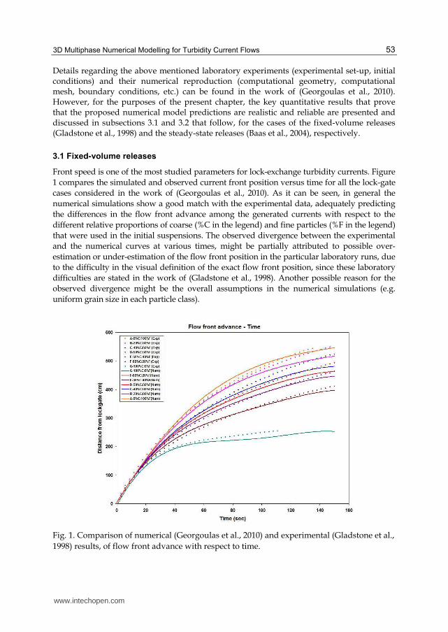
Front speed is one of the most studied parameters for lock-exchange turbidity currents. Figure 1 compares the simulated and observed current front position versus time for all the lock-gate cases considered in the work of (Georgoulas et al., 2010). As it can be seen, in general the numerical simulations show a good match with the experimental data, adequately predicting the differences in the flow front advance among the generated currents with respect to the different relative proportions of coarse (%C in the legend) and fine particles (%F in the legend) that were used in the initial suspensions. The observed divergence between the experimental and the numerical curves at various times, might be partially attributed to possible over-estimation or under-estimation of the flow front position in the particular laboratory runs, due to the difficulty in the visual definition of the exact flow front position, since these laboratory difficulties are stated in the work of (Gladstone et al., 1998). Another possible reason for the observed divergence might be the overall assumptions in the numerical simulations (e.g. uniform grain size in each particle class).

Fig. 1. Comparison of numerical (Georgoulas et al., 2010) and experimental (Gladstone et al., 1998) results, of flow front advance with respect to time.

www.intechopen.com

Numerical Modelling

54

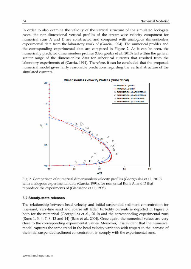
In order to also examine the validity of the vertical structure of the simulated lock-gate cases, the non-dimensional vertical profiles of the stream-wise velocity component for numerical runs A and D are constructed and compared with analogous dimensionless experimental data from the laboratory work of (Garcia, 1994). The numerical profiles and the corresponding experimental data are compared in Figure 2. As it can be seen, the numerically predicted dimensionless profiles (Georgoulas et al., 2010) fall within the general scatter range of the dimensionless data for subcritical currents that resulted from the laboratory experiments of (Garcia, 1994). Therefore, it can be concluded that the proposed numerical model gives fairly reasonable predictions regarding the vertical structure of the simulated currents.

Fig. 2. Comparison of numerical dimensionless velocity profiles (Georgoulas et al., 2010) with analogous experimental data (Garcia, 1994), for numerical Runs A, and D that reproduce the experiments of (Gladstone et al., 1998).

3.2 Steady-state releases

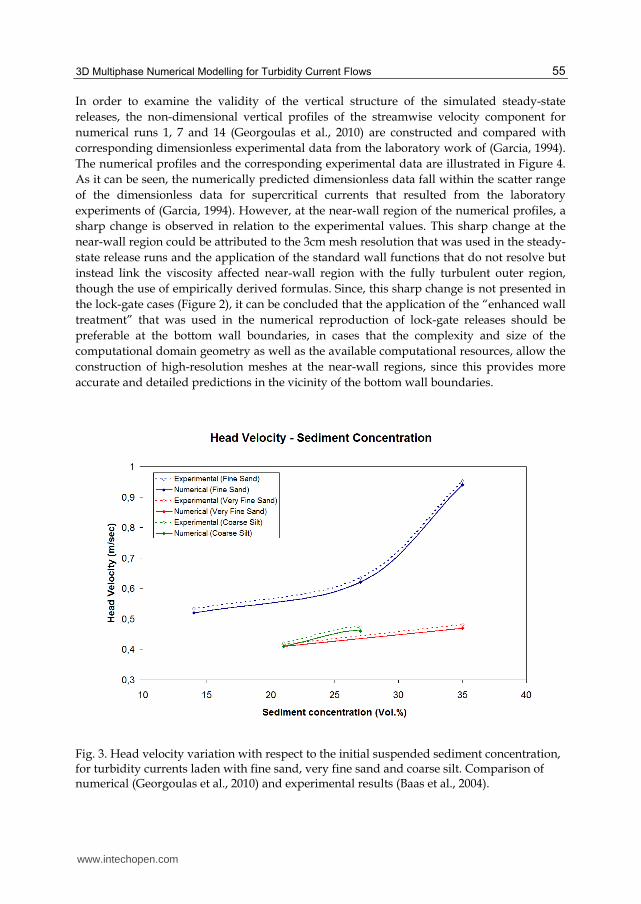
The relationship between head velocity and initial suspended sediment concentration for fine-sand, very-fine sand and coarse silt laden turbidity currents is depicted in Figure 3, both for the numerical (Georgoulas et al., 2010) and the corresponding experimental runs (Runs 1, 3, 4, 7, 8, 13 and 14) (Bass et al., 2004). Once again, the numerical values are very close to the corresponding experimental values. Moreover, it is evident that the numerical model captures the same trend in the head velocity variation with respect to the increase of the initial suspended sediment concentration, in comply with the experimental runs.

www.intechopen.com


55

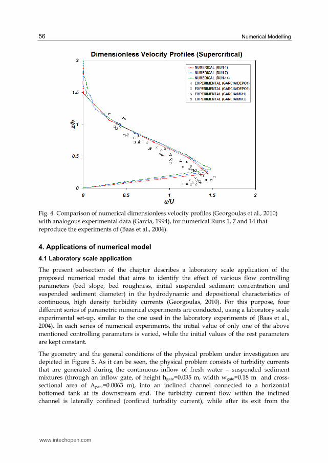
In order to examine the validity of the vertical structure of the simulated steady-state releases, the non-dimensional vertical profiles of the streamwise velocity component for numerical runs 1, 7 and 14 (Georgoulas et al., 2010) are constructed and compared with corresponding dimensionless experimental data from the laboratory work of (Garcia, 1994). The numerical profiles and the corresponding experimental data are illustrated in Figure 4. As it can be seen, the numerically predicted dimensionless data fall within the scatter range of the dimensionless data for supercritical currents that resulted from the laboratory experiments of (Garcia, 1994). However, at the near-wall region of the numerical profiles, a sharp change is observed in relation to the experimental values. This sharp change at the near-wall region could be attributed to the 3cm mesh resolution that was used in the steady-state release runs and the application of the standard wall functions that do not resolve but instead link the viscosity affected near-wall region with the fully turbulent outer region, though the use of empirically derived formulas. Since, this sharp change is not presented in the lock-gate cases (Figure 2), it can be concluded that the application of the “enhanced wall treatment” that was used in the numerical reproduction of lock-gate releases should be preferable at the bottom wall boundaries, in cases that the complexity and size of the computational domain geometry as well as the available computational resources, allow the construction of high-resolution meshes at the near-wall regions, since this provides more accurate and detailed predictions in the vicinity of the bottom wall boundaries.

Fig. 3. Head velocity variation with respect to the initial suspended sediment concentration, for turbidity currents laden with fine sand, very fine sand and coarse silt. Comparison of numerical (Georgoulas et al., 2010) and experimental results (Baas et al., 2004).

www.intechopen.com

Numerical Modelling

56

Fig. 4. Comparison of numerical dimensionless velocity profiles (Georgoulas et al., 2010) with analogous experimental data (Garcia, 1994), for numerical Runs 1, 7 and 14 that reproduce the experiments of (Baas et al., 2004).

4. Applications of numerical model

4.1 Laboratory scale application

The present subsection of the chapter describes a laboratory scale application of the proposed numerical model that aims to identify the effect of various flow controlling parameters (bed slope, bed roughness, initial suspended sediment concentration and suspended sediment diameter) in the hydrodynamic and depositional characteristics of continuous, high density turbidity currents (Georgoulas, 2010). For this purpose, four different series of parametric numerical experiments are conducted, using a laboratory scale experimental set-up, similar to the one used in the laboratory experiments of (Baas et al., 2004). In each series of numerical experiments, the initial value of only one of the above mentioned controlling parameters is varied, while the initial values of the rest parameters are kept constant.

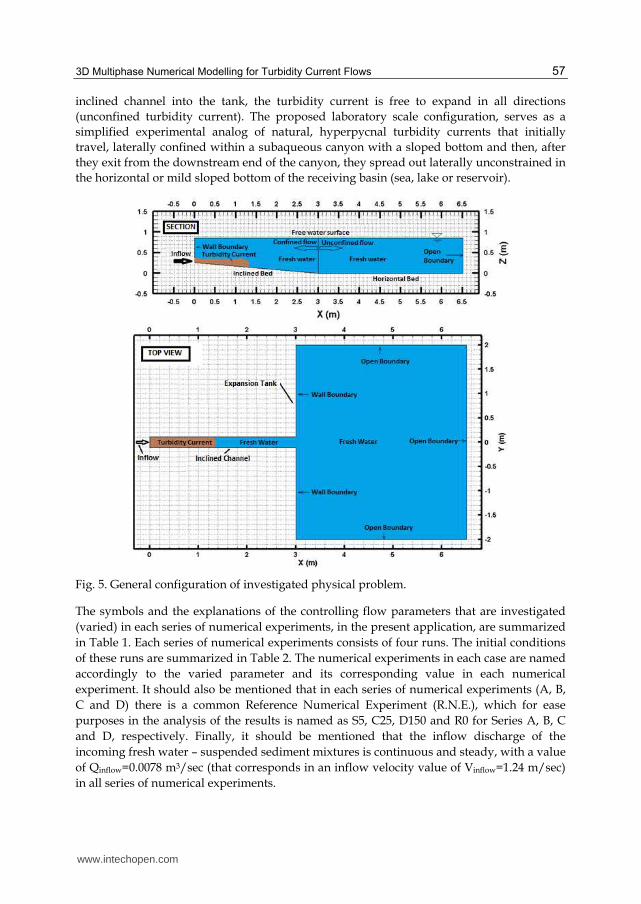
The geometry and the general conditions of the physical problem under investigation are depicted in Figure 5. As it can be seen, the physical problem consists of turbidity currents that are generated during the continuous inflow of fresh water – suspended sediment mixtures (through an inflow gate, of height hgate=0.035 m, width wgate=0.18 m and cross-sectional area of Agate=0.0063 m), into an inclined channel connected to a horizontal bottomed tank at its downstream end. The turbidity current flow within the inclined channel is laterally confined (confined turbidity current), while after its exit from the

www.intechopen.com


57

inclined channel into the tank, the turbidity current is free to expand in all directions (unconfined turbidity current). The proposed laboratory scale configuration, serves as a simplified experimental analog of natural, hyperpycnal turbidity currents that initially travel, laterally confined within a subaqueous canyon with a sloped bottom and then, after they exit from the downstream end of the canyon, they spread out laterally unconstrained in the horizontal or mild sloped bottom of the receiving basin (sea, lake or reservoir).

Fig. 5. General configuration of investigated physical problem.

The symbols and the explanations of the controlling flow parameters that are investigated (varied) in each series of numerical experiments, in the present application, are summarized in Table 1. Each series of numerical experiments consists of four runs. The initial conditions of these runs are summarized in Table 2. The numerical experiments in each case are named accordingly to the varied parameter and its corresponding value in each numerical experiment. It should also be mentioned that in each series of numerical experiments (A, B, C and D) there is a common Reference Numerical Experiment (R.N.E.), which for ease purposes in the analysis of the results is named as S5, C25, D150 and R0 for Series A, B, C and D, respectively. Finally, it should be mentioned that the inflow discharge of the incoming fresh water – suspended sediment mixtures is continuous and steady, with a value of Qinflow=0.0078 m3/sec (that corresponds in an inflow velocity value of Vinflow=1.24 m/sec) in all series of numerical experiments.

www.intechopen.com

Numerical Modelling

58

Series of Numerical

Experiments

Investigated/Varied Parameter

Symbol Explanation

ペ Channel slope Si "inclination angle of channel bed"

ボ Suspended sediment

concentration Ci

"Initial, volumetric concentration of suspended sediment particles in the

inflow mixture"

C Grain diameter Di "Grain diameter of suspended sediment

particles in the inflow mixture"

D Bed roughness Ri

"Roughness of channel and tank bed expressed as equivalent roughness of

uniformly distributed suspended sediment particles of specific grain size"

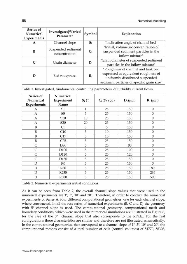
Table 1. Investigated, fundamental controlling parameters, of turbidity current flows.

Series of Numerical

Experiments

Numerical Experiment

Name Si (°) Ci (% vol.) Di (μm) Ri (μm)

A S1 1 25 150 0 A S5 5 25 150 0 A S10 10 25 150 0 A S20 20 25 150 0 B C5 5 5 150 0 B C10 5 10 150 0 B C15 5 15 150 0 B C25 5 25 150 0 C D80 5 25 80 0 C D100 5 25 100 0 C D120 5 25 120 0 C D150 5 25 150 0 D R0 5 25 150 0 D R80 5 25 150 80 D R235 5 25 150 235 D R500 5 25 150 500

Table 2. Numerical experiments initial conditions.

As it can be seen from Table 2, the overall channel slope values that were used in the numerical experiments are 1º, 5º, 10º and 20º. Therefore, in order to conduct the numerical experiments of Series A, four different computational geometries, one for each channel slope, where constructed. In all the rest series of numerical experiments (B, C and D) the geometry with 5º channel slope is used. The computational geometry, computational mesh and boundary conditions, which were used in the numerical simulations are illustrated in Figure 6, for the case of the 5º channel slope that also corresponds to the R.N.E.. For the rest configurations these characteristics are similar and therefore are not illustrated schematically. In the computational geometries, that correspond to a channel slope of 1º, 5º, 10º and 20º, the computational meshes consist of a total number of cells (control volumes) of 51770, 58398,

www.intechopen.com


59

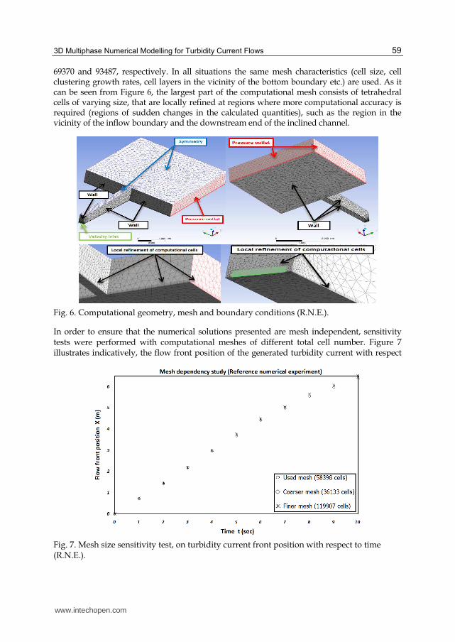
69370 and 93487, respectively. In all situations the same mesh characteristics (cell size, cell clustering growth rates, cell layers in the vicinity of the bottom boundary etc.) are used. As it can be seen from Figure 6, the largest part of the computational mesh consists of tetrahedral cells of varying size, that are locally refined at regions where more computational accuracy is required (regions of sudden changes in the calculated quantities), such as the region in the vicinity of the inflow boundary and the downstream end of the inclined channel.

Fig. 6. Computational geometry, mesh and boundary conditions (R.N.E.).

In order to ensure that the numerical solutions presented are mesh independent, sensitivity tests were performed with computational meshes of different total cell number. Figure 7 illustrates indicatively, the flow front position of the generated turbidity current with respect

Fig. 7. Mesh size sensitivity test, on turbidity current front position with respect to time (R.N.E.).

www.intechopen.com

Numerical Modelling

60

to time, for three different computational meshes in the case of the R.N.E. The first computational mesh is the one used in the simulations (58,398 computational cells), the second one is a coarser mesh (36,133 computational cells) and the third one is a finer mesh (119,907 computational cells). It is obvious (Figure 7) that the resulting curves in each case show a good degree of convergence and therefore the solution can be considered to be mesh independent. In more detail, comparing the results of the coarser mesh with the corresponding results of the finer mesh, it is concluded that increasing the total number of cells by a factor of 3.33, the average differences of the flow front position values with respect to time is only 1.85%.

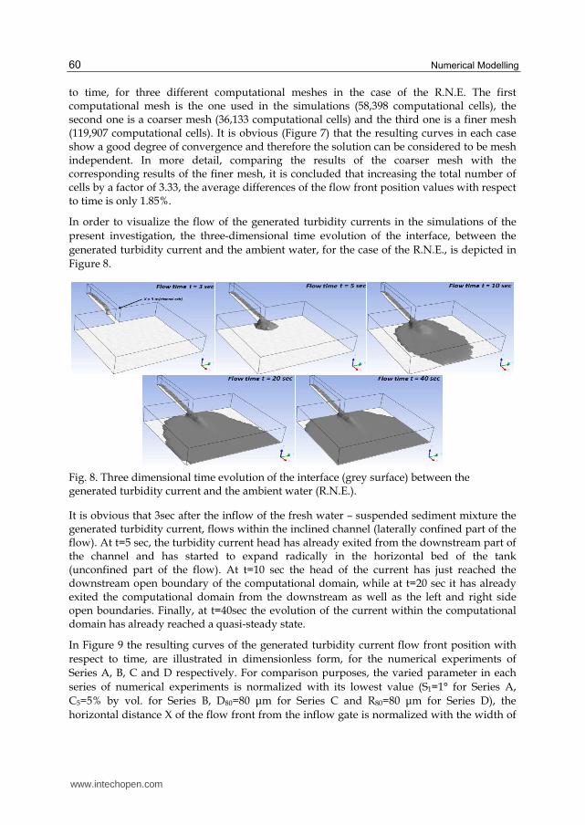
In order to visualize the flow of the generated turbidity currents in the simulations of the present investigation, the three-dimensional time evolution of the interface, between the generated turbidity current and the ambient water, for the case of the R.N.E., is depicted in Figure 8.

Fig. 8. Three dimensional time evolution of the interface (grey surface) between the generated turbidity current and the ambient water (R.N.E.).

It is obvious that 3sec after the inflow of the fresh water – suspended sediment mixture the generated turbidity current, flows within the inclined channel (laterally confined part of the flow). At t=5 sec, the turbidity current head has already exited from the downstream part of the channel and has started to expand radically in the horizontal bed of the tank (unconfined part of the flow). At t=10 sec the head of the current has just reached the downstream open boundary of the computational domain, while at t=20 sec it has already exited the computational domain from the downstream as well as the left and right side open boundaries. Finally, at t=40sec the evolution of the current within the computational domain has already reached a quasi-steady state.

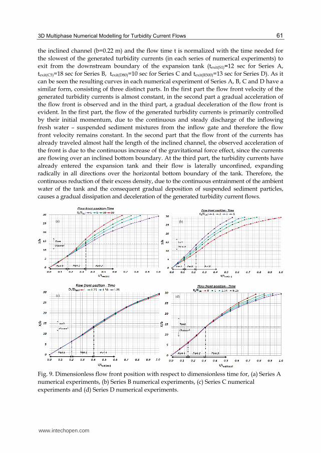
In Figure 9 the resulting curves of the generated turbidity current flow front position with respect to time, are illustrated in dimensionless form, for the numerical experiments of Series A, B, C and D respectively. For comparison purposes, the varied parameter in each series of numerical experiments is normalized with its lowest value (S1=1° for Series A, C5=5% by vol. for Series B, D80=80 ┤m for Series C and R80=80 ┤m for Series D), the horizontal distance X of the flow front from the inflow gate is normalized with the width of

www.intechopen.com


61

the inclined channel (b=0.22 m) and the flow time t is normalized with the time needed for the slowest of the generated turbidity currents (in each series of numerical experiments) to exit from the downstream boundary of the expansion tank (texit(S1)=12 sec for Series A, texit(C5)=18 sec for Series B, texit(D80)=10 sec for Series C and texit(R500)=13 sec for Series D). As it can be seen the resulting curves in each numerical experiment of Series A, B, C and D have a similar form, consisting of three distinct parts. In the first part the flow front velocity of the generated turbidity currents is almost constant, in the second part a gradual acceleration of the flow front is observed and in the third part, a gradual deceleration of the flow front is evident. In the first part, the flow of the generated turbidity currents is primarily controlled by their initial momentum, due to the continuous and steady discharge of the inflowing fresh water – suspended sediment mixtures from the inflow gate and therefore the flow front velocity remains constant. In the second part that the flow front of the currents has already traveled almost half the length of the inclined channel, the observed acceleration of the front is due to the continuous increase of the gravitational force effect, since the currents are flowing over an inclined bottom boundary. At the third part, the turbidity currents have already entered the expansion tank and their flow is laterally unconfined, expanding radically in all directions over the horizontal bottom boundary of the tank. Therefore, the continuous reduction of their excess density, due to the continuous entrainment of the ambient water of the tank and the consequent gradual deposition of suspended sediment particles, causes a gradual dissipation and deceleration of the generated turbidity current flows.

Fig. 9. Dimensionless flow front position with respect to dimensionless time for, (a) Series A numerical experiments, (b) Series B numerical experiments, (c) Series C numerical experiments and (d) Series D numerical experiments.

(a) (b)

(c) (d)

www.intechopen.com

Numerical Modelling

62

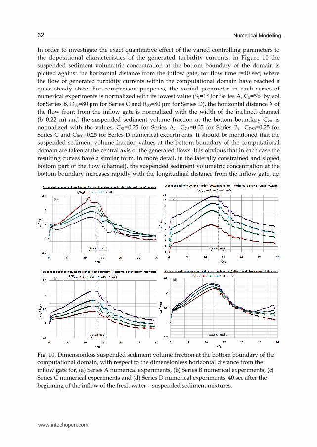
In order to investigate the exact quantitative effect of the varied controlling parameters to the depositional characteristics of the generated turbidity currents, in Figure 10 the suspended sediment volumetric concentration at the bottom boundary of the domain is plotted against the horizontal distance from the inflow gate, for flow time t=40 sec, where the flow of generated turbidity currents within the computational domain have reached a quasi-steady state. For comparison purposes, the varied parameter in each series of numerical experiments is normalized with its lowest value (S1=1° for Series A, C5=5% by vol. for Series B, D80=80 ┤m for Series C and R80=80 ┤m for Series D), the horizontal distance X of the flow front from the inflow gate is normalized with the width of the inclined channel (b=0.22 m) and the suspended sediment volume fraction at the bottom boundary Cvol is normalized with the values, CS1=0.25 for Series A, CC5=0.05 for Series B, CD80=0.25 for Series C and CR80=0.25 for Series D numerical experiments. It should be mentioned that the suspended sediment volume fraction values at the bottom boundary of the computational domain are taken at the central axis of the generated flows. It is obvious that in each case the resulting curves have a similar form. In more detail, in the laterally constrained and sloped bottom part of the flow (channel), the suspended sediment volumetric concentration at the bottom boundary increases rapidly with the longitudinal distance from the inflow gate, up

Fig. 10. Dimensionless suspended sediment volume fraction at the bottom boundary of the computational domain, with respect to the dimensionless horizontal distance from the inflow gate for, (a) Series A numerical experiments, (b) Series B numerical experiments, (c) Series C numerical experiments and (d) Series D numerical experiments, 40 sec after the beginning of the inflow of the fresh water – suspended sediment mixtures.

(a) (b)

(c) (d)

www.intechopen.com


63

to a distance of X/b=1 and then follows a less rapid increase up to a maximum value, at a distance of X/b=11 that is close to the downstream end of the channel (X/b=13.6). The rapid increase of the volume fraction values in the vicinity of the inflow point (X/b=0 to 1) is probably due to the local increase of the volume fraction value of the inflowing mixtures, as a result of the resistance that is exerted from the ambient fluid. In the unconstrained and horizontal bottom part of the flow (tank), the suspended sediment volumetric concentration follows an irregular decrease with respect to the longitudinal distance, reaching an almost constant minimum value in the vicinity of the downstream boundary of the computational domain. The fact that in all cases, the maximum value of the suspended sediment volumetric concentration at the bottom boundary of the computational domain is found near the downstream end of the channel, is probably due to the sudden reduction in the velocity of the generated turbidity currents which is a result of the flow transition from the laterally constrained (channel) to the unconstrained (tank) part of the computational domain. This sudden drop of velocity is reasonable to cause intense particle deposition just upstream of the channel exit to the expansion tank.

Examining separately the effect of each controlling parameter in the flow front advance velocity and in the deposit density of the current at the bottom boundary, it can be concluded that in general, the increase of the channel slope causes an increase in the flow front advance velocity and a reduction in the deposit density. The increase of the initial suspended sediment concentration causes an increase both in the flow front advance velocity and in the deposit density. The increase of the suspended sediment grain diameter causes an increase both in the flow front advance velocity and in the deposit density. Finally, the increase of the bed roughness causes a reduction in the flow front advance velocity and an increase in the deposit density.

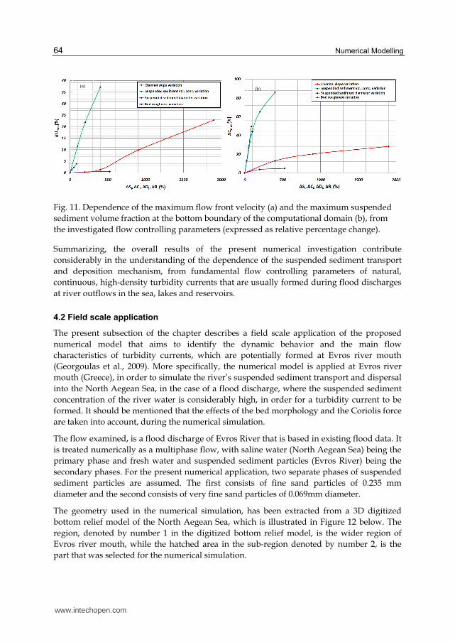
From the presentation and the analysis of the above results so far, it is evident that the investigated controlling parameters affect with a different way and in a comparably different degree the dynamic and depositional characteristics of turbidity currents. Therefore in order to compare the relative percentage effect of the varied controlling parameters in the main flow characteristics of the generated turbidity currents, Figure 11 presents diagrams of the relative percentage change of the maximum flow front advance velocity (Figure 11 a) and the maximum value of suspended sediment volume fraction at the bottom boundary (Figure 11 b), in relation to the relative percentage change of the varied controlling parameters. It should be mentioned that for comparison purposes, the relative percentage change in each case is calculated using absolute differences. It should also be mentioned that in the case of Series D numerical experiments, only the experiments R80, R235, and R500 are taken into consideration, where the values of the bottom boundary roughness are greater than zero. It is obvious that the variation of the initial suspended sediment concentration as well as the suspended sediment grain diameter have the biggest effect in the flow of the generated turbidity currents. This can be probably attributed to the direct effect of the proposed controlling parameters in the main driving force of turbidity currents, which is the excess density of the current in relation to the ambient water density. The variation of the bed roughness has the smallest effect, while the variation of the channel slope causes a moderate effect in the turbidity current flows, in relation to the rest controlling parameters.

www.intechopen.com

Numerical Modelling

64

Fig. 11. Dependence of the maximum flow front velocity (a) and the maximum suspended sediment volume fraction at the bottom boundary of the computational domain (b), from the investigated flow controlling parameters (expressed as relative percentage change).

Summarizing, the overall results of the present numerical investigation contribute considerably in the understanding of the dependence of the suspended sediment transport and deposition mechanism, from fundamental flow controlling parameters of natural, continuous, high-density turbidity currents that are usually formed during flood discharges at river outflows in the sea, lakes and reservoirs.

4.2 Field scale application

The present subsection of the chapter describes a field scale application of the proposed numerical model that aims to identify the dynamic behavior and the main flow characteristics of turbidity currents, which are potentially formed at Evros river mouth (Georgoulas et al., 2009). More specifically, the numerical model is applied at Evros river mouth (Greece), in order to simulate the river’s suspended sediment transport and dispersal into the North Aegean Sea, in the case of a flood discharge, where the suspended sediment concentration of the river water is considerably high, in order for a turbidity current to be formed. It should be mentioned that the effects of the bed morphology and the Coriolis force are taken into account, during the numerical simulation.

The flow examined, is a flood discharge of Evros River that is based in existing flood data. It is treated numerically as a multiphase flow, with saline water (North Aegean Sea) being the primary phase and fresh water and suspended sediment particles (Evros River) being the secondary phases. For the present numerical application, two separate phases of suspended sediment particles are assumed. The first consists of fine sand particles of 0.235 mm diameter and the second consists of very fine sand particles of 0.069mm diameter.

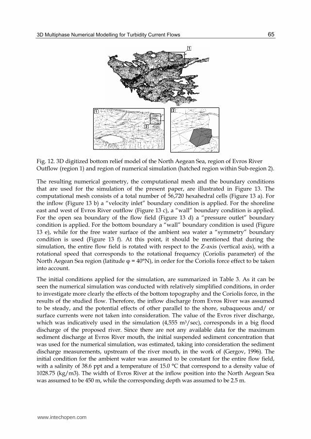
The geometry used in the numerical simulation, has been extracted from a 3D digitized bottom relief model of the North Aegean Sea, which is illustrated in Figure 12 below. The region, denoted by number 1 in the digitized bottom relief model, is the wider region of Evros river mouth, while the hatched area in the sub-region denoted by number 2, is the part that was selected for the numerical simulation.

(a) (b)

www.intechopen.com


65

Fig. 12. 3D digitized bottom relief model of the North Aegean Sea, region of Evros River Outflow (region 1) and region of numerical simulation (hatched region within Sub-region 2).

The resulting numerical geometry, the computational mesh and the boundary conditions that are used for the simulation of the present paper, are illustrated in Figure 13. The computational mesh consists of a total number of 56,720 hexahedral cells (Figure 13 a). For the inflow (Figure 13 b) a “velocity inlet” boundary condition is applied. For the shoreline east and west of Evros River outflow (Figure 13 c), a “wall” boundary condition is applied. For the open sea boundary of the flow field (Figure 13 d) a “pressure outlet” boundary condition is applied. For the bottom boundary a “wall” boundary condition is used (Figure 13 e), while for the free water surface of the ambient sea water a “symmetry” boundary condition is used (Figure 13 f). At this point, it should be mentioned that during the simulation, the entire flow field is rotated with respect to the Z-axis (vertical axis), with a rotational speed that corresponds to the rotational frequency (Coriolis parameter) of the North Aegean Sea region (latitude φ = 40°N), in order for the Coriolis force effect to be taken into account.

The initial conditions applied for the simulation, are summarized in Table 3. As it can be seen the numerical simulation was conducted with relatively simplified conditions, in order to investigate more clearly the effects of the bottom topography and the Coriolis force, in the results of the studied flow. Therefore, the inflow discharge from Evros River was assumed to be steady, and the potential effects of other parallel to the shore, subaqueous and/ or surface currents were not taken into consideration. The value of the Evros river discharge, which was indicatively used in the simulation (4,555 m3/sec), corresponds in a big flood discharge of the proposed river. Since there are not any available data for the maximum sediment discharge at Evros River mouth, the initial suspended sediment concentration that was used for the numerical simulation, was estimated, taking into consideration the sediment discharge measurements, upstream of the river mouth, in the work of (Gergov, 1996). The initial condition for the ambient water was assumed to be constant for the entire flow field, with a salinity of 38.6 ppt and a temperature of 15.0 °C that correspond to a density value of 1028.75 (kg/m3). The width of Evros River at the inflow position into the North Aegean Sea was assumed to be 450 m, while the corresponding depth was assumed to be 2.5 m.

www.intechopen.com

Numerical Modelling

66

Fig. 13. Numerical simulation geometry, computational mesh and boundary conditions.

Inflow discharge (m3/sec) 4,555

Fine sand particle diameter (mm) 0.235

Very fine sand particle diameter (mm) 0.069

Fine sand concentration (vol. %) 0.7%

Very fine sand concentration (vol. %) 0.7%

Saline water density (kg/m3) 1028,75

Fresh water density (kg/m3) 998,2

Sand particle density (kg/m3) 2,650

Coriolis parameter f (Hz) 9.35x10-5

Table 3. Numerical simulation initial conditions.

www.intechopen.com


67

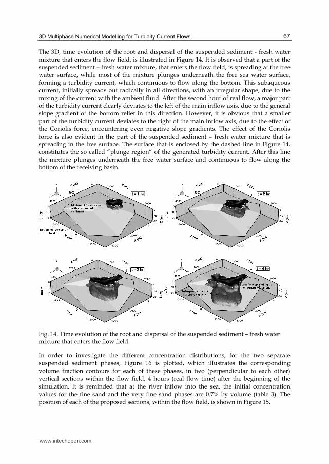
The 3D, time evolution of the root and dispersal of the suspended sediment - fresh water mixture that enters the flow field, is illustrated in Figure 14. It is observed that a part of the suspended sediment – fresh water mixture, that enters the flow field, is spreading at the free water surface, while most of the mixture plunges underneath the free sea water surface, forming a turbidity current, which continuous to flow along the bottom. This subaqueous current, initially spreads out radically in all directions, with an irregular shape, due to the mixing of the current with the ambient fluid. After the second hour of real flow, a major part of the turbidity current clearly deviates to the left of the main inflow axis, due to the general slope gradient of the bottom relief in this direction. However, it is obvious that a smaller part of the turbidity current deviates to the right of the main inflow axis, due to the effect of the Coriolis force, encountering even negative slope gradients. The effect of the Coriolis force is also evident in the part of the suspended sediment – fresh water mixture that is spreading in the free surface. The surface that is enclosed by the dashed line in Figure 14, constitutes the so called “plunge region” of the generated turbidity current. After this line the mixture plunges underneath the free water surface and continuous to flow along the bottom of the receiving basin.

Fig. 14. Time evolution of the root and dispersal of the suspended sediment – fresh water mixture that enters the flow field.

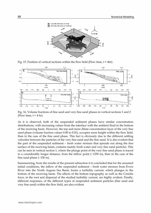
In order to investigate the different concentration distributions, for the two separate suspended sediment phases, Figure 16 is plotted, which illustrates the corresponding volume fraction contours for each of these phases, in two (perpendicular to each other) vertical sections within the flow field, 4 hours (real flow time) after the beginning of the simulation. It is reminded that at the river inflow into the sea, the initial concentration values for the fine sand and the very fine sand phases are 0.7% by volume (table 3). The position of each of the proposed sections, within the flow field, is shown in Figure 15.

www.intechopen.com

Numerical Modelling

68

Fig. 15. Position of vertical sections within the flow field (Flow time, t = 4hr).

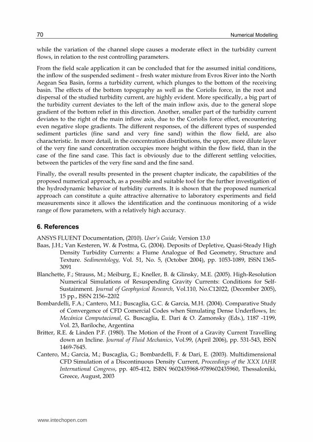
Fig. 16. Volume fractions of fine sand and very fine sand phases in vertical sections 1 and 2 (Flow time, t = 4 hr).

As it is observed, both of the suspended sediment phases have similar concentration distributions, with increasing values from the interface with the ambient fluid to the bottom of the receiving basin. However, the top and more dilute concentration layer of the very fine sand phase (volume fraction values 0.00 to 0.01), occupies more height within the flow field, than in the case of the fine sand phase. This fact is obviously due to the different settling velocities between the particles of the very fine sand and the fine sand. It is also evident that the part of the suspended sediment – fresh water mixture that spreads out along the free surface of the receiving basin, contains mainly fresh water and very fine sand particles. This can be seen in vertical section 1, where the plunge point of the very fine sand phase is traced in a considerably longer distance, from the inflow point (~1250 m), than in the case of the fine sand phase (~150 m).

Summarizing, from the results of the present subsection it is concluded that for the assumed initial conditions, the inflow of the suspended sediment – fresh water mixture from Evros River into the North Aegean Sea Basin, forms a turbidity current, which plunges to the bottom of the receiving basin. The effects of the bottom topography as well as the Coriolis force, in the root and dispersal of the studied turbidity current, are highly evident. Finally, different responses, of the different types of suspended sediment particles (fine sand and very fine sand) within the flow field, are also evident.

www.intechopen.com


69

5. Conclusion

In the present chapter an “uncommon”, CFD-based, three-dimensional, multiphase numerical approach for the simulation and study of the hydrodynamic and depositional characteristics of turbidity currents is presented. The main advantages of the proposed multiphase numerical approach, in relation to previous quasi single-phase approaches are the following:

Separate velocity fields are calculated for each phase (ambient water, inflow/carrier water and various classes of suspended sediment), since the laws for the conservation of mass and momentum are accordingly modified, in order to be satisfied by each phase individually.

The use of the RNG k-ε turbulence model significantly increases the applicability of the proposed numerical approach, as it can also account for turbidity current flows with low Reynolds numbers.

The total number of flow phases that can be simulated is only limited by the available memory of the computational resources. Hence, it can also be used for the simulation of polydisperse turbidity currents that contain many classes of suspended sediment particles, which are more close to natural turbidity current flows.

It can handle a wide range of particulate loading, and therefore is capable for the simulation of both dilute and dense turbidity current flows.

It is based on the finite volume method, and therefore it can be applied in situations with complex geometries, like in the case of turbidity currents that are formed at natural, water basin beds (sea, lakes, reservoirs), where morphological anomalies are usually present.

The method is tested against published laboratory data that are available in the literature and the comparison of the numerical and experimental results indicate that its predictions are realistic and reliable.

The overall results of the laboratory scale application contribute considerably in the understanding of the dependence of the suspended sediment transport and deposition mechanism, from fundamental flow controlling parameters of natural, continuous, high-density turbidity currents that are usually formed during flood discharges at river outflows. It is found that the investigated controlling parameters affect with a different way and in a comparably different degree the dynamic and depositional characteristics of turbidity currents. In more detail, the increase of the channel slope causes an increase in the flow front advance velocity and a reduction in the deposit density. The increase of the initial suspended sediment concentration causes an increase both in the flow front advance velocity and in the deposit density. The increase of the suspended sediment grain diameter causes an increase both in the flow front advance velocity and in the deposit density, while the increase of the bed roughness causes a reduction in the flow front advance velocity and an increase in the deposit density. Finally, from the comparison of the relative percentage effect of each of the examined controlling parameters in the main hydrodynamic and depositional characteristics of the generated turbidity currents, it is found that the variation of the initial suspended sediment concentration as well as the suspended sediment grain diameter have the biggest effect, the variation of the bed roughness has the smallest effect,

www.intechopen.com

Numerical Modelling

70

while the variation of the channel slope causes a moderate effect in the turbidity current flows, in relation to the rest controlling parameters.

From the field scale application it can be concluded that for the assumed initial conditions, the inflow of the suspended sediment – fresh water mixture from Evros River into the North Aegean Sea Basin, forms a turbidity current, which plunges to the bottom of the receiving basin. The effects of the bottom topography as well as the Coriolis force, in the root and dispersal of the studied turbidity current, are highly evident. More specifically, a big part of the turbidity current deviates to the left of the main inflow axis, due to the general slope gradient of the bottom relief in this direction. Another, smaller part of the turbidity current deviates to the right of the main inflow axis, due to the Coriolis force effect, encountering even negative slope gradients. The different responses, of the different types of suspended sediment particles (fine sand and very fine sand) within the flow field, are also characteristic. In more detail, in the concentration distributions, the upper, more dilute layer of the very fine sand concentration occupies more height within the flow field, than in the case of the fine sand case. This fact is obviously due to the different settling velocities, between the particles of the very fine sand and the fine sand.

Finally, the overall results presented in the present chapter indicate, the capabilities of the proposed numerical approach, as a possible and suitable tool for the further investigation of the hydrodynamic behavior of turbidity currents. It is shown that the proposed numerical approach can constitute a quite attractive alternative to laboratory experiments and field measurements since it allows the identification and the continuous monitoring of a wide range of flow parameters, with a relatively high accuracy.

6. References

ANSYS FLUENT Documentation, (2010). User’s Guide, Version 13.0 Baas, J.H.; Van Kesteren, W. & Postma, G, (2004). Deposits of Depletive, Quasi-Steady High

Density Turbidity Currents: a Flume Analogue of Bed Geometry, Structure and Texture. Sedimentology, Vol. 51, No. 5, (October 2004), pp. 1053-1089, ISSN 1365-3091

Blanchette, F.; Strauss, M.; Meiburg, E.; Kneller, B. & Glinsky, M.E. (2005). High-Resolution Numerical Simulations of Resuspending Gravity Currents: Conditions for Self-Sustainment. Journal of Geophysical Research, Vol.110, No.C12022, (December 2005), 15 pp., ISSN 2156–2202

Bombardelli, F.A.; Cantero, M.I.; Buscaglia, G.C. & Garcia, M.H. (2004). Comparative Study of Convergence of CFD Comercial Codes when Simulating Dense Underflows, In: Mecánica Computacional, G. Buscaglia, E. Dari & O. Zamonsky (Eds.), 1187 -1199, Vol. 23, Bariloche, Argentina

Britter, R.E. & Linden P.F. (1980). The Motion of the Front of a Gravity Current Travelling down an Incline. Journal of Fluid Mechanics, Vol.99, (April 2006), pp. 531-543, ISSN 1469-7645.

Cantero, M.; Garcia, M.; Buscaglia, G.; Bombardelli, F. & Dari, E. (2003). Multidimensional CFD Simulation of a Discontinuous Density Current, Proceedings of the XXX IAHR International Congress, pp. 405-412, ISBN 9602435968-9789602435960, Thessaloniki, Greece, August, 2003

www.intechopen.com


71

Cantero, M.I.; Balachandar, S. & Garcia, M.H. (2008a). An Eulerian-Eulerian Model for Gravity Currents Driven by Inertial Paricles. International Journal of Multiphase Flow, Vol.34, No.5, (May 2008), pp. 484-501, ISSN 0301-9322

Cantero, M.I.; Balachandar, S.; Garcia, M.H. & Bock, D. (2008b). Turbulent Structures in Planar Gravity Currents and Their Influence on the Flow Dynamics. Journal of Geophysical Research, Vol.113, No. C08018, (August 2008), 22 pp., ISSN 2156–2202

Cebeci, T. & Bradshaw, P. (1977). Momentum transfer in boundary layers. Hemisphere Publishing Corporation, New York.

Farrell, G.J. & Stefan, H.G. (1986). Buoyancy induced plunging flows into reservoirs and coastal regions. Tech.Rep. No.241, At. Anthony Falls Hydr. Lab., Univ. of Minnesota, Minneapolis

Garcia, M. & Parker, G. (1989). Experiments on Hydraulic Jumps in Turbidity Currents near a Canyon-Fan Transition. Science, Vol.245, No.4916, (July 1989), ISSN 1095-9203

Garcia, M. (1994). Depositional Turbidity Currents Laden with Poorly Sorted Sediment. Journal of Hydraulic Engineering, Vol.120, No.11, (November 1994): pp. 1240-1263, ISSN 1943-7900

Georgoulas, A.; Tzanakis, T.; Angelidis, P.; Panagiotidis, T. & Kotsovinos, N. (2009) Numerical Simulation of Suspended Sediment Transport and Dispersal from Evros River into the North Aegean Sea, by the Mechanism of Turbidity Currents, Proceedings of the 11th International Conference on Environmental Science and Technology, Vol. A, pp. 343-350, Chania, Crete, Greece, September 3-5, 2009.

Georgoulas, A.; Panagiotidis, T.; Angelidis, P. & Kotsovinos, N. (2010). 3D Numerical Modelling of Turbidity Currents. Environmental Fluid Mechanics, Vol. 10, No.6, (August 2010), pp. 603-635, ISSN 1573-1510

Georgoulas, A. (2010). Study of the density currents at river outflows, due to suspened sediment particles. PhD Thesis, Democritus University of Thrace (November 2010), Department of Civil Engineering, Xanthi, Greece. Available online:

http://thesis.ekt.gr/thesisBookReader/id/23438#page/8/mode/2up Gergov, G. (1996). Suspended sediment load of Bulgarian rivers. GeoJournal, Vol.40, No.4,

(December 1996), pp. 387-396, ISSN 1572-9893 Gladstone, C.; Phillips, J.C. & Sparks, R.S.J. (1998). Experiments on Bidisperse, Constant-

Volume Gravity Currents: Propagation and Sediment Deposition. Sedimentology, Vol.45, No.5, (October 1998), pp. 833-843, ISSN 1365-3091

Hartel, C.; Meiburg, E. & Necker, F. (2000). Analysis and Direct Numerical Simulation of the Flow at a Gravity-Current Head: Part 1. Flow Topology and Front Speed for Slip and No-Slip Boundaries. Journal of Fluid Mechanics, Vol.418, (September 2000), pp. 189–212, ISSN 1469-7645

Heimsund, S.; Hansen, E.W.M. & Nemec, W. (2002). Computational 3D Fluid-Dynamics Model for Sediment Transport, Erosion and Deposition by Turbidity Currents, In: Abstracts, International Association of Sedimentologists, M. Knoper & B. Cairncross, (Ed.), 151-152, 16th International Sedimentological Congress, Rand Afrikaans Univ., Johannesburg

Huang, H.; Imran, J. & Pirmez, C. (2005). Numerical Model of Turbidity Currents with a Deforming Bottom Boundary. Journal of Hydraulic Engineering, Vol.131, No.4, (April 2005), pp. 283-293, ISSN 0733-9429

www.intechopen.com

Numerical Modelling

72

Imran, J.; Kassem, A. & Khan, S.M. (2004). Three-Dimensional Modelling of Density Current. I. Flow in Straight Confined and Unconfined Channels. Journal of Hydraulic Research, Vol.42, No.6, (August 2010), pp. 578–590, ISSN 1814-2079

Janbu, N. E.; Nemec, W.; Kirman, E. & Özaksoy, V. (2009) Facies Anatomy of a Sand-Rich Channelized Turbiditic System: The Eocene Kusuri Formation in the Sinop Basin, North-Central Turkey, In: Sedimentary Processes, Environments and Basins: A Tribute to Peter Friend, G. Nichols, E. Williams & C. Paola (Eds.), 457-517, Blackwell Publishing Ltd., ISBN 9781405179225, Oxford, UK

Kassem, A. & Imran, J. (2001). Simulation of Turbid Underflows Generated by the Plunging of a River. Geology, Vol.29, No.7, (July 2001), pp.655–658, ISSN 1943-2682

Kneller, B.C.; Bennett, S.J. & McCaffrey, W.D. (1997). Velocity and Turbulence Structure of Density Currents and Internal Solitary Waves: Potential Sediment Transport and the Formation of Wave Ripples in Deep Water. Sedimentary Geology, Vol.112, No.3-4, (September 1997), pp. 235-250, ISSN 0037-0738

Lavelli, A.; Boillat, J.L. & De Cesare, G. (2002). Numerical 3D Modelling of the Vertical Mass Exchange Induced by Turbidity Currents in Lake Lugano (Switzerland), Proceedings of 5th International Conference on Hydro-Science and Engineering (ICHE-2002), Reference: LCH-CONF-2002-012 Note: [355]

Lovell, J.P.B. (1971). Control of Slope on Deposition from Small-Scale Turbidity Currents: Experimental Results and Possible Geological Significance. Sedimentology, Vol.17, No.1-2, (June 2006) pp. 81-88, ISSN 1365-3091

Mehdizadeh, A.; Firoozabadi, B. & Farhanieh, B. (2008). Numerical Simulation of Turbidity

Current Using 2v f Turbulence Model. Journal of Applied Fluid Mechanics, Vol.1,

No. 2, pp. 45-55, ISSN 1735-3645 Mulder, T. & Alexander, J. (2001). The Physical Character of Subaqueous Sedimentary

Density Flows and their Deposits. Sedimentology, Vol.48, No.2, (December 2001), pp. 269-299, ISSN 1365-3091

Necker, F.; Hartel, C.; Kleiser, L. & Meinburg, E. (2002). High-Resolution Simulations of Particle Driven Gravity Currents. International Journal of Multiphase Flow, Vol.28, No.2, (February 2002), pp. 279-300, ISSN: 0301-9322

Ooi, S.K.; Constantinescu, G. & Weber, L.J. (2007). 2D Large-Eddy Simulation of Lock-Exchange Gravity Current Flows at High Grashof Numbers. Journal of Hydraulic Engineering, Vol.133, No.9, (September 2007), pp. 1037-1047, ISSN 0733-9429

Posamentier, H.W. & Kolla, V. (2003). Seismic Geomorphology and Stratigraphy of Depositional Elements in Deep-Water Settings. Journal of Sedimentary Research, Vol.73, No.3, (May 2003), pp. 367-388, ISSN 1527-1404

Saller, A.; Werner, K.; Sugiaman, F.; Cebastiant, A.; May, R.; Glenn, D. & Barker, C. (2008). Characteristics of Pleistocene Deep-Water Fan Lobes and their Application to an Upper Miocene Reservoir Model, Offshore East Kalimantan, Indonesia. AAPG Bulletin, Vol.92, No.7, (July 2008), pp. 919-949, ISSN 0149-1423

Simpson, J.E. & Britter, R.E. (1979). The Dynamics of the Head of a Gravity Current Advancing over a Horizontal Surface. Journal of Fluid Mechanics, Vol. 94, No.3, (April 2006), pp. 477-495, ISSN 1469-7645

Singh, J. (2008). Simulation of Suspension Gravity Currents with Different Initial Aspect Ratio and Layout of Turbidity Fence. Applied Mathematical Modelling, Vol.32, No.11, (November 2008), pp. 2329–2346, ISSN 0307-904X

www.intechopen.com

Numerical ModellingEdited by Dr. Peep Miidla

ISBN 978-953-51-0219-9Hard cover, 398 pagesPublisher InTechPublished online 23, March, 2012Published in print edition March, 2012

InTech EuropeUniversity Campus STeP Ri Slavka Krautzeka 83/A 51000 Rijeka, Croatia Phone: +385 (51) 770 447 Fax: +385 (51) 686 166www.intechopen.com

InTech ChinaUnit 405, Office Block, Hotel Equatorial Shanghai No.65, Yan An Road (West), Shanghai, 200040, China

Phone: +86-21-62489820 Fax: +86-21-62489821

This book demonstrates applications and case studies performed by experts for professionals and students inthe field of technology, engineering, materials, decision making management and other industries in whichmathematical modelling plays a role. Each chapter discusses an example and these are ranging from well-known standards to novelty applications. Models are developed and analysed in details, authors carefullyconsider the procedure for constructing a mathematical replacement of phenomenon under consideration. Formost of the cases this leads to the partial differential equations, for the solution of which numerical methodsare necessary to use. The term Model is mainly understood as an ensemble of equations which describe thevariables and interrelations of a physical system or process. Developments in computer technology andrelated software have provided numerous tools of increasing power for specialists in mathematical modelling.One finds a variety of these used to obtain the numerical results of the book.

How to referenceIn order to correctly reference this scholarly work, feel free to copy and paste the following:

A. Georgoulas, P. Angelidis, K. Kopasakis and N. Kotsovinos (2012). 3D Multiphase Numerical Modelling forTurbidity Current Flows, Numerical Modelling, Dr. Peep Miidla (Ed.), ISBN: 978-953-51-0219-9, InTech,Available from: http://www.intechopen.com/books/numerical-modelling/3d-multiphase-numerical-modelling-for-turbidity-current-flows

3d multiphase numerical modelling for turbidity current flows

Documents