Prof. Ville VuorinenMarch 30th 2020

Aalto University, School of Engineering

AAE-E3030 Numerical Modeling of Multiphase Flows

Lecture 6: Governing equations: Bunsen flame

ILO1: Premixed and non-premixed combustion: The student understands what is premixed combustion and can analyse Bunsen flame development using a provided Matlab code

Relevance: HW3

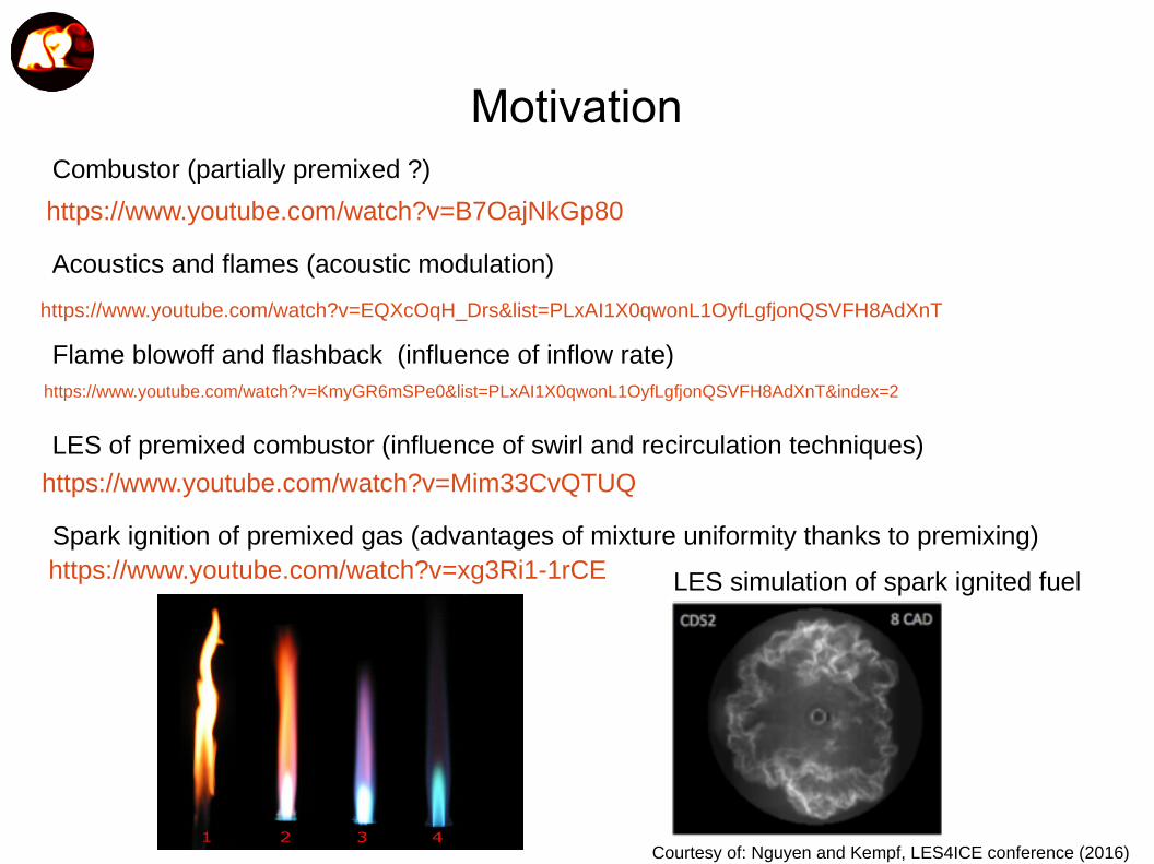
Motivation

https://www.youtube.com/watch?v=B7OajNkGp80

Combustor (partially premixed ?)

https://www.youtube.com/watch?v=Mim33CvQTUQ

Acoustics and flames (acoustic modulation)

Flame blowoff and flashback (influence of inflow rate)

LES of premixed combustor (influence of swirl and recirculation techniques)

https://www.youtube.com/watch?v=xg3Ri1-1rCESpark ignition of premixed gas (advantages of mixture uniformity thanks to premixing)

LES simulation of spark ignited fuel

https://www.youtube.com/watch?v=EQXcOqH_Drs&list=PLxAI1X0qwonL1OyfLgfjonQSVFH8AdXnT

https://www.youtube.com/watch?v=KmyGR6mSPe0&list=PLxAI1X0qwonL1OyfLgfjonQSVFH8AdXnT&index=2

Courtesy of: Nguyen and Kempf, LES4ICE conference (2016)

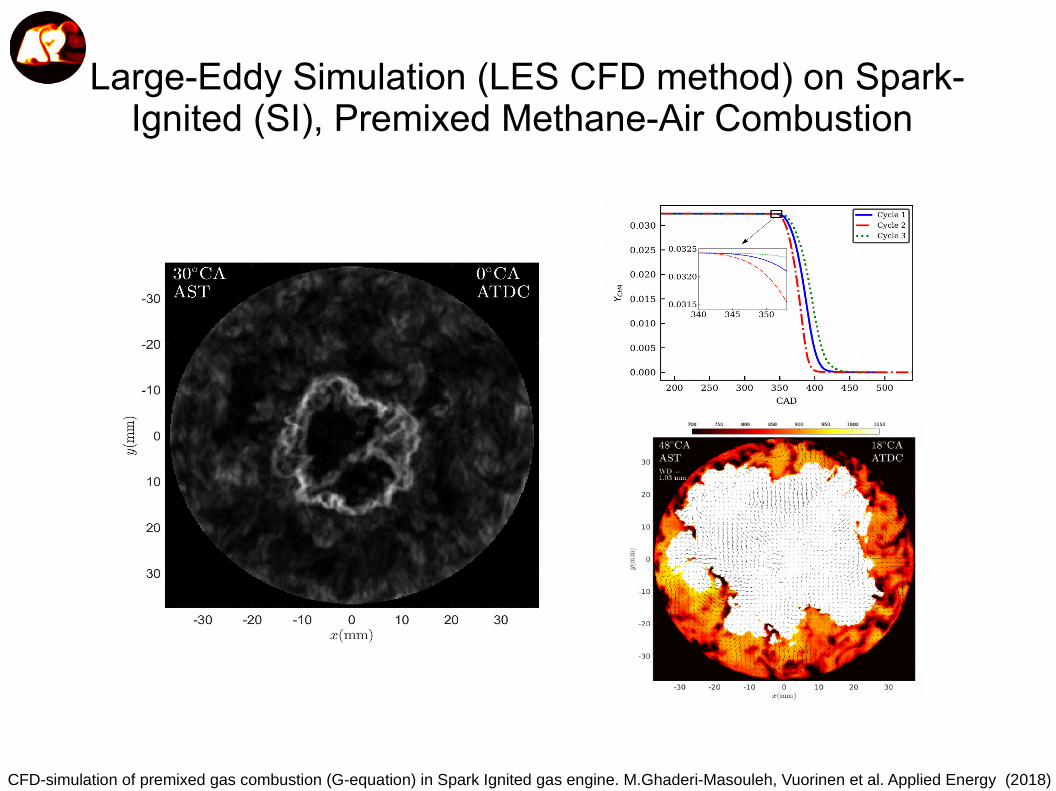
Large-Eddy Simulation (LES CFD method) on Spark-Ignited (SI), Premixed Methane-Air Combustion

CFD-simulation of premixed gas combustion (G-equation) in Spark Ignited gas engine. M.Ghaderi-Masouleh, Vuorinen et al. Applied Energy (2018)

Typical scalar (e.g. concentration of incoming gas A) and velocity fields in a turbulent jet

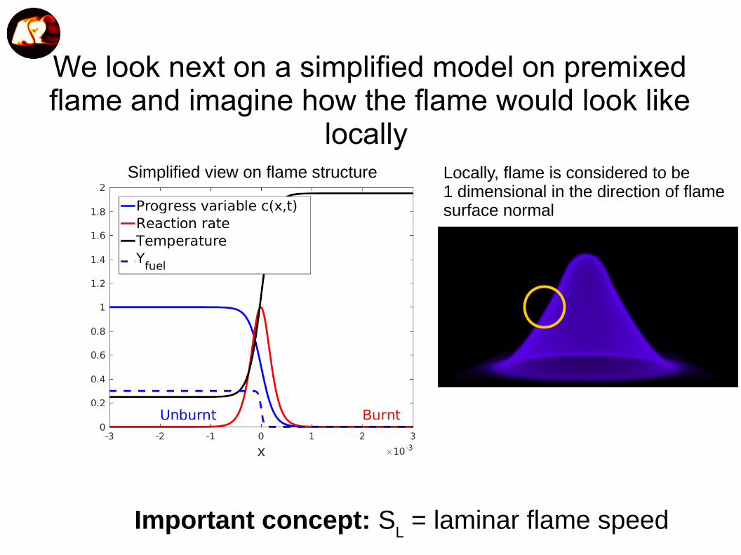
We look next on a simplified model on premixed flame and imagine how the flame would look like

locally Locally, flame is considered to be 1 dimensional in the direction of flame surface normal

Simplified view on flame structure

Important concept: SL = laminar flame speed

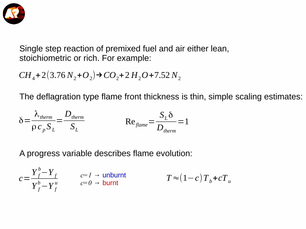
CH 4+2(3.76N2+O2)→CO2+2H2O+7.52N2

Single step reaction of premixed fuel and air either lean, stoichiometric or rich. For example:

The deflagration type flame front thickness is thin, simple scaling estimates:

δ=λ thermρ c pS L

=Dtherm

SLRe flame=

SLδ

Dtherm

=1

A progress variable describes flame evolution:

c=Y fb−Y f

Y fb−Y f

uc=1 → unburntc=0 → burnt

T≈(1−c)T b+cT u

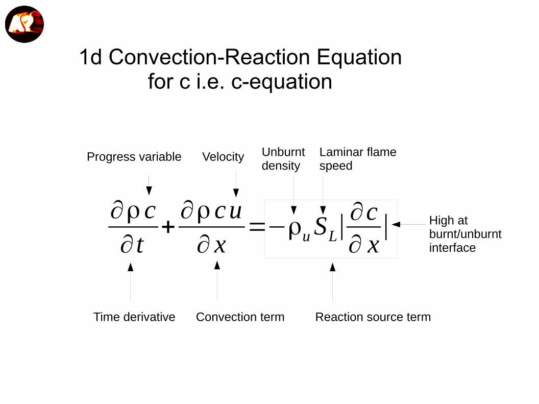
1d Convection-Reaction Equationfor c i.e. c-equation

∂ρ c∂ t

+∂ρ cu∂ x

=−ρuSL|∂c∂ x

|

Time derivative Convection term Reaction source term

Unburnt density

Laminar flamespeed

Progress variable

High at burnt/unburntinterface

Velocity

Progress variable approach in general (1D, 2D and 3D)

∂ρ c∂ t

+∇⋅ρc u=−Sdρu|∇ c|

Sd=displacement speed

Sd=SL (1−LM κ−S)

Markstein length Curvature Strain

Correction terms for curvedand strained plane fronts (deviation from plane flame,uniform ambient flow Assumption).

Correction terms for curvedand strained plane fronts (deviation from plane flame,uniform ambient flow Assumption).

Interplay of thermal diffusion and global reactionrate consumes fuel

κ=∇⋅n

n=∇ c

|∇ c |

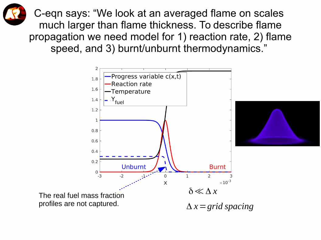
δ≪Δ x

Δ x=grid spacing

C-eqn says: “We look at an averaged flame on scales much larger than flame thickness. To describe flame

propagation we need model for 1) reaction rate, 2) flame speed, and 3) burnt/unburnt thermodynamics.”

The real fuel mass fraction profiles are not captured.

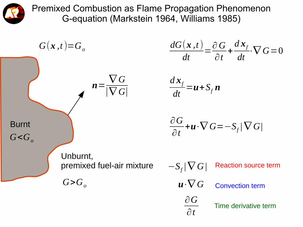
Premixed Combustion as Flame Propagation PhenomenonG-equation (Markstein 1964, Williams 1985)

n=∇G

|∇G|

Burnt

Unburnt, premixed fuel-air mixture

G(x ,t )=Go

G<G o

G>G o

Premixed Combustion as Flame Propagation PhenomenonG-equation (Markstein 1964, Williams 1985)

n=∇G

|∇G|

Burnt

Unburnt, premixed fuel-air mixture

G(x ,t )=Go

G<G o

G>G o

dG(x ,t )dt

=∂G∂ t

+d x fdt

⋅∇G=0

d x fdt

=u+S f n

∂G∂ t

+u⋅∇G=−S f |∇G |

−S f |∇G |

u⋅∇G

∂G∂ t

Reaction source term

Convection term

Time derivative term

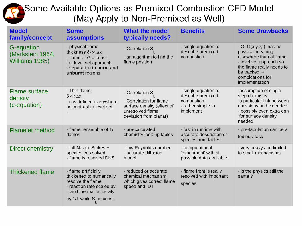
Model family/concept

Some assumptions

What the modeltypically needs?

Benefits Some Drawbacks

G-equation(Markstein 1964,Williams 1985)

- physical flame thickness x - flame at G = const.i.e. level-set approach- separation to burnt and unburnt regions

- Correlation SL

- an algorithm to find the flame position

- single equation to describe premixed combustion

- G=G(x,y,z,t) has no physical meaning elsewhere than at flame- level set approach so the flame really needs to be tracked → compications for implementation

Flame surface density (c-equation)

- Thin flamex - c is defined everywhere in contrast to level-set-

- Correlation SL

- Correlation for flame surface density (effect of unresolved flame deviation from planar)

- single equation to describe premixed combustion- rather simple to implement

-assumption of single step chemistry-a particular link between emissions and c needed- possibly even extra eqn for surface density needed

Flamelet method - flame=ensemble of 1d flames

- pre-calculated chemistry look-up tables

- fast in runtime with accurate description of species from tables

- pre-tabulation can be a

tedious task

Direct chemistry - full Navier-Stokes + species eqs solved- flame is resolved DNS

- low Reynolds number- accurate diffusion model

- computational 'experiment' with all possible data available

- very heavy and limited to small mechanisms

Thickened flame - flame artificially thickened to numerically resolve the flame - reaction rate scaled by L and thermal diffusivity

by 1/L while SL is const.

- reduced or accurate chemical mechanism which gives correct flame speed and IDT

- flame front is really resolved with important

species

- is the physics still the same ?

Some Available Options as Premixed Combustion CFD Model (May Apply to Non-Premixed as Well)

Bunsen Flame – BackgroundρU sin (α)=ρuSL

Assumptions of this eqn?

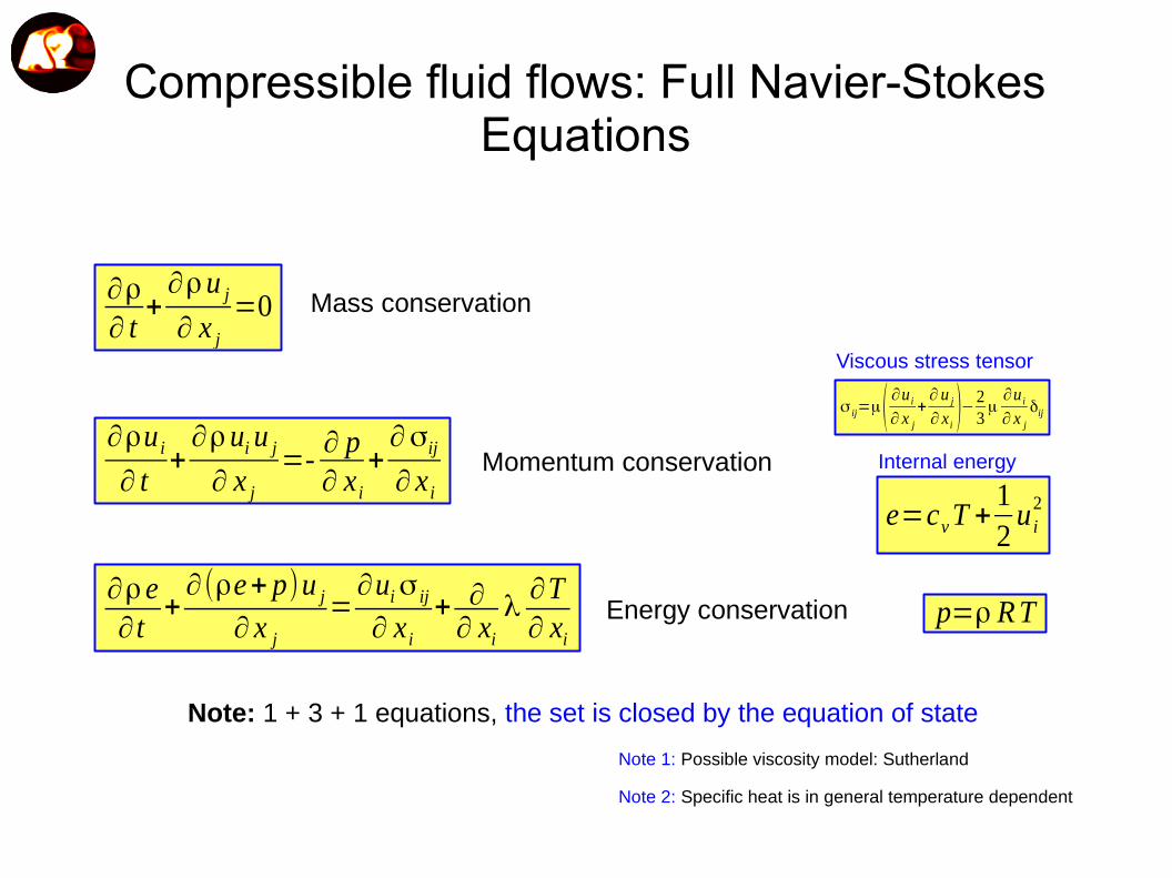
Compressible fluid flows: Full Navier-Stokes Equations

∂ρ∂ t

+∂ρu j∂ x j

=0

∂ρu i∂ t

+∂ρuiu j∂ x j

=-∂ p∂ x i

+∂σij∂ x i

∂ρ e∂ t

+∂(ρe+ p)u j

∂ x j=

∂uiσ ij

∂ x i+ ∂

∂ xiλ

∂T∂ xi

Mass conservation

Momentum conservation

Energy conservation

σ ij=μ ( ∂u i∂ x j

+∂ u j∂ x i )−

23μ

∂u i∂ x j

δij

Viscous stress tensor

e=cvT +12u i

2

p=ρ RT

Internal energy

Note 1: Possible viscosity model: Sutherland

Note 2: Specific heat is in general temperature dependent

Note: 1 + 3 + 1 equations, the set is closed by the equation of state

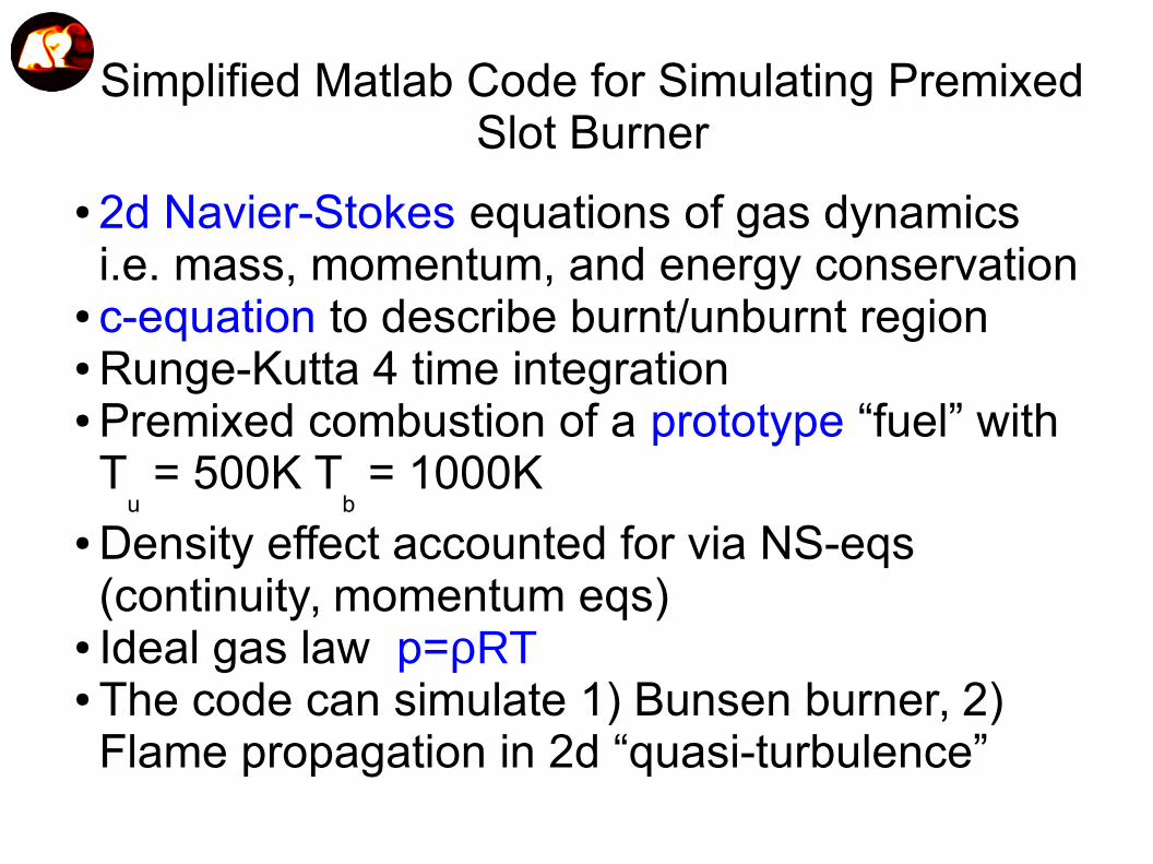
Simplified Matlab Code for Simulating Premixed Slot Burner

● 2d Navier-Stokes equations of gas dynamicsi.e. mass, momentum, and energy conservation

● c-equation to describe burnt/unburnt region● Runge-Kutta 4 time integration● Premixed combustion of a prototype “fuel” with T

u = 500K T

b = 1000K

● Density effect accounted for via NS-eqs (continuity, momentum eqs)

● Ideal gas law p=ρRT● The code can simulate 1) Bunsen burner, 2) Flame propagation in 2d “quasi-turbulence”

Bunsen Flame – Domain Modeled as a 2d “Slot” Burner in the Matlab Code

WallsBC:- U,V → no-slip- p and T → zero gradient- c →zero gradient

Walls

Governing eqs- Compressible Navier-Stokes- Density based approach → p=ρRT- 2nd order space, 4th order time- Progress variable equation (S

L and curvature)

- explicit filtering to stabilize numerically- Temperature source to link c with T

u and T

b

- Tu = 500K T

b = 1000K

- Density variations accounted naturally via continuity eqn and equation of state

Inlet-parabolicvelocity (V

max=

100m/s)-T=Tu- p → zerogradient

Outlet - simple zero gradient for all flow quantities

Computationaldomain

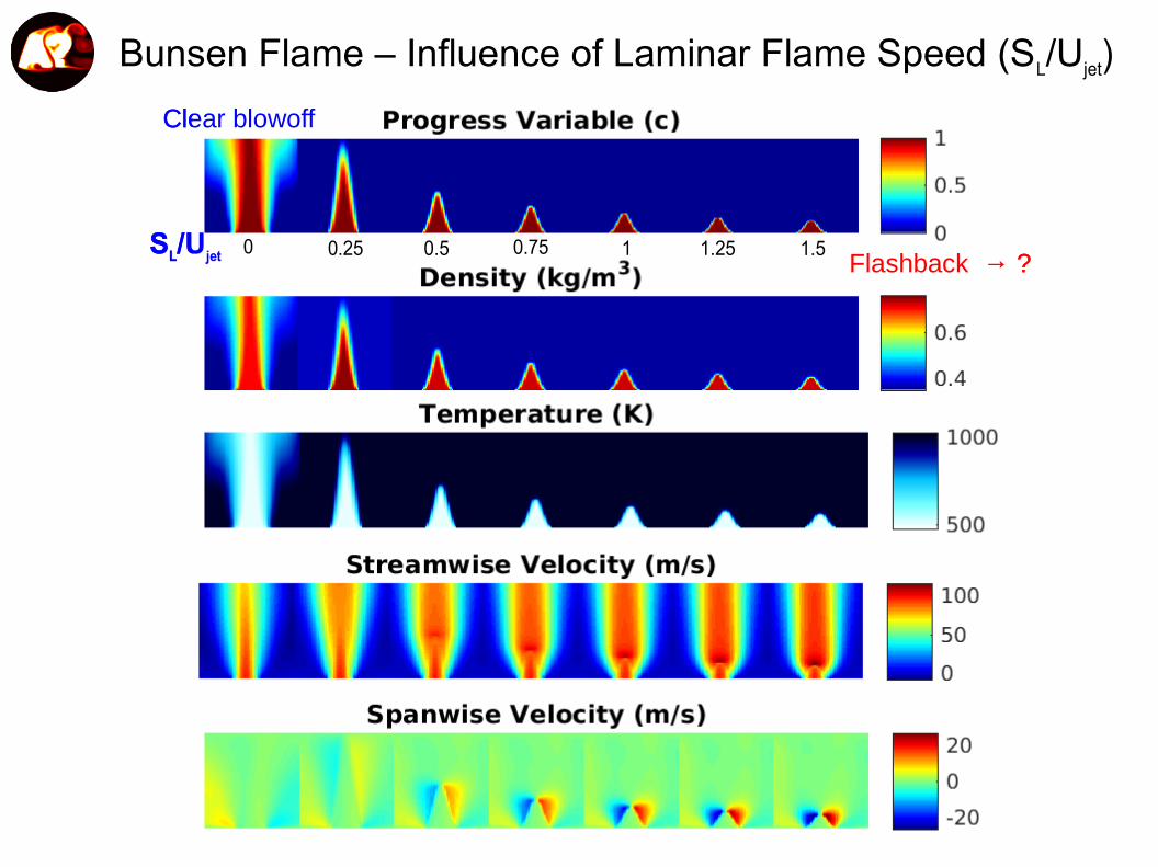
SL/Ujet 0 0.25 0.5 0.75 1 1.25 1.5Flashback → ?

Clear blowoff

SL/Ujet 0 0.25 0.5 0.75 1 1.25 1.5Flashback → ?

Clear blowoff

Bunsen Flame – Influence of Laminar Flame Speed (SL/Ujet)

Bunsen Flame – Burnt vs Unburnt Density

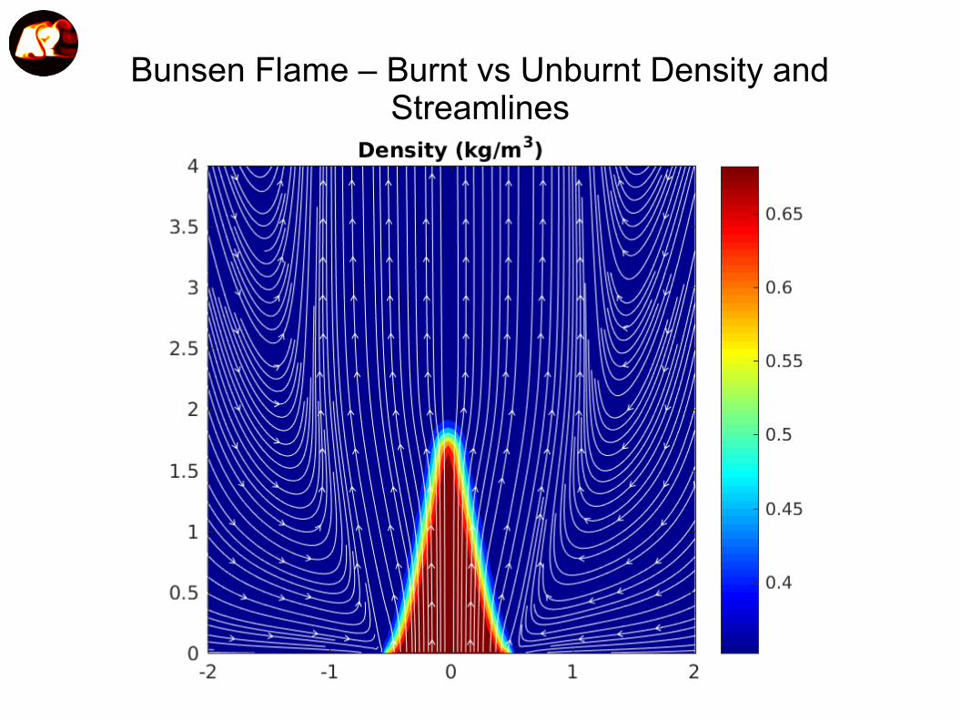
Bunsen Flame – Burnt vs Unburnt Density and Streamlines

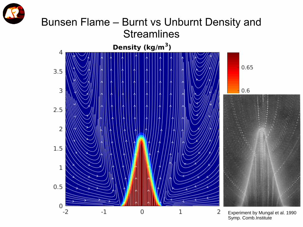
Bunsen Flame – Burnt vs Unburnt Density and Streamlines

Experiment by Mungal et al. 1990Symp. Comb.Institute

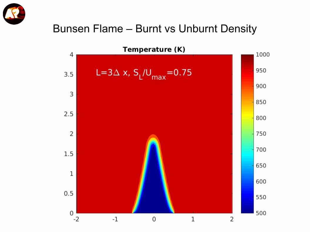
Bunsen Flame – Burnt vs Unburnt Density

Progress variable source term (combustion happens)

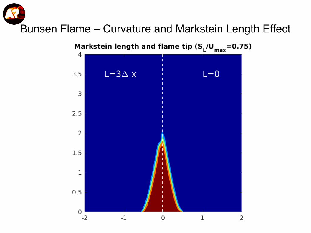
Bunsen Flame – Curvature and Markstein Length Effect

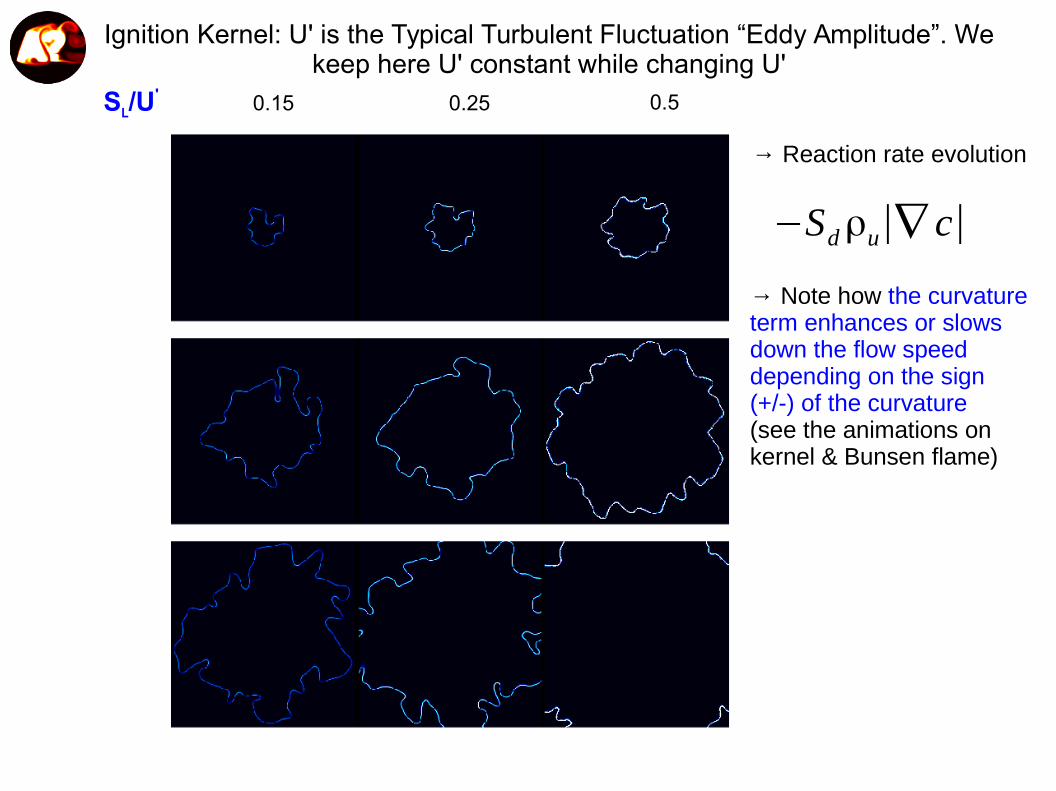
SL/U' 0.15 0.50.25

→ Reaction rate evolution

−Sdρu|∇ c|

→ Note how the curvatureterm enhances or slowsdown the flow speed depending on the sign (+/-) of the curvature (see the animations on kernel & Bunsen flame)

Ignition Kernel: U' is the Typical Turbulent Fluctuation “Eddy Amplitude”. We keep here U' constant while changing U'

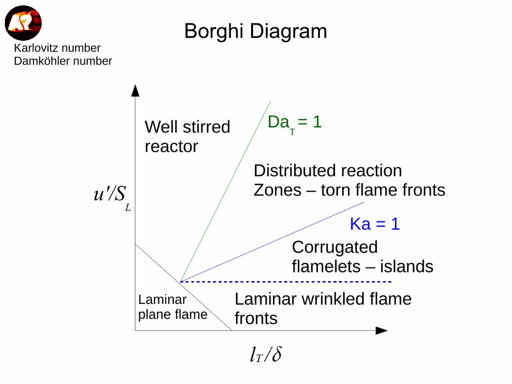
Karlovitz numberDamköhler number

Borghi Diagram