1

Multichannel inversion of scattered teleseismic body waves:

practical considerations and applicability

S. Rondenay,1, M.G. Bostock,2, and K.M. Fischer,1

Short title: MULTICHANNEL SCATTERED WAVE INVERSION

2

Abstract. We investigate the resolving power and applicability of a recently

developed technique for multichannel inversion of scattered teleseismic body waves

recorded at dense seismic arrays. The problem is posed for forward- and back-scattered

wavefields generated at discontinuities in a 2D isotropic medium, with the backprojection

operator cast as a generalized Radon transform (GRT). The approach allows for the

treatment of incident planar waves from arbitrary backazimuths, and recovers estimates

of material property perturbations about a smoothly varying reference model. An

investigation of the main factors affecting resolution indicates that: (1) comprehensive

source/station coverage is necessary to optimize geometrical resolution and recover

accurate material property perturbations; (2) the range in dip resolution diminishes with

increasing depth and is inversely proportional to array width (e.g., reaches [-45◦,45◦]

at depths equivalent to ∼1/2 array width); (3) distortion of the image due to spatial

aliasing is only significant at depths ≤2×[station spacing]; and (4) unaccounted for

departures from model assumptions (smooth variations, isotropy, and 2D geometry)

result in defocusing and mismapping of structure. Two applications to field data

are presented. The first considers data from the Abitibi 1996 broadband array, in

which stations were deployed at ∼20 km intervals. Results show that this level of

spatial sampling, which is characteristic of common broadband arrays, is sufficient to

adequately resolve structure at depths greater than mid-crustal levels. The second

application involves short period data from the Los Angeles Region Seismic Experiment

and shows that images obtained from high frequency records are subject to significant

contamination by scattered surface waves.

3

1. Introduction

One of the current challenges faced by earthquake seismologists is the development of

new tools for high-resolution imaging of the lithosphere and underlying mantle. While

tomographic methods using transmitted body waves [Aki et al., 1977; VanDecar, 1991;

Grand, 1994; van der Hilst et al., 1997] and surface waves [van der Lee and Nolet,

1997; Li et al., 2002] have proven to be powerful tools for volumetric imaging of seismic

anomalies, a wealth of complementary information on the bounding discontinuity of

these anomalies can be obtained from secondary scattered waves in the coda of body

waves. The relative arrival time and amplitude of these secondary waves are indicative

of the position and magnitude of discontinuities in elastic parameters of the subsurface.

The teleseismic P wavefield is of particular interest as it benefits from generally higher

signal-to-noise ratio than other (later arriving) primary phases. Scattered waves, notably

P-to-S conversions, recorded at single stations have thus been utilized for over two

decades as a basis for 1-D modelling of planar discontinuities in the lithosphere [Vinnik,

1977; Langston, 1979]. In recent years, a substantial increase in availability and fidelity

of recording instruments has led to new opportunities for multichannel processing of

scattered teleseismic bodywaves, allowing for 2D/3D imaging of subsurface structure.

Many of these approaches are similar to industry-oriented (e.g., migration) techniques

and generate analogous high resolution depth sections of the subsurface, down to the

mantle transition zone.

Recently developed methods form a continuum with respect to the level of

complexity adopted in the treatment of the scattering problem. On one end of the

spectrum, images may be produced by simple stacking of normalized P-to-S conversion

records (i.e., receiver functions - RF), which are binned according to common conversion

points (CCP) and mapped to depth [Dueker and Sheehan, 1997]. Finer resolution can be

achieved through the stacking of singly scattered wavefields along diffraction hyperbolae

to recover relative scattering intensity/potential at individual points through a 2D or 3D

4

model space [Revenaugh, 1995a; Ryberg and Weber, 2000; Sheehan et al., 2000]. Moving

to higher levels of complexity, methods involving inversion/backprojection operators

[Bostock and Rondenay, 1999; Bostock et al., 2001] and full 3D waveform inversion

[Frederiksen and Revenaugh, 2002] of scattered teleseismic body waves recover estimates

of localized material property perturbations with respect to an a priori background

model.

In this paper, we explore the domains of application of a 2D inversion/backprojection

approach in which the problem is cast as a generalized Radon transform (GRT) [Bostock

et al., 2001]. Throughout this text, the method will be referred to as “2D GRT

inversion”. To this day, it has been tested on synthetic data [Shragge et al., 2001]

and has been successfully applied to field data from the Cascadia 1993-94 (CASC93)

experiment [Rondenay et al., 2001]. Factors that made CASC93 an ideal data set for

this exercise were a combination of very high station density (∼5km station spacing)

and signal quality. In anticipation of further improvements in sampling density of

three-component broadband seismometers [e.g., USARRAY, Levander et al., 1999] we

undertake an assessment of the validity of the method in a variety of field contexts.

Our main objective is thus to provide a set of guidelines for applications of the method

and identify avenues for possible future improvements. Of particular interest is the

performance of the technique in imaging subsurface structure using data sets recorded

under less ideal conditions than CASC93.

We begin this study with a short summary of the theoretical framework for 2D

GRT inversion and a description of the preprocessing steps necessary to render the

data amenable to analysis. This is followed by a discussion of the theoretical and

practical factors that affect the resolving power of the method. We devise a set of

guidelines to determine the expected spatial resolution afforded by the technique as a

function of signal bandwidth, array aperture and station spacing. We then investigate

the behaviour of 2D GRT inversion when it is applied to field data sets that do not

5

strictly meet its geometrical requirements. We present examples from two Incorporated

Research Institutions for Seismology - Program for Array Seismic Studies of the Crust

and Lithosphere (IRIS-PASSCAL) deployments: Abitibi 1996 (ABI96) and the 1993 Los

Angeles Region Seismic Experiment (LARSE). The study concludes with a discussion

of the key results and future improvements that may further refine the resolution of

subsurface structure.

2. Inversion method and data preparation

2.1. Background and Theory

The theoretical framework for the 2D GRT inversion is based on original work by Beylkin

[1985; see also Beylkin and Burridge, 1990; Miller et al., 1987] for controlled source data.

The problem was cast for teleseismic wavefields by Bostock et al. [2001], as an extension

of the teleseismic migration approach suggested by Bostock and Rondenay [1999]. Both

of these studies consider the interaction of an incident, planar teleseismic wavefield with

2D lithospheric structure and the generation of resultant scattered waves. Lithospheric

structure is defined here as a local 2D perturbation in isotropic material properties,

for example P-wave velocity (∆α/α0), S-wave velocity (∆β/β0) or density (∆ρ/ρ0)

on a 1D reference medium (α0,β0,ρ0). The total wavefield, comprising both incident

and scattered waves, is recorded on a dense, quasi-linear array of receivers situated on

the Earth’s surface. Two key aspects of the method outlined in Bostock et al. [2001]

serve to render it generally applicable to field data sets: first, it accommodates incident

wavefields arriving from arbitrary back azimuths; second, it allows for the analysis

of both forward- and back-scattered waves, the latter being afforded by free-surface

reflection/conversion of the incident wave.

The 2D GRT inversion is based on a high-frequency, single-scattering formulation of

the forward problem. In this approach, the scattered displacement field for a particular

6

scattering mode interaction (either forward or back scattered) recorded at the surface

and resulting from a planar incident wave can be expressed as:

∆u(x′,p0⊥, t) =

∫dxV(x,x′,p0

⊥)f(x, θ)δ[t− T (x,x′,p0⊥)], (1)

where 2D spatial variables x, x′ represent scatterer and receiver locations, respectively,

and lie within the x1,x3 plane (i.e., 2D strike parallels x2-coordinate, with x1 orthogonal

in horizontal plane and x3 vertical, positive downward); and p0⊥=(p0

1,p2) is the horizontal

slowness of the incident wave. The scattering potential,

f(x, θ) =3∑l=1

Wl(θ)∆ml(x), (2)

includes radiation pattern coefficients Wl(θ), which are dependent on scattering angle

θ, and the material property perturbations ∆ml=(∆α/α0,∆β/β0,∆ρ/ρ0). Quantity

T (x,x′,p0⊥) is the arrival time at receiver x′ of energy scattered from x, and V(x,x′,p0

⊥)

combines a series of filters and weights that include geometrical amplitudes of the

incident and scattered waves.

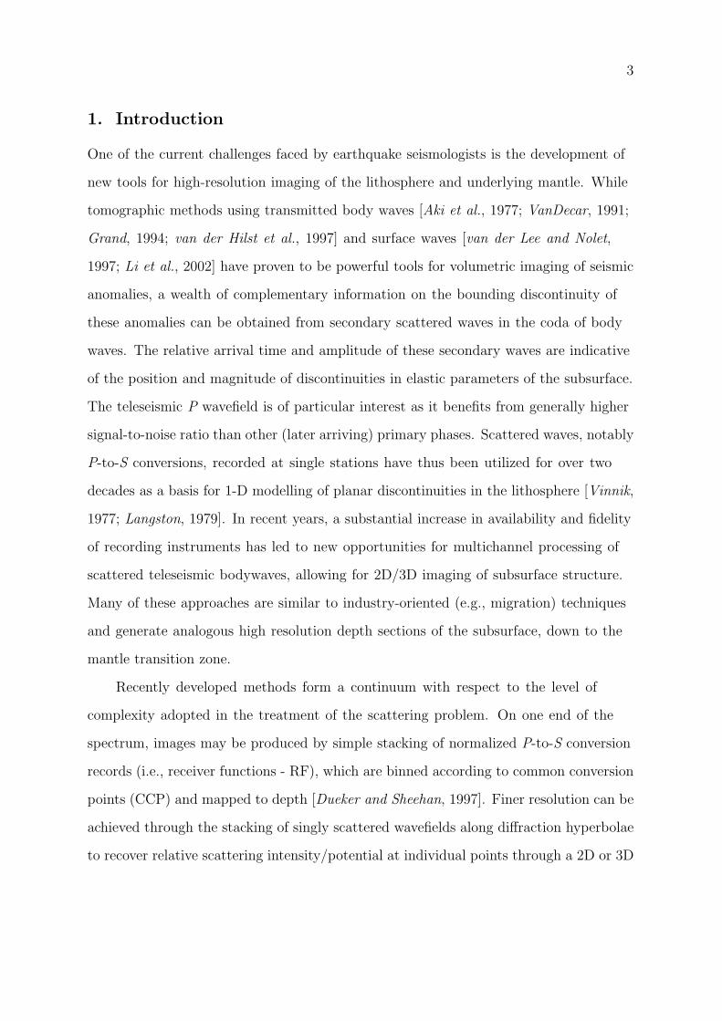
The forward problem, as expressed in Equation (1), is represented schematically

in Figure 1a for P-to-S transmission scattering. The scattered displacement observed

at a given time t and receiver position x′ in data space corresponds to the sum of

contributions from all scatterers x in model space that can generate signal at that data

point. These scatterers are distributed along an isochronal surface (i.e., t = T (x,x′,p0⊥)

constant) which is defined by the ray kinematics in the reference background model.

As originally recognized by Beylkin [1985], the scattered displacement field as

expressed in equation (1) possesses a form which closely resembles the Radon transform

in that it involves an integration over surfaces (or lines in 2D). This analogy with the

Radon transform (and its formal inverse) provides the basis for the development of a

back-projection operator to the scattering problem. The 2D Radon transform pair is

given by

F (n, s) =∫

dx f(x)δ(s− n · x), (3)

7

f(x0) = − 1

4π

∫dnH

[∂

∂sF (n, s)

∣∣∣∣∣s=n·x0

]

= − 1

4π

∫dn

∫dx f(x)H{δ′ [n · (x0 − x)]} (4)

= − 1

4π

∫ 2π

0dψ

∫dx f(x)H{δ′ [n · (x− x0)]} ,

where the surfaces of integration in (3) are planes defined by their normals n and their

distances from the origin s, angle ψ defines the direction of n, and H{·} denotes the

Hilbert transform. The definition of the inverse Radon transform in (4) indicates that

it is possible to reconstruct a function f(x) at any point x0 by summing F (n, s) over

all planes that pass through this point. Unlike the Radon transform, the isochronal

surfaces of integration in (1) are curved (see e.g., Figures 1a), but can be approximated

as planes when evaluating the integral in the vicinity of a point x0. A back-projection

operator for the scattering problem can be constructed by identifying ∆u(x′,p0⊥, t) with

F (n, s) in (4), with n and s corresponding to traveltime gradient ∇T and traveltime t,

respectively [see Miller et al., 1987]. This operator has the form:

f(x0, θ) =1

4π

∫dψ Y(x0,x

′,p0⊥)∆u[x′,p0

⊥, t = T (x0,x′,p0⊥)], (5)

where all weights and filters applied to the scattered displacement, including those

introduced to replicate the Radon transform, are grouped under the term Y(x0,x′,p0⊥).

Using equation (5) and the definition of the scattering potential f(x0, θ)

in (2), the material property perturbations at any scatter point in the model

∆m(x0)=[∆α/α0,∆β/β0,∆ρ/ρ0]T can be obtained by solving a small linear system,

leading to the expression

∆m = H−1g. (6)

Note that this system can be solved simultaneously for all scattering modes (i.e.,

forward- and back-scattering) and incident wavefields represented within a dataset. The

8

elements of g are given by

gl(x0) =1

4π

∫d∣∣∣p0⊥

∣∣∣ ∫ dγ∫

dx′1

∣∣∣∣∣ ∂(ψ, θ)

∂(x′1, γ)

∣∣∣∣∣Wl(θ)Y(x0,x′,p0⊥) ∆u[x′,p0

⊥, t = T (x0,x′,p0⊥)],

(7)

where γ = atan(p2/p01) is the event backazimuth. The determinant in the integrand of

equation (7) is a Jacobian (or “Beylkin determinant”) that permits practical integration

over variables representing source (|p0⊥|,γ) and receiver position x′ = (x′1, 0). The

elements of the Hessian matrix H are given by

Hlk(x0) =∫

d∣∣∣p0⊥

∣∣∣ ∫ dθWl(θ,∣∣∣p0⊥

∣∣∣ ,x0)Wk(θ,∣∣∣p0⊥

∣∣∣ ,x0). (8)

The inverse problem can, according to equations (7-8), be viewed simply as a

weighted diffraction stack over all sources and receivers (with weights determined by

the analogy with the Radon transform), followed by a trivial 3×3 matrix inversion. A

schematic representation of the inverse problem is displayed in Figure 1b for a single

incident wavefield. The inverse procedure is repeated for all image points in model space

to obtain a depth section of velocity and density perturbations.

2.2. Data preprocessing

Prior to inversion, the raw data must be preprocessed to effectively remove the incident

wavefield, thereby isolating the scattered displacement field (i.e., ∆u(x′,p0⊥, t)). This

preprocessing involves several steps which are presented in detail by Bostock and

Rondenay [1999], and can be summarized as follows (see Figure 2):

(1) Transform displacement u = [uR, uT , uZ ]T (where subscripts R, T and Z correspond

to radial, transverse and vertical directions, respectively) to an upgoing wave-vector

space w = [P, SC1, SC2]T using the inverse free-surface transfer matrix [Kennett,

1991]. This transformation isolates the incident P-wave to a single trace (P), with the

remaining two components (SC1,SC2) containing only scattered energy.

(2) Time-normalize (i.e. align) the resulting P-wave section using multi-channel

9

cross-correlation derived delay times [VanDecar and Crosson, 1990].

(3) Estimate and separate incident (I) and scattered (SC3) wavefields by principal

component (i.e., eigenimage) decomposition of the P-wave section [Ulrych et al., 1998].

I is obtained by reconstructing the section using only the first or first few principal

components, which represent that portion of the signal most strongly correlated from

trace to trace. SC3 is assembled using the remaining principal components, as an

estimate of the scattering contribution to the section.

(4) Reconstitute the upgoing scattered wavefield ∆uRTZ = [∆uR,∆uT ,∆uZ ]T from

w′ = [SC3, SC1, SC2]T using the using the eigenvector matrix for 1D media [e.g.,

Kennett, 1983].

(5) Deconvolve the estimated source-time function I from the reconstituted displacement

sections ∆uRTZ to obtain the scattered wave impulse response.

These first five steps lead to estimates of the scattered components of the Green’s

function ∆u(x′,p0⊥, t). Two additional steps are required to render the data sections

amenable to 2D GRT inversion:

(6) 2D treatment requires rotation of horizontal displacement into a reference frame

aligned with the inferred tectonic strike of the study area (i.e., x2 parallel to 2D regional

strike).

(7) Convolve the resulting data sections with the filter isgn(ω)/√−iω, which is included

in term Y(x0,x′,p0⊥) of equations (5) and (7), and is required through 2D GRT to

recover material property perturbations ∆m [see Bostock et al., 2001, their equation

(29)].

3. Resolution

The efficacy of 2D GRT inversion for the recovery of subsurface structure depends on

the combined effects of array and source configuration. As discussed in Bostock et al.

[2001], resolution is a measure of the accuracy in recovering both the geometry (depth,

10

volume and dip) of discontinuities and the amplitude of associated material property

perturbations. In this section, we consider several aspects of the theoretical framework

and applications to synthetic and field data to draw a set of basic observations and

guidelines regarding resolution.

3.1. Aperture - completeness of coverage

The analogy between forward/inverse scattering problems and the Radon Transform is

the fundamental basis of 2D GRT inversion. As discussed in detail by Bostock et al.

[2001], the validity of this analogy relies in large part on the coverage in total traveltime

gradient ∇T at each image point (see Figure 1). Specifically, the magnitude |∇T |

represents the sensitivity of traveltime to scatterer location, whereas its orientation

ψ controls dip resolution, such that structure dipping perpendicularly to sampling in

∇T will be well resolved. Volume resolution is controlled by the wave-number ω|∇T |,

where ω represents the angular frequency of the scattered signal [Bostock et al., 2001].

Therefore, a high degree of 2D spatial resolution will be insured by large values of |∇T |,

a large signal bandwidth, and complete directional coverage in ∇T (i.e., ψ=[-π/2,π/2]).

In practice, these conditions are only partially met for realistic field conditions. As a

result, geometrical resolution is reduced, causing distortion in the image. Moreover,

the recovery of accurate amplitudes of material property perturbations can be greatly

reduced, if not completely lost, if coverage is inadequate.

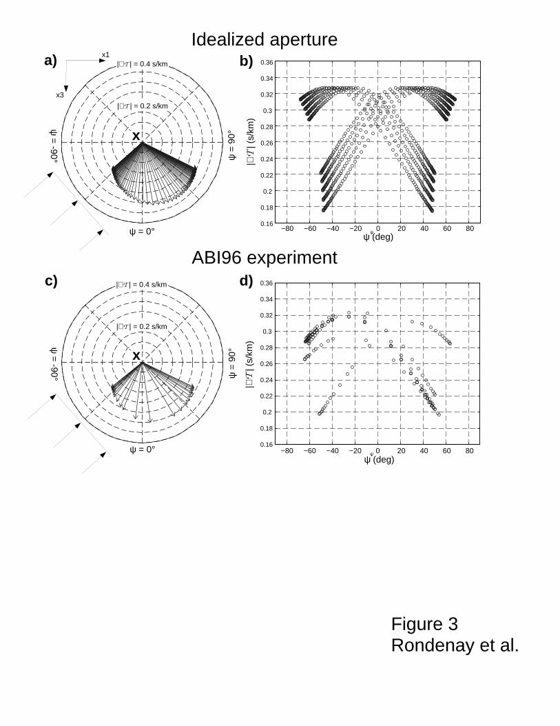
Figure 3 illustrates the sampling in ∇T achieved in an experimental setup for P-S

back-scattering at a single image point located at 40 km depth beneath the center of a

500km-long array. The top panels represent sampling in ∇T afforded by an idealized

station coverage (5 km uniform station spacing) for a single plane wave incident from

the left (Figure 3a), and incident waves from a full range of teleseismic distances [i.e.,

∼30-100◦] (Figure 3b). The lower panels show sampling at an image point beneath

the ABI96 array (irregular station spacing of ∼15-25km, see section 4.1) for an actual

11

event (Figure 3c) and the complete ray coverage afforded by the data set (Figure 3d).

Note that for single incident waves (i.e., left panels), the coverage in ∇T is represented

as vectors centered on the image point, whereas for complete ray coverage (i.e., right

panels) the values are plotted graphically. In the idealized case, the coverage in ψ is

nearly uniform over the range [-70◦,70◦], with all directions sampled by values of ∇T

> 0.32s/km. This is equivalent to the coverage that was afforded by the CASC93

data set [Rondenay et al., 2001], which produced realistic S-velocity perturbations of

±5% [see, also, Bostock et al., 2002]. The coverage afforded by the ABI96 data, on the

other hand, is much poorer in both ψ and |∇T |, with considerable gaps present in the

ψ=[-20◦,20◦] interval. The resulting loss of resolution and inability to recover exact

property perturbations is discussed in section 4.1. This type of analysis is useful to

assess the resolving power of 2D GRT inversion in different portions of model space as a

function of station and source coverage.

Lastly, we observe that for a fixed array width and complete range of teleseismic

incidences, the resolution tends to decrease with depth as the coverage in ∇T , and

especially the range in ψ, tend to diminish. Recalling the idealized example in

Figure 3a-b with an array width of 500 km, the range in ψ is reduced from [-70◦,70◦]

at 40 km depth to [-60◦,60◦] at 100 km and [-33◦,33◦] at 500 km. This implies that at

500 km depth, structure with dips greater than 33◦ will not be resolved. Provided that

the source distribution is complete and the sampling density is adequate, the main factor

controlling the geometrical resolution with increasing depth is array width. It is thus

possible to determine a maximum depth of resolution by choosing a minimum range in

ψ coverage for the center of the array. For example, with an average global model, a

range of [-45◦,45◦] will be reached at a depth equivalent to approximately half the array

width. Note, however, that moving the image point toward the edge of the model tends

to reduce the ψ range and shift its mean value. Accordingly, at a depth corresponding

to half the array width, we find that ψ ∼[-60◦,15◦] on the left [i.e., min(x1)] side of the

12

model and ψ ∼[15◦,-60◦] on the right side [i.e., max(x1)].

3.2. Spatial Aliasing

The surface density of recording instruments determines, in large part, the quadrature

employed for solving the integral in the GRT inverse operator (see equation 4). It is a

crucial factor affecting the resolving power of 2D GRT inversion, as it controls spatial

sampling of the scattered signal. Indeed, as abundantly reported by the active source

community [e.g., Yilmaz, 1987], a degradation in geometrical resolution arises when

applying imaging/migration operators to signal that is spatially undersampled (i.e.,

aliased).

Spatial aliasing will occur when station density at the surface is such that the

incoming scattered wavefield is sampled at intervals greater than half its apparent

wavelength λ. For the simple case of a plane wave traveling through a homogeneous

half-space, it can be shown [e.g., Yilmaz, 1987] that the station spacing required to

avoid aliasing approaches asymptotically λ/2 for horizontal incidence. Assuming an

average crustal S-velocity of 3.6 km/s, this means that station spacing must be no larger

than 1.8-18 km to adequately sample signal with dominant frequency ranging over the

interval 1-0.1 Hz. Spatial aliasing considered in these terms will thus affect the images

obtained with 2D GRT inversion if the station density is too sparse. However, the

negative effects of aliasing will be offset, in part, by the broad signal bandwidth of the

teleseismic P-wavefield and the simultaneous processing of multiple incident waves and

scattering modes.

In the specific case of 2D GRT inversion, there is another aliasing prob-

lem which is related to undersampling of GRT-derived stacking weights (i.e.,

14π

∣∣∣ ∂(ψ,θ)∂(x′1,γ)

∣∣∣Wl(θ)Y(x0,x′,p0⊥) in equation 7). Applications to sparsely sampled synthetic

data [Shragge et al., 2001] and field data (section 4.1) show that this type of stacking

parameter aliasing is manifested through a high wave number “speckle” in the resulting

13

image. These effects, however, tend to be predominant near the surface and diminish

with increasing depth. This behaviour is related to rapid variations in traveltime

sensitivity ∇T near the surface, which produce sharp peaks in the total weighting

function of the diffraction hyperbola. A high spatial density of data in thus necessary

to adequately sample these peaks. As depth increases, however, the weighting function

becomes smoother and can be better sampled by sparser recording points. This form

of aliasing is illustrated in Figure 4, which shows the total weighting function for

P-S backscattering at an image point located at increasing depth, in the center of a

500 km-long array. The appearance of the weighting function is shown for various

sampling densities (continuous, 5 km and 20 km station spacing). This test suggests

that for an average global model (e.g., IASP91, Kennett and Engdahl [1991]), stacking

weight aliasing should affect the resulting image between the surface and a depth

approximately equivalent to twice the station spacing. Caution should thus be taken

when interpreting images in this depth range.

3.3. Model space assumptions

In addition to the direct effects from source and station distribution, the resolution

afforded by 2D GRT inversion may also be affected by departures from assumptions

adopted in its theoretical development. In this section, we briefly discuss the implications

of three such assumptions, namely the Born approximation, isotropy, and 2D geometry.

The Born approximation permits the linearization of the forward problem through

the assumption that all wave propagation occurs through the unperturbed reference

medium. This assumption is valid while the scattered component of the total wavefield

remains much smaller than the unperturbed wavefield. Detailed criteria for the validity

of the Born approximation in seismic scattering can be found in Hudson and Heritage

[1981]. Generally, material property perturbations should remain small (i.e., ∆α� α0,

∆β � β0, ∆ρ� ρ0) and the scale length of the scattering bodies should not exceed the

14

dominant wavelength of the signal. Violation of these assumptions results in two main

complications. First, it allows for significant multiple scattering to occur, which may

result in the inclusion of artificial structure in the final image. Second, it modifies the

predicted ray kinematics of the wavefield and thereby produces an incomplete focusing

of scattered signal.

The 2D GRT inversion assumes that the scatterers and background reference model

display isotropic elastic properties. This is a convenient and commonly used assumption,

as it reduces the number of independent inversion parameters to three unknowns

(e.g., ∆α/α0, ∆β/β0, and ∆ρ/ρ0). However, as extensively reported in the literature

[see Fischer et al., this volume], many types of mineral assemblages and structural

features comprised in the crust and underlying mantle display strong coherent fabric

that result in directional variations of elastic properties (i.e., anisotropy). The presence

of anisotropy, if unaccounted for, may affect 2D GRT inversion images in two main

ways: (1) structures will be mismapped and defocused due to altered ray kinematics

[see, e.g. Larner and Cohen, 1993; Tsvankin, 1996]; (2) recovery of material property

perturbations will be compromised due to the computation of incorrect radiation

functions for the scattered waves [see Burridge et al., 1998]. A better characterization

of anisotropic scattering parameters requires significant modifications to the current

methodology, as discussed in section 5.

Lastly, the main reason for adopting a 2D formulation of the scattering problem is

the limitation in currently available instrumentation, which precludes the deployment of

seismometers over very dense grids necessary for a general 3D approach (see section 5

for a discussion on this matter). The 2D treatment may often be an oversimplifying

assumption, yet it has been successfully used for many years in the oil industry [see,

e.g., Yilmaz, 1987] and in crustal studies [e.g., Clowes et al., 1992]. Departure from this

assumption may result in the inclusion of coherent signal from out-of-plane plane 3D

scatterers in the final image. This signal will not necessarily map constructively but it

15

will increase the level of background noise. It is thus important to test the validity of

our approach by computing the minimum out-of-plane extent of 2D structure required

to satisfy the assumption, and by comparing this value with information from regional

tectonic models. Figure 5 presents a set of minimum values calculated for a global

average model (i.e., iasp91) as a function of scatterer’s depth and horizontal in-plane

distance from the recorder.

4. Applications to field data

In this section, we apply 2D GRT inversion to data from two IRIS-PASSCAL

experiments, ABI96 and LARSE. The main objective of this exercise is to assess the

applicability of the method to deployments that do not meet its explicit geometrical or

data requirements. In the case of ABI96, station coverage is relatively sparse (∼20 km)

and the data exhibit significant contamination by coherent noise and unwanted

teleseismic arrivals. For the LARSE array, the data are more densely sampled (∼2 km)

but they were recorded by short-period instruments, limiting the bandwidth of the

recovered scattered signal. For an assessment of the full potential of 2D GRT inversion,

the reader is referred to a previous application of the method to field data from the

CASC93 experiment [see Rondenay et al., 2001; and Bostock et al., 2002].

4.1. ABI96 field data

During the summer of 1996, a portable array comprising 28 broadband three-component

seismometers was deployed across the SE Canadian Shield, with an average station

spacing of 20 km. The array followed the main axis of the Lithoprobe Abitibi-Grenville

transect [Ludden and Hynes, 2000], sampling Archean terranes of the Superior Province

to the NW and Proterozoic rocks of the Grenville Province to the SE (Figure 6a).

Results from a receiver function profile along this array were reported in Rondenay et al.

[2000], and are reproduced here in Figure 6e. The colour scale represents the amplitude

16

of the normalized impulse responses, with red and blue pulses denoting discontinuities

with positive and negative downward velocity gradients, respectively. Starting from the

southern end of the profile, Moho topography is apparent with northwestward crustal

thickening from 40 to 45 km, followed by an abrupt thinning of ∼10km occurring some

65km south of the Grenville Front (GF). This jump was interpreted as the signature of

a suture zone complex, with the GF representing the surface expression of an associated

crustal ramp. The presence of relict subducted crust in the Superior cratonic lithosphere

is suggested by a sequence of negative polarity arrivals projecting northward into the

mantle from the Moho step.

Two important issues regarding preprocessing must be considered before applying

2D GRT inversion to this data set. The first is data selection. Figure 6b shows the

locations of the 49 events selected to generate the 568 receiver functions used in the

study of Rondenay et al. [2000]. The authors employed the simultaneous deconvolution

algorithm of Bostock [1998], followed by mapping of time to depth. This process is

loosely equivalent to a 1D post-stack migration operator and tends to enhance coherent

signal related to continuous, sub-horizontal discontinuities relative to locally scattered

signal or noise. Consequently, signal-to-noise ratio requirements are not as stringent as

those of 2D GRT inversion, a form of pre-stack migration that tends to carry the noise

constructively into the final image. Due to these restrictions, only 7 of the original 49

events were retained for the inversion (see Figure 6b).

The second issue regarding preparation of the ABI96 data is a recurrent problem

of P-coda contamination by later arriving body-waves. Specifically, 3 of the 7 selected

events were located within 45-65◦ distance from the array center, a distance range where

teleseismic PcP has high amplitude and pronounced moveout from P, which it trails by

100-30 s. This time difference results in the introduction of unwanted coherent PcP

signal in that portion of the P-coda which is sampled for scattered energy in the top

250 km of the model, thereby causing artificial structure in the resulting image. The

17

same problem arises with teleseismic PP when attempting to image sublithospheric

structure that require extended (∼300 s) data sections. In order to resolve this

contamination problem, a series of preprocessing steps in addition to those in section 2.2

are implemented. These steps are applied prior to deconvolution of the scattered

wavefield and can be summarized as follows: (i) the traveltime and horizontal slowness

of the corrupting phase is identified and (ii) its waveform is isolated using the inverse

free surface transfer matrix; (iii) the traces are optimally aligned with respect to this

phase using multichannel cross-correlation; (iv) a principal component decomposition

is applied and the first principal component, which contains the corrupting phase, is

effectively extracted from the section; and (v) a clean data set is recovered by realigning

the traces with respect to P and multiplying by the free-surface transfer matrix. This

preprocessing sequence removes most of the unwanted signal, as illustrated in the

example of Figure 6c-d. It is important to note, however, that this procedure will also

remove coherent scattered energy that displays the same moveout and polarization as

the unwanted phase.

The 2D GRT inversion was applied to the preprocessed and decontaminated records

from the seven selected events. Figure 6f shows the resulting S-velocity perturbation

profile, with red to blue colour scale representing negative (slower) to positive (faster)

velocity perturbations. In this type of profile, velocity discontinuities are thus denoted

by colour contrasts (i.e., red-to-blue or blue-to-red). We note that the quality of

the final image is remarkably high given the limited number of events retained for

analysis. The Moho appears as a strong discontinuity that closely follows topographical

variations observed on the RF profile (Figure 6e). It is important to note that whereas

the RF image does not exploit free-surface multiples, the 2D GRT inversion relies

primarily on these backscattered signals [see Shragge et al., 2001; Rondenay et al., 2001].

Consequently, there is a large degree of independence between the two images. The

2D GRT inversion also images a complex structure near the previously imaged Moho

18

step. However, the feature in Figure 6f appears as less of a step and more as a series of

imbricated ramps. Given the limited source/station distribution, it is difficult to assess

whether this complex structure is real or if it is an artifact due to reduced coverage in

∇T in the SE portion of the array.

We further note that 2D GRT inversion detects a possible discontinuity projecting

into the mantle from the Moho disruption. This structure is better defined and possesses

a greater dip (∼22◦) than that observed in the RF profile. The dip is well within the

range of dip resolution of [-55◦,60◦], which is afforded by the complete ABI96 dataset in

this portion of the model (i.e., x1=300km, x3=80km). The mantle feature in Figure 6f

is expected to be more robust, as 2D GRT inversion is more effective at constructively

summing scattered signal emanating from dipping interfaces. However, greater source

coverage would be required to better constrain this feature.

The resolution of the final image (Figure 6f) is affected by two of the factors

discussed in section 3. First, the large station spacing places the top portion of the

model in the region affected by stacking weight aliasing. According to the rule of thumb

devised in section 3.2, the affected region should extend between 0-40 km depth (i.e.,

twice the station spacing). In the present case, aliasing results in a high wave-number

“speckle” which distorts the image mostly between 0-20 km depth. This implies that

the predicted extent of the affected region can be reduced, in part, by the simultaneous

treatment of multiple sources. Second, due to the incomplete and irregular coverage

in ∇T at each image point (see Figure 3d), the magnitudes of material property

perturbation (i.e., δβ/β0 in Figure 6f) are not correctly recovered. Therefore, when

dealing with limited data sets, the resulting profiles should be interpreted strictly as

scattering potential images.

In summary, this application of 2D GRT inversion demonstrates that while sparse

data sampled at ∼20 km intervals may not be ideal for this type of analysis, they

still display a clear potential for imaging structure in the lower crust and underlying

19

lithospheric mantle.

4.2. LARSE field data

During the fall of 1993, a linear array of 89 vertical and three-component short-period

seismometers was deployed across the Los Angeles Basin, San Gabriel Mountains and

Mojave Desert, as part of the LARSE experiment (Figure 7a). The array was 175 km

long with a ∼2 km station spacing, and it was designed to perpendicularly intersect

2D regional structure, in particular the San Andreas Fault. A receiver function profile

beneath this array was produced by Zhu [2000] using 941 traces (from 30 events) binned

according to Common Conversion Points. This study identified abrupt vertical offsets

in Moho depth occurring directly beneath the surface location of the San Andreas Fault

and the Eastern California Shear Zone. These results support a thick-skinned behaviour

for these two crustal structures.

We introduce this data set to demonstrate two important issues in imaging

lithospheric structure using teleseismic body-wave data, namely the contaminating

influences of unmodelled scattering and errors in the estimated source time function. In

Figure 7c we show the result of preprocessing only vertical component seismograms to

produce an estimate of the scattered wavefield. Partly coherent signals with hyperbolic

moveout are evident and centered near distance 43 km. At first glance this observation

is encouraging as it suggests the presence of strong localized subsurface heterogeneity.

However, closer examination indicates that the apparent velocity of these signals is

approximately 3.2 km/s. As the true wave velocity can only be less than the apparent

velocity, this energy most likely represents Rayleigh waves originating through scattering

from off-axis, surface topography. This inference is supported by a plot of surface

topography along the profile wherein it is noted that the hyperbola apices coincide

closely with the maximum in topography and topographic gradient (Figure 7c). The

particle motions of Rayleigh waves also project onto the horizontal components and it

20

is therefore important to assess and minimize their effect on images of the immediately

underlying San Andreas fault as produced using more traditional receiver function

approaches [Zhu, 2000; see further discussion in section 5].

The image resulting from inversion of the short-period vertical component data

from 9 events (see Figure 7b) are shown in Figure 7d. There is little in the image that

can be confidently attributed to major lithospheric structure. In particular, the Moho,

which is evident in images [e.g., Zhu, 2000] that incorporate horizontal component

(i.e., S-wave) information, cannot be identified using free-surface P-wave multiples.

The primary reason for this is that our source estimation procedure is ineffective in

distinguishing signal generated by near-horizontal planar structure from complexity in

the source time function. The resulting errors in the source-time function have a much

larger effect on P-wave data than S-wave data because the P-wave data are dominated

by the incident wave whereas S-wave data contain, by definition, only scattered wave

energy.

In summary, this example demonstrates that there are outstanding factors that

compromise the use of 2D GRT inversion on short-period, vertical component data sets.

Therefore, application of the method in its present form is not recommended for this

category of experimental setup. Nevertheless, possible future improvements discussed in

the next section may change this situation.

5. Future directions

We now build on our understanding of the factors affecting resolution to discuss a

series of improvements that may render the GRT inversion approach more robust and

more generally applicable. Five main points are considered.

First, the GRT inversion could be readily implemented for 3D isotropic scattering.

This would permit better focusing of signal scattered at realistic subsurface structure.

The theory has already been developed for the acoustic [Miller et al., 1987] and elastic

21

[Beylkin and Burridge, 1990] treatment of seismic reflection data. The only caveat to 3D

GRT inversion lies in the considerable, and thus prohibitive requirements for recording

instruments. For example, a grid of 225 recording nodes (equipped with broadband

seismometers) would be necessary to image a region of 300 km×300 km with an average

station spacing of 20 km.

Second, the approach can be made more general by considering the inverse

scattering problem for an anisotropic, elastic medium. Such anisotropic approaches

have already been implemented by Burridge et al. [1998] for seismic reflection data,

and by Bostock [2002] and Bank and Bostock [2002] for the 1D teleseismic case. The

main challenge with generalization to an anisotropic medium lies in the large number of

independent perturbations that are inverted for. There are 22 independent parameters

in the most general case, comprising 21 elastic tensor components plus density. Note,

however, that this number is reduced to 9+1 parameter for orthorhombic systems (e.g.,

olivine) and to 5+1 for hexagonal symmetry. Given the limited source-receiver coverage,

the problem is generally underdetermined and only linear combinations of anisotropic

parameters can be recovered [Burridge et al., 1998]. Furthermore, it is not obvious that

the data sampling and signal-to-noise levels afforded by teleseismic waves will generally

be sufficient to contemplate fully 3D inversion for anisotropic structure. Nevertheless,

this type of analysis would prove useful in estimating the fraction of the scattered signal

that can only be explained by anisotropic perturbations.

Third, as we have noted from our analysis of the LARSE data set, unmodelled

teleseismic body-to-surface wave scattering [Revenaugh, 1995b; Abers, 1998] poses

a serious impediment to the utilization of higher frequency data in resolving fine

scale structure. This form of scattering is most severe at short periods (<2s). From

the observations we have made to date in subduction zones [e.g., Rondenay et al.,

2001], there is apparently a mid-period band (3-10 s, accessible using broadband

instrumentation) wherein scattering is largely coherent and relatively unaffected by

22

topography. Extending the useful band to still higher frequencies may be possible

by developing 3D generalizations of the 1D free-surface forward and inverse transfer

operators [Kennett, 1991; Bostock and Rondenay, 1999] employed in the present work.

Using densely sampled topographic data bases, it may thereby be possible to attenuate

surface wave signals in the preprocessing sequence.

Fourth, estimation of the source-time function is another area of research where

improvements are needed if structural information from intra-mode (e.g., P-to-P, S-to-S)

scattering is to be extracted. Our use of principal component analysis to attempt

separation of incident and scattered wavefields fails to accurately separate low-frequency

scattered signal from near-horizontal, planar structure. As a result, the Moho, for

example, is generally not identifiable on images constructed from free-surface P-to-P

multiples. It is possible that this problem can be overcome by exploiting contrasting

statistical properties of the source and scattering to better accomplish their separation.

Finally, it would be desirable to move beyond the Born or single-scattering

approximation in teleseismic imaging. The effect of this assumption is manifest in

two ways. Firstly, if the background medium does not accurately capture the long

wavelength components of the true Earth’s velocity, imaged structure will be distorted

and mispositioned. Better estimates of large-scale velocity structure can be achieved

through contemporaneous tomographic analysis of the traveltimes of direct waves.

Alternatively, newly developed approaches [Weglein et al., 2002] that exploit higher

order terms in the Born and inverse scattering series may be viable. However, these

approaches rely heavily on an accurate knowledge of scattered wave amplitudes that

may be difficult to achieve in practical circumstances.

A second consequence of the single-scattering approximation is the appearance

of image artifacts related to discrete, multiply scattered arrivals. These include most

notably free-surface multiples. Our 2D GRT approach partially accounts for the

free-surface multiples by considering them as generated by image sources located above

23

the free-surface and incorporating them within the inversion. However, because we

do not isolate each different multiple mode into separate data sections, they cross

contaminate one another in the resulting images [Shragge et al., 2001]. The machinery

afforded by the Born/inverse scattering series [Weglein et al., 1997] may provide a

means of isolating individual data sections corresponding to each free-surface multiple

as part of the preprocessing sequence. The individual data sections can then be inverted

simultaneously to produce images which do not possess cross-mode contamination. This

approach is currently a topic of investigation.

6. Conclusions

Until now, the 2D GRT inversion presented in Bostock et al., [2001] has only been

applied to ideal synthetic and field data that are not necessarily representative of

characteristic experimental setups. In this paper, we have assessed the resolving power

of the approach for variable field conditions. In particular, we demonstrated that: (1)

comprehensive source/station coverage is necessary to optimize geometrical resolution

and recover accurate material property perturbations; (2) the range in dip resolution

diminishes with increasing depth and is inversely proportional to array width (e.g.,

reaches [-45◦,45◦] at depths equivalent to ∼1/2 array width); (3) distortion of the

image due to spatial aliasing is only significant at depths ≤2×[station spacing]; and (4)

unaccounted for departures from model assumptions (smooth variations, isotropy, and

2D geometry) result in defocusing and mismapping of structure.

We have further illustrated the potential and limitations of 2D GRT inversion

through two new applications to field data. Application to ABI96 required the

introduction of additional preprocessing steps to minimize contamination of the data by

PcP and PP waves. Results demonstrated that structure from the lower crust downward

could be successfully imaged by broadband data from relatively sparse seismic arrays

with ∼20 km station spacing. Limited source distribution was shown to hinder the

24

recovery of accurate material property perturbations, but the resulting images could still

be interpreted in terms of more general scattering potentials. Application to LARSE

showed that images obtained from high frequency records were subject to significant

contamination by scattered surface waves. Further decrease in resolution was attributed

to a loss of scattered signal through the preprocessing steps currently used to render the

data amenable to analysis. The development of improved preprocessing tools that could

isolate the different scattering modes from the incident wavefield and corrupting phases

is the focus of ongoing research.

Acknowledgments. This work was supported by an NSERC postdoctoral fellowship to

SR.

25

References

Abers, G., Array measurements of phase used in receiver-functions calculations: importance

of scattering, Bull. Seismol. Soc. Am., 88, 313-318, 1998.

Aki, K., A. Christofferson, and E. S. Husebye, Determination of the three-dimensional seismic

structure of the lithosphere, J. Geophys. Res., 82, 277-296, 1977.

Bank, C.-G., and M. G. Bostock, Linearized inverse scattering of teleseismic waves for

anisotropic crust and upper mantle structure, II. Numerical examples and applications

to data from Canadian stations, submitted to J. Geophys. Res., 2002.

Beylkin, G., Imaging of discontinuities in the inverse scattering problem by inversion of a

causal generalized Radon transform, J. Math. Phys., 26, 99-108, 1985.

Beylkin, G., and R. Burridge, Linearized inverse scattering problem by inversion of a causal

generalized Radon transform, Wave Motion, 12, 15-52, 1990.

Bostock, M. G., Mantle stratigraphy and evolution of the Slave province, J. Geophys. Res.,

103, 21,183-21,200, 1998.

Bostock, M. G., and S. Rondenay, Migration of scattered teleseismic body waves, Geophys. J.

Int., 137, 732-746, 1999a.

Bostock, M. G., and S. Rondenay, Corrigendum to “Migration of scattered teleseismic body

waves”, Geophys. J. Int., 139, 597, 1999b.

Bostock, M. G., S. Rondenay, and J. Shragge, Multiparameter two-dimensional inversion of

scattered teleseismic body waves, 1, Theory for oblique incidence, J. Geophys. Res.,

106, 30,771-30,782, 2001.

Bostock, M. G., Kirchhoff-approximate inversion of teleseismic wavefields, Geophys. J. Int.,

149, 787-795, 2002.

Bostock, M. G., R. D. Hyndman, S. Rondenay, and S. M. Peacock, An inverted continental

Moho and serpentinization of the forearc mantle, Nature, 417, 536-538, 2002.

Bostock, M. G., Linearized inverse scattering of teleseismic waves for anisotropic crust and

upper mantle structure, I, Theory, submitted to J. Geophys. Res., 2002.

Burridge, R., M. V. de Hoop, D. Miller, and C. Spencer, Multiparameter inversion in

26

anisotropic elastic media, Geophys. J. Int., 134, 757-777, 1998.

Clowes, R. M., F. A. Cook, A. G. Green, C. E. Keen, J. N. Ludden, J. A. Percival, G. M.

Quinlan, and G. F. West, Lithoprobe: new perspectives on crustal evolution, Can. J.

Earth Sci., 29, 1813-1864, 1992.

Dueker, K. G., and A. F. Sheehan, Mantle discontinuity structure from midpoint stacks of

converted P to S waves across the Yellowstone hotspot track, J. Geophys. Res., 102,

8313-8327, 1997.

Grand, S. P., Mantle shear structure beneath the Americas and surrounding oceans, J.

Geophys. Res., 99, 11591-11621, 1994.

Hudson, J. A., and J. R. Heritage, The use of the Born approximation in seismic scattering

problems, Geophys. J. Roy. Astr. S., 66, 221-240, 1981.

Kennett, B. L. N., Seismic wave propagation in stratified media, Cambridge University Press,

Cambridge, UK, 1983.

Kennett, B. L. N., The removal of free surface interactions from three-component seismograms,

Geophys. J. Int., 104, 153-163, 1991.

Kennett, B. L. N., and E. R. Engdahl, Travel times for global earthquake location and phase

identification, Geophys. J. Int., 105, 429-465, 1991.

Langston, C. A., Structure under Mount Rainier, Washington, inferred from teleseismic body

waves, J. Geophys. Res., 84, 4749-4762, 1979.

Larner, K. L., and J. K. Cohen, Migration error in transversely isotropic media with linear

velocity variation with depth, Geophysics, 58, 1454-1467, 1993.

Levander, A., E. Humphreys, G. Ekstrom, A. Meltzer, and P. Shearer, Proposed project would

give unprecedented look under North America, Eos Trans. AGU, 80, 245, 1999.

Li, A., D. W. Forsyth, and K. M. Fischer, Shear wave structure and azimuthal anisotropy

beneath eastern North America, submitted to J. Geophys. Res., 2002.

Ludden, J., and A. Hynes, The Lithoprobe Abitibi-Grenville transect: two billion years of

crust formation ad recycling in the Precambrian Shield of Canada, Can. J. Earth Sci.,

37, 459-476, 2000.

Miller, D., M. Oristaglio, and G. Beylkin, A new slant on seismic imaging: Migration and

27

integral geometry, Geophysics, 52, 943-964, 1987.

Revenaugh, J., A scattered-wave image of subduction beneath the Transverse Ranges, Science,

268, 1888-1892, 1995a.

Revenaugh, J., The contribution of topographic scattering to teleseismic coda in Southern

California, Geophys. Res. Lett., 22, 543-546, 1995b.

Rondenay, S., M. G. Bostock, T. M. Hearn, D. J. White and R. M. Ellis, Lithospheric assembly

and modification of the SE Canadian Shield: Abitibi-Grenville Teleseismic Experiment,

J. Geophys. Res., 105, 13,735-13,754, 2000.

Rondenay, S., M. G. Bostock, and J. Shragge, Multiparameter two-dimensional inversion of

scattered teleseismic body waves, 3, Application to the Cascadia 1993 data set, J.

Geophys. Res., 106, 30,795-30,808, 2001.

Ryberg, T., and M. Weber, Receiver function arrays: a reflection seismic approach, Geophys.

J. Int., 141, 1-11, 2000.

Sheehan, A. F., P. M. Shearer, H. J. Gilbert, and K. G. Dueker, Seismic migration processing

of P-SV converted phases for mantle discontinuity structure beneath the Snake River

Plain, western United States, J. Geophys. Res., 105, 19055-19065, 2000.

Shragge, J., M. G. Bostock, and S. Rondenay, Multiparameter two-dimensional inversion

of scattered teleseismic body waves, 2, Numerical examples, J. Geophys. Res., 106,

30,783-30,794, 2001.

Tsvankin, I., P-wave signatures and notation for transversely isotropic media: An overview,

Geophysics, 61, 467-483, 1996.

Ulrych, T. J., M. D. Sacchi, and S. L. M. Freire, Eigenimage processing of seismic sections, in

Covariance Analysis of Seismic Signal Processing, edited by R. L. Kirlin, and W. J.

Done, SEG Monograph, Tulsa, 1998.

VanDecar, J. C., Upper-mantle structure of the Cascadia subduction zone from non-linear

teleseismic travel-time inversion, Ph.D. thesis, 165 pp., Univ. of Wash., Seattle, June

1991.

VanDecar, J. C., and R. S. Crosson, Determination of teleseismic relative phase arrival times

using multi-channel cross-correlation and least squares, Bull. Seismol. Soc. Am., 80,

28

150-159, 1990.

van der Hilst, R. D., S. Widiyantoro, and E. R. Engdahl, Evidence for deep mantle circulation

from global tomography, Nature, 386, 578-584, 1997

van der Lee, S., and G. Nolet, Upper mantle S velocity structure of North America, J.

Geophys. Res., 102, 22,815-22,838, 1997.

Vinnik, L. P., Detection of waves converted from P to SV in the mantle, Phys. Earth Planet.

Inter., 15, 39-45, 1977.

Weglein, A. B., F. A. Gasparatto, P. M. Carvalho, and R. H. Stolt, An inverse-scattering series

method for attenuating multiples in seismic reflection data, Geophysics, 62, 1975-1989,

1997.

Weglein, A. B., D. J. Foster, K. H. Matson, S. A. Shaw, P. M. Carvalho, and D. Corrigan,

Predicting the correct spatial location of reflectors without knowing or determining

the precise medium and wave velocity: Initial concept, algorithm and analytic and

numerical example, J. Seism. Explor., 10, 367-382, 2002.

Wessel, P., and W. H. F. Smith, New version of the Generic Mapping Tools released, Eos

Trans. AGU, 76, 329, 1995.

Yilmaz, O., Seismic data processing, Society of Exploration Geophysicists, Tulsa, OK, 1987.

Zhu, L., Crustal structure across the San Andreas Fault, southern California from teleseismic

converted waves, Earth Planet. Sc. Lett., 179, 183-190, 2000.

Received xx, yyyy; revised xx, yyyy; accepted xx, yyyy.

1Department of Geological Sciences, Brown University, Providence, Rhode Island, USA.

2Department of Earth and Ocean Sciences, University of British Columbia, Vancouver,

British Columbia, Canada.

29

Figure 1. Schematic representation of forward and inverse scattering problems for P-

to-S scattering in terms of model space (i.e., scatterer location) and data space (i.e.,

station position versus time). a) Forward problem expresses the scattered displace-

ment field measured at a given time t = T (x,x′,p0⊥) and station location x′, due to

all point scatterers in model space that could contribute energy to that point in data

space. b) Inverse problem involves weighted diffraction stack along the travel-time curves

corresponding to a point scatterer at x and recovers material property perturbations

∆ml=(∆α/α0,∆β/β0,∆ρ/ρ0) at that point (shown here for a single source).

Figure 2. Preprocessing of the P-coda from a Mexico earthquake (Sept. 3, 1993;

12:35:00 UT; 14.52◦N, -92.71◦E, 27 km; mb=5.8) recorded at station A03 (44.42◦N,-

123.95◦E) of the CASC93 deployment. Seismic traces represent, from top to bottom:

radial, transverse and vertical components of the raw data (uR, uT , uZ ); decomposed P-,

SC1- and SC2- components; estimates of the incident (I) and scattered (SC3) wavefields

determined from principal component analysis; scattered displacement field in the x1, x2

and x3 directions, bandpass filtered between 0.03-0.3 Hz (∆u1 ,∆u2 ,∆u3 ).

Figure 3. Aperture (i.e., coverage in ∇T ) as a function of station and source distribu-

tion, for a single image point located at 40 km depth beneath the center of a 500km-long

array. Top panels: idealized scenario with 5 km station spacing for (a) a single plane wave

incident from the left on image point x (see Figure 1 for description of x1-x3 axes), and

(b) incident waves at a full range of teleseismic distances (i.e., ∼30-100◦). Lower panels:

image point beneath the ABI96 array (see section 4.1) with irregular station spacing of

∼15-25km for (a) a single plane wave incident from the left, and (b) the complete ray

coverage afforded by the data set.

30

Figure 4. Sampling of the weighting function applied to the diffraction stacks, for a

single image point located at (a) 2 km, (b) 10 km, (c) 25 km, and (d) 50 km beneath

the center of a 500km-long array. The thick gray line represents continuous sampling,

whereas solid and dashed black lines represent sampling at 5 km and 20 km, respectively.

Undersampling is manifest to depths equivalent to approximately 2×[station spacing].

Figure 5. Minimum out-of-plane extent of 2D scatterer required by model-space as-

sumptions, as a function of scatterer’s depth (∆x3) and horizontal in-plane distance

from recorder (∆x1).

Figure 6. ABI96 experiment. a) Map of the study area. b) Distribution of events se-

lected for receiver function analysis (green squares) and 2D GRT inversion (red circles).

c) Scattered P-wavefield section obtain through preprocessing steps described in sec-

tion 2.2. Note the contamination by teleseismic PcP and PP waves. d) Decontaminated

P-wavefield section. e) Receiver function profile. Red and blue pulses denote disconti-

nuities with positive and negative downward velocity gradients, respectively. Black lines

show interpretation. Abbreviations: GF = Grenville Front, M = Moho. f) S-velocity

perturbation profile obtained by 2D GRT inversion, with red to blue colour scale repre-

senting negative (slower) to positive (faster) velocity perturbations.

Figure 7. LARSE experiment. a) Map of the study area. Abbreviations: SAF = San

Andreas Fault, ECSZ = Eastern California Shear Zone. b) Distribution of events selected

for 2D GRT inversion. c) Top panel: surface topography along the profile. Lower panel:

scattered P-wavefield section for a Kamchatka earthquake (Nov. 17, 1993; 11:18:50 UT;

51.79◦N, 158.67◦E, 24 km; mb=6.1). Note the presence of coherent diffractions hyperbolas

centered near distance 43 km, coinciding closely with maximum in topography. d) P-

velocity perturbation profile obtained by 2D GRT inversion, with colour scale defined as

for Figure 6f.

✱∆α∆β∆ρ{

FORWARD PROBLEMHorizontal distance - x1 [km]

Tim

e -

t [s]

Dep

th -

x3 [

km]

Tim

e -

t [s]

Dep

th -

x3 [

km]

Horizontal distance - x1 [km] Horizontal distance - x1 [km]

INVERSE PROBLEM

Horizontal distance - x1 [km]

➧

➧

✱

a)

b)

x

x′ T (x′,T (x′,x,p )0

⊥t =

x′

x′ x′

x

p 0⊥

T (x′,x,p )0⊥

p 0⊥

x,p ) 0⊥

=const ant ψ

T (x′,x,p )0⊥∇

Figure 1Rondenay et al.

0 10 20 30 40 50 60Time [seconds]

PSC1SC2

I

SC3

uR

uT

uZ

∆u1

∆u2

∆u3

Data preprocessing

Figure 2Rondenay et al.

τP

ψψ (deg)

|∇T

| (s/

km)

x3

x1

Idealized aperture

ABI96 experiment

Figure 3Rondenay et al.

a) b)

0.16

0.18

0.2

0.22

0.24

0.26

0.28

0.3

0.32

0.34

0.36

−80 −60 −40 −20 0 20 40 60 80

−80 −60 −40 −20 0 20 40 60 800.16

0.18

0.2

0.22

0.24

0.26

0.28

0.3

0.32

0.34

0.36

ψψ (deg)

c) d)

|∇T

| (s/

km)

ψ =

90°

ψ = 0°

ψ =

-90°

ψ =

90°

ψ = 0°

ψ =

-90°

|∇T | = 0.2 s/km

|∇T | = 0.4 s/km

|∇T | = 0.2 s/km

|∇T | = 0.4 s/km

x

x

Horizontal distance [km]

Tot

al W

eigh

tWeighting function − depth=2km

Continuous5 km20 km

Horizontal distance [km]

Weighting function − depth=10km

Weighting function − depth=25km

Weighting function − depth=50km

Tot

al W

eigh

tT

otal

Wei

ght

Tot

al W

eigh

t

Figure 4Rondenay et al.

150 200 250 300 350

0

100

200

300

150

100

50

0

100

50

0

50

0

a)

b)

c)

d)

0 100 200 300 400 5000

50

100

150

200

250

300

∆ x1 [km]

Out

−of

−pl

ane

scat

terin

g of

fset

− ∆

x2 [k

m]

Figure 5Rondenay et al.

∆x =400km

∆x =200km

∆x =100km

∆x =10km

3

3

3

3

30°

60°

90°

ABI-96ABI-94

stations:

-80˚ -78˚ -76˚ -74˚

42˚

50˚

44˚

48˚

46˚

GRENVILLE

SUPERIOR

PALEOZOIC COVER

-82˚-84˚

-84˚

50˚

GRENVILLE

FRONT

station projectionline:

Horizontal distance [km]0 100 200 300 400 500

Scattered P wavefield - treated

Tim

e [s

econ

ds]

0

100

200

300

Horizontal distance [km]0 100 200 300 400 500

Scattered P wavefield - raw

PcP

PP

Figure 6Rondenay et al.

Dep

th [k

m]

0

50

100

GF

?

▲

M

Dep

th [k

m]

Horizontal Distance [km]0 100 200 300 400 500

0

50

100 δβ/β ?

NW SE

a) b)

c) d)

e)

f)

Tim

e [s

econ

ds]

0

100

200

300

0

20

-20

δβ/β

(%

)

30°

60°

90°

Figure 7Rondenay et al.

-118˚

-118˚

-117˚

-117˚

34˚

35˚

0

1000

2000

3000

Ele

vatio

n (m

)

SAF

ECSZ

a) b)

c) d)

Ele

vatio

n [m

] 3000

00

10

20Tim

e [s

econ

ds]

Horizontal distance [km]0 50 100 150

SSW NNE

SAF

Horizontal Distance [km]

Dep

th [k

m]

δα/α perturbations

0 50 100 150

0

20

40

60

80

100

0.08

0

-0.08

δα/α

(%

)