modis brdf/alb edo pro duct - lpdaac.usgs.gov · op ographic correction mod43, surface re ectance,...
TRANSCRIPT
MODIS BRDF/Albedo Product:
Algorithm Theoretical Basis DocumentVersion 5.0
Principal Investigators:A. H. Strahler, J.-P. Muller, MODIS Science Team Members
Development Team
Alan H. Strahler 1, Wolfgang Lucht 3, Crystal Barker Schaaf1,
Trevor Tsang 1, Feng Gao 1, Xiaowen Li 1;4,
Jan-Peter Muller 2, Philip Lewis 2, Michael J. Barnsley 5
1 Boston University2 University College London
3 Potsdam Institut f�ur Klimafolgenforschung4 Beijing Normal University
5 University of Wales, Swansea
Contributors
Nick Strugnell, Baoxin Hu, Andrew Hyman, Robert P d'Entremont, Liangzan Chen, Yi Liu,
Doug McIver, Shunlin Liang, Matt Disney, Paul Hobson, Mike Dunderdale, Gareth Roberts
MODIS Product ID: MOD43
Version 5.0 { April 1999
2
Abstract
The MODIS BRDF/Albedo product combines registered, multidate, multiband, atmo-
spherically corrected surface re ectance data from the MODIS and MISR instruments to �t
a Bidirectional Re ectance Distribution Function (BRDF) in seven spectral bands at a 1 km
spatial resolution on a 16-day cycle. From this characterization of the surface anisotropy,
the algorithm performs angular integrations to derive intrinsic land surface albedos for each
spectral band and three broad bands covering the solar spectrum. The albedo measures
are a directional hemispherical re ectance (black sky albedo) obtained by integrating the
BRDF over the exitance hemisphere for a single irradiance direction, and a bihemispheri-
cal re ectance (white sky albedo) obtained by integrating the BRDF over all viewing and
irradiance directions. Because these albedo measures are purely properties of the surface
and do not depend on the state of the atmosphere, they can be used with any atmospheric
speci�cation to provide true surface albedo as an input to regional and global climate models.
The at-launch algorithm makes use of a linear kernel-based model { the semiempirical
reciprocal RossThick-LiSparse model. Validation of the BRDF model and its performance
under conditions of sparse angular sampling and noisy re ectances shows that the retrievals
obtained are generally reliable. The solar-zenith angle dependence of albedo may be pa-
rameterized by a simple polynomial that makes it unnecessary for the user to be familiar
with the underlying BRDF model. Spectral-to-broadband conversion is achieved using band-
dependent weighting factors. The intrinsic land surface albedos may be used to derive actual
albedo by taking into account the prevailing distribution of di�use skylight.
Albedo is a fundamental parameter for climate modeling, since it is a property that drives
much of the energy ux at the land boundary layer. Global maps of land surface albedo,
which can be provided at �ne to coarse scales using the BRDF/Albedo Product, will be
extremely useful to the global and regional climate modeling communities.
3
Contents
I ALGORITHM AND DATA PRODUCT IDENTIFICATION 5
II INTRODUCTION 5
III DEFINITIONS 7
IV THEORETICAL FRAMEWORK 9
IV-AKernel-Based BRDF Model and Inversion . . . . . . . . . . . . . . . . . . . . . . . . 9
IV-BAlbedo From the BRDF Model . . . . . . . . . . . . . . . . . . . . . . . . . . . . . . 9
IV-CBasic Polynomial Representation of Albedo . . . . . . . . . . . . . . . . . . . . . . . . 10
IV-DAtmospheric E�ects . . . . . . . . . . . . . . . . . . . . . . . . . . . . . . . . . . . . . 11
IV-E Spectral-to-Broadband Albedo Conversion . . . . . . . . . . . . . . . . . . . . . . . . 11
V ALGORITHM DETAILS 13
V-A The Ross-Li BRDF model . . . . . . . . . . . . . . . . . . . . . . . . . . . . . . . . . 13
V-B Ross-Li Polynomial Albedo Representation . . . . . . . . . . . . . . . . . . . . . . . . 15
V-C Atmospheric e�ects . . . . . . . . . . . . . . . . . . . . . . . . . . . . . . . . . . . . . 16
V-D Spectral-to-Broadband Albedo Conversion . . . . . . . . . . . . . . . . . . . . . . . . 17
VI ALGORITHM VALIDATION 17
VI-ARoss-Li BRDF Model Validation . . . . . . . . . . . . . . . . . . . . . . . . . . . . . 17
VI-B Inversion Accuracy with Sparse Angular Sampling . . . . . . . . . . . . . . . . . . . . 20
VI-CNoise Sensitivity . . . . . . . . . . . . . . . . . . . . . . . . . . . . . . . . . . . . . . 21
VI-DAccuracy of Di�use Skylight Approximation . . . . . . . . . . . . . . . . . . . . . . . 23
VI-EAccuracy of Spectral-to-Broadband Conversion . . . . . . . . . . . . . . . . . . . . . . 24
VI-F Albedo Field Validation . . . . . . . . . . . . . . . . . . . . . . . . . . . . . . . . . . 25
VII MODIS BRDF/ALBEDO PROCESSING ALGORITHM 27
VII-AMODIS Albedo Data Basis and Algorithm . . . . . . . . . . . . . . . . . . . . . . . . 27
VII-BMODIS BRDF/Albedo Product . . . . . . . . . . . . . . . . . . . . . . . . . . . . . 29
VII-CAlbedo Derivation From Very Sparse Angular Sampling . . . . . . . . . . . . . . . . 29
VII-DBRDF Model Alternatives . . . . . . . . . . . . . . . . . . . . . . . . . . . . . . . . . 31
VII-EMODIS Albedo Prototyping . . . . . . . . . . . . . . . . . . . . . . . . . . . . . . . . 32
VII-FBiophysical Interpretation . . . . . . . . . . . . . . . . . . . . . . . . . . . . . . . . . 34
VIII CONCLUSION 35

4
IX SPECIFICATION of MODIS BRDF/ALBEDO PRODUCT (MOD43B) 37
X ACKNOWLEDGEMENTS 38
XI REFERENCES 38
XII FIGURES 44

5
MODIS BRDF/Albedo Product:
Algorithm Theoretical Basis DocumentVersion 5.0 { MOD43
I. ALGORITHM AND DATA PRODUCT IDENTIFICATION
At-Launch:
� MOD43, Surface Re ectance; Parameter 3669, Bidirectional Re ectance
� MOD43, Surface Re ectance; Parameter 4332, Albedo
Post-Launch:
� MOD43, Surface Re ectance, Parameter 3665, BRDF with Topographic Correction
� MOD43, Surface Re ectance, Parameter 4333, Albedo withTopographic Correction
II. INTRODUCTION
LAND surface albedo is one of the most important parameters characterizing the earth's radiative
regime and its impact on biospheric and climatic processes [1]{[3]. Albedo is related to land sur-
face re ectance by directional integration and is therefore dependent on the bidirectional re ectance
distribution function (BRDF), which describes how the re ectance depends on view and solar angles
[4]. Speci�cation of the BRDF provides land surface re ectance explicitly in terms of its spectral,
directional, spatial and temporal characteristics. Figure 1 illustrates key causes for land surface
re ectance anisotropy and the resulting nonlinear relationship between albedo and the re ectance
observed by a satellite from a given direction (see [5], [6] for examples). Albedo quanti�es the radio-
metric interface between the land surface and the atmosphere. On the one hand it de�nes the lower
boundary for atmospheric radiative transfer [7], [8], on the other it details the total shortwave energy
input into the biosphere and is a key in uence on the surface energy balance [9].
BRDF and albedo have recently received much attention in advanced remote sensing data analysis
[10]{[12]. This is due to the fact that the BRDF may be used to standardize re ectance observations
with varying sun-view geometries to a common standard geometry [13], [14], a problem frequently
encountered in image mosaicking and temporal intercomparisons. The BRDF is also a potential
source of biophysical information about the land surface viewed [15]{[17]. Most importantly, however,
it allows speci�cation of land surface albedo [18]{[21].
Both BRDF and albedo are determined by land surface structure and optical properties. Sur-

6
face structure in uences the BRDF for example by shadow-casting, mutual view shadowing, and
the spatial distribution of vegetation elements. Surface optical characteristics determine the BRDF
for example through vegetation-soil contrasts and the optical attributes of canopy elements. As a
consequence, the spatial and temporal distribution of these land surface properties as seen in BRDF
and albedo features re ect a variety of natural and human in uences on the surface that are of
interest to global change research. Such in uences on albedo are for example due to agricultural
practices, deforestation and urbanization; the phenological cycle, for example seasonal dependence
and agricultural green-up/harvesting; meteorological parameters, for example soil wetness and snow-
fall distribution; and climatological trends, for example deserti�cation, vegetation cover changes, and
snowfall patterns.
Climate models currently employ albedo values derived from the land cover type of each grid box
[1]. The underlying albedo tables go back to various �eld measurements [22], coarse-resolution top-of-
atmosphere ERBE observations [23]{[25] or are computed from models [26]. However, there is a need
for a more accurate speci�cation of albedo [22], [27] as a function of land cover type, season and solar
zenith angle. This can only be achieved from accurate derivations of kilometer-scale albedo datasets
for large areas, allowing the study of the magnitude distribution and of the spatial aggregation of
values to coarser resolution for each land cover type and land cover mosaic [28]{[30]. Remote sensing
is the most suitable technique for deriving large consistent data sets of land surface parameters [31].
This paper presents an algorithm for the derivation of land surface albedo from atmospherically
corrected cloud-cleared multiangular re ectance observations from space. Symbols are de�ned in
section III. Section IV provides a generic mathematical outline of the algorithm, while section V
gives a speci�c realization of the algorithm, especially of the models used. Section VI validates the
algorithm by investigating in detail the practical properties of all components, especially of the BRDF
model. Section VII gives details of the implementation of this algorithm for BRDF/albedo processing
of data from NASA's Moderate Resolution Imaging Spectroradiometer (MODIS), providing an at-
launch status of this algorithm. It also demonstrates the algorithm on a remotely sensed data set.
Section VIII summarizes conclusions. Section IX provides a speci�cation of the product for the
user. (Note: This document is modi�ed from a technical paper submitted to IEEE Transactions
on Geoscience and Remote Sensing entitled "An Algorithm for the Retrieval of Albedo From Space
Using Semiempirical BRDF Models" by W. Lucht, C.B. Schaaf and A.H. Strahler).

7
III. DEFINITIONS
The following is a summary of symbols used in de�ning the algorithm.
Spectral and directional parameters:
� = solar zenith angle (1)
# = view zenith angle (2)
� = view-sun relative azimuth angle (3)
� = wavelength (4)
� = waveband � of width �� (5)
Atmospheric parameters:
�(�) = atmospheric optical depth (6)
S(�; �(�)) = fraction of di�use skylight, (7)
assumed isotropic
D(�; �; �(�)) = bottom-of-atmosphere (8)
downwelling radiative ux
BRDF-related quantities:
�(�; #; �;�) = an atmospherically corrected (9)
observed re ectance
R(�; #; �;�) = bidirectional re ectance (10)
distribution function (BRDF)
in waveband �
Kk(�; #; �) = BRDF model kernel k (11)
hk(�) = integral of BRDF model (12)
kernel k over # and �
Hk = integral of hk(�) over � (13)
fk(�) = BRDF kernel model (14)
parameter k in waveband �
Albedos:
abs(�; �) = spectral black-sky albedo (15)
8
aws(�) = spectral white-sky albedo (16)
a(�; �) = spectral albedo (17)
A(�) = broadband albedo (18)
Polynomial representations of albedo:
Pj(�) = polynomial expression term j (19)
gjk = coe�cient j of a polynomial (20)
representation of hk(�)
pj(�) = coe�cient j of a poynomial (21)
representation of abs(�;�),
where pj(�) =P
k gjkfk(�)
9
IV. THEORETICAL FRAMEWORK
The following provides a mathematical outline of an algorithm for the derivation of BRDF and
albedo from atmospherically corrected multiangular re ectance observations.
A. Kernel-Based BRDF Model and Inversion
The BRDF is expanded into a linear sum of terms (the so-called kernels) characterizing di�erent
scattering modes. The superposition assumes that these modes are either spatially distinct within the
scene viewed with little cross-coupling, physically distinct within a uniform canopy with negligible
interaction, or empirically justi�ed. The resulting BRDF model is called a kernel-based BRDF model
[32], [33]:
R(�; #; �;�) =Xk
fk(�)Kk(�; #; �) (22)
Given re ectance observations �(�) made at angles (�l; #l; �l), minimization @e2=@fk = 0 of a least-
squares error function
e2(�) =1
d
Xl
(�(�l; #l; �l;�)�R(�l; #l; �l;�))2
wl(�)(23)
leads to analytical solutions for the model parameters fk,
fk(�) =Xi
8<:Xj
�(�j; #j; �j;�)Ki(�j; #j; �j)
wj(�)(24)
�
Xl
Ki(�l; #l; �l)Kk(�l; #l; �l)
wl(�)
!�19=; ;
where wl(�) is a weight given to each respective observation (e.g., wl(�) = 1 or wl(�) = �(�l; #l; �l;�)),
and d are the degrees of freedom (number of observations minus number of parameters fk). The term
in brackets that is to be inverted is the inversion matrix of the linear system which states the min-
imization problem. It is interesting to note that this inversion problem can also be formulated in
terms of the variances and co-variances of the kernel functions, and the covariances of the kernel
functions with the observations (cf. [34]).
The fact that a simple BRDF model of this type is linear in its parameters and possesses an
analytical solution is a tremendous advantage in large-scale operational data processing and analysis
[33], [35]. Other types of BRDF models require numerical procedures that tend to be costly.
B. Albedo From the BRDF Model
Albedo is de�ned as the ratio of upwelling to downwelling radiative ux at the surface. Downwelling
ux may be written as the sum of a direct component and a di�use component. Black-sky albedo is
10
de�ned as albedo in the absence of a di�use component and is a function of solar zenith angle. White-
sky albedo is de�ned as albedo in the absence of a direct component when the di�use component is
isotropic. It is a constant.
Mathematically, the directional-hemispherical and bihemispherical integrals of the BRDF model
kernels are de�ned as
hk(�) =Z
2�
0
Z �=2
0
Kk(�; #; �) sin(#) cos(#)d#d�; (25)
Hk = 2Z �=2
0
hk(�) sin(�) cos(�)d�: (26)
Black-sky and white-sky albedo are then given by
abs(�;�) =Xk
fk(�)hk(�); (27)
aws(�) =Xk
fk(�)Hk: (28)
Note that the kernel integrals hk(�) and Hk do not depend on the observations; they may therefore
be pre-computed and stored. This is a feature speci�c to kernel-based BRDF models.
C. Basic Polynomial Representation of Albedo
Given model parameters fk retrieved from multiangular re ectance observations, albedo is given
by integrals of the BRDF model. Since analytical expressions for these integrals are most likely not
available, they have to be tabulated. However, in many circumstances a simple analytical expression
is preferable. Since the directional dependence of albedo is much less complex than that of the BRDF,
a simple parameterization by polynomials of the solar zenith angle should su�ce:
hk(�) =Xj
gjkPj(�); (29)
abs(�;�) =Xk
fk(�)Xj
gjkPj(�)
=Xj
pj(�)Pj(�): (30)
Due to the linearity of the BRDF model, there is a linear relationship between the polynomial
coe�cients for the kernel integrals and those for the black-sky albedo,
pj(�) =Xk
gjkfk(�): (31)
This allows to link the polynomial representation of individual kernel integrals to that of a speci�c
albedo function.
11
D. Atmospheric E�ects
Black-sky albedo and white-sky albedo mark the extreme cases of completely direct and completely
di�use illumination. Actual albedo is a value interpolated between these two depending on the aerosol
optical depth � . If di�use skylight is assumed to be an isotropic fraction S(�) of total illumination,
then [36]
a(�;�) = f1� S(�; �(�))gabs(�;�) (32)
+S(�; �(�))aws(�)
=Xk
Xj
f1� S(�; �(�))ggjkfk(�)Pj(�) (33)
+S(�; �(�))fk(�)Hk;
where fk(�) are from BRDF observations, Hk, Pj(�) and gjk are known precomputed mathemat-
ical quantities independent of the surface observations and the atmosphere, and S(�; �(�)) is the
atmospheric state.
E. Spectral-to-Broadband Albedo Conversion
Earth scanning remote sensing instruments generally acquire data in narrow spectral bands. How-
ever, the total energy re ected by the earth's surface in the shortwave domain is characterized by the
shortwave (0.3{5.0 �m) broadband albedo. Frequently, the visible (0.3{0.7 �m) and near-infrared
(0.7{5.0 �m) broadband albedos are also of interest due to the marked di�erence of the re ectance
of vegetation in these two spectral regions.
Spectral-to-broadband conversion may proceed in two steps. The �rst is a spectral interpolation
and extrapolation,
a(�; �) = F (a(�;�)); (34)
where F is a function or procedure supplying albedo at any wavelength in the broadband range based
on the given spectral values. This function may, for example, be a splining function with adequately
chosen tie-down points at either end of the range, or a typical spectrum characterizing the scene type
that is �tted to the observed spectral albedos.
The second step is then the conversion of spectral albedo a(�; �) to broadband albedo A(�). The
latter is de�ned as the ratio of broadband upwelling radiative ux UBB to broadband downwelling
ux, DBB. Therefore, UBB =RU(�)d� = ADBB = A
RD(�)d� =
Ra(�)U(�)d�, from which follows
that spectral albedo is related to broadband albedo through spectral integration weighted by the
bottom-of-atmosphere downwelling spectral solar ux D,
A(�) =
R �2�1
a(�; �)D(�; �; �(�))d�R �2�1
D(�; �; �(�))d�: (35)

12
Since D is dependent on atmospheric state, broadband albedo is also dependent on atmospheric state
in addition to the dependence of spectral albedo upon the di�use skylight. If a standard atmosphere
with given �(�) is assumed to represent a typical situation, the two steps may be combined by
determining empirical conversion coe�cients ci that directly convert narrowband spectral albedos
into broadband albedos:
A(�) =Xi
cia(�;�i); (36)
where ci are appropriately chosen weights re ecting the distribution of downwelling radiative ux
with respect to the location of the available spectral bands. They may be empirically determined
from computer simulation [37].
13
V. ALGORITHM DETAILS
Following the outline given, what is required for deriving albedo from satellite observations are
realizations of the following:
1. Multiangular re ectance observations that are atmospherically corrected.
2. A kernel-driven BRDF model.
3. The polynomial representation hk(�) =P
j pjPj(�) for each BRDF kernel.
4. A simple model relating S to � as a function of wavelength �.
5. The interpolation function spectral-to-broadband, F , and some representation of downwelling
ux D(�; �; �(�)), or conversion coe�cients ci for a given atmosphere.
A. The Ross-Li BRDF model
A BRDF model is required for deriving albedo from multiangular re ectance observations. Several
models of the form given by equation (22) are available. The modi�ed Walthall model [19], [38] is
an empirical kernel-driven model with simple trigonometric expressions as kernels. The model by
Roujean et al. [32] and those by Wanner et al. [33] are semiempirical. The kernels in these models
are derived from more complex physical theory through simplifying assumptions and approxima-
tions. Since these models provide a simple parameterization of an otherwise potentially complicated
function, they sometimes are also called parametric models.
The theoretical basis of these semiempirical models is that the land surface re ectance is modeled
as a sum of three kernels representing basic scattering types: isotropic scattering, radiative transfer-
type volumetric scattering as from horizontally homogeneous leaf canopies, and geometric-optical
surface scattering as from scenes containing three-dimensional objects that cast shadows and are
mutually obscurred from view at o�-nadir angles. Equation (22) then takes on the speci�c form
given by Roujean et al. [32],
R(�; #; �;�) = fiso(�) + fvol(�)Kvol(�; #; �) (37)
+fgeo(�)Kgeo(�; #; �):
One may think of the volume-scattering term as expressing e�ects caused by the small (interleaf) gaps
in a canopy whereas the geometric-optical term expresses e�ects caused by the larger (intercrown)
gaps.
A suitable expression for Kvol was derived by Roujean et al. [32]. It is called the RossThick kernel
for its assumption of a dense leaf canopy. It is a single-scattering approximation of radiative transfer
theory by Ross [39] consisting of a layer of small scatterers with uniform leaf angle distribution, a
Lambertian background, and equal leaf transmittance and re ectance. Its form, normalized to zero
for � = 0, # = 0, is
Kvol = kRT =(�=2� �) cos � + sin �
cos � + cos#�
�
4(38)
14
A suitable expression for kgeo that has been found to work well with observed data was derived by
Wanner et al. [33]. It is called the LiSparse kernel for its assumption of a sparse ensemble of surface
objects casting shadows on the background, which is assumed Lambertian. The kernel is derived
from the geometric-optical mutual shadowing BRDF model by Li and Strahler [40]. It is given by the
proportions of sunlit and shaded scene components in a scene consisting of randomly located spheroids
of height-to-center-of-crown h and crown vertical to horizontal radius ratio b=r. The original form
of this kernel is not reciprocal in � and #, a property that is expected from homogeneous natural
surfaces viewed at coarse spatial scale. The main reason for this nonreciprocity is that the scene
component re ectances are assumed to be constants independent of solar zenith angle. If the sunlit
component is simply assumed to vary as 1= cos �, the kernel takes on the reciprocal form given here,
to be called LiSparse-R:
Kgeo = kLSR = O(�; #; �)� sec �0 � sec #0
+1
2(1 + cos �0) sec �0 sec #0; (39)
where
O =1
�(t� sin t cos t) (sec �0 + sec #0); (40)
cos t =h
b
qD2 + (tan �0 tan#0 sin�)2
sec �0 + sec#0(41)
D =qtan2 �0 + tan2 #0 � 2 tan �0 tan#0 cos� (42)
cos �0 = cos �0 cos#0 + sin �0 sin#0 cos�; (43)
�0 = tan�1
b
rtan �
!#0 = tan�1
b
rtan#
!: (44)
Here, O is the overlap area between the view and solar shadows. The term cos t should be constrained
to the range [�1,1], as values outside of this range imply no overlap and should be disregarded. Note
that the dimensionless crown relative height and shape parameters h=b and b=r are within the kernel
and should therefore be preselected. For MODIS processing and the examples given in this paper,
h=b = 2 and b=r = 1, i.e. the spherical crowns are separated from the ground by half their diameter.
Generally, the shape of the crowns a�ect the BRDF more than their relative height [33].
Full derivations of the RossThick and the LiSparse kernels can be found in Wanner et al. [33]. The
combination of the RossThick with the LiSparse-R kernel has been called the RossThick-LiSparse-R
model, but will here be simply referred to as the Ross-Li BRDF model as it is the standard model
to be used in MODIS BRDF processing. Figure 2 shows the shapes of these kernels for di�erent
solar zenith angles and Figure 3 shows the shape of the resulting BRDF when using realistic model
parameters taken from BRDF datasets observed in the �eld over a variety of land cover types. Note
15
that the behavior of the two kernels is di�erent in nature over large angular ranges. While they are
not perfectly orthogonal functions, as would be ideal for the inversion process, they are su�ciently
independent to allow stable recovery of the parameters for many angular sampling distributions. The
absence of excessive kernel-to-kernel correlation is key to reliable inversions.
When deriving the model parameters fk by minimization of the error term e2 care should be taken
that the resulting model parameters are not negative. This is required from physical considerations
and in order to maintain the semi-orthogonality of the scattering kernels. If the mathematical in-
version produces a negative parameter, the next best valid value for this parameter is zero, under
which imposed condition the remaining kernel parameters should be re-derived [35]. Further con-
straints ensure the resulting measures of bidirectional, directional-hemispherical and bihemispherical
re ectance remain within the range of 0 and 1.0.
B. Ross-Li Polynomial Albedo Representation
The solar zenith angle dependence of the black-sky albedo integrals hk(�) of the RossThick and
LiSparse-R kernels are relatively benign functions, shown in Figure 4. Therefore, a simple math-
ematical expression may be found to express these functions. Such a representation may be more
convenient in land surface modeling than using a look-up table of the kernel integrals. In either
case, the linear nature of kernel-driven BRDF models has the great advantage of allowing either the
look-up table or, alternately, the coe�cients of the simple mathematical expression to be predeter-
mined. This is not the case for non-linear BRDF models, where they have to be recomputed after
each inversion.
Several hundred 3-term expressions involving �, cos(�), sin(�), their squares and various forms of
products of these terms were investigated with respect to their ability to provide a simple functional
representation of the kernel integrals, and hence of black-sky albedo. It was found that expressions
containing g0k+g1k�2 provided very good �ts to kernels k. The third term may take on various forms,
but simply using g2k�3 provides nearly as good a �t and provides a simple polynomial representation.
The chi-square of �tting
hk(�) = g0k + g1k�2 + g2k�
3 (45)
to numerically computed integrals of the kernels as a function of solar zenith angle is found to be
only 0.013. Table I gives the coe�cients found. Figure 4 shows that the polynomial representation
of the black-sky integrals of the RossThick and the LiSparse-R kernel are nearly perfect up to 80
degrees. For the LiSparse-R kernel, the �t actually is excellent nearly to 90 degrees, for the RossThick
kernel it yields somewhat lower values between 80 and 90 degrees. The latter characteristic may
actually be advantageous because projections of the form 1= cos(�) common in simple BRDF models
are increasingly unrealistic at large angles and yield too large values as 90 degrees zenith angle is
approached. Generally, BRDF model results at angles larger than 80 degrees should be viewed with
16
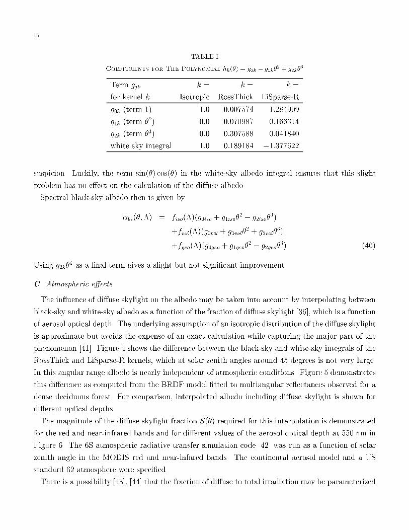
TABLE I
Coefficients for The Polynomial hk(�) = g0k + g1k�2 + g2k�
3
Term gjk k = k = k =
for kernel k Isotropic RossThick LiSparse-R
g0k (term 1) 1:0 �0:007574 �1:284909
g1k (term �2) 0:0 �0:070987 �0:166314
g2k (term �3) 0:0 0:307588 0:041840
white-sky integral 1:0 0:189184 �1:377622
suspicion. Luckily, the term sin(�) cos(�) in the white-sky albedo integral ensures that this slight
problem has no e�ect on the calculation of the di�use albedo.
Spectral black-sky albedo then is given by
�bs(�;�) = fiso(�)(g0iso + g1iso�2 + g2iso�
3)
+fvol(�)(g0vol + g1vol�2 + g2vol�
3)
+fgeo(�)(g0geo + g1geo�2 + g2geo�
3) (46)
Using g2k�4 as a �nal term gives a slight but not signi�cant improvement.
C. Atmospheric e�ects
The in uence of di�use skylight on the albedo may be taken into account by interpolating between
black-sky and white-sky albedo as a function of the fraction of di�use skylight [36], which is a function
of aerosol optical depth. The underlying assumption of an isotropic distribution of the di�use skylight
is approximate but avoids the expense of an exact calculation while capturing the major part of the
phenomenon [41]. Figure 4 shows the di�erence between the black-sky and white-sky integrals of the
RossThick and LiSparse-R kernels, which at solar zenith angles around 45 degrees is not very large.
In this angular range albedo is nearly independent of atmospheric conditions. Figure 5 demonstrates
this di�erence as computed from the BRDF model �tted to multiangular re ectances observed for a
dense deciduous forest. For comparison, interpolated albedo including di�use skylight is shown for
di�erent optical depths.
The magnitude of the di�use skylight fraction S(�) required for this interpolation is demonstrated
for the red and near-infrared bands and for di�erent values of the aerosol optical depth at 550 nm in
Figure 6. The 6S atmospheric radiative transfer simulation code [42] was run as a function of solar
zenith angle in the MODIS red and near-infared bands. The continental aerosol model and a US
standard 62 atmosphere were speci�ed.
There is a possibility [43], [44] that the fraction of di�use to total irradiation may be parameterized

17
in a relatively simple way at least for moderate solar zenith angles by assuming a linear relationship
between S(�) and �(�). The slope and intercept are determined from simulation or observation as a
simple function of wavelength (see [43]). �(�) itself is parameterized as a power function of the wave-
length with the exponent empirically or theoretically determined (� 1:3) and the scaling factor of the
power function the only remaining variable, characterizing turbidity. This approach seems to be rela-
tively reliable in the visible domain, which is the domain contributing most to broadband albedo and
could lead to a further simpli�cation of the current algorithm through additional parameterization.
D. Spectral-to-Broadband Albedo Conversion
Spectral-to-broadband conversion is based on the sparse angular sampling that satellite sensors like
MODIS, MISR, POLDER, MERIS or the AVHRR provide. The MODIS sensor has seven discrete
shortwave bands, three in the visible and four in the infrared [45]. MISR also provides three visible
bands but has only one band in the near-infrared [46]. MERIS has programmable bands in the visible
and near-infrared. The AVHRR sensor provides only the red band for estimation of the visible and
the near-infrared band for estimation of the near-infared broadband albedo [47].
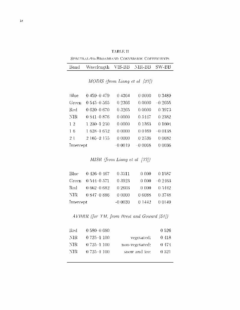
Various studies in the published literature suggest spectral-to-broadband conversion coe�cients
which allow to estimate broadband albedos from such spectrally sparse observations. Liang et al.
[37] used observed spectra and numerical simulations to produce conversion coe�cients for MODIS
and MISR. Several authors provide conversion coe�cients for the AVHRR (e.g., [48]{[50]). Of these,
we found the coe�cients given by Brest and Goward [51] to be reliable even though they were derived
for working with Landsat TM data. Coe�cients are listed in Table II.
One should keep in mind that spectral-to-broadband conversion is a function of atmospheric state
to the extent that the spectral distribution of the solar downwelling ux depends on atmospheric
properties and the solar zenith angle. The conversion coe�cients listed in Table II are derived for
typical average cases. Variations of the exact results with aerosol optical depth and solar zenith angle
are small but a�ect retrieval accuracies on the level of a few percent.
VI. ALGORITHM VALIDATION
A. Ross-Li BRDF Model Validation
A basic requirement of the BRDF model to be used is that it is capable of representing accurately
the shapes of naturally occurring BRDFs. Earlier work using various forms of kernel-based models
already has demonstrated the feasibility of this approach in BRDF modeling [32], [52] [53]. These
works show that kernel-based models give reasonable �ts to �eld-measured BRDF data sets in the
sense that they reproduce with their three parameters all the major features of the BRDF for a wide
variety of situations including barren and densely vegetated cases.
In order to speci�cally study the Ross-Li model proposed here, a set of 61 very diverse �eld-measured
18
TABLE II
Spectral-to-Broadband Conversion Coefficients
Band Wavelength VIS-BB NIR-BB SW-BB
MODIS (from Liang et al. [37])
Blue 0.459{0.479 0.4364 0.0000 0.3489
Green 0.545{0.565 0.2366 0.0000 {0.2655
Red 0.620{0.670 0.3265 0.0000 0.3973
NIR 0.841{0.876 0.0000 0.5447 0.2382
1.2 1.230{1.250 0.0000 0.1363 0.1604
1.6 1.628{1.652 0.0000 0.0469 {0.0138
2.1 2.105{2.155 0.0000 0.2536 0.0682
Intercept {0.0019 {0.0068 0.0036
MISR (from Liang et al. [37])
Blue 0.426{0.467 0.3511 0.000 0.1587
Green 0.544{0.571 0.3923 0.000 {0.2463
Red 0.662{0.682 0.2603 0.000 0.5442
NIR 0.847{0.886 0.0000 0.6088 0.3748
Intercept -0.0030 0.1442 0.0149
AVHRR (for TM, from Brest and Goward [51])
Red 0.580{0.680 0.526
NIR 0.725{1.100 vegetated: 0.418
NIR 0.725{1.100 non-vegetated: 0.474
NIR 0.725{1.100 snow and ice: 0.321
19
BRDF data sets was assembled. These cover all major types of landcover, such as dense and sparse
broadleaf and grasslike crops of various types on bright and dark soils, needleleaf and broadleaf forests
including situations with snow backgrounds and barren trees, tundra, desert, snow, dark and bright
barren soils etc. Most of these data sets were acquired using the PARABOLA instrument by Deering
and coworkers [54]{[56], but others are included as well. These latter datasets are mostly ground-
based observations as well, for example those by Kimes and coworkers [57]{[59] but also include some
acquired from the air. The total of 61 datasets may not be completely representative in terms of
the distribution of types but gives an indication of model performance based on the current state
of BRDF �eld observation. Most sets have excellent coverage of the viewing hemisphere at several
di�erent solar zenith angles. Only a few sets are sparse.
Each of the 61 data sets was inverted using the Ross-Li BRDF model. The residual deviation
between modeled and observed re ectances, the RMSE, was expressed as a fraction of the typical
re ectance, here represented by the white-sky albedo as predicted by the model. The average RMSE
was 20 percent of the white-sky albedo in the red and 15 percent in the near-infrared band. The
median values were 16 and 13 percent, respectively. These errors include artifacts and inconsistencies
in the �eld data. For example, some data sets as measured display an irregular variability of the
re ectance at some angles that may be due to the di�culty of the measurement. This variability will
naturally contribute to the RMSE found in inversion.
The results found for the Ross-Li model are almost identical to those for other well-established
semiempirical BRDF models. The non-reciprocal original RossThick-LiSparse BRDF model [33], the
RossThick-Roujean model [32], the modi�ed Walthall model [19], [38] and the modi�ed Rahman
model [60] all have red band average RMSEs of between 19 and 21 percent of the white-sky albedo
(14 to 18 percent in the median), and average near-infrared band RMSEs between 14 and 16 percent
of the white-sky albedo (11 to 14 percent in the median).
Histograms of the RMSE look very similar for all of the models. Figure 7 shows the accumulative
percentage of datasets with RMSEs below a given threshold. All �ve semiempirical BRDF models
studied, which all use three parameters to model the BRDF, show a very similar behavior. Where
one model has di�culties representing the observed BRDF in all its complexity, others generally have
the same problem. This may be due to similar de�ciencies of each model or pecularities in the �eld
data.
The RMSEs found are not all as small as one would like, but to the extent that a simple three-
parameter general inversion model can be expected to model the complexities of a great variety of
BRDF datasets acquired in the �eld they are satisfactory. Visual inspection of re ectance plots
shows that the basic multidirectional anisotropy of very di�erent land surfaces may be adequately
modeled, even though details like the behavior at large zenith angles or in the hotspot region may
be represented less accurately. Improved models with a relative RMSE below 10 percent in all cases
20
would be much desired in the near future.
Even though the models are very similar in their ability to �t �eld-observed BRDFs when well
constrained by observations, they display di�erent capabilities to predict the BRDF and albedo from
sparse angular sampling or noisy data. For example, the empirical modi�ed Walthall model is less
reliable in this respect due to its lack of a semiphysical basis [61]. For the Ross-Li BRDF model these
issues are addressed in the following section.
B. Inversion Accuracy with Sparse Angular Sampling
Even if a BRDF model is able to represent land surface BRDFs su�ciently well under conditions
of good angular sampling, it is important to investigate whether the retrievals remain stable when
angular sampling is sparse, as is the case from space-based satellite sensors. The achievable accuracy
will depend not only on the number of observations but also on their angular distribution, that is,
on sensor scan pattern and orbit, latitude and solar zenith angle.
Re ectance and albedo retrieval accuracies under sparse angular sampling were investigated for
kernel-driven models by Privette et al. [62] and Lucht [61]. The former paper relied on �eld-observed
BRDFs that were systematically sampled sparsely. Ten di�erent simple BRDF models were tested.
The latter paper used a discrete ordinates radiative transfer code by Myneni et al. [63] to generate
synthetic re ectances for the exact MODIS and MISR observation geometries throughout the year.
The �rst study [62] did not include the Ross-Li BRDF model but used its non-reciprocal version,
which is very similar at most angles. It concluded that this model was one of two models that
performed best overall. The second study [61] did use the Ross-Li model. The detailed results
found for albedo and re ectance inversion accuracies are summarized in Table III. The �rst is for
cloudfree conditions, indicating the achievable accuracies under optimal sampling conditions. The
second investigates the accuracies found when half of the observations are lost due to clouds. This
last condition does not apply to the MISR instrument, which acquires the multiangular observations
instantaneously and therefore generally provides either all views or none.
The analysis was carried out for MODIS and for MISR angular sampling as well as for combined
sampling for six di�erent surface types, the red and the near-infrared bands, observations geometries
throughout the year and at di�erent latitudes from pole to pole. The sampling period was 16 days.
Median accuracies and ranges encompassing two thirds of all values are listed for retrievals of black-
sky albedo at the respective mean solar zenith angle of the observations (which varies with latitude
and time of year) and for other solar zenith angles (i.e., 0, 30 and 60 degrees, and for the white-sky
albedo, irrespective of the solar zenith angle of observation). The latter poses a very severe test,
as albedo is retrieved at solar zenith angles that are potentially far from the angles sampled. For
example, at high latitudes the solar zenith angle of the observations may have been 70 degrees, but
the accuracy of correctly predicting albedo is also investigated for a nadir solar zenith angle. Even

21
though the sun will never be at nadir at the extreme latitude of this example, the re ective properties
of the surface at such angles still play a role under di�use illumination conditions, for example an
overcast sky.
Table III reveals that retrievals generally achieve accuracies within 10 percent in the red band
with a median error of around 5 percent. These percentages are relative to the true albedo. In the
near-infrared band, retrievals are accurate to within 5 percent, with a median of about 3 percent.
Cloudiness does not severely a�ect the retrieval accuracy of combined MODIS and MISR sampling
as long as the angular distribution of the samples lost to clouds is relatively random. Cloudiness
increases errors by several percent if only MODIS angular sampling is used.
At solar zenith angles extrapolated freely away from that of the observation the errors are somewhat
larger, as expected. Median errors in the red band are around 8 percent, with worst cases producing
errors of up to 20 percent. In the near-infrared band, the median error is about 4 percent, also with
20 percent errors possible in the worst cases. Given the angular sampling available from the sensors,
and the very severe test these extrapolations pose, these are very satisfactory results. In a typical
case, albedo at any solar zenith angle will be retrieved to within 10 percent relative. This accuracy
should be a great improvement over other techniques for determining albedo which do not explicitly
take into account the bidirectional e�ects of the surface.
The accuracy found for angular sampling provided by MODIS alone should be comparable to that
provided by AVHRR or by MERIS. The combined sampling of MODIS and MISR is not quite as good
as that achieved by POLDER over several orbits. The paper by Lucht [61] gives more detailed results
and also investigates the accuracy with which BRDF-corrected nadir re ectance, of importance for
BRDF-normalization of images or vegetation indices, is retrieved at di�erent solar zenith angles.
C. Noise Sensitivity
When multiangular observations from di�erent orbits are assembled over a period of time to provide
a varied angular sampling for BRDF model inversion, as is required for observations from MODIS,
MERIS or the AVHRR, a certain amount of noise-like variation may be expected in the data. This
is due to slight changes in surface moisture, atmospheric conditions, geolocation, footprint size etc.
from one orbit to the next.
The sensitivity to noise of re ectance and albedo retrieval using the nonreciprocal RossThick-
LiSparse kernel-driven BRDF models was investigated systematically by Lucht and Lewis [64]. Re-
sults were found to be very similar for di�erent kernel-based models so that they are also relevant for
the reciprocal Ross-Li BRDF model. So-called weights of determinations, or noise sensitivity factors,
are derived analytically from an analysis of the matrix inverting the kernel-driven BRDF model (see
equation 24). These factors specify the level of noise expected in a given computed linear function of
the model parameters (such as the model parameters, re ectance or albedo) as a fraction of the noise

22
TABLE III
Albedo Retrieval Accuracies (Median and Range, Percent Relative) (after Lucht [61]; expanded).
Sensor(s), Cloudiness Red Band NIR Band
At solar zenith angle of observations
MODIS 0% 5.5 (2.7{10.6) 3.5 (1.4{5.3)
MISR 0% 4.1 (2.1{10.7) 2.4 (1.0{5.5)
MODIS+MISR 0% 4.4 (0.7{10.1) 2.0 (0.8{4.9)
MODIS 50% 7.7 (1.6{13.0) 4.5 (0.7{8.1)
MISR 50% n/a n/a
MODIS+MISR 50% 4.1 (1.6{10.1) 2.3 (0.7{5.4)
At other solar zenith angles
MODIS 0% 7.6 (1.9{19.6) 3.5 (1.2{19.0)
MISR 0% 5.6 (1.3{19.2) 3.0 (0.9{12.0)
MODIS+MISR 0% 5.5 (1.3{18.4) 2.4 (0.8{13.1)
MODIS 50% 9.5 (2.3{22.2) 6.7 (0.9{19.5)
MISR 50% n/a n/a
MODIS+MISR 50% 5.7 (1.6{18.6) 4.5 (0.8{13.9)
in the observed re ectances, which is estimated to be equal to the RMSE. Values less than unity
indicate a suppression of noise in the retrieval, factors larger than unity an increase. Noise sensitivity
factors are independent of wavelength due to the mathematical form of kernel-based models as long
as the weights wl used in the inversion are not wavelength-dependent. They depend on the exact
location of the angular sampling acquired.
Table IV summarizes noise sensitivities for di�erent sensors and fractions of observations lost due
to clouds. Again the cloudy case is not relevant for MISR as this instrument either acquires all
observations in a short period of time over cloud-free skies or none at all. The time period used for
MODIS is 16 days, and that for MISR 9 days, which are the respective periods used for producing
the operational albedo products for each sensor. Clearly, all the retrievals at the mean solar zenith
angle of the observations are stable against noise. If the inputs had a random component of, for
example, 10 percent magnitude, the albedos retrieved would only vary by about 2 to 5 percent. The
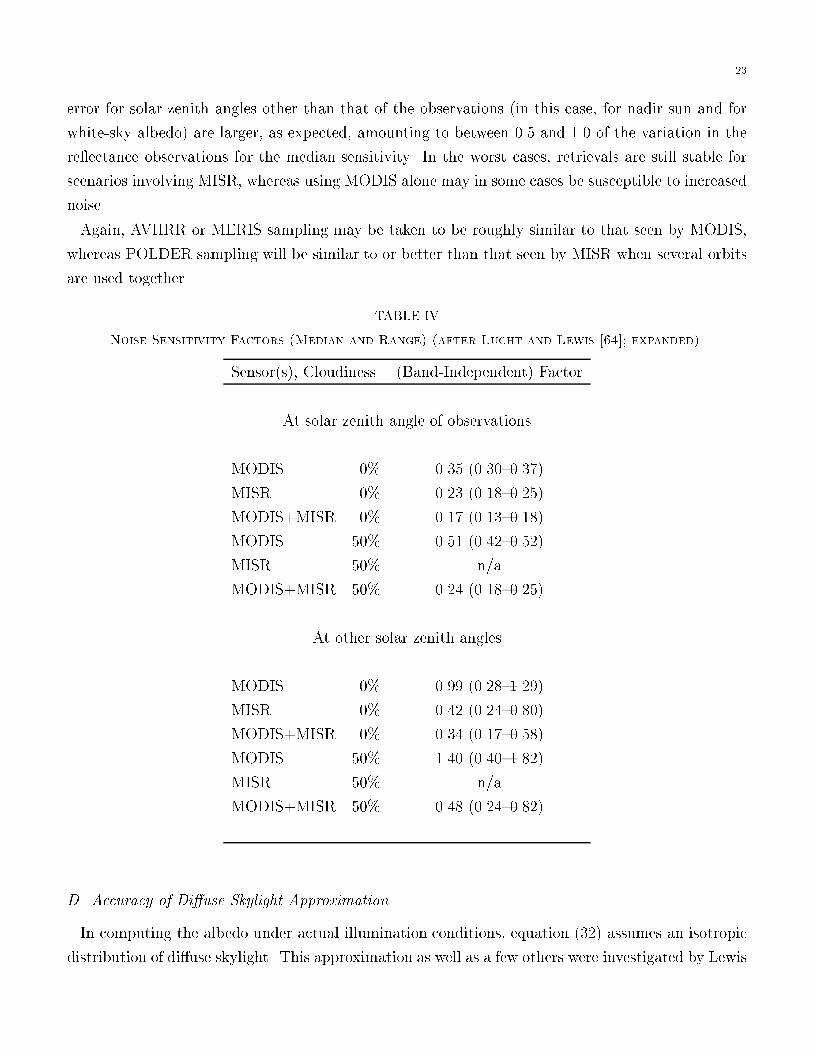
23
error for solar zenith angles other than that of the observations (in this case, for nadir sun and for
white-sky albedo) are larger, as expected, amounting to between 0.5 and 1.0 of the variation in the
re ectance observations for the median sensitivity. In the worst cases, retrievals are still stable for
scenarios involving MISR, whereas using MODIS alone may in some cases be susceptible to increased
noise.
Again, AVHRR or MERIS sampling may be taken to be roughly similar to that seen by MODIS,
whereas POLDER sampling will be similar to or better than that seen by MISR when several orbits
are used together.
TABLE IV
Noise Sensitivity Factors (Median and Range) (after Lucht and Lewis [64]; expanded).
Sensor(s), Cloudiness (Band-Independent) Factor
At solar zenith angle of observations
MODIS 0% 0.35 (0.30{0.37)
MISR 0% 0.23 (0.18{0.25)
MODIS+MISR 0% 0.17 (0.13{0.18)
MODIS 50% 0.51 (0.42{0.52)
MISR 50% n/a
MODIS+MISR 50% 0.24 (0.18{0.25)
At other solar zenith angles
MODIS 0% 0.99 (0.28{1.29)
MISR 0% 0.42 (0.24{0.80)
MODIS+MISR 0% 0.34 (0.17{0.58)
MODIS 50% 1.40 (0.40{1.82)
MISR 50% n/a
MODIS+MISR 50% 0.48 (0.24{0.82)
D. Accuracy of Di�use Skylight Approximation
In computing the albedo under actual illumination conditions, equation (32) assumes an isotropic
distribution of di�use skylight. This approximation as well as a few others were investigated by Lewis

24
TABLE V
Average Relative Broadband Albedo Prediction Error and Best-Worst Range From Using
Narrow-to-Broadband Coefficients
Band MODIS MISR AVHRR
SW-BB 6% (1{10%) 6% (1{13%) 4% (0{7%)
VIS-BB 4% (0{11%) 5% (3{10%) |
NIR-BB 3% (1{5%) 13% (10{21%) |
and Barnsley [36]. They �nd that the approximation is very good, with relative errors generally less
than a few percent even in the worst cases, which occur for small solar zenith angles.
E. Accuracy of Spectral-to-Broadband Conversion
Six representative spectra taken from the ASTER spectral library were used to investigate spectral-
to-broadband conversion. These are three spectra for vegetation (deciduous tree leaves, conifer tree
needles, green grass) and three for barren surfaces (brown silty loam, dark reddish brown �ne sandy
loam, �ne snow). Taking these re ectance spectra as an estimate of albedo spectra, which should
have very similar properties, exact broadband albedos in the total shortwave (0.3 to 5.0 �m), visible
(0.3 to 0.7 �m) and near-infrared (0.7 to 5.0 �m) broadbands were computed by convolving with the
downwelling solar spectrum. The latter was computed using the 6S code [42], the sun at nadir, a
continental aerosol model and a US standard 62 atmosphere.
Figure 8 shows the spectra studied and plots the exact broadband albedos for comparison with
the values estimated from discrete albedos in satellite spectral bands, the latter derived using the
conversion coe�cients of Table II. Even though vegetation, soils and snow have rather di�erent
spectra, results from the MODIS bands are correct to within 10 percent relative for all surface types
and all three broadbands. The mean relative error for the total shortwave, visible and near-infrared
broadband albedo is 6, 4 and 3 percent, respectively.
The corresponding errors when using only the four MISR bands are 6, 5 and 13 percent (Table V).
As expected, the near-infared broadband albedo can be predicted with considerably less reliability
from MISR than from MODIS. The error is up to 20 percent in individual cases. However, this does
not strongly impact the accuracy of the total shortwave broadband albedo from MISR due to the
small contribution of the solar downwelling ux in the near-infared.
While some published conversion coe�cients for the AVHRR red and near-infrared bands produced
errors of 15 to 60 percent relative, it was surprising that the coe�cients given by Brest and Goward

25
[51] for Landsat TM spectral bands produced very good results for the six very di�erent spectra used
here and for the corresponding AVHRR bands. The mean error of the total shortwave broadband
albedo was only 4 percent, all estimated albedos being slightly too small. This is excellent given that
the spectral sampling for the AVHRR is as sparse as is possible. If con�rmed for a larger number of
spectra, this bodes well for deriving broadband albedo from the long data record available only from
the AVHRR. Also, the conversion coe�cients for vegetated surfaces were used throughout. When
using the non-vegetated coe�cients for the barren surfaces, the results are worse. When using the
snow coe�cients for the snow case, the result improves.
Required broadband albedo accuracies for climate modeling purposes of 0.05 [22] or 0.02 [9], [27]
are frequently cited. Since the total shortwave broadband albedo of vegetation is about 0.25 and
that of moderately bright soils about 0.35, an error of 6 percent relative in this albedo would provide
an accuracy of about 0.02 and hence meet the requirements, although inversion accuracy and noise
sensitivity errors will add to this error in the �nal analysis.
Since spectral-to-broadband conversion is dependent on the spectral distribution of the solar down-
welling ux and therefore on atmospheric state, the conversion coe�cients listed in Table II are
derived for typical or average cases.
F. Albedo Field Validation
A validation study investigating the derivation of broadband albedos from AVHRR and POLDER
multiangular observations was carried out at a semidesert site in May 1997 in Jornada, New Mexico
as part of the MODIS land prototyping exercise PROVE '97 [65]. Total shortwave and near-infrared
broadband albedos were measured on the ground using upward and downward-looking pyranometers.
Visible broadband albedos were inferred mathematically from these measurements.
Data were collected at 44 locations along four 100 m transects radiating away from a tower in a
soil-dominated landscape featuring scattered mesquite and yucca bushes and patches of dry senes-
cent grass. Some measurements were also made at a location dominated by the senescent grass.
The broadband albedo of the tower site was taken to be well represented by the average of these
measurements. Furthermore, the albedo of a square kilometer surrounding the tower was determined
by coarsely classifying the area from high-resolution aircraft-acquired imagery and assigning typical
albedos to scene components based on �ndings from the ground observations [65].
Albedos were also derived from the atmospherically corrected multiangular observations acquired
by the AVHRR on NOAA-14 and by POLDER during the time period of the �eld measurements.
The Ross-Li BRDF model was inverted to obtain black-sky and white-sky albedo in the red and near-
infrared spectral bands. Concurrent AVIRIS spectra were then used to qualitatively extrapolate these
measurements over the full spectral range to derive broadband albedos. The AVHRR observations
were modeled for the 1.1-km pixel containing the tower, for a block of 2 by 2 pixels, and for an area

26
TABLE VI
Comparison of Field-Observed Total Shortwave Broadband Albedos with Satellite-Derived
Values at Jornada, New Mexico (using data by Hyman et al. [65]).
Band Observed Relative Di�erence
Value AVHRR POLDER
SW-BB 0.221 2% 1%
VIS-BB 0.124 3% 7%
NIR-BB 0.311 1% 3%
of 10 by 10 pixels covering the region. The POLDER pixel modeled has a resolution of about 7 km.
Albedos were corrected for di�use skylight using the interpolation method given in this paper. The
paper by Hyman et al. [65] provides details.
Table VI lists the relative deviation between the ground measurements, the albedos derived from the
1-km AVHRR processing, and those derived from POLDER. The broadband albedos from the space-
based sensors are in excellent agreement with those observed on the ground in all three broadbands.
Only the visible broadband as deduced from POLDER is not in complete agreement with the ground
observations, but the spatial scale of the POLDER observations is much larger than the spatial
extent of the ground measurements, and the landscape shows some variability on the scale of several
hundred meters.
Figure 9 graphically compares the results found with the range of possible albedos at the site
represented by the scene component albedos, and with the potential albedo of an arbitrary unknown
pixel. Clearly, space-based retrieval of broadband albedos from sparse spectral observations following
the algorithm given here worked very well for this site.
Albedo validation using airborne multiangle imagery was performed by Lewis et al. [66] for a
semiarid area in Niger. Data acquired by ASAS were inverted using kernel-driven BRDF models.
Broadband albedos were derived from spectral albedos in four bands and coupling with the prevailing
atmosphere. Comparison with ground measurements over a millet canopy and for a soil/tiger bush
site showed an excellent correlation coe�cient of 0.98. On the basis of this validation, spatial maps
of albedo were derived for a larger area, demonstrating the algorithm outlined here on airborne data.
27
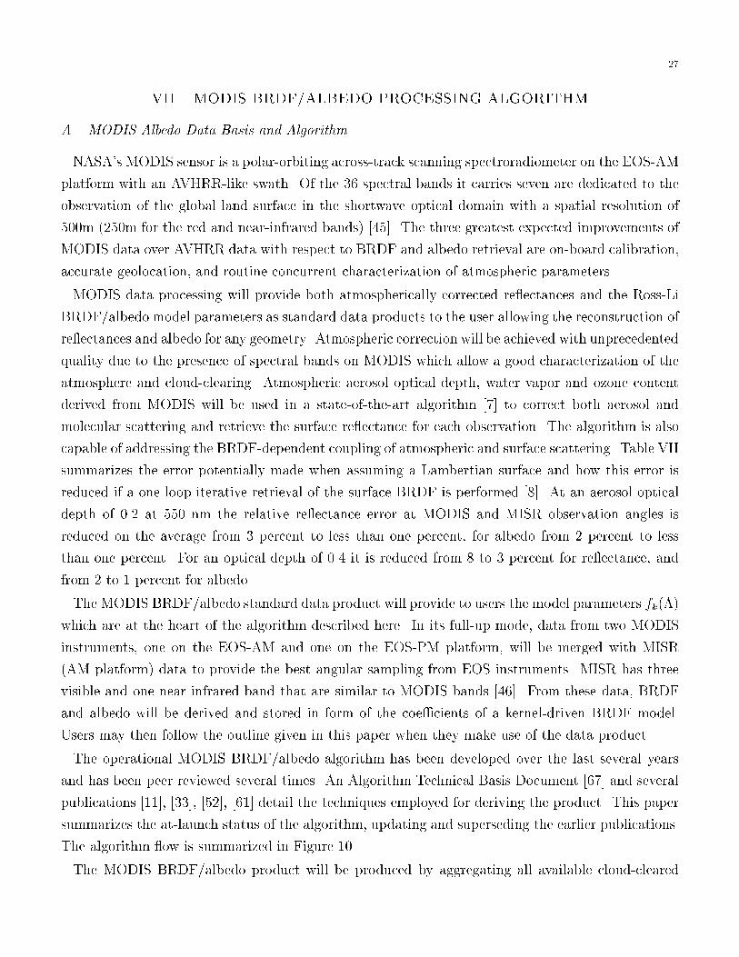
VII. MODIS BRDF/ALBEDO PROCESSING ALGORITHM
A. MODIS Albedo Data Basis and Algorithm
NASA's MODIS sensor is a polar-orbiting across-track scanning spectroradiometer on the EOS-AM
platform with an AVHRR-like swath. Of the 36 spectral bands it carries seven are dedicated to the
observation of the global land surface in the shortwave optical domain with a spatial resolution of
500m (250m for the red and near-infrared bands) [45]. The three greatest expected improvements of
MODIS data over AVHRR data with respect to BRDF and albedo retrieval are on-board calibration,
accurate geolocation, and routine concurrent characterization of atmospheric parameters.
MODIS data processing will provide both atmospherically corrected re ectances and the Ross-Li
BRDF/albedo model parameters as standard data products to the user allowing the reconstruction of
re ectances and albedo for any geometry. Atmospheric correction will be achieved with unprecedented
quality due to the presence of spectral bands on MODIS which allow a good characterization of the
atmosphere and cloud-clearing. Atmospheric aerosol optical depth, water vapor and ozone content
derived from MODIS will be used in a state-of-the-art algorithm [7] to correct both aerosol and
molecular scattering and retrieve the surface re ectance for each observation. The algorithm is also
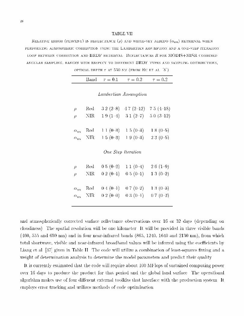
capable of addressing the BRDF-dependent coupling of atmospheric and surface scattering. Table VII
summarizes the error potentially made when assuming a Lambertian surface and how this error is
reduced if a one-loop iterative retrieval of the surface BRDF is performed [8]. At an aerosol optical
depth of 0.2 at 550 nm the relative re ectance error at MODIS and MISR observation angles is
reduced on the average from 3 percent to less than one percent, for albedo from 2 percent to less
than one percent. For an optical depth of 0.4 it is reduced from 8 to 3 percent for re ectance, and
from 2 to 1 percent for albedo.
The MODIS BRDF/albedo standard data product will provide to users the model parameters fk(�)
which are at the heart of the algorithm described here. In its full-up mode, data from two MODIS
instruments, one on the EOS-AM and one on the EOS-PM platform, will be merged with MISR
(AM platform) data to provide the best angular sampling from EOS instruments. MISR has three
visible and one near-infrared band that are similar to MODIS bands [46]. From these data, BRDF
and albedo will be derived and stored in form of the coe�cients of a kernel-driven BRDF model.
Users may then follow the outline given in this paper when they make use of the data product.
The operational MODIS BRDF/albedo algorithm has been developed over the last several years
and has been peer reviewed several times. An Algorithm Technical Basis Document [67] and several
publications [11], [33], [52], [61] detail the techniques employed for deriving the product. This paper
summarizes the at-launch status of the algorithm, updating and superseding the earlier publications.
The algorithm ow is summarized in Figure 10.
The MODIS BRDF/albedo product will be produced by aggregating all available cloud-cleared
28
TABLE VII
Relative error (percent) in reflectance (�) and white-sky albedo (�ws) retrieval when
performing atmospheric correction using the Lambertian assumption and a one-step iteration
loop between correction and BRDF retrieval. Reflectances R for MODIS+MISR combined
angular sampling, ranges with respect to different BRDF types and sampling distributions,
optical depth � at 550 nm (from Hu et al. [8]).
Band � = 0:1 � = 0:2 � = 0:2
Lambertian Assumption
� Red 3.2 (2{8) 4.7 (2{12) 7.5 (4{18)
� NIR 1.9 (1{4) 3.1 (2{7) 5.0 (3{12)
�ws Red 1.1 (0{3) 1.5 (0{3) 1.8 (0{5)
�ws NIR 1.5 (0{3) 1.9 (0{3) 2.3 (0{5)
One-Step Iteration
� Red 0.5 (0{2) 1.1 (0{4) 2.6 (1{9)
� NIR 0.2 (0{1) 0.5 (0{1) 1.3 (0{2)
�ws Red 0.4 (0{1) 0.7 (0{2) 1.3 (0{3)
�ws NIR 0.2 (0{0) 0.3 (0{1) 0.7 (0{2)
and atmospherically corrected surface re ectance observations over 16 or 32 days (depending on
cloudiness). The spatial resolution will be one kilometer. It will be provided in three visible bands
(460, 555 and 659 nm) and in four near-infrared bands (865, 1240, 1640 and 2130 nm), from which
total shortwave, visible and near-infrared broadband values will be inferred using the coe�cients by
Liang et al. [37] given in Table II. The code will utilize a combination of least-squares �tting and a
weight of determination analysis to determine the model parameters and predict their quality.
It is currently estimated that the code will require about 100 MFlops of sustained computing power
over 16 days to produce the product for that period and the global land surface. The operational
algorithm makes use of four di�erent external toolkits that interface with the production system. It
employs error tracking and utilizes methods of code optimization.

29
B. MODIS BRDF/Albedo Product
The MODIS BRDF/albedo standard data product (called MOD43) will be subdivided into four
di�erent components, two full BRDF/albedo products and two ready-to-use utility products:
1. The semiempirical Ambrals BRDF/albedo product. This product will supply coe�cients for
the Ross-Li semiempirical BRDF/albedo model for each global 1km land pixel in the seven
MODIS land bands and the visible, near-infrared and total shortwave broadbands. A full array
of per-band quality control information as well as shape factors that give forward-to-nadir and
backward-to-nadir modeled re ectance ratios for 30� viewing and 45� solar zenith angle are also
carried. The code is capable of running di�erent kernel-driven BRDF models in competition [11],
but this feature will not initially be used.
2. The empirical modi�ed Walthall BRDF/albedo product. This product is structurally the same
as the semiempirical BRDF/albedo product but is based on the empirical modi�ed Walthall
BRDF model, which provides a very simple one-line parameterization of multiangular re ectance
and is also of the kernel-driven type [19], [38]. Depending on the frequency of user requests this
product may in the future be upgraded to a next generation of BRDF models under development
while the semiempirical product is continued for time series consistency.
3. The minimal albedo product. Since the BRDF/albedo products which carry the full BRDF/albe-
do information tend to be rather large and contain albedo in a parameterized form, an easy-to-use
smaller-volume albedo product is generated which carries only a subset of the complete albedo
and no BRDF information. Black-sky albedo for 45� solar zenith and white-sky albedo are given
in 4 bands (460, 659, 865, 1640 nm) and the visible and NIR broadbands.
4. The BRDF-corrected nadir re ectance product. This product will provide a nadir-view re-
ectance in all seven bands derived from the semiempirical BRDF modeling product at the
median solar zenith angle of observation. Nadir-view nadir-sun re ectance is one of the model
parameters in the semiempirical BRDF/albedo product.
File sizes for the four products will be 0.75, 0.93, 0.28 and 0.21 Gigabytes per day for all global land
pixels, or 11.7, 14.9, 4.5 and 3.3 Gigabytes per full 16-day or 32-day product. Each product will be
available in tiles that measure 1200 by 1200 one kilometer pixels which are subsets of the integerized
sinusoidal grid that is being used as the geographical storage format [68]. All products will be in the
HDF format with an EOS enhancement that allows geographical subsetting (HDF-EOS).
C. Albedo Derivation From Very Sparse Angular Sampling
Realistically, the number of available multiangular observations and their angular range are at
times insu�cient for a reliable BRDF inversion and albedo derivation. The main reasons for this are
loss of observations to cloud cover, orbital constraints, and the limited length of time for which data
should reasonably be aggregated. In fact, where data of the type produced by MODIS or AVHRR

30
are used as the sole data source and are aggregated for 2 to 4 weeks, between a third and one half of
global pixels are likely a�ected by insu�cient angular sampling [69], [70]. In some regions, as in the
tropics, persistent cloud cover will make good angular sampling an occasional event. The weights
of determination can be utilized to identify pixels with insu�ent angular sampling to con�dently
perform a BRDF inversion.
Therefore, a back-up algorithm is employed for deriving albedo in a situation of insu�cient angular
sampling. This algorithm should make full use of the sparse multiangular information that is available.
The approach being followed is to constrain the BRDF shape from prior information but to adjust it
to match the observations made. If an estimate of the BRDF shape is available in the form of BRDF
model parameters f 0
k, then an estimate of the new observed BRDF may be obtained by �nding the
factor q that minimizes
e02 =Xl
f�(�l; #l; �l)� q R0(�l; #l; �l)g2
(47)
=Xl
(�(�l; #l; �l)� q
Xk
f 0
kKk(�l; #l; �l)
);
where �l are the observed and R0
l the re ectances estimated from the a priori BRDF model. Mini-
mizing this equation leads to the observation-adjusted new model parameters
fk = q f 0
k =
Pl �(�l; #l; �l)R
0(�l; #l; �l)PlR0(�l; #l; �l)2
f 0
k; (48)
where the value of q should generally not be substantially di�erent from unity.
The basis of this derivation is the assumption that the shape of a given BRDF type approximately
scales linearly with the overall re ectance at least over part of the possible re ectance range. In other
words, the shape of a BRDF will be linearly more pronounced or less pronounced in proportion to
the overall re ectance of the scene. This assumptions is certainly not generally valid but will capture
a large portion of the e�ect that is to be modeled. Generally, a dark scene with a low contrast
between scene elements will show a relatively weak BRDF, whereas a scene with a stronger contrast
between scene elements due to one scene component possessing a larger component signature will
produce a stronger shape. As scene properties are assumed to be the same otherwise, the shape
of the BRDFs will be similar in a relative sense to the extent that the physics of scattering will
not be substantially changed by the di�erence in brightness. In reality, brighter scenes will lead
to more multiple scattering among other e�ects, but this will usually not be a dominant in uence.
Some evidence of shape similarity may be seen in Figure 5, where the solar zenith-angle dependence
of a deciduous forest is similar in the red and the near-infrared wavebands in a relative manner,
the absolute scales being di�erent in each case. However, this procedure is meant to model small
variations in surface brightness from one case to the other, not di�erences as large as the di�erence
31
between, e.g., red and near-infrared BRDFs. A di�erent estimated BRDF f 0
k should be used in this
case for each band to be modeled. Most importantly, the estimated BRDF will be scene-dependent,
for example land cover dependent.
If only one observation is used, for example because the data basis is maximum-value composited,
these relationships are reduced to
fk = q f 0
k =�(�; #; �)
R0(�; #; �)f 0
k; (49)
that is the parameters, and hence the re ectances and the albedos as well, are simply scaled by the
ratio of observed and a priori BRDF model-estimated re ectance at the viewing and illumination
geometry of the single observation used [14], [71]. Naturally, using just one observation will be less
reliable than using several observations but should still coarsely adjust the BRDF and the albedo to
local pixel properties.
In cases where the number of observations available is too small for a full BRDF inversion, the
MODIS BRDF product will utilize a global BRDF database to predict a shape type for the BRDF,
which will then be adapted to �t the available observations following the procedure given. The
heritage of the data given is agged in each case. The BRDF database will initially be a land
cover-derived database where the BRDFs used are �eld-observed BRDFs adjusted to re ect AVHRR
re ectances for each location and season [71]. In the post-launch period the database will be itera-
tively repopulated by MODIS-derived BRDFs.
D. BRDF Model Alternatives
From the above discussions the advantages of using a kernel-based BRDF model should be obvious.
A potential not yet realized is that the full and very well developed apparatus of the theory of linear
systems could be brought to bear onto analyzing the BRDF inversion process with linear models.
Advanced treatments are readily available, for example [72]{[74].
In this paper, the Ross-Li BRDF model was the focus. Alternative kernel-based BRDF models are
available. Roujean et al. [32] provide a geometric-optical kernel based on rectangular protrusions.
This model is being employed by the POLDER project [10]. Chen and Cihlar [75] have expanded this
model to include a more prominent hotspot formulation, at the cost of introducing two additional
nonlinear parameters that require pre-determination in the framework of a linear modeling concept.
Wanner et al. [33] give formulations for alternate volumetric and geometric kernels making di�erent
assumptions about the canopy modeled. These are less general than the RossThick-LiSparse-R
combination but may be more appropriate for certain types of scenes [52].
The modi�ed Walthall model [19], [38] is a fully empirical kernel-based model. It is interesting
because of its one-line mathematical simplicity but has been shown to be less accurate in angular
32
extrapolation under conditions of sparse angular sampling [61]. This is not surprising given the
straight-forward geometric nature of the empirical terms employed.
However, BRDF models that are not kernel-based are also available. Of these, mainly the three-
parameter models are of interest here as it is doubtful that more than three parameters can be reliably
retrieved from space-based remote sensing. The most important of these is the model employed for
the MISR albedo product, a modi�ed version [12] of a semiempirical three-parameter model by
Rahman et al. [60]. This model is only semilinear in its modi�ed form and is nonlinear in its original
form, which according to Privette et al. [62] is the superior form. Several studies [52], [61], [64] have
concluded that the modi�ed Rahman model is very comparable to the Ross-Li BRDF model used
here, showing similar trends in �tting as well as similar problems. In practical applications, and
under sparse angular sampling, the Rahman model may be somewhat more sensitive to changes in
angular sampling and occasionaly produce unrealistically large albedos, whereas the Ross-Li BRDF
model occasionally produces small negative albedos when sampling is insu�cient and/or located in
unsuitable angular locations. Comparisons of albedos derived for a New England AVHRR and GOES
data set (described subsequently) using the Ross-Li model and the modi�ed Rahman model indicate
that the latter produces albedos that on average are about 15 percent (relative) larger than those
produced by the former in the red band, a small but systematic di�erence in absolute terms that
should be resolved.
An interesting alternate albedo model that is not built from a BRDF model is given by Dickinson
[76] and Briegleb et al. [77] which takes the form �(�) = �(cos(�) = 0:5)(1+v)=(1+2v cos(�)), where
v is a parameter controlling the strength of the solar zenith angle dependence.
Overall, the kernel-based BRDF modeling approach is a good approach that o�ers several com-
putational and mathematical advantages, especially speedy analytical computations, direct linear
spatial scaling and precomputed albedo polynomial parameterization. However, there is an opportu-
nity if not a need, for improving the kernel expressions used. In MODIS processing, advanced kernel
expressions could replace the secondary product currently based on the modi�ed Walthall model. In
such modeling, the number of three free parameters should perhaps not be exceeded as it is generally
believed that more parameters increase problems of kernel interdependence in cases of sparse angular
sampling and exceed the information content recoverable from most remotely sensed signals.
E. MODIS Albedo Prototyping
The MODIS albedo production process was prototyped on a variety of remotely sensed image data
sets representing di�erent surface types. These include an arid environment in Niger investigated
by Lewis and Ruiz de Lope [78], Barnsley et al. [16] and Lewis et al. [66], a tropical environment
in Amazonian Brazil investigated by Hu et al. [79], and a temperate scene in New England, USA,
investigated by d'Entremont et al. [80]. Analysis includes the normalization of re ectances to nadir
33
view for improved NDVI retrieval, derivation of albedo, and the spatial and temporal mapping of
BRDF model parameters. The New England prototyping data set is used here to demonstrate the
algorithm.
NOAA-14 AVHRR and GOES-8 Imager data were co-located for a region comprising 160,800 (400
by 402) one kilometer pixels over New England for the time period of September 2{18, 1995. The
data were carefully calibrated using the most recent available coe�cients, georegistered to a 1 km
resolution grid with residuals of 0.4km, and cloud-cleared using a set of eight standard spectral
tests on the visible and thermal bands for the AVHRR, and temporal di�erencing on the GOES
data. Cloud shadows and pixels adjacent to clouds were also removed. Atmospheric corrections were
performed using 6S [42] and concurrent surface visibility observations from several stations. Details
on dataset preparation and model inversion are provided by d'Entremont et al. [80].
The AVHRR data, having been observed by an across-track scanning polar orbiting radiometer,
display almost constant solar zenith angle with the view zenith angle varying from observation to
observation. The GOES data, having been acquired by a geostationary satellite, provide re ectances
for a constant viewing zenith angle but changing solar zenith and relative azimuth angles. Combined,
the data from these two sensors provide su�cient angular sampling for BRDF inversions. Since the
GOES Imager only has a visible channel, data could be combined only with the AVHRR visible
band, which has su�ciently similar spectral properties for an analysis. Using AVHRR data alone, as
for the near-infrared band, leads to gaps in the product due to persistent cloud cover in some areas
during the period considered. Here we use the visible (red) band to demonstrate the relationship of
the spatial patterns of albedo observed at the nominal scale of one kilometer to landscape features.
To this end, the Ross-Li BRDF model was inverted for each land pixel of the scene if at least seven
multiangular observations were available in the period.
Figure 11 shows in three panels the black-sky albedo for solar zenith angles of 0, 45 and 70 degrees.
The observations from which these albedos were made had solar zenith angles between 40 and 60
degrees. Therefore the albedos shown are in part extrapolations of the model to angles that were not
sampled. Black-sky albedo at all solar zenith angles is of interest when constructing albedo under
di�use skylight.
The images show, �rst of all, that the albedos retrieved follow surface features in the area. The
bright values on the eastern coast are urban areas (the cities of Boston, Providence etc.). The greater
New York area is also clearly identi�able by its bright re ectance. Bright albedos also occur in the
valley of the Connecticut river, along the Hudson river valley, and in the agricultural region of the
Mohawk valley (center and middle left). Dark albedos are associated with forested areas, such as
the Adirondacks (upper left corner) or the Berkshires, between the Hudson and Connecticut river
valleys. Bright linear features relate to major roadways in the region and associated development.
These general regions may also be delineated using Figure 12, which shows the traditionally computed

34
maximum-value NDVI of the scene and a coarse unsupervised classi�cation of this NDVI into three
major groups. Blue areas are wooded, red areas are wooded but probably more open, and yellow
areas are open agricultural �elds, grass and urban areas. If the BRDF inversions leading to the
albedos in Figure 11 were unstable, one might expect a noisy appearance of the images. Clearly, this
is not the case.
Secondly, one may observe that the albedo increases as the solar zenith angle grows. This is in
accordance with expectations based on �eld-observed data (e.g., [66], [81], [82]). Land surface albedos
are largest for sun positions close to the horizon. Spatial surface albedo contrast, however, is strongest
for small solar zenith angles.
Figure 12 also shows the BRDF-corrected re ectance for nadir viewing and nadir illumination.
Again, data are strongly extrapolated in angle. Note that due to kernel normalization this image
is identical with a spatial image of the isotropic kernel parameter, kiso. Also shown is the ratio of
nadir-view re ectance and black-sky albedo, each computed at 45 degrees solar zenith angle. The
variations seen in this ratio demonstrate that the re ectance in a single direction is not a su�cient
predictor of albedo, as BRDF shape varies from one location to the next. Again, landscape features
are clearly seen in this image as surface properties determine the relationship between the anisotropic
bidirectional re ectance observed and the albedo.
F. Biophysical Interpretation
Di�erent surface types display a di�erent solar zenith angle dependence of albedo. This is due
to the di�erence in optical and structural properties between di�erent landcover types, leading to
di�erent BRDFs. This is clearly shown in the lower right panel of Figure 11, which shows the ratio
between the black-sky albedo at 45 degrees and that at 0 degrees solar zenith angle, i.e., the increase
or decrease of albedo with solar angle. The ratio is obviously largest for wooded areas and smallest
for urban areas, where in some cases the albedo at 45 degrees may actually be smaller than that at
nadir due to strong shadowing within the pixel. This indicates that the solar zenith angle dependence
of albedo carries information about the surface. The similarity of the image showing the albedo ratio,
Figure 11, with that showing the ratio of re ectance to albedo, Figure 12, shows that both re ect
similar aspects of the same basic spatial variation in BRDF shape.
The question of whether there is a semiempirical biophysical interpretation of the Ross-Li BRDF
model parameters fk is therefore of great interest. The isotropic parameter is equivalent to nadir-view
nadir-sun re ectance. The volumetric parameter is in theory exponentially related to leaf area index,
while the geometric parameter is a function of crown/object density and size, related to surface
roughness (gapiness of the landscape). Whether empirical transformations between these model
parameters and biophysical parameters and based on the variability seen in a given scene and in view
of the range of expected values are valied remains to be seen [83]. Roujean et al. [34] have explored
35
ideas in this respect, using airborne POLDER data and inversions of a BRDF kernel-based BRDF
model to derive experimentally albedo, vegetation fraction, leaf area index, fraction of absorbed
photosynthetically active radiation and aerodynamic roughness. Disney and Lewis [53] show that
the parameters of kernel models may be related to basic vegetation parameters from a systematic
analysis using ray-tracing techniques. However, due to the empirical aspects of the semiempirical
modeling conducted and problems of kernel coupling for sparse angular sampling there are likely
some limitations of what may be achieved. Use of these models for reconstructive inversion of more
physical models at optimal angles is perhaps a promising perspective.
VIII. CONCLUSION
This paper outlines an algorithm for the derivation of land surface albedo from multiangular ob-
servations by satellites and explores the potential accuracy of such a technique. The scheme given
will be systematically applied to MODIS data for the production of a 1 km MODIS BRDF/albedo
standard data product. Evaluation of this product will allow a much improved parameterization of
radiometric exchanges at the earth's surface. Such improvements will bene�t a variety of model-
ing e�orts involving radiometric modeling such as studies of biochemical light absorption in plant
canopies, evapotranspiration, atmospheric radiative transfer, atmospheric circulation and cloud for-
mation. Reliable global albedo datasets will also shed interesting light on anthropogenic impacts on
land surface re ectivity and the associated climate feedbacks [84], [85]. Another interesting area of
study will be the role of albedo in dynamic vegetation reactions to altered climatic states [86].
Deriving albedo at a resolution of 1 km will provide new opportunities to provide the albedo
parameters required for global modeling. Only at this resolution can histograms by land cover
type, season and zenith angle be generated that are based on systematic observation of the whole
range of global ecosystems and ecoregions. Relying, as in the past, on tabulated albedos of mostly
varying quality and provenance, applied to a general landcover classi�cation, will perhaps no longer
be convincing. For example, land cover classi�cations for the New England region agree in that
almost all of the area is classi�ed as forested. Albedos predicted from landcover type would lead
to a uniform albedo across most of the scene and not to the detail shown in Figures 11 and 12.
Furthermore, the variation of the albedo with solar zenith angle would be the same everywhere, in
contrast with the spatial variability of this dependence seen in the data. Hence, analysis of such
�ne-resolution albedo data should lead to a very substantial improvement of our knowledge of land
surface re ective properties and how they should be accurately summarized for land surface modeling.
The data generated by instruments designed for earth radiation budget studies, such as ERBE
or CERES [24], [87], are at a spatial scale (25 km) that is also much coarser than that of the
heterogeneity of many landscapes. Issues of spatial scaling of surface radiometry and problems of
validation of coarse-resolution sensors can only be addressed via �ne-resolution albedo observations.
36
Due to the nonlinear nature of land surface physical and biogeochemical processes, parameters should
be averaged as late in the processing and modeling as possible. Using coarse resolution data to begin
with leads to the earliest averaging possible. In heterogeneous regions, subsequent derivations may
be a�ected by unresolved scaling problems [28]{[30]. Kilometer-resolution albedo data will play an
important role in addressing these problems.
Concluding, it should be realized that albedo is not a linear function of re ectance [47]. Therefore,
land cover-type dependent anisotropic correction factors [88] may not be su�cient in many cases.
Using the BRDF of each scene is the way forward, as is evident from the processing being undertaken
for MODIS, MISR, POLDER and the AVHRR [10]{[12], [14].
In the next several years, we may expect a rapid increase of our ability to specify and explore the
re ectivity of the land surface not just in single directions, for example nadir, but to characterize
the anisotropic radiative energy ow in all angular directions through the use of space-derived global
albedo databases.
37
IX. SPECIFICATION of MODIS BRDF/ALBEDO PRODUCT (MOD43B)
MOD43B1 16-day Semiempirical Model BRDF/Albedo Product
DataField 1: UINT8 BRDF Type { Two identi�ers for BRDF model
used and for type class found.
DataField 2: INT16 BRDF Albedo Parameters { BRDF and albedo model
parameters for each of 7 bands, and the vis, NIR and SW broadbands.
DataField 3: INT8 BRDF Shape Indicators { Provides eight simple
indicators of BRDF shape and properties.
DataField 4: UINT32 BRDF Albedo Quality { BRDF and albedo quality
information: First word is MODLAND mandatory QA and band-averaged
information, while second is band-speci�c information.
MOD43B2 16-day Modi�ed Walthall Model BRDF/Albedo Product
Data�elds: Same DataFields as for MOD43B1.
MOD43B3 16-day Ambrals Model Minimal Albedo Product
DataField 1: INT8 Albedo Type { Two identi�ers for the albedo type found.
DataField 2: INT16 Albedo { Black-Sky Albedo and white-sky albedo in the
following bands: blue, red, NIR, 1.2 microns, and in the vis and NIR broadbands.
DataField 3: UINT32 Albedo Quality { Albedo quality information.
MOD43B4 16-day Nadir BRDF-Adjusted Re ectance
DataField 1: INT16 Nadir Re ectance { BRDF-derived nadir re ectance
or best substitute for each of the seven spectral land bands.
DataField 2: UINT32 Nadir Re ectance Quality { BRDF-derived nadir
re ectance quality information: First word is band-averaged quality
information while second is band-speci�c quality information.

38
X. ACKNOWLEDGEMENTS
This work was supported by NASA under NAS5-31369 as part of the EOS-MODIS project. Thanks
are also due to Je� Privette, Jean-Louis Roujean, Gang Ye, Jordan Borak and Ranga Myneni for
support, and to all members of the MODIS land team (MODLAND). Note: W. Lucht's name was
formerly W. Wanner.
XI. REFERENCES
[1] R. E. Dickinson, \Land processes in climate models,", Remote Sens. Environ., vol. 51, pp. 27{38,
1995.
[2] B. M. Lofgren, \Surface albedo-climate feedback simulated using two-way coupling," J. Climate,
vol. 8, pp. 2543{2562, 1995.
[3] Y.-C. Zhang, W. B. Rossow, and A. A. Lacis, \Calculation of surface and top of atmosphere
radiative uxes from physical quantities based on ISCCP data sets, 1., Method and sensitivity
to input data uncertainties," J. Geophys. Res., vol. 100, pp. 1149{1165, 1995.
[4] F. E. Nicodemus, J. C. Richmond, J. J. Hsia, I. W. Ginsberg, and T. Limperis, Geometrical
considerations and nomenclature for re ectance, Natl. Bur. Stand. Rep., NBS MN-160, 52 pp.,
1977.
[5] K. J. Ranson, J. R. Irons, and D. L. Williams, \Multispectral bidirectional re ectance of northern
forest cnaopies with the advanced solid-state array spectroradiometer (ASAS)," Remote Sens.
Environ., vol. 47, pp. 276{289, 1994.
[6] A. A. Abuelgasim, and A. H. Strahler, \Modeling bidirectional radiance measurements col-
lected by the advanced solid-state array spectroradiometer (ASAS) over Oregon transect conifer
forests," Remote Sens. Environ., vol. 47, pp. 242{260, 199.
[7] E. F. Vermote, N. El Saleous, C. O. Justice, Y. F. Kaufman, J. L. Privette, L. Remer, J. C.
Roger, and D. Tanre, \Atmospheric correction of visible to middle infrared EOS-MODIS data
over land surfaces: Background, operational algorithm, and validation," J. Geophys. Res., vol.
102, pp. 17131{17141, 1997a.
[8] B. Hu, W. Lucht, and A. H. Strahler, \The interrelationship of atmospheric correction of re-
ectances and surface BRDF retrieval: A sensitivity study," IEEE Trans. Geosci. Remote Sens.,
vol. 37, pp. 724-738, 1999a.
[9] A. Henderson-Sellers, Z.-L. Zhang, and R. E. Dickinson, \The project for intercomparison of
land-surface parameterization schemes," Bull. Am. Meteorol. Soc., vol. 74, pp. 1335{1349, 1993.

39
[10] M. Leroy, J. L. Deuze, F. M. Breon, O. Hautecoeur, M. Herman, J. C. Buriez, D. Tanre,
S. Bou�es, P. Chazette, and J.-L. Roujean, \Retrieval of atmospheric properties and surface
bidirectional re ectances over land from POLDER/ADEOS," J. Geophys. Res., vol. 102, pp.
17023{17037, 1997.
[11] W. Wanner, A. H. Strahler, B. Hu, P. Lewis, J.-P. Muller, X. Li, C. L. Barker Schaaf, and M. J.
Barnsley, \Global retrieval of bidirectional re ectance and albedo over land from EOS MODIS
and MISR data: theory and algorithm," J. Geophys. Res., vol. 102, pp. 17143{17162, 1997.
[12] J. V. Martonchik, D. J. Diner, B. Pinty, M. M. Verstraete, R. B. Myneni, Y. Knjazikhin, and H.
R. Gordon, \Determination of land and ocean re ective, radiative, and biophysical properties
using multiangle imaging", IEEE Trans. Geosci. Remote Sens., vol. 36, pp. 1266{1281, 1998.
[13] M. Leroy, and J.-L. Roujean, \Sun and view angle corrections on re ectances derived from
NOAA/AVHRR data," IEEE Trans. Geosci. Remote Sens., vol. 32, pp. 684{697, 1994.
[14] Z. Li, J. Cihlar, X. Zheng, L. Moreau, and H. Ly, \The bidirectional e�ects of AVHRR mea-
surements over boreal regions," IEEE Trans. Geosci. Remote Sens., vol. 34, pp. 1308{1322,
1996.
[15] J. L. Privette, W. J. Emery, and D. S. Schimel, \Inversion of a vegetation re ectance model with
NOAA AVHRR data," Remote Sens. Environ., vol. 58, pp. 187{200, 1996.
[16] M. J. Barnsley, D. Allison, and P. Lewis, \On the information content of multiple view angle
(MVA) images," Int. J. Remote Sens., vol. 18, pp. 1937{1960, 1997.
[17] Y. Knjazikhin, J. V. Martonchik, R. B. Myneni, D. J. Diner, and S. W. Running, \Synergistic
algorithm for estimating vegetation canopy leaf area index and fraction of absorbed photosyn-
thetically active radiation from MODIS and MISR data," J. Geophys. Res., vol. 104., in press,
1999.
[18] K. T. Kriebel, \Albedo of vegetated surfaces: Its variability with di�ering irradiances,", Remote
Sens. Environ., vol. 8, pp. 283{290, 1979.
[19] C. L. Walthall, J. M. Norman, J. M. Welles, G. Campbell, and B. L. Blad, \Simple equation to
approximate the bidirectional re ectance from vegetation canopies and bare soil surfaces," Appl.
Opt., vol. 24, pp. 383{387, 1985.
[20] K. J. Ranson, J. R. Irons, and C. S. T. Daughtry, \Surface albedo from bidirectional re ectance,"
Remote Sens. Environ., vol. 35, pp. 201{211, 1991.
[21] F. Cabot, and G. Dedieu, \Surface albedo from space: Coupling bidirectional models and re-
motely sensed measurements," J. Geophys. Res., vol. 102, pp/ 19645{19663, 1997.
[22] A. Henderson-Sellers and M. F. Wilson, \Surface albedo data for climatic modeling," Rev. Geo-
phys. Space Phys., vol. 21, pp. 1743{1778, 1983.
[23] J. F. Gewelyn, and H. J. Preuss, \A new data set of satellite-derived surface albedo values for
operational use at ECMWF," Arch. Meteorol. Geophys. Bioclim., vol. A32, pp. 353{359, 1983.
40
[24] Z. Li, and L. Garand, \Estimation of surface albedo from space: A parameterization for global
application," J. Geophys. Res., vol. 99, pp. 8335{8350, 1994.
[25] M. Claussen, U. Lohmann, E. Roeckner, and U. Schulzweida, A global set of land surface pa-
rameters, Max-Planck-Inst. Meteorol., Hamburg, Report No. 135, 32 pp., 1994.
[26] J. L. Dorman, and P. J. Sellers, \A global climatology of albedo, roughness length and stomatal
resistance for atmospheric general circulation models as represented by the Simple Biosphere
Model (SiB)," J. Appl. Meteorol., vol. 28, pp. 833{855, 1989.
[27] P. J. Sellers, Remote sensing of the land surface for studies of global change, NASA/GSFC Int.
Satell. Land Surface Climatol. Proj. Rep., Columbia, MD, 1993.
[28] D. S. Kimes, A. G. Kerber, and P. J. Sellers, \Spatial averaging errors in creating hemispherical
re ectance (albedo) maps from directional data," Remote Sens. Environ., vol. 45, pp. 85{94,
1993.
[29] G. B. Bonan, D. Pollard, and S. L. Thompson, \In uence of subgrid-scale heterogeneity in leaf
area index, stomatal resistance, and soil moisture on grid-scale land-atmosphere interactions,"
J. Clim., vol. 6, pp. 1882{1897, 1993.
[30] W. J. Shuttleworth, Z.-L. Yang, and M. A. Arain, \Aggregation rules for surface parameters in
global models," Hydrol. Earth Syst. Sci., vol. 2, pp. 217{226, 1997.
[31] F. G. Hall, J. R. Townshend, and E. T. Engman, \Status of remote sensing algorithms for
estimation of land surface state parameters," Remote Sens. Environ., vol. 51, pp. 138{156, 1995.
[32] J.-L. Roujean, M. Leroy, and P. Y. Deschamps, \A bidirectional re ectance model of the Earth's
surface for the correction of remote sensing data," J. Geophys. Res., vol. 97, pp. 20455{20468,
1992.
[33] W. Wanner, X. Li, and A. H. Strahler, \On the derivation of kernels for kernel-driven models of
bidirectional re ectance," J. Geophys. Res., vol. 100, pp. 21077{21090, 1995.
[34] J.-L. Roujean, D. Tanre, F.-M. Breon, and J.-L. Deuze, \Retrieval of land surface parameters
from airborne POLDER bidirectional re ectance distribution function during HAPEX-Sahel,"
J. Geophys. Res., vol. 102, pp. 11201{11218, 1997.
[35] P. Lewis, \The utility of kernel-driven BRDF models in global BRDF and albedo studies," in
Proc. Int. Geosci. Remote Sens. Symp. '95, pp. 1186{1187, 1995.
[36] P. Lewis and M. J. Barnsley, \In uence of the sky radiance distribution on various formulations
of the earth surface albedo," in Proc. Conf. Phys. Meas. Sign. Remote Sens., Val d'Isere, France,
pp. 707{715, 1994.
[37] S. Liang, A. H. Strahler, and C. W. Walthall, \Retrieval of land surface albedo from satellite
observations: A simulation study," J. Appl. Meteorol., in press, 1999.
[38] T. Nilson, and A. Kuusk, \A re ectance model for the homogeneous plant canopy and its
inversion," Remote Sens. Environ., vol. 27, pp. 157{167, 1989.

41
[39] Ross, J. K., The Radiation Regime and Architecture of Plant Stands, Dr. W. Junk, Norwell,
Mass., 392 pp., 1981.
[40] X. Li, and A. H. Strahler, \Geometric-optical bidirectional re ectance modeling of the discrete
crown vegetation canopy: E�ect of crown shape and mutual shadowing," IEEE Trans. Geosci.
Remote Sens., vol. 30, pp. 276{292, 1992.
[41] R. T. Pinker, and I. Laszlo, Modelling surface solar irradiance for satellite applications on a
global scale," J. Appl. Meteorol., vol. 31, pp. 194{211, 1992.
[42] E. F. Vermote, D. Tanre, J. L. Deuze, M. Herman, and J. J. Morcrette, \Second simulation of
the satellite signal in the solar spectrum: an overview," IEEE Trans. Geosci. Remote Sens., vol.
35, pp. 675{686, 1997b.
[43] H. A. McCartney, \Spectral distribution of solar radiation, II., Global and di�use," Quart. J.
Roy. Meteorol. Soc., vol. 104, pp. 911{926, 1978.
[44] A. Kuusk, \A multispectral canopy re ectance model," in Proc. Conf. Phys. Meas. Sign. Remote
Sens., Val d'Isere, France, pp. 691{698, 1994.
[45] C. O. Justice, E. Vermote, J. R. G. Townshend, R. DeFries, D. P. Roy, D. K. Hall, V. V.
Salomonson, J. L. Privette, G. Riggs, A. Strahler, W. Lucht, R. B. Myneni, Y. Knjazikhin, S.
W. Running, R. R. Nemani, Z. Wan, A. R. Huete, W. van Leeuwen, R. E. Wolfe, L. Giglio, J.-P.
Muller, P. Lewis, and M. J. Barnsley, \The Moderate Resolution Imaging Spectroradiometer
(MODIS): Land remote sensing for global change research," IEEE Trans. Geosci. Remote Sens.,
vol. 36, pp. 1228{1249, 1998.
[46] D. J. Diner, J. C. Beckert, T. H. Reilly, C. J. Bruegge, J. E. Conel, R. A. Kahn, J. V. Martonchik,
T. P. Ackerman, R. Davies, S. A. W. Gerstl, H. R. Gordon, J.-P. Muller, R. B. Myneni, P.
J. Sellers, B. Pinty, and M. M. Verstraete, \Multi-angle imaging spectroradiometer (MISR)
instrument description and experiment overview," IEEE Trans. Geosci. Remote Sens., vol. 36,
pp. 1072{1087, 1998.
[47] D. L. Toll, D. Shirey, D. S. Kimes, \NOAA AVHRR land surface albedo algorithm development",
Int. J. Remote Sens., vol. 18, pp. 3761{3796, 1997.
[48] J. E. Wydick, P. A. Davis, and A. Gruber, Estimation of broadband planetary albedo from
operational narrowband satellite measurements, NOAA Tech. Rep., NESDIS 27, U.S. Dept. of
Comm., Washington. D.C., 32 pp., 1987.
[49] G. Gutman, \A simple method for estimating monthly mean albedo of land surfaces from
AVHRR data," J. Appl. Meteorol., vol. 27, pp. 973{988, 1988.
[50] Z. Li, and H.G. Leighton, \Narrowband to broadband conversion with spatially autocorrelated
re ectance measurements," J. Appl. Meteorol., vol. 31, pp. 421{432, 1992.
[51] C. L. Brest, and S. N. Goward, \Deriving surface albedo measurements from narrow band
satellite data," Int. J. Remote Sens., vol. 8, pp. 351{367, 1987.
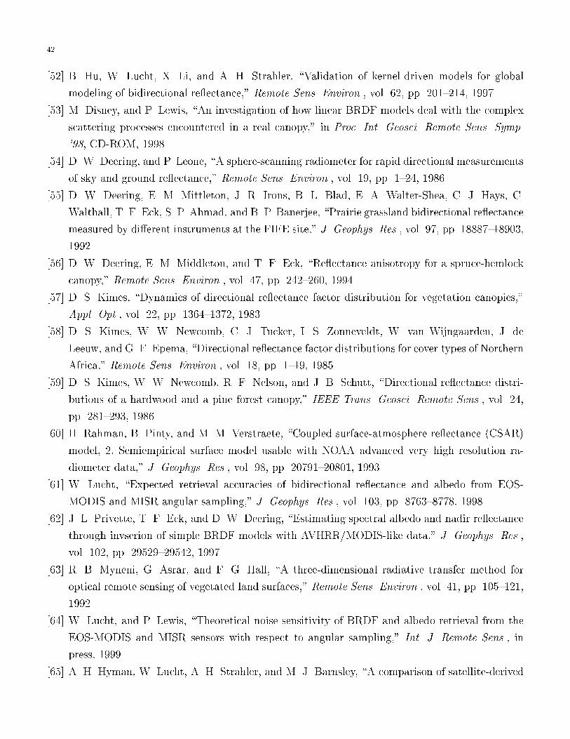
42
[52] B. Hu, W. Lucht, X. Li, and A. H. Strahler, \Validation of kernel-driven models for global
modeling of bidirectional re ectance," Remote Sens. Environ., vol. 62, pp. 201{214, 1997.
[53] M. Disney, and P. Lewis, \An investigation of how linear BRDF models deal with the complex
scattering processes encountered in a real canopy," in Proc. Int. Geosci. Remote Sens. Symp.
'98, CD-ROM, 1998.
[54] D. W. Deering, and P. Leone, \A sphere-scanning radiometer for rapid directional measurements
of sky and ground re ectance," Remote Sens. Environ., vol. 19, pp. 1{24, 1986.
[55] D. W. Deering, E. M. Mittleton, J. R. Irons, B. L. Blad, E. A. Walter-Shea, C. J. Hays, C.
Walthall, T. F. Eck, S. P. Ahmad, and B. P. Banerjee, \Prairie grassland bidirectional re ectance
measured by di�erent instruments at the FIFE site," J. Geophys. Res., vol. 97, pp. 18887{18903,
1992.
[56] D. W. Deering, E. M. Middleton, and T. F. Eck, \Re ectance anisotropy for a spruce-hemlock
canopy," Remote Sens. Environ., vol. 47, pp. 242{260, 1994.
[57] D. S. Kimes, \Dynamics of directional re ectance factor distribution for vegetation canopies,"
Appl. Opt., vol. 22, pp. 1364{1372, 1983.
[58] D. S. Kimes, W. W. Newcomb, C. J. Tucker, I. S. Zonneveldt, W. van Wijngaarden, J. de
Leeuw, and G. F. Epema, \Directional re ectance factor distributions for cover types of Northern
Africa," Remote Sens. Environ., vol. 18, pp. 1{19, 1985.
[59] D. S. Kimes, W. W. Newcomb, R. F. Nelson, and J. B. Schutt, \Directional re ectance distri-
butions of a hardwood and a pine forest canopy," IEEE Trans. Geosci. Remote Sens., vol. 24,
pp. 281{293, 1986.
[60] H. Rahman, B. Pinty, and M. M. Verstraete, \Coupled surface-atmosphere re ectance (CSAR)
model, 2, Semiempirical surface model usable with NOAA advanced very high resolution ra-
diometer data," J. Geophys. Res., vol. 98, pp. 20791{20801, 1993.
[61] W. Lucht, \Expected retrieval accuracies of bidirectional re ectance and albedo from EOS-
MODIS and MISR angular sampling," J. Geophys. Res., vol. 103, pp. 8763{8778, 1998.
[62] J. L. Privette, T. F. Eck, and D. W. Deering, \Estimating spectral albedo and nadir re ectance
through invserion of simple BRDF models with AVHRR/MODIS-like data," J. Geophys. Res.,
vol. 102, pp. 29529{29542, 1997.
[63] R. B. Myneni, G. Asrar, and F. G. Hall, \A three-dimensional radiative transfer method for
optical remote sensing of vegetated land surfaces," Remote Sens. Environ., vol. 41, pp. 105{121,
1992.
[64] W. Lucht, and P. Lewis, \Theoretical noise sensitivity of BRDF and albedo retrieval from the
EOS-MODIS and MISR sensors with respect to angular sampling," Int. J. Remote Sens., in
press, 1999.
[65] A. H. Hyman, W. Lucht, A. H. Strahler, and M. J. Barnsley, \A comparison of satellite-derived

43
spectral albedos to ground-based broadband albedo measurements modelled to satellite spatial
scale for a semi-desert landscape," Remote Sens. Environ., submitted, 1999.
[66] P. Lewis, M. I. Disney, M. J. Barnsley, and J.-P. Muller, \Deriving albedo maps for HAPEX-
Sahel from ASAS data using kernel-driven BRDF models," Hydrol. Earth System Sci., in press,
1999.
[67] A. H. Strahler, W. Wanner, C. B. Schaaf, X. Li, B. Hu, J.-P. Muller, P. Lewis, and M. J. Barnsley,
MODIS BRDF/albedo product: Algorithm theoretical basis document, NASA EOS-MODIS Doc.,
Version 4.0, 252 pp., 1996.
[68] R. E. Wolfe, D. P. Roy, and E. Vermote, \MODIS land data storage, gridding, and compositing
methodology: Level 2 grid," IEEE Trans. Geosci. Remote Sens., vol. 36, pp. 1324-1338, 1998.
[69] D. P. Wylie, and W. P. Menzel, \Two years of cloud cover statistics using VAS," J. Clim., vol.
2, pp. 380{392, 1989.
[70] D. P. Wylie, W. P. Menzel, H. M. Woolf, and K. I. Strabala, \Four years of global cirrus cloud
statistics using HIRS," J. Clim., vol. 7, pp. 1972{1986, 1994.
[71] N. C. Strugnell and W. Lucht, \Continental-scale albedo inferred from AVHRR data, land cover
class and �eld observations of typical BRDFs," J. Clim., submitted, 1999.
[72] I. Guttman, Linear Models: An introduction, John Wylie & Sons, New York, 348 pp., 1982.
[73] R. L. Parker, Geophysical inverse theory, Princeton Univ. Press, Princeton, N.J., 386 pp., 1994.
[74] C. R. Rao, and H. Toutenberg, Linear models: least squares amd alternatives, Springer, New
York, 352 pp., 1995.
[75] J. M. Chen and J. Cihlar, \A hotspot function in a simple bidirectional re ectance model for
satellite applications," J. Geophys. Res., vol. 102, pp. 25907{25913, 1997.
[76] R. E. Dickinson, \Land surface processes and climate { surface albedos and energy balance,"
Advan. Geophys., vol. 25, pp. 305{353, 1983.
[77] B. P. Briegleb, P. Minnis, J. T. Suttles, and R. S. Kandel, \Comparison of regional clear-sky
albedos inferred from satellite observations and model computations," J. Clim. Appl. Meteorol.,
vol. 25, pp. 214{226, 1986.
[78] P. Lewis and E. Vives Ruiz de Lope, \The application of kernel-driven BRDF models and
AVHRR data to monitoring land surface dynamics in the Sahel," J. Remote Sens. (China), vol.
1, Suppl., pp. 155{161, 1997.
[79] B. Hu, W. Lucht, A. Strahler, C. Schaaf, and M. Smith, \Surface albedos and angle-corrected
NDVI from AVHRR observations over South America," Remote Sens. Environ., under revision,
1999b.
[80] R. E. d'Entremont, C. L. Barker Schaaf, W. Lucht, and Alan H. Strahler, \Retrieval of red
spectral albedo and bidirectional re ectance from 1-km**2 satellite observations for the New
England region," J. Geophys. Res., vol. 104, pp. 6229-6239, 1999.

44
[81] P. Minnis, S. Mayor, W. L. Smith, and D. F. Young, \Assymmetry in the diurnal variation of
surface albedo," IEEE Trans. Geosci. Remote Sens., vol. 35, pp. 879{891, 1997.
[82] I. F. Grant, A. J. Prata, and R. P. Cechet, \The impact pf the diurnal variation of albedo on
the remote sensing of the daily mean albedo of grassland," J. Appl. Meteorol., submitted, 1999.
[83] W. Lucht, C. Schaaf, A. H. Strahler, and R. E. d'Entremont, \Remote sensing of albedo using
the BRDF in relation to land surface properties," in Proc. Workshop Opt. Remote Sens. Terrest.
Surf., Tuusula, Finland, in press, 1999.
[84] J. Polcher and K. Laval, \A statistical study of the regional impact of deforestation on climate
in the LMD GCM," Clim. Dyn., vol. 10, pp. 205{219, 1994.
[85] J. Lean, and P. R. Rowntree, \Understanding the sensitivity of a GCM simulation of Amazonian
deforestation to the speci�cation of vegetation and soil characteristics," J. Clim., vol. 10, pp.
1216{1235, 1997.
[86] R. A. Betts, P. M. Cox, S. E. Lee, and F. I. Woodward, \Contrasting physiological and structural
vegetation feedbacks in climate change simulations," Nature, vol. 387, pp. 796{799, 1997.
[87] B. A. Wielicki, B. R. Barkstrom, B. A. Baum, T. P. Charlock, R. N. Green, D. P. Kratz, R.
B. Lee III, P. Minnis, G. L. Smith, T. Wong, D. F. Young, R. D. Cess, J. A. Coakley, Jr., D.
A. H. Crommelynck, L. Donner, R. Kandel, M. D. King, A. J. Miller, V. Ramanathan, D. A.
Randall, L. L. Stowe, and R. M. Welch, \Clouds and the earth's radiant energy system (CERES):
Algorithm overview," IEEE Trans. Geosci. Remote Sens., vol. 36, pp. 1127{1141, 1998.
[88] R. N. Green and G. L. Smith, \Shortwave shape factor inversion of earth radiation budget
observations", J. Atmos. Sci., vol. 48, pp. 390{402, 1991.
XII. FIGURES

45
Mirror BRDF:specular reflectance
Rough water surface BRDF:sunglint reflectance
Gap−driven BRDF (Forest):shadow−driven reflectance
Volume scattering BRDF:leaf/vegetation reflectance
!!!!
!!!!!!!!!!
Fig. 1. Basic reasons for land surface re ectance anisotropy: specular scattering such as sunglint, also observed
where forward-scattering leaves or soil elements are present; radiative transfer-type volumetric scattering by �nite
scatterers (leaves of plant canopies) that are uniformly distributed, potentially nonuniformly inclined and them-
selves have anisotropic re ectance; and geometric-optical surface scattering, which is given by shadow-casting and
mutual obscuration of three-dimensional surface elements, for example of trees in a sparse forest or brushland, or
of clods on a plowed �eld or of rock-strewn deserts. In natural systems, all types of scattering are likely to occur
simultaneously.

46
Fig. 2. Principal plane and cross-principle solar plane plots of the RossThick (upper curves) and LiSparse-R (lower
curves) BRDF model kernel values (arbitrary units; the LiSparse-R kernel values were divided by 2 for better
plotting). The sun is located at positive zenith angles of 0 (dotted lines), 20 (dashed lines), 45 (solid lines), and
70 degrees (dashed-dotted line) solar zenith angle. The parameter h=b of the LiSparse-R kernel was set to 2.0, the
parameter b=r to 1.0.
Fig. 3. The BRDF shapes which the Ross-Li BRDF model acquires under natural conditions on the principal solar
plane for a solar zenith angle of 45 degrees. Left panel: Shape of the BRDF using typical values for the model
parameters. The two solid lines represent the maximal volume scattering and geometric-optical scattering found
for 18 �eld-observed BRDFs representing a wide range of barren and vegetated cover typesin the red and near-
infrared wavebands. The dotted lines are intermediate cases where the parameters take on either their respective
maximal value, half of it, or are zero in all possible combinations. Right panel: Shape of the BRDF using observed
model parameters in the red (solid lines) and near-infrared (dotted lines) wavebands. The datasets used represent
sparse brushlands, dense broadleaf forest, dense barren trees on snow, dense needleleaf forest, sparse grass, dense
grassland, and barren soil (data collected by numerous investigators).
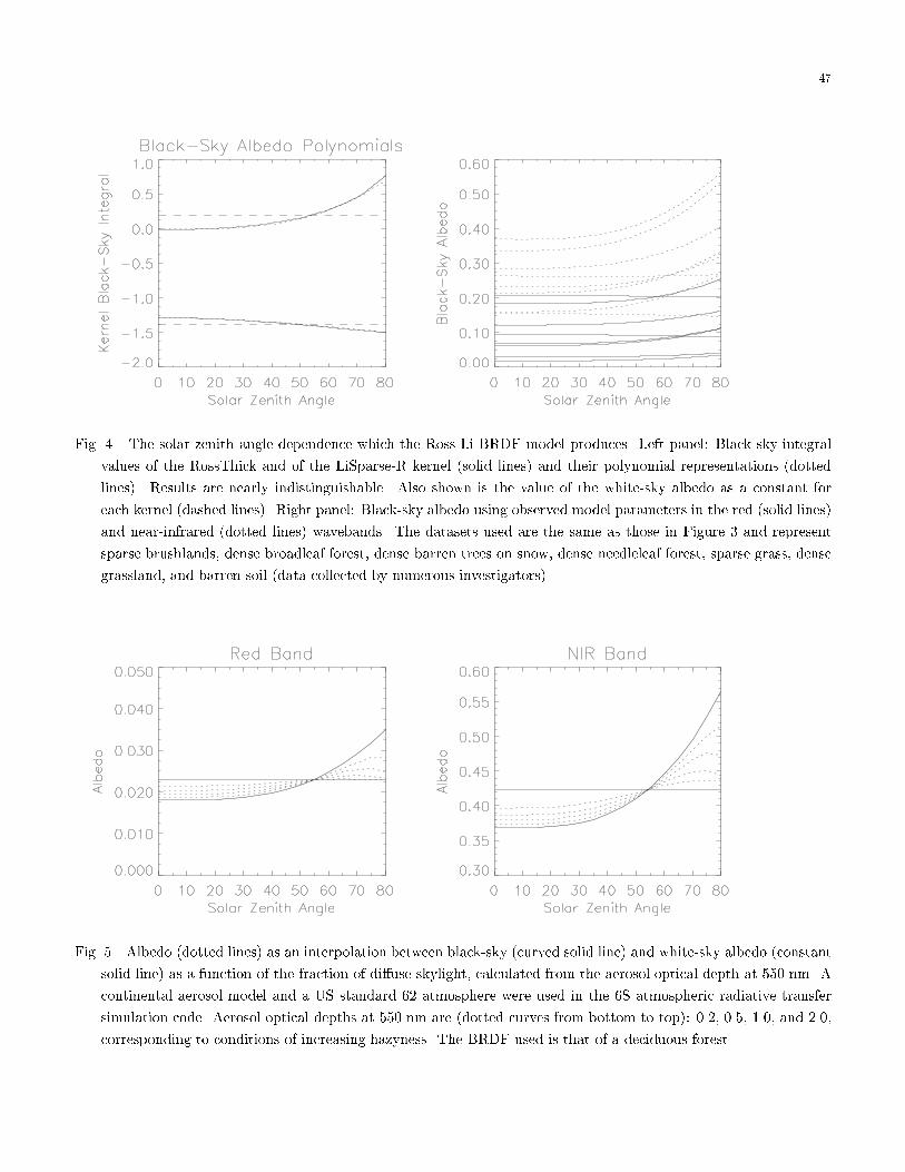
47
Fig. 4. The solar zenith angle dependence which the Ross-Li BRDF model produces. Left panel: Black-sky integral
values of the RossThick and of the LiSparse-R kernel (solid lines) and their polynomial representations (dotted
lines). Results are nearly indistinguishable. Also shown is the value of the white-sky albedo as a constant for
each kernel (dashed lines). Right panel: Black-sky albedo using observed model parameters in the red (solid lines)
and near-infrared (dotted lines) wavebands. The datasets used are the same as those in Figure 3 and represent
sparse brushlands, dense broadleaf forest, dense barren trees on snow, dense needleleaf forest, sparse grass, dense
grassland, and barren soil (data collected by numerous investigators).
Fig. 5. Albedo (dotted lines) as an interpolation between black-sky (curved solid line) and white-sky albedo (constant
solid line) as a function of the fraction of di�use skylight, calculated from the aerosol optical depth at 550 nm. A
continental aerosol model and a US standard 62 atmosphere were used in the 6S atmospheric radiative transfer
simulation code. Aerosol optical depths at 550 nm are (dotted curves from bottom to top): 0.2, 0.5, 1.0, and 2.0,
corresponding to conditions of increasing hazyness. The BRDF used is that of a deciduous forest.
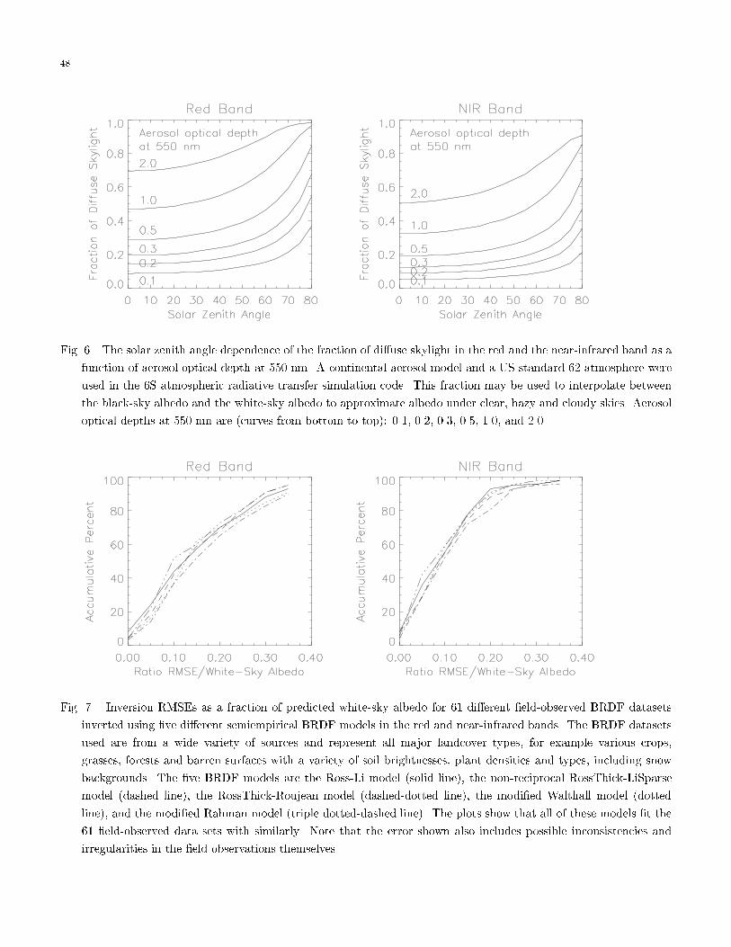
48
Fig. 6. The solar zenith angle dependence of the fraction of di�use skylight in the red and the near-infrared band as a
function of aerosol optical depth at 550 nm. A continental aerosol model and a US standard 62 atmosphere were
used in the 6S atmospheric radiative transfer simulation code. This fraction may be used to interpolate between
the black-sky albedo and the white-sky albedo to approximate albedo under clear, hazy and cloudy skies. Aerosol
optical depths at 550 nm are (curves from bottom to top): 0.1, 0.2, 0.3, 0.5, 1.0, and 2.0.
Fig. 7. Inversion RMSEs as a fraction of predicted white-sky albedo for 61 di�erent �eld-observed BRDF datasets
inverted using �ve di�erent semiempirical BRDF models in the red and near-infrared bands. The BRDF datasets
used are from a wide variety of sources and represent all major landcover types, for example various crops,
grasses, forests and barren surfaces with a variety of soil brightnesses, plant densities and types, including snow
backgrounds. The �ve BRDF models are the Ross-Li model (solid line), the non-reciprocal RossThick-LiSparse
model (dashed line), the RossThick-Roujean model (dashed-dotted line), the modi�ed Walthall model (dotted
line), and the modi�ed Rahman model (triple dotted-dashed line). The plots show that all of these models �t the
61 �eld-observed data sets with similarly. Note that the error shown also includes possible inconsistencies and
irregularities in the �eld observations themselves.

49
Fig. 8. Upper left: Spectra of six di�erent types of landcovers (Source: ASTER spectral library, S.J. Hook). These are
deciduous tree leaves (Dec), conifer needles (Cnf) and grass (Grs) for vegetation (solid lines), a brown silty loam
(BrS) and a dark reddish brown �ne sandy loam (RdS) for soils (dotted lines), and �ne snow (Snw) for snow/ice
(dashed line). Also shown is the solar downwelling spectrum computed with the 6S atmospheric radiative transfer
simulation code using a continental aerosol model and a US standard 62 atmosphere (peaked dashed-dotted line).
Optical depth at 550 nm was 0.2, the sun was at nadir. Symbols mark the location of the MODIS, MISR and
AVHRR spectral bands. Other panels: Comparison of total shortwave, visible and near-infrared broadband albedos
computed exactly (stars) and as derived from values at the location of MODIS (diamonds), MISR (triangles) and
AVHRR (crosses) spectral bands using conversion coe�cients.
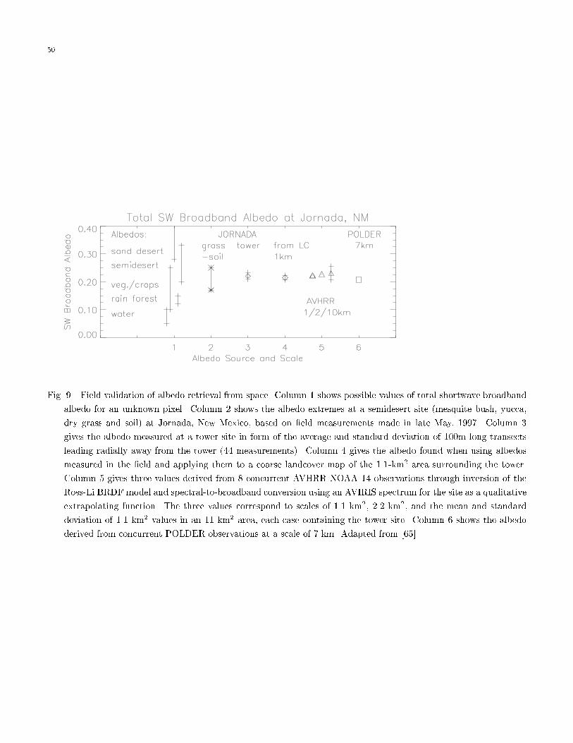
50
Fig. 9. Field validation of albedo retrieval from space. Column 1 shows possible values of total shortwave broadband
albedo for an unknown pixel. Column 2 shows the albedo extremes at a semidesert site (mesquite bush, yucca,
dry grass and soil) at Jornada, New Mexico, based on �eld measurements made in late May, 1997. Column 3
gives the albedo measured at a tower site in form of the average and standard deviation of 100m long transects
leading radially away from the tower (44 measurements). Column 4 gives the albedo found when using albedos
measured in the �eld and applying them to a coarse landcover map of the 1.1-km2 area surrounding the tower.
Column 5 gives three values derived from 8 concurrent AVHRR NOAA 14 observations through inversion of the
Ross-Li BRDF model and spectral-to-broadband conversion using an AVIRIS spectrum for the site as a qualitative
extrapolating function. The three values correspond to scales of 1.1 km2, 2.2 km2, and the mean and standard
deviation of 1.1 km2 values in an 11 km2 area, each case containing the tower site. Column 6 shows the albedo
derived from concurrent POLDER observations at a scale of 7 km. Adapted from [65].
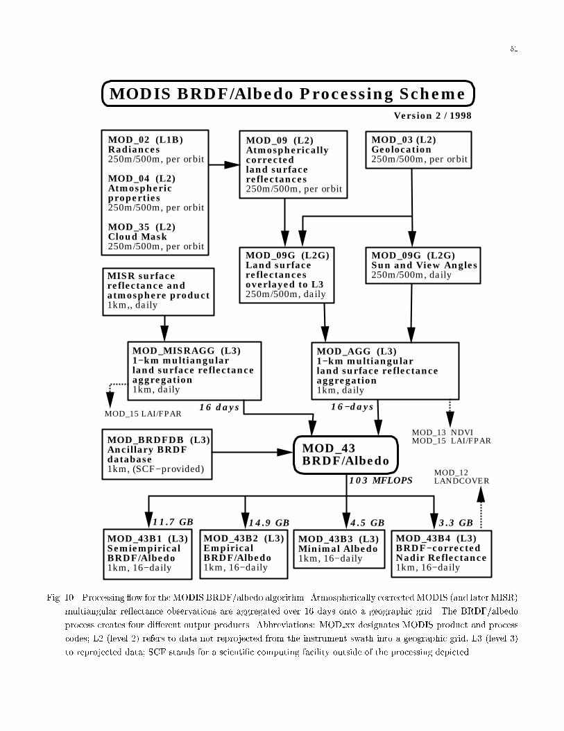
51
Version 2 / 1998
MODIS BRDF/Albedo Processing Scheme
MOD_09G (L2G)Land surface reflectances overlayed to L3250m/500m, daily
MOD_09G (L2G) Sun and View Angles250m/500m, daily
MOD_03 (L2)Geolocation250m/500m, per orbit
MOD_09 (L2)Atmospherically correctedland surfacereflectances250m/500m, per orbit
MISR surface reflectance and atmosphere product1km,, daily
MOD_MISRAGG (L3)1−km multiangular land surface reflectance aggregation1km, daily
MOD_AGG (L3)1−km multiangular land surface reflectance aggregation1km, daily
MOD_BRDFDB (L3)Ancillary BRDFdatabase1km, (SCF−provided)
MOD_43B1 (L3)Semiempirical BRDF/Albedo1km, 16−daily
MOD_43B2 (L3)Empirical BRDF/Albedo1km, 16−daily
MOD_43B3 (L3)Minimal Albedo1km, 16−daily
MOD_43 BRDF/Albedo
MOD_02 (L1B)Radiances250m/500m, per orbit
MOD_04 (L2)Atmosphericproperties250m/500m, per orbit
MOD_35 (L2) Cloud Mask250m/500m, per orbit
MOD_43B4 (L3)BRDF−corrected Nadir Reflectance1km, 16−daily
16−days16 days
103 MFLOPS
11.7 GB 14.9 GB 4.5 GB 3.3 GB
MOD_13 NDVIMOD_15 LAI/FPAR
MOD_12LANDCOVER
MOD_15 LAI/FPAR
Fig. 10. Processing ow for the MODIS BRDF/albedo algorithm. Atmospherically corrected MODIS (and later MISR)
multiangular re ectance observations are aggregated over 16 days onto a geographic grid. The BRDF/albedo
process creates four di�erent output products. Abbreviations: MOD xx designates MODIS product and process
codes; L2 (level 2) refers to data not reprojected from the instrument swath into a geographic grid, L3 (level 3)
to reprojected data; SCF stands for a scienti�c computing facility outside of the processing depicted.

52
(a) Solar Zenith: 0 Degrees (b) Solar Zenith: 45 Degrees
(c) Solar Zenith: 70 Degrees (d) Ratio 45/0 Degrees Solar Zenith
Fig. 11. Black-sky albedo for di�erent solar zenith angles, and the ratio of black-sky albedo at solar zenith angles 45
and 0 degrees. Data derived from co-located NOAA AVHRR-14 and GOES-8 Imager data in the red band with a
nominal spatial resolution of 1 kilometer. Shown is a 400 by 402 km region of New England from September 2 to
18, 1995. Scaling is from 0 to 0.08 (red to yellow) for black-sky albedos at solar zenith angles 0 and 45 degrees,
and from 0 to 0.1 (red to yellow) at solar zenith angle 70 degrees. The ratio image is scaled from 0.8 to 1.8 (blue
to green). Albedos are derived from the multiangular observations using the Ross-Li BRDF model. As the solar
zenith angle of the observations was mostly between 40 and 60 degrees, some of the images are extrapolated in
solar zenith. White-sky albedo is very similar to the black-sky albedo at 45 degrees solar zenith angle. The sun is
never at nadir in September in New England, but this illumination condition is relevant for di�use skylight. The
images clearly show land surface features such as valleys, wooded hills, and large and small cities. The ratio image
shows the spatial variation in the solar zenith angle dependence of albedo with region and land cover. Urban and
disrupted areas show a drop of albedo with solar zenith angle due to shadowing, forested areas an increase.
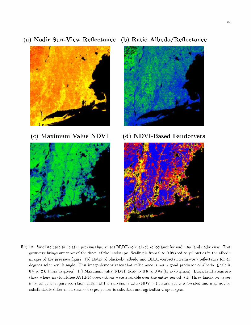
53
(a) Nadir Sun-View Re ectance (b) Ratio Albedo/Re ectance
(c) Maximum Value NDVI (d) NDVI-Based Landcovers
Fig. 12. Satellite data same as in previous �gure. (a) BRDF-normalized re ectance for nadir sun and nadir view. This
geometry brings out most of the detail of the landscape. Scaling is from 0 to 0.08,(red to yellow) as in the albedo
images of the previous �gure. (b) Ratio of black-sky albedo and BRDF-corrected nadir-view re ectance for 45
degrees solar zenith angle. This image demonstrates that re ectance is not a good predictor of albedo. Scale is
0.8 to 2.0 (blue to green). (c) Maximum value NDVI. Scale is 0.8 to 0.95 (blue to green). Black land areas are
those where no cloud-free AVHRR observations were available over the entire period. (d) Three landcover types
inferred by unsupervised classi�cation of the maximum value NDVI. Blue and red are forested and may not be
substantially di�erent in terms of type, yellow is suburban and agricultural open space.