modeling component assembly of a bearing using abaqus

2012 SIMULIA Community Conference 1

Modeling Component Assembly of a Bearing Using Abaqus

Bisen Lin, Ph.D., P.E. and Michael W. Guillot, Ph.D., P.E.

Stress Engineering Services, Inc.

Abstract: Assembly process of a bearing considered in this paper includes: (1) Shrink fit cooling

sleeve into bearing housing with different initial interferences at upper and lower portions of the

interface. (2) Attaching the cooling sleeve to the bearing housing at two ends using welds. (3) Shrink fit bearing sleeve into the assembly of cooling sleeve and bearing housing. Once the bearing is assembled, temperature and pressure loads at desired regions can then be applied.

Simulation techniques used in present work include shrink fits at various analysis steps, model

change (removal and reactivation of parts) at different analysis steps. This will demonstrate the capability of Abaqus in simulating reality of a complex bearing assembly and further stress analysis for different loading conditions.

Moreover, in order to better understand the bearing performance and hence improve the design, a

sensitivity study on the design parameter, different initial interferences at the different interfaces, i.e. cooling sleeve and bearing housing, bearing sleeve and the assembly of cooling sleeve and bearing housing, was conducted.

Keywords: Bearing Assembly, Model Change, Interference Fit, Sensitivity.

1. Introduction

Abaqus has evolved greatly in the past few decades since its first release in 1978. It has a large

variety of modeling techniques, for instance, analysis continuation (restart analysis) technique; sub-modeling technique for a subsequent detailed analysis following a relative coarse-mesh global model analysis; substructure; extended FEM for modeling crack initiation and propagation;

coupled Eulerian-Lagrangian analysis in Abaqus/Explicit, which enables fully coupled multi-physics simulation (e.g. structure-fluid interaction); removal / reactivation of parts of a model

using model change keyword; contact interaction including gradually removing the initial interference; etc.

The capabilities of Abaqus described in this paper were used to help investigate a bearing failure

and to evaluate design changes to minimize future problems. The failure of a seal weld attaching a cooling sleeve in the bearing allowed cooling fluid to leak into the process. This study evaluated the stresses in the seal welds due to the variability in the manufacturing tolerances of the

components in the complex bearing assembly. The results of this sensitivity analysis on the assembly tolerances were used in conjunction with a new weld geometry to reduce the stresses on

the critical seal welds.

u48

Typewritten Text

Visit the Resource Center for more SIMULIA customer papers

http://www.3ds.com/products/simulia/resource-center/

2 2012 SIMULIA Community Conference

Among these advanced modeling techniques, contact interference fit and model change were implemented in a bearing assembly simulation presented in this paper. This simulates the sequential assembly procedures of an actual bearing. In particular, the bearing assembly

considered in this paper includes three layers, i.e. outer layer – bearing housing, intermediate layer – cooling sleeve, and inner layer – bearing sleeve, as well as the top and bottom groove welds

between the outer and middle layers (bearing housing and cooling sleeve). The bearing assembly procedure includes: (1) Assemble bearing housing and cooling sleeve with initial interference at their interfaces on two different diameters. (2) Attach the cooling sleeve and bearing housing

using welds at top and bottom grooves. (3) Shrink fit the inner layer (bearing sleeve) into the assembly of cooling sleeve and bearing housing. Once the three-layer bearing is assembled, temperature boundary conditions and inside bearing pressure can then be applied at the relevant

surfaces. This will demonstrate the capability of Abaqus in simulating reality of a bearing assembly process and subsequent stress analysis.

2. Modeling Techniques

Abaqus modeling techniques used in the bearing assemble study includes removal and reactivation of parts and contact pairs, i.e. model change; and contact interactions with initial interferences.

2.1 Model Change

Special-purpose technique, model change, in Abaqus allows user to remove / reactive elements and/or contact pairs either temporarily or for the remainder of the analysis. Reactivation of

elements can be either strain-free or with strain. The model change technique with strain-free option was used to remove / reactivate the desired bearing parts including welds in the model to simulate the bearing assembly process at different analysis steps.

Following shows examples of Abaqus input usage for removal and reactivation of parts (elements) and contact pair in a model.

Parts (elements) removal:

*MODEL CHANGE, TYPE=ELEMENT, REMOVAL

Element_Set_Name

Parts (elements) strain-free reactivation:

*MODEL CHANGE, TYPE=ELEMENT, ADD

Element_Set_Name

Contact pair removal:

*MODEL CHANGE, TYPE=CONTACT PAIR, REMOVAL

Slave_Surface_Name, Master_Surface_Name

Contact pair reactivation:

*MODEL CHANGE, TYPE= CONTACT PAIR, ADD



2.2 Contact Interference Fit

The automatic shrink fit at the first analysis step and the contact interference fit in the subsequent steps were used to simulate the sequential assemble of the three-layer bearing.

Following shows examples of Abaqus input usage for automatic shrink fit in the first analysis step

and interference fit in other steps for resolving the initial overclosure (interference) between two contact surfaces.

Automatic shrink fit in the first analysis step:

*CONTACT INTERFERENCE, SHRINK


Interference fit in the subsequent steps for resolving initial overclosure:

*CONTACT INTERFERENCE

Slave_Surface_Name, Master_Surface_Name, v

In which, v denotes reference allowable interference. This value is applied instantaneously at the

start of the step and ramped down to zero linearly over the step by default. It is recommended you specify the allowable interference v in a separate step that there are no other loads applied.

Additional loads and/or boundary conditions may adversely affect the resolution of the interference fit and the response to the loading with partially-resolved interferences may be non-physical [1].

3. Abaqus FEA Model

For efficiency and maintaining the model accuracy, an axisymmetric model of the bearing assembly was constructed using Abaqus CAE version 6.10-1. Linear elastic material model was

used. Geometric nonlinearity was incorporated in the model. The four-step assembly process of the bearing is performed followed by the coupled temperature-displacement steady-state analysis.

In this section, details of the FEA model are described. This includes model geometry, finite

element mesh, material properties, tie constraints and contact interaction, as well as boundary conditions and loadings.

3.1 Model Geometry and Mesh

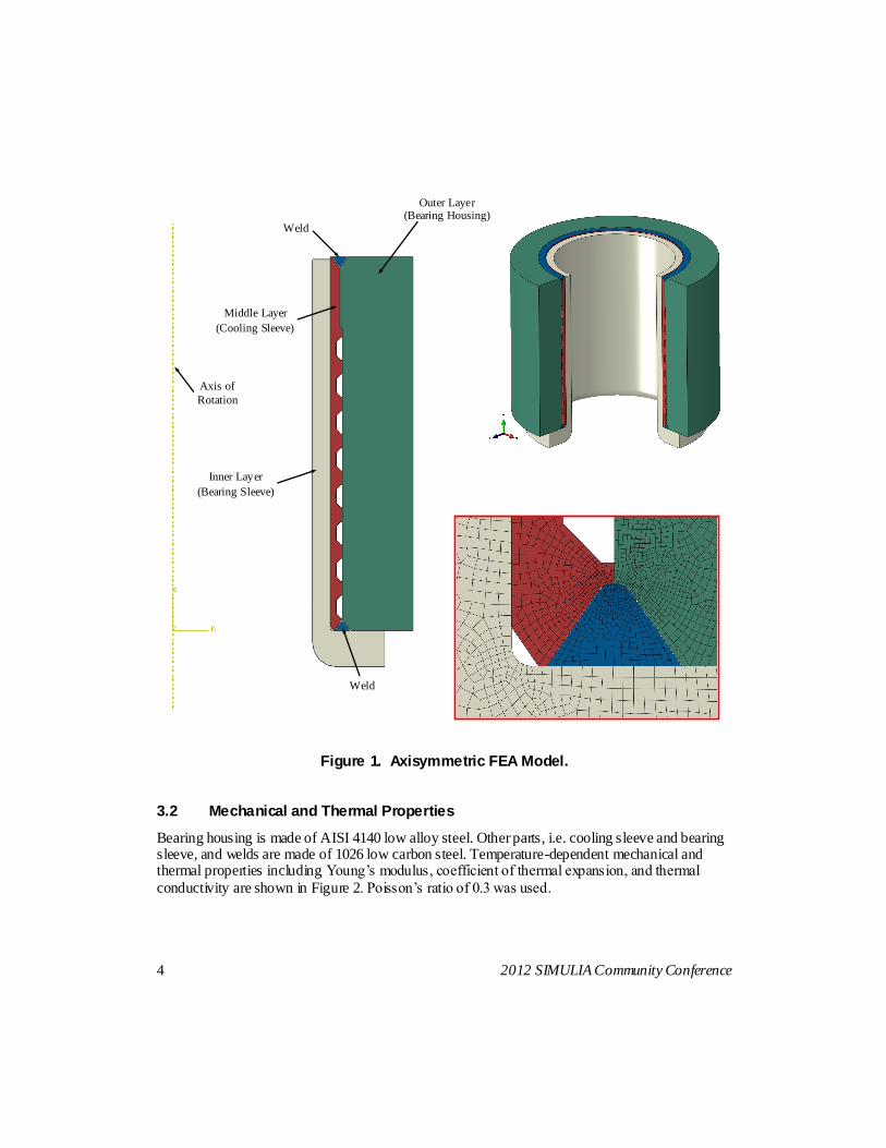
Figure 1 shows the axisymmetric FEA model constructed in Abaqus CAE. Different colors represent different parts. There are four parts in the assembly, i.e. outer layer (bearing housing),

middle layer (cooling sleeve), inner layer (bearing sleeve), and two groove welds between bearing housing and cooling sleeve.

The entire assembly was modeled as CAX4T, a 4-node axisymmetric thermally coupled

quadrilateral element, bilinear in displacement and temperature.


Figure 1. Axisymmetric FEA Model.

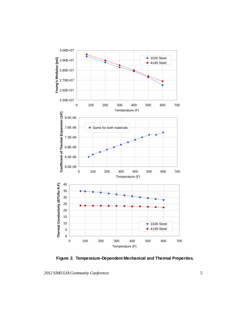
3.2 Mechanical and Thermal Properties

Bearing housing is made of AISI 4140 low alloy steel. Other parts, i.e. cooling sleeve and bearing sleeve, and welds are made of 1026 low carbon steel. Temperature-dependent mechanical and thermal properties including Young’s modulus, coefficient of thermal expansion, and thermal

conductivity are shown in Figure 2. Poisson’s ratio of 0.3 was used.

Axis of

Rotation

Inner Layer

(Bearing Sleeve)

Middle Layer

(Cooling Sleeve)

Weld

Weld

Outer Layer (Bearing Housing)


Figure 2. Temperature-Dependent Mechanical and Thermal Properties.

2.50E+07

2.60E+07

2.70E+07

2.80E+07

2.90E+07

3.00E+07

0 100 200 300 400 500 600 700

Temperature (F)

Yo

un

g's

Mo

du

lus

(p

si) 1026 Steel

4140 Steel

6.0E-06

6.4E-06

6.8E-06

7.2E-06

7.6E-06

8.0E-06

0 100 200 300 400 500 600 700

Temperature (F)

Co

eff

icie

nt

of

Th

erm

al

Ex

pa

ns

ion

(1

/F)

Same for both materials

0

5

10

15

20

25

30

35

40

0 100 200 300 400 500 600 700

Temperature (F)

Th

erm

al

Co

nd

uc

tivit

y (

BT

U/h

r-ft

-F)

1026 Steel

4140 Steel


3.3 Constraints and Interactions

Welds were tied to the bearing housing, and the cooling sleeve using tie constraint in Abaqus. In

addition, interactions at all interfaces were modeled with friction (coefficient of friction = 0.3) and hard contact. A surface-to-surface discretization scheme and finite sliding formulations were used

for all contact pairs. Figure 3 shows locations and identifiers for the three contact interfaces that involve interference fits. In addition, contact interaction was also modeled at the interface where bearing housing and weld sit on the bearing sleeve.

Figure 3. Locations and Identifiers of the Interference Fits.

3.4 Loads and Boundary Conditions

Figure 4 shows the loads and boundary conditions applied in the model. In order to remove the

rigid body motion, lower-outer corner of the bearing housing is restrained in the axial direction (i.e. U2=0 in an Abaqus axisymmetric model). After the model is assembled, combined pressures

and temperature boundary conditions are applied at the relevant regions. Internal bearing pressure and temperature are applied at the inner surface of the bearing sleeve. Upper and lower sections

Int-1

Int-3

Int-1: Upper contact between cooling sleeve

and bearing housing

Int-2: Lower contact between cooling sleeve

and bearing housing

Int-3: Contact between bearing sleeve

and cooling sleeve

Int-2


are insulated. The Dowtherm coolant temperature and pressure are applied in the grooves of the cooling sleeve. Linear-gradient temperature field is applied at the outside surface of the bearing housing. Boundary conditions were obtained from instrumentation on actual bearings in service.

Figure 4. Schematic of Loads and Boundary Conditions.

4. Model Assembly and Analysis Procedure

Figure 5 shows the steps of model assembly procedure and the subsequent stress analysis for a bearing. Specifically, the assembly procedure includes: (1) Assemble bearing housing and cooling sleeve with initial interference at their interfaces. (2) Attach the cooling sleeve and bearing

housing using welds at two end bevels. (3) Shrink fit the inner layer (bearing sleeve) into the assembly of cooling sleeve and bearing housing. Once the three-layer bearing is assembled,

Pressure = 8000 psi

Temperature = 488 F

Insulated

Insulated 380 F

441 F

Pressure = 75 psi

Temperature = 437 F

U2=0


temperature boundary conditions and inside bearing pressure can then be applied at the relevant surfaces.

Figure 5. Assembly and Analysis Flow Chart of a Bearing Model.

5. Sensitivity Study on Initial Interference

Initial interference values at different interfaces are important parameters for optimizing the bearing design, such as reducing stresses in the welds, which enhance the weld fatigue life. Four

different combinations of initial interferences at three interfaces are considered in this paper. These combinations span the manufacturing tolerances for the initial bearing design. Table 1 lists

the initial interference values at three interfaces. As a reference, the length of the bearing housing is 15 inch. Locations and identifiers of the three interference fits are shown in Figure 3.

Step-1. Shrink fit of outer layer (bearing housing) and middle layer

(cooling sleeve)

Step-2. Activations of the welds at two-

end grooves between cooling sleeve

and bearing housing in strain-free state.

Step-3. Activation of the inner layer (bearing sleeve) in strain-free state.

Step-4. Interference fit of bearing

sleeve and the assembly of cooling

sleeve and bearing housing.

Step-5. Applications of loads and thermal boundary conditions for further

stress analysis.


Table 1. Values of Different Initial Interferences.

Case No.

Initial Diametral Interference (inch)

Int-1 (Bearing Housing and

Cooling Sleeve, Upper)

Int-2 (Bearing Housing and

Cooling Sleeve, Lower)

Int-3 (Cooling Sleeve and

Bearing Sleeve)

C-1 0.005 0.005 0.002

C-2 0.005 0 0.002

C-3 0.005 0.005 0.005

C-4 0.005 0 0.005

6. Analysis Results

6.1 Results of Bearing Assembly and C-1

Figure 6 shows the von Mises stress contour plots at four assembly steps for C-1 as listed in Table

1. In particular,

Step-1. Shrink fit cooling sleeve and bearing housing with initial diametral interference equal to 0.005 inch for both Int-1 and Int-2. This induces von Mises stress at a level of

~10ksi in cooling sleeve.

Step-2. Activate groove welds with strain-free condition. Stresses in the welds were verified to be zero.

Step-3. Activate bearing sleeve with strain-free condition. Stresses in the bearing sleeve were verified to be zero.

Step-4. Interference fit bearing sleeve and the assembly of cooling sleeve and bearing housing with initial diametral interference equal to 0.002 inch for Int-3, and 0.002 inch for Int-3. This induces von Mises stress at a level of ~11ksi in bearing sleeve. Meanwhile,

the stress in cooling sleeve is reduced from ~10ksi to ~8ksi and the stress in bearing housing is increased to ~3ksi to ~8ksi.


Figure 6. von Mises Stress Contour at Different Assembly Steps for Case C-1.

Figure 7 shows the contour plots of temperature and von Mises equivalent stress for the loads and

boundary conditions shown in Figure 4 after the 4-step model assembly is completed. Specifically, internal pressure = 8000 psi and internal temperature = 488 F; upper and lower portions of the assembly are insulated; groove pressure = 75 psi and groove temperature = 437 F; linearly

distributed temperature varies from 441 F to 380 F at the outside surface of the bearing housing.

[ psi ]


Figure 7. Temperature and von Mises Stress Contours for Case C-1.

6.2 Results of Sensitivity Study

As described in Section 5, four cases with different combinations of initial interferences were performed. Detailed values of initial interferences are summarized in Table 1. Figure 8 shows the von Mises stress comparison for the four cases. Some observations on looking at the overall

assembly are:

Overall, the assembly in C-2 has the best stress distribution; while the assembly in C-3 has the highest stress regions.

As can be seen in Figure 8 for C-1 and C-2, decreasing the interference at Int-2 (i.e. at lower interface between bearing housing and cooling sleeve) tends to distribute the stress

better and also reduces stresses in bearing housing and sleeve. This is also demonstrated by comparing C-3 to C-1.

As can be seen in Figure 8 for C-1 and C-3, increasing the interference at Int-3 (i.e. at

interface between cooling sleeve and bearing sleeve) tends to increase stresses, especially in bearing housing and cooling sleeve. This can also be observed by comparing C-4 to C-2.

Therefore, reducing the initial interferences at Int-2 and Int-3 will lower the stresses in the assembly including the welds.

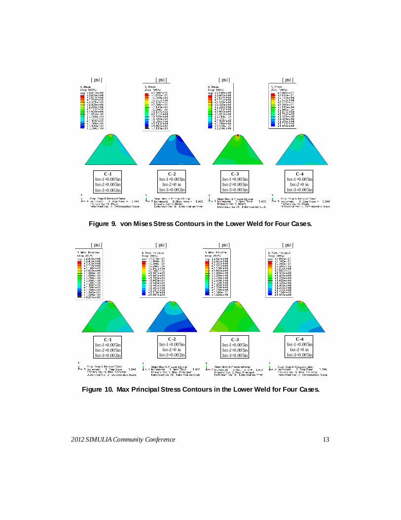
Since the original failure occurred at the lower weld attaching the cooling sleeve to the bearing housing this became the primary area of evaluation. Figure 9 shows the comparison of max

[ psi ] [ ºF ]


principal stress in the lower weld for the four cases. Figure 10 shows the comparison of max principal stress in the lower weld for the four cases. C-2 with zero initial interference at Int-2 and smaller initial interference at Int-3 has the lowest overall stress in the weld although the highly

localized hot-spot stress still exists at the weld tip.

These stress results can then be used in the further structural integrity and component fatigue life

assessments.

Figure 8. von Mises Stress Contours for Four Cases.

[ psi ] [ psi ] [ psi ] [ psi ]

C-1 Int-1=0.005in Int-2=0.005in Int-3=0.002in

C-2 Int-1=0.005in

Int-2=0 in Int-3=0.002in


C-4 Int-1=0.005in



Figure 9. von Mises Stress Contours in the Lower Weld for Four Cases.

Figure 10. Max Principal Stress Contours in the Lower Weld for Four Cases.

[ psi ] [ psi ] [ psi ] [ psi ]

C-1 Int-1=0.005in Int-2=0.005in

Int-3=0.002in

C-2 Int-1=0.005in



C-4 Int-1=0.005in


[ psi ] [ psi ] [ psi ] [ psi ]


C-2 Int-1=0.005in



C-4 Int-1=0.005in



7. Comments and Closures

Modeling of a bearing assembly procedure was considered in this paper using the special techniques in Abaqus, i.e. model change and contact interference fit. The example well

demonstrates the high-quality capability of Abaqus to simulate the reality.

Furthermore, a sensitivity study on the design parameter, i.e. initial overclosure values, was conducted. The results can then be used in the structural integrity and component fatigue life

evaluations of existing equipment or for a new design optimization.

8. References

1. Dassault Systèmes Simulia, “Abaqus Analysis User’s Manual 6.10”, Providence, RI, 2010.

u48

Typewritten Text

Visit the Resource Center for more SIMULIA customer papers

http://www.3ds.com/products/simulia/resource-center/

modeling component assembly of a bearing using abaqus

Documents