Modeling and Control Design for a Magnetic Levitation System

Manfredi Maggiore and Rafael Becerril∗

Department of Electrical and Computer Engineering

University of Toronto, Toronto ON, Canada, M5S 3G4

maggiore@control.utoronto.ca becerril@ece.concordia.ca

Abstract

We study the problem of controlling the position of a platen levitated using linear motors in three-

dimensional space. We develop a nonlinear six-state model of the system and provide two nonlinear

controllers solving the set point stabilization problem. The first controller is derived by decomposing

the model in two subsystems, applying feedback linearization to one of them, and using the invariance

principle to prove attractiveness of the origin of the second subsystem. The second controller is found by

dynamic feedback linearizing the entire system dynamics. In both cases we provide a rigorous procedure

to determine the operating range of the device.

1 Introduction

Recent trends in the semiconductor industry show an increasing need to refine the photo-lithography

process and achieve smaller line-widths (< 0.13µm). Currently in industry the photo-lithography stage is

comprised of a lower-stage that actuates large high-speed movements and a flexure-based upper-stage that

delivers high-precision movements in multiple degrees of freedom (Tsai and Yen 1999). The mechanical

contacts can introduce impurities that may limit the accuracy of the photo-lithography process, thus

decreasing production throughput. Further, the upper-stage flexure mechanism is driven by piezoelectric

actuators that are capable of fine resolution but possess severe hysteresis nonlinearity (Tsai and Yen 1999).

Mechanical contact problems and the inherent nonlinearities of piezoelectric actuators can be avoided by

using planar magnetic levitation technology to move the platen.

Perhaps among the most successful research in this direction is the one reported in (Kim and Trumper

1998), where the authors use a linear controller to actuate a 6 DOF magnetic levitation device that achieves

an x, y, z range of 50mm×50mm×400µm using single sided air cored permanent magnet linear synchronous

∗This work was supported by the Natural Sciences and Engineering Research Council of Canada (NSERC).

Published in International Journal of Control vol.77, 2004, no. 10, pp. 964–977

Platen

y

x

z

Movers

Stators

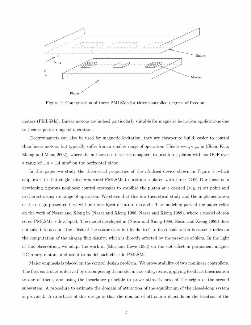
Figure 1: Configuration of three PMLSMs for three controlled degrees of freedom

motors (PMLSMs). Linear motors are indeed particularly suitable for magnetic levitation applications due

to their superior range of operation.

Electromagnets can also be used for magnetic levitation, they are cheaper to build, easier to control

than linear motors, but typically suffer from a smaller range of operation. This is seen, e.g., in (Shan, Kuo,

Zhang and Menq 2002), where the authors use ten electromagnets to position a platen with six DOF over

a range of ±4 ×±4 mm2 on the horizontal plane.

In this paper we study the theoretical properties of the idealized device shown in Figure 1, which

employs three flat single sided iron cored PMLSMs to position a platen with three DOF. Our focus is in

developing rigorous nonlinear control strategies to stabilize the platen at a desired (x, y, z) set point and

in characterizing its range of operation. We stress that this is a theoretical study and the implementation

of the design presented here will be the subject of future research. The modeling part of the paper relies

on the work of Nasar and Xiong in (Nasar and Xiong 1988, Nasar and Xiong 1989), where a model of iron

cored PMLSMs is developed. The model developed in (Nasar and Xiong 1988, Nasar and Xiong 1989) does

not take into account the effect of the stator slots but lends itself to its consideration because it relies on

the computation of the air-gap flux density, which is directly affected by the presence of slots. In the light

of this observation, we adapt the work in (Zhu and Howe 1993) on the slot effect in permanent magnet

DC rotary motors, and use it to model such effect in PMLSMs.

Major emphasis is placed on the control design problem. We prove stability of two nonlinear controllers.

The first controller is derived by decomposing the model in two subsystems, applying feedback linearization

to one of them, and using the invariance principle to prove attractiveness of the origin of the second

subsystem. A procedure to estimate the domain of attraction of the equilibrium of the closed-loop system

is provided. A drawback of this design is that the domain of attraction depends on the location of the

2

permanent magnets

stator

back ironmover

slot

z

x

y

tooth

S

N

LA

Figure 2: Structure of a permanent magnet linear synchronous motor

set point. To overcome this problem, we introduce a dynamic feedback linearizing controller and give

necessary and sufficient conditions for it to make a fixed ellipsoidal set positively invariant for all set points

in an predetermined interval.

2 The model of a PMLSM

In this section we derive a model for a flat single sided iron cored PMLSM made of a short field (or mover)

moving underneath a stationary armature (or stator), as shown in Figure 2. In this device, permanent

magnets occupy the surface of a flat structure of ferromagnetic material –the mover back iron. The stator is

longitudinally laminated and transversally slotted in order to house a three-phase winding. Figure 3 shows

the inertial coordinate frame used in the modeling procedure. As mentioned in the introduction, for this

part we rely on the results of (Nasar and Xiong 1989) and (Zhu and Howe 1993). For the sake of illustration,

we present a brief summary of the derivation of the expressions for the normal and longitudinal forces in a

PMLSM, with emphasis on the differences between our analysis and that in (Nasar and Xiong 1989) and

(Zhu and Howe 1993).

2.1 Magnetic field produced by the permanent magnets

In (Nasar and Xiong 1989), the authors calculate the magnetic potential produced by the permanent

magnets, Ψpm, through the method of images and the concept of magnetic charge. Using the magnetic

charge equivalence, they first describe the magnetic potential around the magnets by means of a system of

partial differential equations. The method of images then solves such system of equations for Ψpm leading

to an expression of the corresponding magnetic field intensity Hpm. Finally, the modeling uses Hpm to

calculate the density of the magnetic flux Bpm around the permanent magnets.

Referring to Figures 2 and 3, let LA be the depth of each permanent magnet along the z axis, hm be

3

x 1i x 2i

t1 b

0

τ τ

g

hmN

S

S

N

N

S

p

y

x

z0

stator

mover

d

Figure 3: Inertial frame used in the analysis of a PMSLM

the height of the magnets, pm the number of permanent magnets, g the air-gap length, t1 the slot pitch,

b0 the slot aperture, τ the permanent magnets pole pitch, τp the permanent magnets pole arc, and σm the

surface magnetic charge. In order to take into account the effect of the slots in the stator, we replace the

air-gap g by the effective air-gap ge, with ge = gKc, where Kc denotes Carter’s coefficient given by

Kc =t1

t1 − gγ1,

γ1 =4

π

b0

2garctan

(

b0

2g

)

− ln

√

1 +

(

b0

2g

)2

.

A simple calculation shows that the position of the kth image of σm is given by

hk =

(k + 1)hm + kge k odd

khm + (k + 1)ge k even

Having found the images’ positions, given an air-gap length g, the method of images yields the y component

of the magnetic field intensity at a point (x0, y0, z0) as follows

Hpmy(x0, y0, z0, g) =σm

4π

pm∑

i=1

∞∑

k=−∞(−1)k+i

[

arctan(x0 − x)(z0 − z)

(y0 − hk)Dk

]

∣

∣

∣

∣

∣

x=x1i

x=x2i

∣

∣

∣

∣

∣

z=LA/2

z=−LA/2

(1)

4

where

Dk =√

(x0 − x)2 + (y0 − hk)2 + (z0 − z)2, x1i =

(

i − 1 + α

2

)

τ, x2i =

(

i − 1 − α

2

)

τ, α =τp

τ.

Since a closed form for (1) cannot be found, we seek a good approximation of it on the surface of the

stator, i.e., when y0 = 0. To this end, we first fix the air-gap length, g = g0, and then average the field

intensity along the z axis. This gives the average field intensity on the stator,

Hg0

pmyav(x0, 0) =2

LA

∫ LA/2

0Hpmy(x0, y0 = 0, z0, g = g0)dz0.

When numerically evaluating this expression for different values of x0, it is found that Hg0pmyav closely resem-

bles a sinusoid. Hence, a first order Fourier series approximation can replace Hg0pmyav without considerable

loss of accuracy. The first Fourier coefficient is given by

Hg0

pmy1 =4

τ

∫ nτ+τ/2

nτHg0

pmyav(x0, 0) sin(π

τx0

)

dx0,

where n = pm

2 with pm the number of poles in the mover. Next, let µ0 be the permeability of free space.

Since in the air-gap Bpm = µ0Hpm, the approximation of the y component of the flux density due to the

permanent magnets is

Bg0

pmy(x0) ' Bg0

pmy1 sin(π

τx0

)

:= µ0Hg0

pmy1 sin(π

τx0

)

.

Recall that this expression holds for a fixed air-gap length g0. Since levitation involves a variable air-gap

length, Bpmy becomes a function of (x0, g0). We incorporate a variable air-gap by calculating the coefficient

µ0Hg0

pmy1 for different values of g0 over the range of interest, and performing a polynomial interpolation to

obtain a function µ0Hpmy1(g0). This gives

Bpmy(x0, g0) ' C1(g0) sin(π

τx0

)

:= µ0Hpmy1(g0) sin(π

τx0

)

.

2.2 Magnetic field produced by the stator

The stator of a PMLSM hosts three phase single layer winding producing a traveling magnetic field. Let

Ia, Ib, and Ic be the phasors of the phase currents and Ia, Ib, and Ic be their magnitudes. Denote the

corresponding instantaneous currents by ia, ib, and ic, such that ia(t) ≤ Ia, ib(t) ≤ Ib, and ic(t) ≤ Ic. Let

d denote relative displacement of the mover with respect to the stator, as illustrated in Figure 3. Let id and

iq denote the direct and quadrature currents associated with the three phase currents ia, ib, and ic. Then,

5

we have

id

iq

=2

3

cos(πτ d) cos

(

πτ d − 2π

3

)

cos(

πτ d + 2π

3

)

− sin(πτ d) − sin

(

πτ d − 2π

3

)

− sin(

πτ d + 2π

3

)

ia

ib

ic

ia + ib + ic = 0.

Further,

id = Ia cos(π

τd)

, iq = −Ia sin(π

τd)

.

Let W be the number of turns of wire on each phase, p the number of pairs of poles in the stator, wc the

coil pitch, and kw1 the first component of the winding factor, given by

kw1 =sin

(

π6

)

wc

3t1sin

(

πt12τ

) sin(πwc

2τ

)

.

Following (Nasar and Xiong 1989) or (Gieras and Piech 2000), the fundamental component of the magneto-

motive force is given by

Fs1(x) = Fs1 sin(π

τx)

=6√

2Wkw1

πKcpIa sin

(π

τx)

.

Fs1 serves as boundary condition for the PDE associated with the first harmonic of the magnetic potential.

The solution to such PDE yields the x and y components of the first harmonic of the magnetic flux density

in the stator

Bs1x(x, y, g) = −C2(y, g) cos(π

τx)

:= −µ0π

τFs1

sinh[

πτ (hm + g − y)

]

sinh[

πτ (hm + g)

] cos(π

τx)

(2)

Bs1y(x, y, g) = −C3(y, g) sin(π

τx)

:= −µ0π

τFs1

cosh[

πτ (hm + g − y)

]

sinh[

πτ (hm + g)

] sin(π

τx)

.

2.3 Slots effect

The difference in reluctance between the slots and the teeth of the stator (see Figure 4) affects the perfor-

mance of the system in two different ways (Zhu and Howe 1993). First, it attenuates the magnetic field in

the air-gap, reducing the magnitude of the forces. This phenomenon is equivalent to having an effective

air-gap length larger than the actual one. Second, the slots spatially modulate the field because the flux

lines travel through low reluctance regions (the teeth). A magnetic model accounts for the first effect

by introducing Carter’s coefficient and the effective air-gap (as seen in Section 2.1) and for the second

effect by calculating the relative permeance of the stator, derived next by adapting the results in (Zhu and

Howe 1993) to PMLSMs. According to (Zhu and Howe 1993), to take into account the presence of slots,

6

b0

2

b0

2

b0

2

b0

2t 1

g

b0t1

x

g(x)

0

g

N

S

-

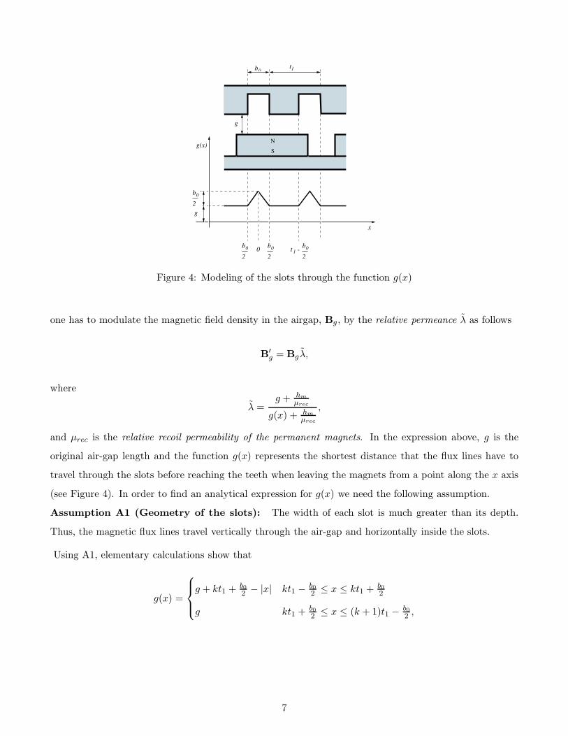
Figure 4: Modeling of the slots through the function g(x)

one has to modulate the magnetic field density in the airgap, Bg, by the relative permeance λ as follows

B′g = Bgλ,

where

λ =g + hm

µrec

g(x) + hm

µrec

,

and µrec is the relative recoil permeability of the permanent magnets. In the expression above, g is the

original air-gap length and the function g(x) represents the shortest distance that the flux lines have to

travel through the slots before reaching the teeth when leaving the magnets from a point along the x axis

(see Figure 4). In order to find an analytical expression for g(x) we need the following assumption.

Assumption A1 (Geometry of the slots): The width of each slot is much greater than its depth.

Thus, the magnetic flux lines travel vertically through the air-gap and horizontally inside the slots.

Using A1, elementary calculations show that

g(x) =

g + kt1 + b02 − |x| kt1 − b0

2 ≤ x ≤ kt1 + b02

g kt1 + b02 ≤ x ≤ (k + 1)t1 − b0

2 ,

7

where k is the index of each slot, b0 its width and t1 its pitch. Since g(x) is a periodic and piecewise

continuous function, in what follows we use the fundamental component of its Fourier expansion

λ ' 1 − b20

4t1(g + b02 + hm

µrec). (3)

2.4 Forces calculation

The superposition of the permanent magnets and the winding field densities yields the resultant field density

in the air-gap. After incorporating the relative permeance, the resultant field density leads to expressions

for the forces in the machine. Our development follows (Nasar and Xiong 1989) but it incorporates a

variable air-gap length.

2.4.1 Longitudinal Force

The longitudinal force depends on the magnetic charge and also on the x component of the traveling

magnetic field in (2), which in turn is affected by the relative permeance given in (3). Given a magnetic

charge σm distributed over a surface S, its interaction with the stator magnetic flux density produces a

longitudinal force

Fx = σm

∫

S

λBsxdS,

where Bsx is the x component of Bs. Letting S be the surface of the top faces of the permanent magnets

and approximating Bsx by its first harmonic in (2) we obtain (refer to Figure 3)

Fx ' pmLAσm

∫ d+τ/2+τp

2

d+τ/2− τp

2

λBs1x(x, y = g, g)dx

= −pmLAσmµ0πτ Fs1λ sinh

(

πτ hm

)

sinh(

πτ (hm + g)

)

∫ d+τ/2+τp

2

d+τ/2− τp

2

cos(π

τx)

dx

= K1(g)Ia sin(π

τd)

= −K1(g)iq,

(4)

where

K1(g) = 12√

2Wkw1pmLAσmµ0λ sinh

(

πτ hm

)

πKcp sinh(

πτ (hm + g)

) sin(πτp

2τ

)

,

and λ is given by (3).

8

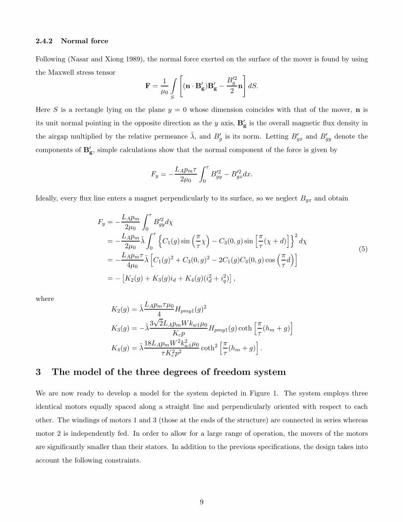
2.4.2 Normal force

Following (Nasar and Xiong 1989), the normal force exerted on the surface of the mover is found by using

the Maxwell stress tensor

F =1

µ0

∫

S

[

(n ·B′g)B′

g−

B′2g

2n

]

dS.

Here S is a rectangle lying on the plane y = 0 whose dimension coincides with that of the mover, n is

its unit normal pointing in the opposite direction as the y axis, B′g

is the overall magnetic flux density in

the airgap multiplied by the relative permeance λ, and B′g is its norm. Letting B′

gx and B′gy denote the

components of B′g, simple calculations show that the normal component of the force is given by

Fy = −LApmτ

2µ0

∫ τ

0B′2

gy − B′2gxdx.

Ideally, every flux line enters a magnet perpendicularly to its surface, so we neglect Bgx and obtain

Fy = −LApm

2µ0

∫ τ

0B′2

gydχ

= −LApm

2µ0λ

∫ τ

0

C1(g) sin(π

τχ)

− C3(0, g) sin[π

τ(χ + d)

]2dχ

= −LApmτ

4µ0λ

[

C1(g)2 + C3(0, g)2 − 2C1(g)C3(0, g) cos(π

τd)]

= −[

K2(g) + K3(g)id + K4(g)(i2d + i2q)]

,

(5)

where

K2(g) = λLApmτµ0

4Hpmy1(g)2

K3(g) = −λ3√

2LApmWkw1µ0

KcpHpmy1(g) coth

[π

τ(hm + g)

]

K4(g) = λ18LApmW 2k2

w1µ0

τK2c p2

coth2[π

τ(hm + g)

]

.

3 The model of the three degrees of freedom system

We are now ready to develop a model for the system depicted in Figure 1. The system employs three

identical motors equally spaced along a straight line and perpendicularly oriented with respect to each

other. The windings of motors 1 and 3 (those at the ends of the structure) are connected in series whereas

motor 2 is independently fed. In order to allow for a large range of operation, the movers of the motors

are significantly smaller than their stators. In addition to the previous specifications, the design takes into

account the following constraints.

9

Fy1 Fy1Fy2

Fz Fz

Motor 1 Motor 2 Motor 3

Fx

stators

movers

xz

y

δx

g

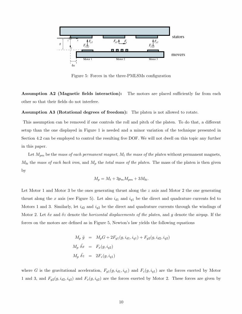
Figure 5: Forces in the three-PMLSMs configuration

Assumption A2 (Magnetic fields interaction): The motors are placed sufficiently far from each

other so that their fields do not interfere.

Assumption A3 (Rotational degrees of freedom): The platen is not allowed to rotate.

This assumption can be removed if one controls the roll and pitch of the platen. To do that, a different

setup than the one displayed in Figure 1 is needed and a minor variation of the technique presented in

Section 4.2 can be employed to control the resulting five DOF. We will not dwell on this topic any further

in this paper.

Let Mpm be the mass of each permanent magnet, Mt the mass of the platen without permanent magnets,

Mbi the mass of each back iron, and Mp the total mass of the platen. The mass of the platen is then given

by

Mp = Mt + 3pmMpm + 3Mbi.

Let Motor 1 and Motor 3 be the ones generating thrust along the z axis and Motor 2 the one generating

thrust along the x axis (see Figure 5). Let also id1 and iq1 be the direct and quadrature currents fed to

Motors 1 and 3. Similarly, let id2 and iq2 be the direct and quadrature currents through the windings of

Motor 2. Let δx and δz denote the horizontal displacements of the platen, and g denote the airgap. If the

forces on the motors are defined as in Figure 5, Newton’s law yields the following equations

Mp g = MpG + 2Fy1(g, id1, iq1) + Fy2(g, id2, iq2)

Mp δx = Fx(g, iq2)

Mp δz = 2Fz(g, iq1)

where G is the gravitational acceleration, Fy1(g, id1, iq1) and Fz(g, iq1) are the forces exerted by Motor

1 and 3, and Fy2(g, id2, iq2) and Fx(g, iq2) are the forces exerted by Motor 2. These forces are given by

10

expressions (4) and (5). Letting

x = [g, g, δx, ˙δx, δz, δz]>, u = [iq1, iq2, id1, id2]>

we get the state space model

x1 = x2

x2 = G − L4(x1)[2u21 + u2

2 + 2u23 + u2

4] − L3(x1)[2u3 + u4] − 3L2(x1)

x3 = x4

x4 = −L1(x1)u2

x5 = x6

x6 = −2L1(x1)u1.

(6)

where Li(x1) :=Ki(x1)

Mp, i = 1, . . . , 4.

4 Nonlinear Control Design

In this section we investigate the set-point stabilization problem for system (6) through two nonlinear

approaches.

4.1 Lyapunov-Based Design

Let xd = [xd1, 0, x

d2, 0, x

d3, 0]

> be the desired set-point and define

x = x− xd, x1 = [x1, x2]>, x2 = [x3, . . . , x6]

>.

Next, consider the controller

u1

u2

=

0 − 12L1(x1)

− 1L1(x1)

0

v1(x2)

v2(x2)

u3 = 0

u4 = −L3(x1) +√

R(x)

2L4(x1)

(7)

where

R(x) = [L3(x1)]2 + 4L4(x1)

[

ε (x1 + x2) (x21 + x2

2) + x2 − L4(x1)U(x) + G − 3L2(x1)]

v1(x2)

v2(x2)

= −Kx2, U(x) = 2

(

v2(x2)

2L1(x1)

)2

+

(

v1(x2)

L1(x1)

)2

,(8)

11

K is a 2 × 4 matrix and ε > 0. The controller above is well-defined on the set

D = (x1, x2) ∈ R2 × R

4 : R(x) ≥ 0, L4(x1) 6= 0, L1(x1) 6= 0,

and the closed-loop system reads as

x1 :

˙x1 = x2

˙x2 = −ε (x1 + x2) [x21 + x2

2] − x2

(9)

˙x2 = (Ac − BcK)x2. (10)

where the pair (Ac, Bc) is in Brunovsky normal form. Choose K so that Ac − BcK is Hurwitz. Clearly, if

L1(x1) 6= 0, u1 and u2 are well-defined and the x2 subsystem is exponentially stable. Let P be the positive

definite matrix satisfying

(Ac − BcK)>P + P (Ac − BcK) = −I,

so that, letting V 2 = x2>P x2, the set Ω2d = x2 : V 2(x2) ≤ d is positively invariant for any d ≥ 0. Next,

consider the Lyapunov function candidate V 1(x1) = 12 x2

1 + 12 (x1 + x2)

2 whose derivative is given by

V 1(x1) = −x21 + x1(x1 + x2) − ε(x1 + x2)

2[x21 + x2

2]

≤ − x21

2−

ε[

x21 + x2

2

]

− 1

2

(x1 + x2)2.

V 1(x1) is negative outside the ball D =

x1 ∈ R2 : x2

1 + x22 ≤ 1

2ε

. Let

Ω1d = x1 ∈ R

2 : V 1(x1) ≤ d

and notice that d∗ = 3+√

58ε is the smallest real number guaranteeing that D ⊂ Ω1

d. In other words,

V 1 ≥ d∗ ⇒ V 1 ≤ 0,

and thus Ω1d is positively invariant for all d ≥ d∗.

Consider now the function W (x1) = (x1+x2)2

2 , then

W (x1) = −ε(x1 + x2)2(x2

1 + x22) ≤ 0,∀x1 ∈ R

2.

Let E = x1 ∈ Ω1d : W (x1) = 0 = x1 ∈ Ω1

d : (x1 + x2) = 0. For any trajectory in E, the dynamics of

12

(9) are given by

˙x1 = −x1

˙x2 = −x2.(11)

Hence, on E, ˙x1 + ˙x2 = 0, showing that E is invariant. Applying LaSalle’s theorem, we conclude that,

for all d ≥ d∗, every integral curve of (9) leaving from Ω1d approaches E as t → ∞. Moreover, from (11),

x1 → 0 on E. Since Ω1d is compact, all trajectories are bounded and it follows that, for all x1(0) ∈ Ω1

d,

x1(t) → 0. Again, this holds for all d such that d > d∗.

We now seek to find an estimate of the domain of attraction of the origin x = 0. This can be

accomplished, in principle, by numerically finding the largest real numbers d1 and d2 such that

Ω1d1

× Ω2d2

⊂ D = (x1, x2) ∈ R2 × R

4 : R(x) ≥ 0, L4(x1) 6= 0, L1(x1) 6= 0,

but this is computationally too hard. The problem can be significantly simplified by finding an upper

bound to R(x) in (8) which depends only on x1. If that can be done, the estimation of the domain of

attraction can be easily carried out numerically on the (x1, x2) plane. From (8), it is clear that finding an

upper bound to

`(x2) = v1(x2)2 +

v2(x2)2

2

gives a lower bound on R(x) which depends only on x1. Assume that x2(0) ∈ Ω2d2

, for some d2 > 0,

so that x2(t) ∈ Ω2d2

for all t ≥ 0. Recall that [v1, v2]> = −Kx2, where K is a 2 × 4 matrix, and let

K ′ = diag[1, 1/√

2]K. Then, `(x2) = x2>K ′>K ′x2 and its upper bound is given by

maxΩ2

d2

x2>K ′>K ′x2

= maxx2>P x2≤d2

x2>K ′>K ′x2

.

This constrained optimization problem can be solved analytically. From the Khun-Tucker necessary con-

ditions we have that extrema are either points in the interior of Ω2d2

such that ∇` = 0, i.e.,

K ′>K ′x2 = 0 ⇐⇒ x2 ∈ ker(K ′>K ′),

for which `(x2) = 0, or points on the boundary of Ω2d2

such that ∇` is parallel to the gradient of the

constraint, i.e.,

(i) K ′>K ′x2 = λP x2 ⇐⇒ (K ′>K ′ − λP )x2 = 0

(ii) x2>P x2 = d2,

for some real number λ. Using the Cholesky decomposition of P , P = LL>, with L invertible, condition

13

(i) can be rewritten as

(K ′>K ′ − λP )x2 = 0 ⇐⇒ (K ′>K − λLL>)x2 = 0

⇐⇒ (L−1K ′>K ′L−> − λI)L>x2 = 0.

Hence, for condition (i) to be satisfied, λ must be an eigenvalue of L−1K ′>K ′L−> (or, equivalently, an

eigenvalue of P−1K ′>K ′) and, letting v be the eigenvector associated to λ with ‖v‖ = 1, x2 must solve

L>x2 = µv, for some real number µ. So one must have x2 = µL−>v. Notice that all eigenvalues of

L−1K ′>K ′L−> are real and nonnegative.

Next, for condition (ii) to be satisfied, one must have

µ2v>L−1PL−>v = d2 ⇐⇒ µ2v>L−1(LL>)L−>v = d2

⇐⇒ µ2 = d2.

Then, the corresponding value of ` is

`(x2) = `(µL−>v) = d2v>(L−1K ′>K ′L−>v)

= d2v>(λv)

= d2λ.

In conclusion, the maximum value of ` is given by

maxΩ2

d2

`(x2) = max

0, d2 λmax(L−1K ′>K ′L−>)

= d2 λmax(P−1K ′>K ′). (12)

This result is used in the following procedure to determine an estimate of the domain of attraction of

x = 0.

14

Procedure 1: Estimation of the domain of attraction of x = 0

1. Numerically find the set X1 = x1 : L3(x1)2 + 4L4(x1)(G − 3L2(x1)) > 0, L4(x1) 6= 0, L1(x1) 6= 0

2. Choose the set point for the air-gap in this set, i.e., choose xd1 ∈ X1

3. Choose K ∈ R2×4 such that the pair Ac − BcK is Hurwitz

4. Set U∗ =(

L1(xd

1)

2L4(xd

1)

)2(

L3(xd1)

2 + 4L4(xd1)G − 12L4(x

d1)L2(x

d1)

)

, and choose U ∈ (0, U∗). Find the feasible

horizontal operating range for the platen:

(a) Let K ′ = diag[1, 1/√

2]K

(b) Set d2 = U/λmax(P−1K ′>K ′). The horizontal operating range is x2 ∈ Ω2d2

5. Choose ε > 0 in (8) and find (possibly the largest) d1 > 0 such that

Ωd1⊂ D = x1 ∈ R

2 : R(x1) ≥ 0, L4(x1) 6= 0, L1(x1) 6= 0

R(x1) = L3(x1)2 + 4L4(x1)

(

ε (x1 + x2) (x21 + x2

2) + x2 −L4(x1)

[L1(x1)]2U + G − 3L2(x1)

)

6. Check whether ε ≥ 2+√

58d1

. If not, repeat item 5 with some other choice of ε. If yes, the feasible vertical

operating range for the platen is x1 ∈ Ω1d1

Lemma 1 Let xd1 be any point in the set X1 defined in item 1 of the procedure. If there exists ε satisfying

the requirement in item 6, then any integral curve of the closed-loop system (6), (7) leaving from a point

in the set Ω1d1

× Ω2d2

is bounded and asymptotically approaches the equilibrium x = xd.

Remark 1: Note that the result in Lemma 1 guarantees boundedness of x and attractiveness of the

equilibrium xd, but not Lyapunov stability.

Proof of Lemma 1: We primarily need to show that every integral curve of (9), (10) leaving from

Ω1d1×Ω2

d2, with d1 and d2 defined in the procedure above, is entirely contained in the set D. By the choice

of xd1, U∗ defined in item 4 of the procedure is such that

Ψ(U∗)4= L3(x1)

2 + 4L4(x1)

(

− L4(xd1)

[L1(xd1)]

2U∗ + G − 3L2(x1)

)

= 0.

Since L4(xd1) 6= 0 and L1(x

d1) 6= 0, for any U ∈ (0, U∗) we have Ψ(U) > 0. Thus, for all xd

1 ∈ X1 and all

U ∈ (0, U∗), R([0 0]>) > 0, implying that Ω10 ⊂ int D. By the continuity of R(·), L4(·), and L1(·), there

exists a positive real number d1 satisfying the requirement in item 5 of the procedure. By the definition of

15

d2 in item 4, the set Ω2d2

is positively invariant and

maxΩ2

d2

(

v21 +

v22

2

)

= U .

Thus, for any x2(0) ∈ Ω2d2

, R(x(t)) ≥ R(x1(t)). If ε satisfies item 6 of the procedure, then d1 ≥ 3+√

58ε ,

implying that Ω1d1

is positively invariant. Thus we obtain

x1(0) ∈ Ω1d1

and x2(0) ∈ Ω2d2

⇒ x1(t) ∈ D ∀t ≥ 0

⇒ x(t) ∈ D ∀t ≥ 0.

In conclusion, if x(0) ∈ Ω1d1

× Ω2d2

, the controller (7) is well-defined for all t ≥ 0 and the solution x(t)

approaches the origin.

Remark 2: The procedure outlined above can easily be implemented numerically, as it requires studying

the sign of a function over the real line (item 1) and one function over the plane (item 5). Note, however,

that we do not provide an algorithm to choose ε. The simulations in Section 5.1 indicate that there is a

wide range of values of ε satisfying the requirement in item 6.

4.2 Dynamic Feedback Linearization

The main drawback of the control design presented in the previous section is that the size of the domain

of attraction of the equilibrium xd depends on the choice of xd1 (but it does not depend on the choice of

xd3 and xd

5). In practice it is desirable to have a guaranteed range of operation which is independent of the

set point. To address this problem, we replace the function R(x) in (7) by the following dynamic feedback

linearizing controller

R(x, z) = L3(x1)2 + 4L4(x1) (−z − L4(x1)U(x) + G − 3L2(x1))

z = −k1x1 − k2x2 − k3z,(13)

with U(·) defined as in (8). With this choice, the closed-loop dynamics read as

x1 :

˙x1 = x2

˙x2 = z

z = −k1x1 − k2x2 − k3z

(14)

x2 : x2 = (Ac − BcK)x2, (15)

16

where k1, k2, k3 are chosen so that the matrix

A =

0 1 0

0 0 1

−k1 −k2 −k3

is Hurwitz. As before, the vector field (14), (15) is well-defined as long as

(x(t), z) ∈ D = (x, z) ∈ R6 × R : R(x, z) ≥ 0, L4(x1) 6= 0, L1(x1) 6= 0.

By using a dynamic feedback we ensure that R(x, z) does not directly depend on u, which makes it possible

to find an estimate of the domain of attraction of the closed-loop system independently of xd1. To this end,

we adapt the idea developed in the previous section and define the inner approximation to the projection

of D onto the (x1, x2, z) coordinates

D =

(x1, x2, z) ∈ R3 : R(x1, x2, z) ≥ 0, L4(x1) 6= 0, L1(x1) 6= 0

R(x1, x2, z) = L3(x1)2 + 4L4(x1)

(

−z − L4(x1)

[L1(x1)]2U + G − 3L2(x1)

)

.

Similarly to what we had earlier, letting d2 = U/λmax(P−1K ′>K ′), the following holds

(x1, x2, z) ∈ D and x2 ∈ Ω2d2

⇒ x ∈ D,

hence, to guarantee that (14), (15) are well-defined, we need to design a controller for (14) guaranteeing

that (x1(t), x2(t), z(t)) ∈ D for all t ≥ 0 and (x1(t), x2(t)) → 0.

Let H be a 3× 3 positive definite matrix, C be a 3× 1 vector, and R a positive real number such that

the ellipsoid centered at C

N =

(x1, x2, z) ∈ R3 : [x1 − C1 x2 − C2 z − C3]H[x1 − C1 x2 − C2 z − C3]

> ≤ R

(16)

is contained in D. Letting ξ = (x1 + xd1 − C1, x2 −C2, z − C3), N is expressed in (x1, x2, z) coordinates as

N =

(x1, x2, z) ∈ R3 : ξ>Hξ ≤ R

.

For a choice of xd1, k1, k2, and k3, the next lemma gives necessary and sufficient conditions for N to be

positively invariant.

17

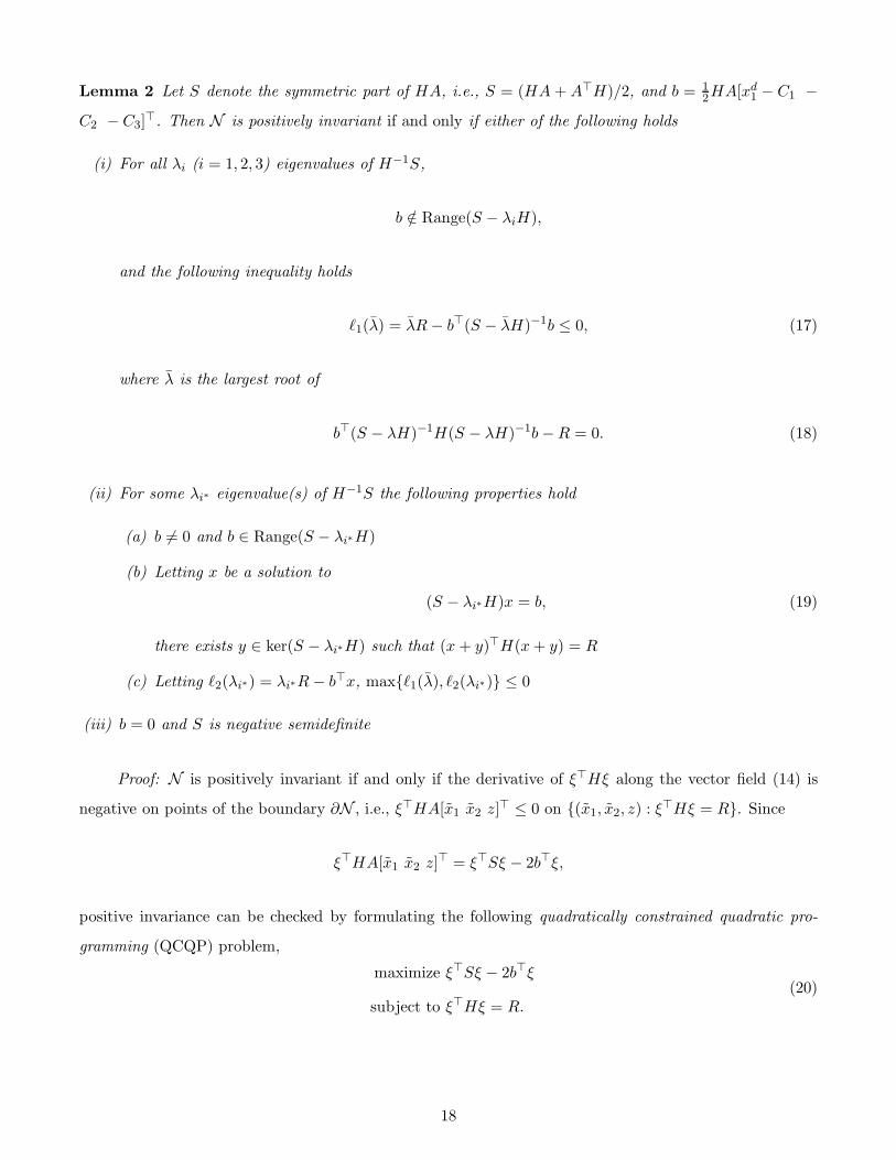
Lemma 2 Let S denote the symmetric part of HA, i.e., S = (HA + A>H)/2, and b = 12HA[xd

1 − C1 −C2 − C3]

>. Then N is positively invariant if and only if either of the following holds

(i) For all λi (i = 1, 2, 3) eigenvalues of H−1S,

b /∈ Range(S − λiH),

and the following inequality holds

`1(λ) = λR − b>(S − λH)−1b ≤ 0, (17)

where λ is the largest root of

b>(S − λH)−1H(S − λH)−1b − R = 0. (18)

(ii) For some λi∗ eigenvalue(s) of H−1S the following properties hold

(a) b 6= 0 and b ∈ Range(S − λi∗H)

(b) Letting x be a solution to

(S − λi∗H)x = b, (19)

there exists y ∈ ker(S − λi∗H) such that (x + y)>H(x + y) = R

(c) Letting `2(λi∗) = λi∗R − b>x, max`1(λ), `2(λi∗) ≤ 0

(iii) b = 0 and S is negative semidefinite

Proof: N is positively invariant if and only if the derivative of ξ>Hξ along the vector field (14) is

negative on points of the boundary ∂N , i.e., ξ>HA[x1 x2 z]> ≤ 0 on (x1, x2, z) : ξ>Hξ = R. Since

ξ>HA[x1 x2 z]> = ξ>Sξ − 2b>ξ,

positive invariance can be checked by formulating the following quadratically constrained quadratic pro-

gramming (QCQP) problem,

maximize ξ>Sξ − 2b>ξ

subject to ξ>Hξ = R.(20)

18

The Lagrange multiplier condition for this program is

Sξ − b − λHξ = 0 ⇐⇒ (S − λH)ξ = b

ξ>Hξ = R.(21)

If b /∈ Range(S − λiH) and λ 6= λi, i = 1, 2, 3, then the solution to the first equation is ξ∗ = (S − λH)−1b.

Substituting ξ∗ in the second equation we obtain (18). Substituting ξ∗ in the cost function and using (18)

we obtain

b>(S − λH)−1S(S − λH)−1b − 2b>(S − λH)−1b

= b>(S − λH)−1(S − λH + λH)(S − λH)−1b − 2b>(S − λH)−1b

= b>(S − λH)−1b + λb>(S − λH)−1H(S − λH)−1b − 2b>(S − λH)−1b

= `1(λ).

The restriction of `1(λ) to points λ ∈ R satisfying (18) is strictly increasing. Hence its maximum is achieved

at the largest root of (18), λ. Positive invariance of N is achieved if and only if `1(λ) ≤ 0.

If λ = λi, for some i = 1, 2, 3, and b /∈ Range(S − λiH) then the first equation in (21) does not have a

solution. We have thus proved part (i) of the lemma.

If, for some λi∗ eigenvalue(s) of H−1S, b 6= 0 and b ∈ Range(S − λi∗H), there exists a 3 × 1 vector

x satisfying (19). Then, any vector x + y, with y ∈ ker(S − λi∗H), solves the first equation in (21) with

λ = λi∗ . The second equation in (21) is satisfied if and only if there exists y so that (x+y)>H(x+y) = R.

If that is the case, the cost associated with this extremum is

(x + y)>S(x + y) − 2b>(x + y)

= (x + y)>(S − λi∗H)(x + y) + λi∗(x + y)>H(x + y) − 2b>(x + y)

= (x + y)>b + λi∗R − 2b>(x + y)

= λi∗R − b>x = `2(λi∗),

where the last identity comes from the fact that S − λi∗H is symmetric and thus

b ∈ Range(S − λi∗H), y ∈ ker(S − λi∗H) ⇒ b>y = 0.

On the other hand, from the proof of part (i) it is clear that, when λ 6= λi∗ , extrema of the cost have value

`1(λ). Thus N is positively invariant if and only if max`1(λ), `2(λi∗) ≤ 0, proving part (ii).

Finally, when b = 0, (21) has a solution if and only if λ = λi, i = 1, 2, 3. In this case the solution is

19

ξ∗ = µv, where v ∈ ker(S − λiH) and µ =√

Rv>Hv

. The associated cost is

ξ∗>Sξ∗ =Rv>Sv

v>Hv=

R

v>Hv

v>(S − λiH)v + λiv>Hv

=λiv, i = 1, 2, 3.

Hence N is positively invariant if and only if H−1S is negative semidefinite. Letting H = LL> be the

Cholesky decomposition of H, the eigenvalues of H−1S coincide with the eigenvalues of L−1SL−>, which

are negative if and only if the eigenvalues of S are negative.

The next lemma gives further insight to the requirement that N be positively invariant.

Lemma 3 Let λ+ = λmax(H−1S). If b /∈ Range(S − λ+H), then N is positively invariant only if S is

negative definite.

Proof: Consider equation (18). It is fairly easy to show that, since b /∈ Range(S − λ+H),

limλ→λ+

∥

∥(S − λ)−1b∥

∥ = +∞.

Hence, since H is positive definite, we have that

limλ→λ+

b>(S − λH)−1H(S − λH)−1b − R = +∞.

Further, it is clear that limλ→+∞(S − λH)−1b = 0 (to see that, use Kramer’s rule for matrix inversion),

and thus

limλ→+∞

b>(S − λH)−1H(S − λH)−1b − R = −R.

Hence, by continuity, there exists λ > λ+ such that (18) is satisfied. This shows that the largest root of

(18) is strictly larger than λ+.

We next show that for `1(λ) < 0 it is necessary that λ < 0. This follows from the fact that, in (17),

S − λH is negative definite, implying that −b>(S − λH)−1b > 0. To see why this is the case, for any

nonzero v ∈ R2, we write

v>(S − λH)v = v>(S − λ+H)v − v>(λ − λ+)Hv, (22)

where the second quadratic form is negative definite because H is positive definite and λ > λ+. We now

show that the first quadratic form in (22) is negative semidefinite. Since, by definition, λ+ is the largest

20

characteristic value of the regular pencil S − λH, we have that (see (Gantmacher 1977))

maxv>Sv

v>Hv= λ+,

from which v>(S − λ+H)v ≤ 0. Thus, the first quadratic form in (22) is negative semidefinite.

We have thus shown that for N to be positively invariant one must necessarily have λ < 0 and hence

λ+ = λmax(H−1S) < 0. As seen in the proof of Lemma 2, part (iii), λ+ < 0 if and only if λmax(S) < 0.

The lemma above is useful because it is readily seen that S is negative definite if and only if H is the

solution to a Lyapunov equation for A. This fact is used in Section 5.2 to find H.

The considerations above lead to an algorithm, summarized in Procedure 2, to determine the range of

operation of the platen.

Procedure 2: Dynamic Feedback Linearization

1. Fix an operating region of interest for the vertical dynamics (x1, x2) and choose U so that D =

(x1, x2, z) : R(x1, x2, z) ≥ 0, L4(x1) 6= 0, L1(x1) 6= 0

contains it

2. Choose K ∈ R2×4 and find the feasible horizontal range of the platen Ω2

d2as in items 3 and 4 in Procedure 1

3. Pick positive real numbers k1, k2, k3 such that A is Hurwitz and choose a positive definite matrix H , a 3× 1vector C, and R such that

(a) N = (x1, x2, z) : [x1 − C1 x2 − C2 z − C3]H [x1 − C1 x2 − C2 z − C3]> ≤ R ⊂ D

(b) Setting b = 12HA[0 − C2 − C3]

> in Lemma 2, N is positively invariant

4. Choose xd1 such that (xd

1, 0, 0) ∈ N and, using Lemma 2, check whether N is a feasible vertical operatingrange

5. Define the dynamic feedback controller

[

u1

u2

]

= −[

0 12L1(x1)

1L1(x1)

0

]

Kx2

u3 = 0

u4 = −L3(x1) +√

R(x, z)

2L4(x1)

z = −k1x1 − k2x2 − k3z

(23)

Lemma 4 Choose H, C, R, and k1, k2, k3 according to item 3 in procedure 2. Then, for any xd1 chosen

as in item 4 of the procedure, the equilibrium x = xd of the closed-loop system (6), (23) is asymptotically

stable and the set N × Ω2d2

is contained in its domain of attraction.

Proof: It is sufficient to notice that the choice of H, C, R, and k1, k2, k3 in item 3 of the procedure

21

µ0 4π · 10−7 µrec 1.1000p 2 pm 4

W/p 300 t1 19.05 · 10−3mb0 12.07 · 10−3m kw1 1wc 57.15 · 10−3m τ 57.15 · 10−3mτp 28.575 · 10−3m hm 2 · 10−3mσm 8.36 · 105 Mp 1.92KgLA 0.05 m – –

Table 1: Various parameters used in the simulations.

guarantees, by Lemma 2, that there exists at least one choice of xd1 (namely, xd

1 = C1) such that N is

positively invariant.

Remark 3: Once H, C, R, and k1, k2, k3 have been chosen, it is easy, in practice, to find the interval

I ⊂ R such that, ∀xd1 ∈ I, N is positively invariant. This can be done by varying xd

1 in a neighborhood of

C1 and repeatedly checking the conditions in Lemma 2.

5 Simulation Results

This section presents the simulation results for each of the controllers investigated in this paper. For our

simulations we utilize the parameters specified in Table 1.

5.1 Lyapunov-Based Control

Following Procedure 1, we first find the set X1, depicted in Figure 6. Suppose one wants to stabilize the

air-gap of the platen at xd1 = 0.0115m, which is a point in X1. With this choice, we get U∗ = 368.34, and

select U = 87. In general, the smaller U , the smaller the horizontal operating range is, and the larger the

vertical operating range of the platen is. Next, we select K in (8) to solve the linear quadratic regulator

problem for the pair (Ac, Bc), with Q = R = I4×4 (one could use pole assignment), obtaining

K =

1 1.73 0 0

0 0 1 1.73

.

Following item 3, we get d2 = 50.52. Figure 7 depicts the projection of the horizontal range of operation,

Ω2d2

, onto the (x3, x4) plane (its projection onto the (x5, x6) plane is identical). The figure shows that the

horizontal range of operation around any given set point is about ±4m. Given that the typical horizontal

range of the device in practice is less than 1/2 meter, we conclude that the nonlinear controller (7) does

22

0

X1

xd1 0.0253 x1(m)0.0143

Figure 6: The set X1 and a choice of xd1 ∈ X1.

not place any restriction on the horizontal operating range. Next, choosing ε = 2 · 105 and d1 = 4.5 · 10−6

-8 -6 -4 -2 0 2 4 6 8

-6

-4

-2

0

2

4

6

x3(m)

x4(m/s)

Figure 7: Projection of Ω2d2

onto the (x3, x4) plane

we obtain the set Ω1d1

⊂ D depicted in Figure 8a. The choice of ε satisfies the requirement in item 6 of

Procedure 1. Figure 8a also depicts phase curves of the closed-loop vertical dynamics (9) for several initial

conditions, showing that the guaranteed vertical range of operation around the chosen set point is about

±0.0025m. Figure 8b displays the sets Ω1d1

and D, together with few phase curves, when xd1 = 0.0225m.

Here U , d2, and ε are the same as before, whereas d1 = 7 · 10−6. Figures 8a and 8b show that the size of

the sets Ω1d1

and D depend on the location of the set point. This is the main drawback of controller (7).

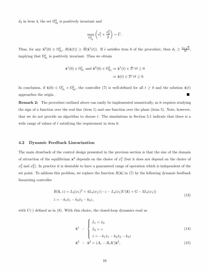
5.2 Dynamic Feedback Linearization

Following Procedure 2 we first need to choose U . To allow for a comparison with the Lyapunov-based

design, we set the same values of U and K as in Section 5.1. These yield the same horizontal operating

range Ω2d2

whose projection onto the (x3, x4) plane is depicted in Figure 7. Next, referring to item 3,

we need to fit an ellipsoid in D satisfying the invariance properties in item 3b. We plot the set D (see

Figure 9a) and choose the center of the ellipsoid to be at C = [1.70 · 10−2 0 0]>. We then need to find

scalars k1, k2, k3, a positive definite matrix H and a positive real number R such that, (1), A is Hurwitz,

(2), the ellipsoid N is contained in D and, (3), N is positively invariant when xd1 = C1 and, thus, when

b = 1/2HA[0 − C2 − C3]> = 0. When b = 0, checking positive invariance of N amounts to guaranteeing

that

S = 1/2(HA + A>H) (24)

23

0 0.005 0.01 0.015 0.02 0.025 0.03 0.035 0.04 0.045- 0.04

- 0.03

-0.02

- 0.01

0

0.01

0.02

0.03

0.04

0.05

0.06

x1

x2

x1

d

initial conditions(x

1(t),x

2(t))

Ω1d1

D

(a)

0 0.005 0.01 0.015 0.02 0.025 0.03 0.035 0.04 0.045-0.03

- 0.02

- 0.01

0

0.01

0.02

0.03

0.04

0.05

0.06

x1

x2

x1

d

initial conditions(x

1(t),x

2(t))

Ω1d1

D

(b)

Figure 8: Lyapunov control: Phase curves of the closed-loop system (9) for two different set points.

is negative semidefinite (see Lemma 2, part (iii)). As remarked earlier, (24) is a Lyapunov equation for A

which is guaranteed to have a solution, H, as long as A is Hurwitz. We can find H fulfilling the requirement

in item 3b as follows. Choose k1, k2, k3 so that A is Hurwitz, pick a negative definite matrix S and solve

the Lyapunov equation (24) to get a positive definite H. Next, choose R so that the associated ellipsoid

N is contained in D. Different choices of k1, k2, k3, and S yield different matrices H. By trial and error,

one can select H so that N approximates D to a reasonable degree. We choose k1 = 103, k2 = 1.11 · 103,

k3 = 111 and S = −diag[103, 103, 0.8]. These yield

H =

2.12 · 103 127.4 1

127.4 129.9 1

1 1 0.0164

.

Finally, choosing R = 0.12 we obtain N ⊂ D shown in Figure 9. The choice of parameters above guarantees

that, when xd1 = C1 = 1.70 · 10−2m, N is positively invariant. As pointed out in Remark 3, by varying xd

1

in a neighborhood of C1 and repeatedly checking the conditions in Lemma 2, one finds an interval I ⊂ R

such that ∀xd1 ∈ I, N is positively invariant. By so doing we find that

I = [0.0115m, 0.0225m]. (25)

In conclusion, for any xd1 ∈ I, the set N is the vertical operating range of the platen. Figure 9 displays few

phase curves of the closed-loop vertical dynamics when xd1 = 0.0120m, together with the set I.

24

0.010.015

0.020.025

0.03-0.05

0

0.05

-4

-3

-2

-1

0

1

2

3

4

5

x2

x1

z

Ix

1

d

initial conditions

phase curves

N

∂D

(a)

0.01 0.015 0.02 0.025

-0.04

-0.03

-0.02

-0.01

0

0.01

0.02

0.03

0.04

x1

x2

I

x1

d

initial conditions

phase curves

(b)

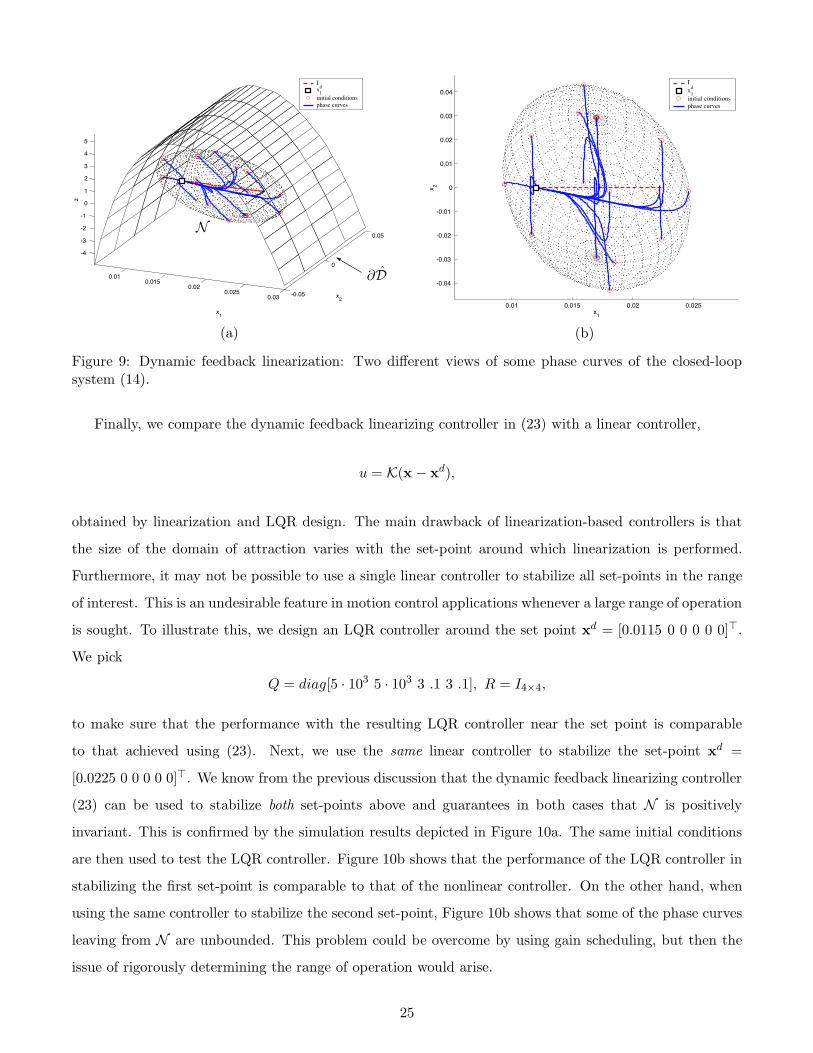
Figure 9: Dynamic feedback linearization: Two different views of some phase curves of the closed-loopsystem (14).

Finally, we compare the dynamic feedback linearizing controller in (23) with a linear controller,

u = K(x − xd),

obtained by linearization and LQR design. The main drawback of linearization-based controllers is that

the size of the domain of attraction varies with the set-point around which linearization is performed.

Furthermore, it may not be possible to use a single linear controller to stabilize all set-points in the range

of interest. This is an undesirable feature in motion control applications whenever a large range of operation

is sought. To illustrate this, we design an LQR controller around the set point xd = [0.0115 0 0 0 0 0]>.

We pick

Q = diag[5 · 103 5 · 103 3 .1 3 .1], R = I4×4,

to make sure that the performance with the resulting LQR controller near the set point is comparable

to that achieved using (23). Next, we use the same linear controller to stabilize the set-point xd =

[0.0225 0 0 0 0 0]>. We know from the previous discussion that the dynamic feedback linearizing controller

(23) can be used to stabilize both set-points above and guarantees in both cases that N is positively

invariant. This is confirmed by the simulation results depicted in Figure 10a. The same initial conditions

are then used to test the LQR controller. Figure 10b shows that the performance of the LQR controller in

stabilizing the first set-point is comparable to that of the nonlinear controller. On the other hand, when

using the same controller to stabilize the second set-point, Figure 10b shows that some of the phase curves

leaving from N are unbounded. This problem could be overcome by using gain scheduling, but then the

issue of rigorously determining the range of operation would arise.

25

0.01 0.015 0.02 0.025

-0.04

-0.03

-0.02

-0.01

0

0.01

0.02

0.03

0.04

x1

x2

I

x1

d

initial conditions

trajectories to 1st set point

trajectories to 2nd set point

(a)

0.01 0.015 0.02 0.025

-0.04

-0.03

-0.02

-0.01

0

0.01

0.02

0.03

0.04

x1

x2

Ix

1

d

initial conditions

trajectories to 1st set point

trajectories to 2nd set point

(b)

Figure 10: Phase curves of the closed-loop system with (a) nonlinear and (b) linear feedback approachingtwo different setpoints.

6 Conclusions

We have presented two nonlinear control strategies to regulate the position of the platen to a desired set

point. In both cases we have outlined a procedure to estimate the domain of attraction of the set point

which provides the guaranteed range of operation of the device. Our simulation results in Section 5 show

that both controllers do not restrict the horizontal range of operation.

On the other hand, air-gap control presents a greater challenge, making the estimation of the vertical

operating range crucial. The vertical operating range of the Lyapunov controller in Section 4.1 depends

on the choice of xd1 and gets smaller as (xd

1, 0) gets closer to the boundary of the set D (see Figure 8). This

is an undesirable feature of the controller in Section 4.1. The dynamic feedback linearizing controller in

Section 4.2 overcomes this problem because it allows one to find (through Procedure 2) an operating range

N which is valid for all choices of xd1 in an interval I which can be computed a priori (in our simulations

I = [0.0115m, 0.0225m]). A comparison between Figures 8 and 9b shows that the operating range of the

dynamic feedback linearizing controller is larger than that of the Lyapunov controller for both choices of

the set point in Figures 8a and 8b.

7 Aknowledgements

We are grateful to R. B. Owen for his useful comments and suggestions.

26

References

Gantmacher, F. R.: 1977, The Theory of Matrices, Chelsea Publishing Company, New York.

Gieras, J. F. and Piech, Z. J.: 2000, Linear Synchronous Motors: transportation and automation systems,

CRC Press, Boca Raton, FL, USA.

Kim, W. and Trumper, D.: 1998, High-precision levitation stage for photolithography, Precision Engineer-

ing 22, 66–67.

Nasar, S. and Xiong, G.: 1988, Determination of the field of a permanent-magnet disk machine using the

concept of magnetic charge, IEEE Transactions on Magnetics 24(3), 2038–2044.

Nasar, S. and Xiong, G.: 1989, Analysis of fields and forces in a permanent magnet linear synchronous

machine based on the concept of magnetic charge, IEEE Transactions on Magnetics 25(3), 2713–2719.

Shan, X., Kuo, S.-K., Zhang, J. and Menq, C.-H.: 2002, Ultra precision motion control of a multiple degrees

of freedom magnetic suspension stage, IEEE/ASME Transactions on Mechatronics 7(1), 67–78.

Tsai, K.-Y. and Yen, J.-Y.: 1999, Servo system design of a high-resolution piezo-driven fine stage for step-

and-repeat microlithography systems, The 25th Annual Conference of the IEEE Industrial Electonics

Society, Vol. 1, pp. 11–16.

Zhu, Z. and Howe, D.: 1993, Instantaneous magnetic field distribution in brushless permanent magnet DC

motors, part III: Effect of stator slotting, IEEE Transactions on Magnetics 29(1), 143–151.

27