mixed effects trees and forests for clustered data
TRANSCRIPT

HEC Montreal
Affiliee a l’universite de Montreal
Mixed Effects Trees and Forestsfor Clustered Data
PAR
AHLEM HAJJEM
THESE
presentee en vue de l’obtention du grade
de Philosophiæ Doctor (Ph.D.) en administration
Specialisation : Methodes Quantitatives
SEPTEMBRE 2010
c© Ahlem HAJJEM, 2010

HEC Montreal
Affiliee a l’universite de Montreal
Cette these est intitulee :
Mixed Effects Trees and Forestsfor Clustered Data
Presentee par Ahlem Hajjem
a ete evaluee par un jury compose des personnes suivantes:
Marc Fredette..........................................................
President rapporteur
Francois Bellavance..........................................................
Co-directeur de recherche
Denis Larocque..........................................................
Co-directeur de recherche
Cataldo Zuccaro..........................................................
Membre du jury
Thierry Duchesne..........................................................
Examinateur externe
Raf Jans..........................................................
Representant du doyen de la FES

ii
RESUME
Les methodes d’arbres, qui sont des outils populaires et apprecies d’analyse et d’exploi-
tation de donnees, etaient a l’origine developpees sous l’hypothese de donnees independantes.
Les travaux anterieurs qui ont adapte ces methodes aux donnees correlees sont bases sur l’ap-
proche multivariee des mesures repetees. L’objectif principal de cette these est d’adapter la
methode d’arbre standard aux donnees correlees du fait de leur structure hierarchique. Pour
cela, nous avons suivi une approche par les effets mixtes. Cette approche est plus flexible
en ce qui concerne les donnees puisque les observations correlees sont percues comme etant
imbriquees a l’interieur des groupes et non pas comme des vecteurs de reponses multiples.
Cette these est composee de trois articles. Dans le premier article, nous procedons
a une extension de la methode d’arbre de regression standard aux donnees hierarchiques
avec une variable de reponse continue. Nous proposons alors une methode d’arbre nommee
“mixed effects regression tree” (MERT). Dans le second article, nous procedons a une ex-
tension de la methodologie MERT a d’autres types de reponses (reponses binaires, donnees
de comptage, reponses categorielles ordonnees, reponses multicategorielles nominales). Pour
cela, nous proposons une methode d’arbre nommee “generalized mixed effects regression
tree” (GMERT). Nous proposons dans le troisieme article la methode de foret aleatoire a
effets mixtes, nommee “mixed effects random forest” (MERF).
Les resultats des etudes de simulations menees dans les trois articles montrent qu’en
presence de correlation intra-groupe, les nouvelles methodes d’arbres sont preferables a celles
supposant l’independance des donnees.
Mots cles : Methodes d’arbres, foret aleatoire, donnees hierarchiques, effets mixtes,
algorithme d’esperance-maximisation (EM), quasi-vraisemblance penalisee (PQL).

iii
ABSTRACT
Tree based methods, which are very popular and appreciated data analysis tools, were
firstly developed under the assumption of independent data. Previous works adapting them
to correlated data are based on the multivariate repeated-measures approach. The main
goal of this thesis is to extend standard tree methods to clustered and hence correlated
data, using the mixed effects approach. This approach is more flexible in terms of data
requirements because the correlated observations are viewed as nested within clusters rather
than as vectors of multivariate repeated responses.
This thesis is composed of three articles. In the first paper, we propose the “mixed
effects regression tree” (MERT) method. It is an extension of the standard regression tree
method to the case of clustered data with continuously measured outcome. The second
paper presents the generalized mixed effects regression tree (GMERT) method, which is an
extension of MERT methodology to other types of outcomes (binary outcomes, counts data,
ordered categorical outcomes, and multicategory nominal scale outcomes). We propose in
the third paper the “mixed effects random forest” (MERF) method, which is an extension of
the standard random forest method to the case of clustered data with continuously measured
outcome.
The results of the simulations studies conducted in the three papers show that, when
cluster-correlation is present, the new tree methods are preferable over the standard ones
assuming independence of the data.
Keywords : Tree based methods, random forest, clustered data, mixed effects, expectation-
maximization (EM) algorithm, penalized quasi-likelihood (PQL) algorithm.

iv
TABLE DES MATIERES
RESUME . . . . . . . . . . . . . . . . . . . . . . . . . . . . . . . . . . . . . . . . . . . . . . . ii
ABSTRACT . . . . . . . . . . . . . . . . . . . . . . . . . . . . . . . . . . . . . . . . . . . . . iii
LISTE DES TABLEAUX . . . . . . . . . . . . . . . . . . . . . . . . . . . . . . . . . . . . . . vi
LISTE DES FIGURES . . . . . . . . . . . . . . . . . . . . . . . . . . . . . . . . . . . . . . . vii
INTRODUCTION GENERALE . . . . . . . . . . . . . . . . . . . . . . . . . . . . . . . . . . 1
ARTICLE IMIXED EFFECTS REGRESSION TREES FOR CLUSTERED DATA . . . . . . . . . . . . 4
1.1 Abstract . . . . . . . . . . . . . . . . . . . . . . . . . . . . . . . . . . . . . . . . . . . . . 5
1.2 Introduction . . . . . . . . . . . . . . . . . . . . . . . . . . . . . . . . . . . . . . . . . . . 5
1.3 Mixed Effects Regression Tree Approach . . . . . . . . . . . . . . . . . . . . . . . . . . . 7
1.3.1 EM Algorithm for the Linear Mixed Effects Model . . . . . . . . . . . . . . . . . 7
1.3.2 EM Algorithm for the Mixed Effects Regression Trees . . . . . . . . . . . . . . . 9
1.4 Simulation . . . . . . . . . . . . . . . . . . . . . . . . . . . . . . . . . . . . . . . . . . . . 12
1.4.1 Simulation Design . . . . . . . . . . . . . . . . . . . . . . . . . . . . . . . . . . . 13
1.4.2 Simulation Results . . . . . . . . . . . . . . . . . . . . . . . . . . . . . . . . . . . 15
1.5 Data Example . . . . . . . . . . . . . . . . . . . . . . . . . . . . . . . . . . . . . . . . . 17
1.5.1 Description of Observation and Cluster Level Covariates . . . . . . . . . . . . . . 18
1.5.2 Results . . . . . . . . . . . . . . . . . . . . . . . . . . . . . . . . . . . . . . . . . 19
1.6 Discussion . . . . . . . . . . . . . . . . . . . . . . . . . . . . . . . . . . . . . . . . . . . . 20
1.7 Conclusion . . . . . . . . . . . . . . . . . . . . . . . . . . . . . . . . . . . . . . . . . . . 22
1.8 References . . . . . . . . . . . . . . . . . . . . . . . . . . . . . . . . . . . . . . . . . . . . 24
ARTICLE IIGENERALIZED MIXED EFFECTS REGRESSION TREES . . . . . . . . . . . . . . . . . 34
2.1 Abstract . . . . . . . . . . . . . . . . . . . . . . . . . . . . . . . . . . . . . . . . . . . . . 35
2.2 Introduction . . . . . . . . . . . . . . . . . . . . . . . . . . . . . . . . . . . . . . . . . . . 35
2.3 Generalized Mixed Effects Regression Tree . . . . . . . . . . . . . . . . . . . . . . . . . . 37
2.3.1 PQL Algorithm for the Generalized Linear Mixed Models . . . . . . . . . . . . . 37
2.3.2 PQL Algorithm for the Generalized Mixed Effects Regression Trees . . . . . . . 40
2.3.3 GMERT Model in the Binary Response Case . . . . . . . . . . . . . . . . . . . . 43
2.4 Simulation . . . . . . . . . . . . . . . . . . . . . . . . . . . . . . . . . . . . . . . . . . . . 44

v
2.4.1 Simulation Design . . . . . . . . . . . . . . . . . . . . . . . . . . . . . . . . . . . 45
2.4.2 Simulation Results . . . . . . . . . . . . . . . . . . . . . . . . . . . . . . . . . . . 47
2.5 Discussion . . . . . . . . . . . . . . . . . . . . . . . . . . . . . . . . . . . . . . . . . . . . 50
2.6 Conclusion . . . . . . . . . . . . . . . . . . . . . . . . . . . . . . . . . . . . . . . . . . . 50
2.7 Appendix : Weighted Standard Regression Tree Within GMERT Algorithm . . . . . . . 52
2.8 References . . . . . . . . . . . . . . . . . . . . . . . . . . . . . . . . . . . . . . . . . . . . 53
ARTICLE IIIMIXED EFFECTS RANDOM FOREST FOR CLUSTERED DATA . . . . . . . . . . . . . 58
3.1 Abstract . . . . . . . . . . . . . . . . . . . . . . . . . . . . . . . . . . . . . . . . . . . . . 59
3.2 Introduction . . . . . . . . . . . . . . . . . . . . . . . . . . . . . . . . . . . . . . . . . . . 59
3.3 Mixed Effects Random Forest Approach . . . . . . . . . . . . . . . . . . . . . . . . . . . 60
3.4 Simulation . . . . . . . . . . . . . . . . . . . . . . . . . . . . . . . . . . . . . . . . . . . . 62
3.4.1 Simulation Design . . . . . . . . . . . . . . . . . . . . . . . . . . . . . . . . . . . 63
3.4.2 Simulation Results . . . . . . . . . . . . . . . . . . . . . . . . . . . . . . . . . . . 65
3.5 Concluding Remarks . . . . . . . . . . . . . . . . . . . . . . . . . . . . . . . . . . . . . . 68
3.6 References . . . . . . . . . . . . . . . . . . . . . . . . . . . . . . . . . . . . . . . . . . . . 70
CONCLUSION GENERALE . . . . . . . . . . . . . . . . . . . . . . . . . . . . . . . . . . . . 78
BIBLIOGRAPHIE . . . . . . . . . . . . . . . . . . . . . . . . . . . . . . . . . . . . . . . . . . 81
vi
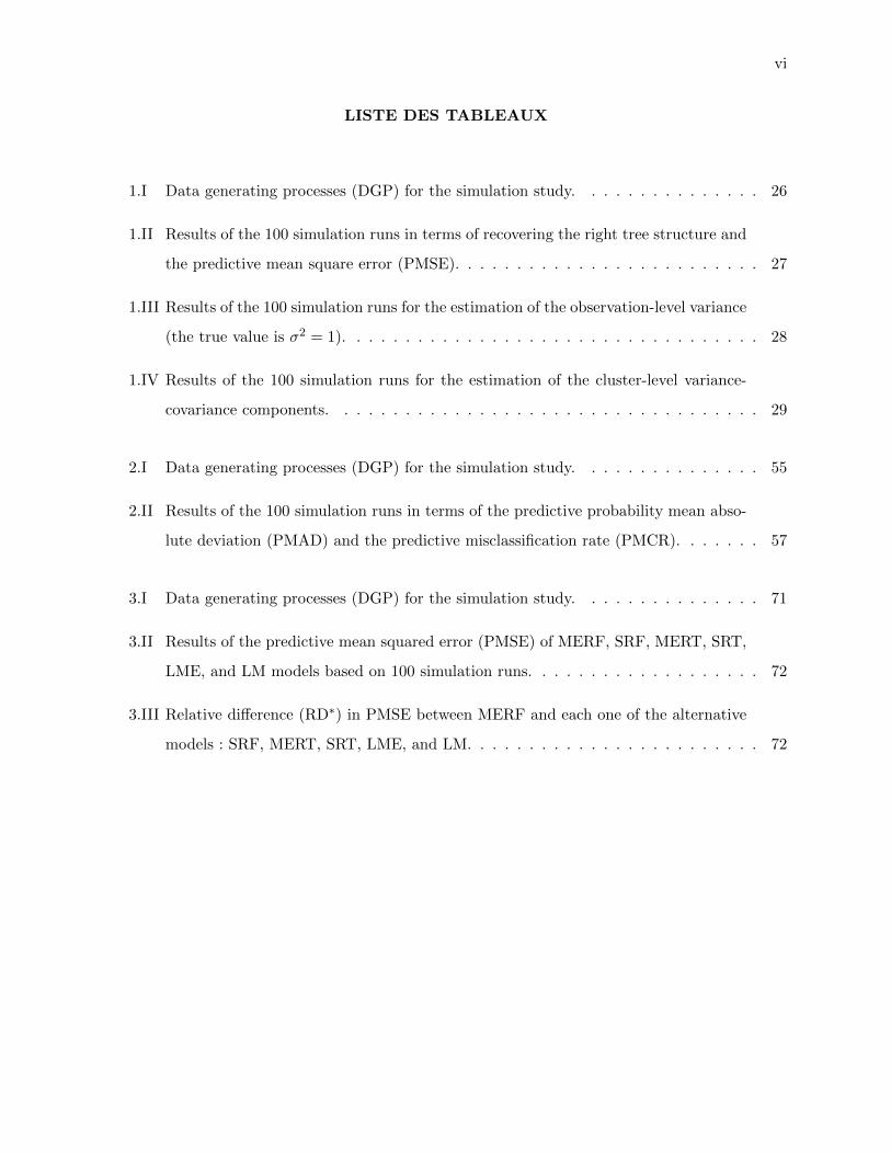
LISTE DES TABLEAUX
1.I Data generating processes (DGP) for the simulation study. . . . . . . . . . . . . . . 26
1.II Results of the 100 simulation runs in terms of recovering the right tree structure and
the predictive mean square error (PMSE). . . . . . . . . . . . . . . . . . . . . . . . . 27
1.III Results of the 100 simulation runs for the estimation of the observation-level variance
(the true value is σ2 = 1). . . . . . . . . . . . . . . . . . . . . . . . . . . . . . . . . . 28
1.IV Results of the 100 simulation runs for the estimation of the cluster-level variance-
covariance components. . . . . . . . . . . . . . . . . . . . . . . . . . . . . . . . . . . 29
2.I Data generating processes (DGP) for the simulation study. . . . . . . . . . . . . . . 55
2.II Results of the 100 simulation runs in terms of the predictive probability mean abso-
lute deviation (PMAD) and the predictive misclassification rate (PMCR). . . . . . . 57
3.I Data generating processes (DGP) for the simulation study. . . . . . . . . . . . . . . 71
3.II Results of the predictive mean squared error (PMSE) of MERF, SRF, MERT, SRT,
LME, and LM models based on 100 simulation runs. . . . . . . . . . . . . . . . . . . 72
3.III Relative difference (RD∗) in PMSE between MERF and each one of the alternative
models : SRF, MERT, SRT, LME, and LM. . . . . . . . . . . . . . . . . . . . . . . . 72

vii
LISTE DES FIGURES
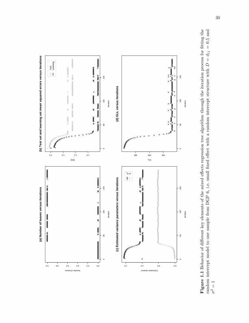
1.1 Behavior of different key elements of the mixed effects regression tree algorithm
through the iteration process for fitting the random intercept model to one sample
from DGP 6, i.e. small fixed effect with a random intercept structure with D = d11 =
0.5 and σ2 = 1 . . . . . . . . . . . . . . . . . . . . . . . . . . . . . . . . . . . . . . . 30
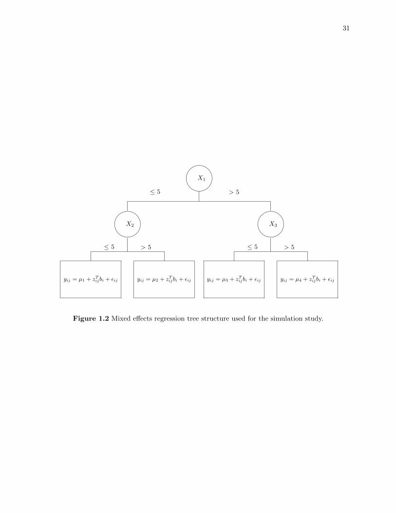
1.2 Mixed effects regression tree structure used for the simulation study. . . . . . . . . . 31
1.3 The first three levels of the standard regression tree for the data example on first-
week box office revenues (on the log scale). When the condition below a node is true
then go to the left node, otherwise go to the right node. The complete tree has 44
leaves. . . . . . . . . . . . . . . . . . . . . . . . . . . . . . . . . . . . . . . . . . . . . 32
1.4 The first three levels of the random intercept regression tree for the data example on
first-week box office revenues (on the log scale). When the condition below a node is
true then go to the left node, otherwise go to the right node. The complete tree has
28 leaves. . . . . . . . . . . . . . . . . . . . . . . . . . . . . . . . . . . . . . . . . . . 33
2.1 Generalized mixed effects tree structure used for the simulation study, with g(.) being
the logit link function and g(.)−1 the inverse-logit or logistic function. . . . . . . . . 56
3.1 Distribution over the 100 simulation runs of the relative difference in PMSE between
MERF and SRF . . . . . . . . . . . . . . . . . . . . . . . . . . . . . . . . . . . . . . 73
3.2 Distribution over the 100 simulation runs of the relative difference in PMSE between
MERF and MERT . . . . . . . . . . . . . . . . . . . . . . . . . . . . . . . . . . . . . 74
3.3 Distribution over the 100 simulation runs of the relative difference in PMSE between
MERF and SRT . . . . . . . . . . . . . . . . . . . . . . . . . . . . . . . . . . . . . . 75
3.4 Distribution over the 100 simulation runs of the relative difference in PMSE between
MERF and LME . . . . . . . . . . . . . . . . . . . . . . . . . . . . . . . . . . . . . . 76

viii
3.5 Distribution over the 100 simulation runs of the relative difference in PMSE between
MERF and LM . . . . . . . . . . . . . . . . . . . . . . . . . . . . . . . . . . . . . . . 77

ix
REMERCIEMENTS
Je remercie Dieu pour m’avoir donne la volonte et la patience pour accomplir ce travail.
Un grand merci a ma famille pour son soutien et encouragement.
Je voudrais aussi exprimer toute ma gratitude envers mes co-directeurs, Professeur Francois
Bellavance et Professeur Denis Larocque, pour leur grande disponibilite, leur implication, et leurs
conseils precieux.
Je remercie aussi tous les membres du jury pour avoir accepte de lire et commenter ce travail.
Mes remerciements s’adressent egalement a HEC Montreal, au Conseil de Recherche en
Sciences Naturelles et en Genie du Canada (CRSNG), et au Fonds Quebecois de la Recherche
sur la Nature et les Technologies (FQRNT), pour leur support financier.
Merci infiniment !

INTRODUCTION GENERALE
Les methodes d’arbres sont des techniques traditionnelles d’analyse et d’exploitation de
donnees. Elles sont devenues populaires grace a l’algorithme CART (classification and regression
trees) de Breiman et al. (1984). Comparativement aux modeles de regression parametriques, ces
methodes ont plusieurs avantages : Elles peuvent analyser facilement des grandes bases de donnees
comprenant un nombre eleve de covariables, elles peuvent detecter de facon automatique les in-
teractions potentielles entre ces dernieres, et elles sont robustes face aux problemes d’observations
extremes et de colinearite.
Les methodes d’arbres supposent l’independance des donnees. Or, cette hypothese n’est cer-
tainement pas satisfaite dans le cas de donnees hierarchiques. Ces dernieres sont souvent obtenues
par un echantillonnage multiniveaux, ou les observations sont imbriquees a l’interieur d’unites de
niveau superieur (groupes). Elles sont communement presentes dans plusieurs champs de recherche
(e.g., Raudenbush and Bryk, 2002 ; Goldstein, 2003 ; Fitzmaurice, Laird, and Ware, 2004). La
structure hierarchique de ces donnees implique que les observations provenant d’un meme groupe
sont souvent plus similaires entre elles que les observations provenant de groupes differents. Sou-
vent, ces donnees comprennent deux types de covariables, celles decrivant l’observation au niveau
hierarchique inferieur et celles decrivant le groupe, et incluent deux sources de variations, intra- et
inter- groupes. Des effets fixes mais aussi aleatoires servent a expliquer, au moins partiellement, ces
deux sources de variabilite.
L’objectif principal de cette these est d’adapter les methodes d’arbres standards aux donnees
hierarchiques, et ce en suivant une approche par les effets mixtes (fixes et aleatoires). Les travaux
anterieurs (Segal, 1992 ; Zhang, 1998 ; Abdolell, Leblanc, Stephens, and Harrison, 2002 ; Lee, 2005)
qui ont etendu les methodes d’arbres dans le but d’accommoder la dependance des donnees sont
bases sur l’approche multivariee des mesures repetees. L’approche par les effets mixtes est plus
flexible en termes de donnees parce que les observations correlees sont percues comme etant im-
briquees a l’interieur des groupes plutot que comme des vecteurs de reponses multiples. Il y a un
avantage a suivre cette approche puisqu’elle permet : 1) d’analyser des donnees ou les groupes

2
sont de tailles inegales, 2) de considerer les covariables du niveau observation dans le processus
d’embranchement, ce qui permet de separer les observations provenant d’un meme groupe dans des
noeuds differents, et 3) d’inclure des effets aleatoires.
Trois articles font l’objet de cette these. Dans le premier article, nous proposons une exten-
sion des methodes d’arbres standards aux donnees hierarchiques avec une variable reponse conti-
nue. Nous avons nomme cette extension “mixed effects regression tree” (MERT). Nous l’avons
implemente en utilisant un algorithme d’arbre standard a l’interieur du cadre bien connu de l’al-
gorithme “esperance-maximisation” (EM). Nous l’avons aussi illustre en analysant des donnees sur
les revenus du box-office de la premiere semaine des films presentes dans la province de Quebec au
Canada sur la periode allant de 2001 a 2008. Les resultats de la simulation montrent que la perfor-
mance predictive de MERT est meilleure que celle de l’arbre de regression standard, en particulier
lorsque les effets aleatoires sont importants.
Dans le deuxieme article, nous proposons une extension de la methodologie d’arbre de
regression a effets mixtes (MERT), qui est concue pour une reponse continue, a d’autres types de
reponses (reponses binaires, donnees de comptage, reponses categorielles ordonnees, reponses mul-
ticategorielles nominales). Nous avons nomme cette extension “generalized mixed effects regression
tree” (GMERT). Cette methode utilise la quasi-vraisemblance penalisee (PQL) pour l’estimation et
l’algorithme esperance-maximisation (EM) pour la computation. Les resultats de l’etude de simu-
lation menee pour le cas de reponse binaire montrent qu’en presence d’effets aleatoires la methode
GMERT a une performance predictive nettement meilleure que celle de l’arbre de classification
standard.
Par ailleurs, la performance predictive d’un seul arbre peut souvent etre amelioree au depend
de l’interpretabilite en utilisant un ensemble d’arbres. Le bagging et la foret aleatoire en general
(Breiman, 1996, 2001) sont des methodes ensemblistes tres connues et tres puissantes dans le cas
des arbres. Sur la base des conclusions des deux premiers articles, il est devenu clair que l’appli-
cation directe de l’algorithme standard de foret aleatoire aux donnees hierarchiques impliquerait
necessairement une performance predictive moins qu’optimale de la part de chaque arbre individuel
a l’interieur de la foret. Ainsi, nous proposons dans le troisieme article une methode de foret aleatoire
a effets mixtes. Nous avons nommee cette methode “mixed effects random forest” (MERF). Il s’agit
d’une extension de la methode standard de foret aleatoire aux donnees hierarchiques avec une

3
reponse continue. Nous l’avons implementee en utilisant un algorithme standard de foret aleatoire
a l’interieur de l’algorithme EM. Les resultats de la simulation menee dans cet article sont promet-
teurs et montrent que le gain sur le plan predictif suite a l’utilisation de MERF a la place de la
foret standard augmente en fonction de l’importance des effets aleatoires.

ARTICLE I
MIXED EFFECTS REGRESSION TREES FOR CLUSTERED DATA
Ahlem Hajjem, Francois Bellavance and Denis Larocque
...
Department of Management Sciences
HEC Montreal, 3000, chemin de la Cote-Sainte-Catherine,
Montreal, QC, Canada H3T 2A7

5
1.1 Abstract
This paper presents an extension of the standard regression tree method to clustered data. Previous
works extending tree methods to accommodate correlated data are mainly based on the multivariate repeated-
measures approach. We propose a “mixed effects regression tree” method where the correlated observations
are viewed as nested within clusters rather than as vectors of multivariate repeated responses. The proposed
method can handle unbalanced clusters, allows observations within clusters to be splitted, and can incorporate
random effects and observation-level covariates. We implemented the proposed method using a standard tree
algorithm within the framework of the expectation-maximization (EM) algorithm. The simulation results
show that the proposed regression tree method provide substantial improvements over standard trees when
the random effects are non negligible. A real data example illustrates the proposed method.
Keywords : Tree based methods, clustered data, mixed effects, expectation-maximization (EM)
algorithm.
1.2 Introduction
Clustered data, often obtained by multistage sampling with observations nested within
higher-level units (clusters), is common throughout many areas of research (e.g., Raudenbush
and Bryk, 2002 ; Goldstein, 2003 ; Fitzmaurice, Laird, and Ware, 2004). The data structure
consists of individuals nested within groups. These data may include two types of covariates,
observation-level and cluster-level covariates, and involve two sources of variation, within
and between clusters. Usually, observations that belong to the same cluster tend to be more
similar to each other than observations from different clusters. The focus of this paper is
to extend the standard regression tree methods to clustered data and therefore take into
account the correlation between observations within a cluster.
Tree based methods became popular with the CART (classification and regression
trees) paradigm (Breiman, Friedman, Olshen, and Stone, 1984). They provide many advan-
tages compared to parametric models : They can handle large data sets with many covariates,
they are robust to outliers and collinearity problems, and they detect automatically potential
interactions between covariates.

6
If a standard tree algorithm is directly applied to clustered data, any tree node could
include observations belonging to different clusters, and the question of which summary
response value should be attached to them arises, i.e. overall average response or cluster-
specific average response within each node. Furthermore, the inclusion of the observation-
level and cluster-level covariates as candidates in the splitting process is not always enough
to ensure that the nested structure of the data is fully taken into account. Not considering
the clustered aspect of the data in the splitting process constitutes an evident loss of likely
valuable information. To that end, statistical models to analyze clustered data often imply
an additional random-effect component in addition to the fixed-effect component. The larger
the random effects, the harder it will be for a standard tree algorithm to find the right tree
structure, which should affect negatively the prediction accuracy. This will be illustrated in
the simulation study in Section 1.4.
To legitimize the application of standard tree methodology to clustered data, one could
remove the random or cluster-specific component, and then apply a standard tree algorithm,
such as CART, only to the fixed or population-averaged component. This constitutes the
key point of the regression tree approach presented in this paper, named “mixed effects
regression tree”. It is an extension of standard regression trees to clustered data that can
appropriately deal with random effects.
The proposed mixed effects regression tree method have the following characteristics :
1. It can handle clusters with different numbers of observations (unbalanced clusters).
2. It allows the inclusion of observation-level and cluster-level covariates in the splitting
process, and consequently, observations from the same cluster can be separated into
different nodes during the tree growing process.
3. It allows observation-level covariates to have random effects.
Previous extensions of tree based methods to accommodate the correlation structure
induced by clustered data were developed for longitudinal settings (e.g., Segal, 1992 ; Zhang,
1998 ; Yu and Lambert, 1999 ; Abdolell, Leblanc, Stephens, and Harrison, 2002 ; Lee, 2005 ;
Ghattas and Nerini, 2007). These extensions do not allow observations within a cluster (i.e.

7
repeated observations over time for a given subject) to be splitted into different nodes.
This paper presents and evaluates an extension of regression trees for clustered data.
The remainder of this article is organized as follows : Section 1.3 describes the proposed
mixed effects regression tree approach ; Section 1.4 presents a simulation study to evaluate
the performance of the method ; Section 1.5 illustrates the application of the method with a
real data set ; Section 1.6 discusses a number of related issues.
1.3 Mixed Effects Regression Tree Approach
Statistical model for clustered data typically include two components : A fixed or
population-averaged and a random or cluster-specific component. The basic idea behind the
proposed mixed effects regression tree is to dissociate the fixed from the random effects. We
use a standard regression tree to model the fixed effects and a node-invariant linear structure
at each terminal node of the tree to model the random effects. The method is implemen-
ted using a standard tree algorithm within the framework of the expectation-maximization
(EM) algorithm (Dempster, Laird, and Rubin, 1977 ; McLachlan and Krishnan, 1997). More
precisely, the linear estimation of the fixed component in the linear mixed effects (LME)
model (Harville, 1976, 1977 ; Laird and Ware, 1982) is replaced by a standard regression tree
algorithm. Let’s first briefly review the LME model and the EM algorithm.
1.3.1 EM Algorithm for the Linear Mixed Effects Model
The LME model is generally written in the following form :
yi = Xiβ + Zibi + εi,
bi ∼ Nq(0, D), εi ∼ Nni(0, Ri), (1.1)
i = 1, ..., n,
where yi = [yi1, ..., yini ]T is the ni× 1 vector of responses for the ni observations in cluster i,
Xi = [xi1, ..., xini ]T is the ni × p matrix of fixed-effects covariates, Zi = [zi1, ..., zini ]
T is the

8
ni × q matrix of random-effects covariates, εi = [εi1, ..., εini ]T is the ni × 1 vector of errors,
bi = (bi1, ..., biq)T is the q × 1 unknown vector of random effects for cluster i, and β is the
p× 1 unknown vector of parameters for the fixed effects. The total number of observations
is N =∑n
i=1 ni. The covariance matrix of bi is D while Ri is the covariance matrix of εi.
The usual LME model also assumes that bi and εi are independent and normally distributed
and that the between-clusters observations are independent. Hence, the covariance matrix of
the vector of observations yi in cluster i is Vi = Cov(yi) = ZiDZTi +Ri, and V = Cov(y) =
diag(V1, . . . , Vn), where y = [yT1 , ..., yTn ]T . We will further assume that the correlation is
induced solely via the between-clusters variation, that is, Ri is diagonal (Ri = σ2Ini , i =
1, ..., n). This assumption is suitable for a large class of clustered data problems (Raudenbush
and Bryk, 2002, page 30).
The parameters in LME models can be estimated by the method of maximum likeli-
hood (ML) implemented with the EM algorithm. This algorithm addresses the problem of
maximizing the likelihood by considering it like a missing data problem. More precisely, the
yi are the observed data and the bi are the missing data. Thus, the complete data are (yi, bi),
i = 1, ..., n, while β, σ2, and D are the parameters to be estimated. The general technique
is to calculate the expected values of the missing objects, given current parameter estimates
(expectation step), and then to use those expected values to update the parameter estimates
(maximization step). These two steps are repeated until convergence.
The major cycle for the ML-based EM-algorithm, as described in §2.2.5 of Wu and
Zhang (2006), is as follows :
Step 0. Set r = 0. Let σ2(0) = 1, and D(0) = Iq.
Step 1. Set r = r + 1. Update β(r) and bi(r)
β(r) =
(n∑i=1
XTi V
−1i(r−1)Xi
)−1( n∑i=1
XTi V
−1i(r−1)yi
),
bi(r) = D(r−1)ZTi V−1i(r−1)
(yi −Xiβ(r)
), i = 1, ..., n,
where Vi(r−1) = ZiD(r−1)ZTi + σ2
(r−1)Ini , i = 1, ..., n.

9
Step 2. Update σ2(r), and D(r) using
σ2(r) = N−1
n∑i=1
{εTi(r)εi(r) + σ2
(r−1)[ni − σ2(r−1)trace(Vi(r−1))]
},
D(r) = n−1
n∑i=1
{bi(r)b
Ti(r) + [D(r−1) − D(r−1)Z
Ti V−1i(r−1)ZiD(r−1)]
},
where εi(r) = yi −Xiβ(r) − Zibi(r), N =∑n
i=1 ni.
Step 3. Repeat steps 1 and 2 until convergence.
1.3.2 EM Algorithm for the Mixed Effects Regression Trees
The proposed mixed effects regression tree model is :
yi = f(Xi) + Zibi + εi,
bi ∼ Nq(0, D), εi ∼ Nni(0, Ri), (1.2)
i = 1, ..., n,
where all quantities are defined as in Section 1.3.1 except that the linear fixed part Xiβ in
(1.1) is replaced by the function f(Xi) that will be estimated with a standard tree based
model. The random part, Zibi, is still assumed linear.
The mixed effects tree algorithm is the ML-based EM-algorithm in which we replace
the linear structure used to estimate the fixed part of the model by a standard tree structure.
The algorithm is as follows :
Step 0. Set r = 0. Let bi(0) = 0, σ2(0) = 1, and D(0) = Iq.
Step 1. Set r = r + 1. Update y∗i(r), f(Xi)(r), and bi(r)
i) y∗i(r) = yi − Zibi(r−1), i = 1, ..., n,
ii) Let f(Xi)(r) be an estimate of f(Xi) obtained from a standard tree algorithm with
y∗i(r) as responses and Xi, i = 1, . . . , n, as covariates. Note that the tree is built

10
as usual using all N individual observations as inputs along with their covariate
vectors,
iii) bi(r) = D(r−1)ZTi V−1i(r−1)
(yi − f(Xi)(r)
), i = 1, ..., n,
where Vi(r−1) = ZiD(r−1)ZTi + σ2
(r−1)Ini , i = 1, ..., n.
Step 2. Update σ2(r), and D(r) using
σ2(r) = N−1
n∑i=1
{εTi(r)εi(r) + σ2
(r−1)[ni − σ2(r−1)trace(Vi(r−1))]
}D(r) = n−1
n∑i=1
{bi(r)b
Ti(r) + [D(r−1) − D(r−1)Z
Ti V−1i(r−1)ZiD(r−1)]
},
where εi(r) = yi − f(Xi)(r) − Zibi(r).
Step 3. Repeat steps 1 and 2 until convergence.
In words, the algorithm starts at step 0 with default values for bi, σ2, and D. At step
1, it first calculates the fixed part of the response variable, y∗i , i.e., the response variable
from which we remove the current available value of the random part. Second, it estimates
the fixed component f(Xi) using a standard tree algorithm with y∗i as responses and Xi as
covariates. Third, it updates bi. At step 2, it updates the variance components σ2 and D
based on the residuals after the estimated fixed component f(Xi) is removed from the raw
data yi It keeps iterating by repeating steps 1 and 2 until convergence.
The convergence of the algorithm is monitored by computing, at each iteration, the
following generalized log-likelihood (GLL) criterion :
GLL(f, bi|y) =n∑i=1
{[yi − f(Xi)− Zibi]TR−1i [yi − f(Xi)− Zibi]
+ bTi D−1bi + log |D|+ log |Ri|}.
(1.3)
At each iteration, a single large tree is built and a subtree is selected using a pruning and
cross-validation method. Doing so introduces instability over the iteration process. Indeed,
a small change in the updated data (i.e., y∗i(r)) could produce a selected subtree with a

11
different number of leaves (terminal nodes). In order to give insight about the behavior of
GLL, Figure 1.1 shows the iteration process for one data set in one simulation run from the
simulation study described in more details in the next section. The GLL decreases sharply
at the beginning and stabilizes around iteration 40, but its value jumps once in a while from
iteration 50 to 200 (Figure 1.1d). These jumps occur when there is a change in the number
of leaves of the tree (Figure 1.1a). We also observe these jumps in the estimated variance
parameters (Figure 1.1c) and in the mean squared errors (Figure 1.1b). This is mainly due
to the instability associated with the choice of a single subtree at each iteration. All subtree
structures in this simulation run are exactly the same except that those with only three
terminal nodes do not have the split on the variable X2 (see Figure 1.1).
—————————-
Insert Figure 1.1 about here
—————————-
In practice, we suggest the following method to stop the iteration process and select a
final subtree model. First, we impose a minimum number of iterations to avoid early stopping
(e.g. 50), then we keep iterating until the absolute change in GLL is less than a given small
value (e.g. 1E-06). Once the stopping criterion is reached, we let the process continue for
an additional pre-determined number of iterations (e.g. 50 in Figure 1.1). We then find the
most frequent (modal value) number of leaves for the selected subtrees in the sequence of
additional iterations. The final subtree model chosen is the one corresponding to the last
iteration where the number of leaves is equal to the modal value. In the example presented
in Figure 1.1, the subtree model selected is the one in the very last iteration, a tree with
four leaves since it is the most frequent number of leaves in the 50 additional iterations after
the GLL stabilizes.
This algorithm is similar in terms of computational complexity to bagged trees (Brei-
man, 1996). While the latter uses bootstrap replicates of the learning data set, the proposed

12
algorithm iteratively computes updated data sets in terms of the response variable (i.e., y∗i(r)).
Both algorithms fit a standard regression tree to each one of the modified data sets. This
process entails no additional challenge in terms of computational complexity if it uses one of
the available and efficient implementation of a standard regression tree algorithm. Updating
the learning data set at each iteration in the proposed algorithm for mixed effects regression
trees is not too demanding since we have closed form expressions for the estimators of the
random effects bi and of the variance components σ2 and D. Note however that the number of
bootstrap samples is arbitrarily fixed in advance in the bagging algorithm, while the number
of iterations depends on the speed of convergence of the proposed EM algorithm for mixed
effects regression trees. Many factors may affect this convergence (e.g. : sample size, initial
values, instability of standard regression trees). The main disadvantage of the EM algorithm
is that it may require a large number of iterations before reaching the stopping criteria.
To predict the response for a new observation that belongs to a cluster among those
used to fit the mixed effects regression model, we use both its corresponding population-
averaged tree prediction and the predicted random part corresponding to its cluster. For a
new observation that belongs to a cluster not included in the sample used to estimate the
model parameters, we can only take the corresponding population-averaged tree prediction.
There exist a number of other nonlinear or nonparametric methods to model the fixed
part f(Xi) and/or the random part Zibi in (1.2) (e.g., Davidian and Giltinan, 1995 ; Zhang
and Davidian, 2004 ; Zhang, 1997 ; Wu and Zhang, 2006). These alternatives may be more
suitable in some applications. Tree methods are however attractive because they propose
easily interpretable models and are able, through their automatic detection of possible signi-
ficant interactions between covariates, to represent complex relationships.
1.4 Simulation
In this section, we investigate the performance of the mixed effects regression trees
in comparison to standard trees. The proposed method was implemented in R (R Deve-
lopment Core Team, 2007) using the function rpart (Therneau and Atkinson, 1997). This

13
function implements cost-complexity pruning based on cross-validation after an initial large
tree is grown. The default settings of rpart are used ; the largest tree is grown and pruned
automatically using the 1-SE rule of Breiman and al. (1984).
Within the mixed tree approach, we force the first 50 iterations, then we keep iterating
while the absolute change in GLL is not less than 1E-06 or we reach a maximum of 1000
iterations. Once the stopping criterion is met, we run an additional 50 iterations. The mixed
tree model chosen is the one corresponding to the last iteration where the number of leaves
is equal to the modal value over the last 50 mixed tree models.
To compare the performance of the standard and mixed effects regression tree methods,
we evaluate both their ability to find the true tree structure used to generate the data,
and their predictive accuracy measured by the predictive mean squared error (PMSE). In
addition, we look at how well are estimated the variance-covariance components at the
observation-level (σ2) and at the cluster-level (D) with the mixed effects regression tree
approach.
1.4.1 Simulation Design
The simulation design used has a hierarchical structure of 100 clusters with 55 obser-
vations generated in each cluster. The first five observations in each cluster form the training
sample, and the other 50 observations are left for the test sample. Consequently, the trees
are built with 500 observations (100 clusters of 5 observations). Three random variables, X1,
X2, and X3, are first generated independently with a uniform distribution in the interval
[0, 10] ; they serve as predictors. The response variable y is generated based on the following
fixed tree rules along with the random components :
Leaf 1. If x1ij ≤ 5 and x2ij ≤ 5 then yij = µ1 + zTijbi + εij,
Leaf 2. if x1ij ≤ 5 and x2ij > 5 then yij = µ2 + zTijbi + εij,
Leaf 3. if x1ij > 5 and x3ij ≤ 5 then yij = µ3 + zTijbi + εij,
Leaf 4. if x1ij > 5 and x3ij > 5 then yij = µ4 + zTijbi + εij,

14
where bi and εi are generated according to N(0, D) and N(0, I) respectively, for i = 1, ..., 100
and j = 1, ..., 55. Each observation j in cluster i falls into only one of the four terminal nodes
with mean response value equal to µ1, µ2, µ3, or µ4 respectively (see Figure 1.2).
—————————-
Insert Figure 1.2 about here
—————————-
—————————-
Insert Table 1.I about here
—————————-
We consider 14 different data generating processes (DGP), summarized in Table 1.I.
Two different scenarios are selected for the fixed components. In the first scenario, the means
of the four terminal nodes are widely spread with µ1 = −20, µ2 = −10, µ3 = 10 and µ4 = 20,
while in the second scenario, they are closer with µ1 = 10, µ2 = 11, µ3 = 12 and µ4 = 13.
The random components are generated based on the following three different scenarios :
1. No random effects (NRE), i.e. D = 0.
2. Random intercept (RI), i.e. zij = 1 for i = 1, ..., 100, and j = 1, ..., 55, and D = d11 > 0.
3. Random intercept and covariate (RIC) which is a RI with a linear random effect for
X1. More precisely, zij = [1, x1ij] for i = 1, ..., 100, j = 1, ..., 55, and D =
d11 d12
d21 d22
,
d11 > 0 and d22 > 0.
In all cases, the within-cluster variance σ2 is set to 1. An equivalent alternative would
be to fix the terminal nodes means while varying the σ2 value so that large fixed effects
coincide with small values for σ2 and small fixed effects coincide with large values for σ2.
We consider two levels for the between-clusters covariance matrix D. In the RI case, we

15
use D = d11 = 0.25 and 0.5 which are equivalent to an intra-cluster correlation coefficient
of 0.20 and 0.33 respectively. In the RIC case, we have two additional conditions based
on the value of the correlation between the random components, d12/√d11 + d22 = 0 and
d12/√d11 + d22 = 0.5 ; in the first correlation scenario, d11 = d22 = 0.25, and in the second
d11 = d22 = 0.5.
We adjusted three models for each DGP scenario : 1) a standard (STD) tree model,
2) a random intercept (RI) tree model, and 3) a random intercept and covariate (RIC) tree
model. The true model is the one corresponding to the DGP used to generate the data.
Overall, we built 42 regression tree models (14 scenarios × 3 models). The simulation results
are obtained by means of 100 runs.
1.4.2 Simulation Results
Firstly, we evaluate the performance of the approaches in terms of recovering the right
tree structure. Here, an estimated tree is considered to be right if it has the same structure
as the model generating the data, i.e. if its first split is on X1, then the left side of the tree
splits on X2, while the right side of the tree splits on X3, and the number of terminal nodes
equals four (Figure 1.2). We do not consider the cut-off values for the splits in assessing the
true structure of the tree.
The results are presented in Table 1.II. In all scenarios where the means of the terminal
nodes are very different (i.e. large fixed effect : DGPs 1, 3, 4, 7, 8, 11, and 12), both the
proposed approach (RI and RIC tree) and the standard tree algorithm succeed in finding the
right tree structure. However, when the difference between the means of the terminal nodes
is small, the higher the intra-cluster correlation is the harder it is for all methods to find the
right tree structure (see DGPs 5 vs 6, 9 vs 10, and 13 vs 14). In all of these cases however,
RIC tree results are closer to the true data partition compared to partitions obtained from
the RI tree or the standard tree. For DGPs 9, 10, 13 and 14, the standard tree has never
identified the right tree structure, while the RIC tree approach does best with recovery rates
of 64%, 60%, 68%, and 67%, respectively.

16
—————————-
Insert Table 1.II about here
—————————-
The performance of the methods is also judged based on their predictive accuracy
measured by the predictive mean squared error :
PMSE =
∑100i=1
∑50j=1(yij − yij)2
5000,
where yij is the predicted response for observation j in cluster i in the test set. Recall that
the trees are built with 100 clusters of 5 observations each but the PMSE is computed on
5000 observations in the test set (50 observations in each cluster). The average, median,
minimum, maximum and standard deviation of PMSE over the 100 runs were calculated,
and the results are presented in Table 1.II.
All three methods have exactly the same average performance when the data are un-
correlated (DGPs 1 and 2). But in all cases with a random component (DGPs 3 to 14), the
proposed mixed effects approach does better than the standard tree algorithm even with
the wrong specification of the random component part. Again, the higher the intra-cluster
correlation the more difficult it is for the standard tree to predict accurately the response
variable, but not for the mixed effects approach which handles appropriately this correla-
tion. The improvement of the new approach over the standard tree algorithm is often large,
especially when a random covariate effect is present (DGPs 7 to 14). For example, in DGP
14, the RIC tree has an average PMSE of 1.42 compared to 21.6 for the standard tree.
—————————-
Insert Table 1.III about here
—————————-

17
Table 1.III gives the summary statistics of the estimated variance at the observation-
level. If we compare the estimated value of σ2 to its true value of 1 we can conclude that
the proposed mixed effects approach is very efficient even when the random structure is
over-specified, i.e. the RIC tree always estimates σ2 correctly. However, in cases where the
fitted model is a RI tree while the true model is a RIC tree, the mixed effects approach
seems to retrieve some of the cluster-level variance of the omitted random component in the
estimation of the observation-level variation σ2. The higher the variance components of D
the more important is the inflation of the estimated σ2.
—————————-
Insert Table 1.IV about here
—————————-
Table 1.IV gives the summary statistics of the estimated variance-covariance compo-
nents at the cluster-level. First, under-specification of the random structure seems to be
harmful while over-specification is not. The estimates of d11 are inflated in cases where the
fitted model is a RI tree while the true model is a RIC tree ; the higher the magnitude of
the intra-cluster correlation the more important is the inflation of the d11 estimates. Second,
in the in-depth analysis of the simulation run under DGP 6 (Figure 1.1), we observe that
the MSE improves until about iteration 40 (Figure 1.1b), which is the point in the iteration
process where good estimates of the variance components are reached. Notice also that the
tree at the first iteration corresponds to a standard tree. It has only three leaves with a
PMSE equal to 1.65 while the final RI tree model selected recovers the true tree structure
with four leaves and has a PMSE equal to 1.25.
1.5 Data Example
In this section, we illustrate the proposed tree method using a real data set on first-
week box office revenues of movies presented in the province of Quebec in Canada from

18
2001 to 2008. The unit of analysis is a screen showing the new movie during its first week of
release. The importance of the first-week revenues is well-known in the industry. Typically, it
represents about 25 % of the total box office of a general public film (Simonoff and Sparrow,
2000). The total number of observations (screens) is 60175. This data includes information on
2656 movies and each movie is treated as a cluster. These clusters are highly unbalanced with
an average size of 22.7 screens per movie (minimum = 1 ; first quartile = 1 ; median = 8 ;
third quartile = 47 ; maximum = 93).
1.5.1 Description of Observation and Cluster Level Covariates
We have three covariates at the screen-level (observation-level) and eight at the movie-
level (cluster-level). The three screen-level covariates are : (1) Language (1-French Version ;
2-Original English Version ; 3-Original French Version ; 4-Original Version with Subtitles),
(2) Region (1-Montreal ; 2-Monteregie ; 3-Quebec City ; 4-Laurentides ; 5-Lanaudiere ; 6-
Others), and (3) Theater owner (1-Independent ; 2-Cineplex ; 3-Guzzo ; 4-Cine-entreprise ;
5-Famous Players ; 6-Cinemas R.G.F.M. ; 7-Cinemas Fortune ; 8-AMC).
The eight movie-level covariates are : (1) Movie critics’ rating, an ordinal covariate
taking on values from 1 (the best) to 7 (the worst), (2) Movie length, a continuous covariate
ranging between 70 to 227 minutes, (3) Movie genre (1-Comedy ; 2-Drama ; 3-Thriller ; 4-
Action/Adventure ; 5-Science fiction ; 6-Cartoons ; 7-Others), (4) Visa, the assigned movie
classification (1- General ; 2-Thirteen years old ; 3-Sixteen years old ; 4-Eighteen years old),
(5) Month of movie release, (6) Movie distributer (1-Vivafilm ; 2-Sony ; 3-Warner ; 4-Fox ; 5-
Universal ; 6-Paramount ; 7-Disney ; 8-Christal Films ; 9-Films Seville ; 10-DreamWorks ; 11-
MGM ; 12-TVA Films ; 13-Equinoxe ; 14-Others), (7) Country of origin (1-USA ; 2-Quebec ;
3-France ; 4-Rest of Canada ; 5-Other countries), and (8) Size, total number of screens for a
movie in its first-week, commonly used as a proxy for the marketing effort.
Using a learning sub-sample of 30018 screens within the 2656 movies, we fitted the
following three models : 1) a standard regression tree (SRT) model, 2) a random intercept
regression tree (RIRT) model, and 3) a random intercept linear regression (RILR) model. As

19
commonly done in box office prediction studies, we model the log transform of the first-week
box office revenues since it has a distribution highly skewed to the right. We also took the
logarithm of the covariate Size to lessen its asymmetry and improve the fit of the RILR
model. Note that the latter asymmetry has no effect for the SRT and RIRT models but
affects the linear mixed effects model.
1.5.2 Results
All covariates are statistically significant in the RILR model (results not shown), but
only eight covariates (Size, Region, Theater, Language, length, Month, rating) are retained
in the SRT model and only four (Size, Region, Theater, Language) are retained by the
algorithm in the RIRT model. The SRT structure is larger than the RIRT structure, i.e.,
the standard regression tree has 44 leaves while the random intercept regression tree has
28 leaves. However, the RIRT is not a subtree of the SRT ; the first splits of the two trees
are identical, but their second splits use different partitions based on the same movie-level
covariate Region (i.e. Region = 2; 4; 5; 6 vs. Region = 2; 4; 6, respectively). Figures 1.3 and
1.4 show the first three levels of the fitted SRT and RIRT, respectively.
—————————-
Insert Figure 1.3 about here
—————————-
—————————-
Insert Figure 1.4 about here
—————————-
The RIRT model has the smallest in-sample MSE (0.44). The MSE of the SRT model
and of the RILR model are 0.86 and 0.54, respectively. Thus, in-sample, the RIRT reduces

20
the MSE of the SRT model by 48.93% and reduces the MSE of the RILR model by 18.30%.
Using the test sub-sample of 30157 screens within 1920 movies, the RIRT model also has
the best predictive performance ; its PMSE is 0.53 while the PMSE of the SRT and RILR
models are 0.90 and 0.62, respectively. Thus, the RIRT reduces the PMSE of the SRT model
by 41.63% and reduces the PMSE of the RILR model by 14.94%.
1.6 Discussion
Statistical models for clustered data typically include two components : A fixed or
population-averaged and a random or cluster-specific component. If these two components
have an underlying linear and additive structure, and if the normality assumption is rea-
sonable, the LME models are appropriate. If the linear assumption is too restrictive, other
structures may be more suitable to represent the true underlying relationship between the
covariates and the response variable.
There exist a number of nonlinear and/or nonparametric methods that are based on the
mixed effects modeling approach and that have relaxed partially or completely the linearity or
normality assumptions of LME models. We mention for example, the nonlinear mixed effects
models (Davidian and Giltinan, 1995), the generalized additive mixed effects model (Zhang
and Davidian, 2004), and the multivariate adaptive splines for the analysis of longitudinal
data (Zhang, 1997). These methods may be more suitable to represent the underlying true
relationship with the dependent variable in some applications.
The proposed mixed effects regression tree method relaxes the linearity assumption
of the fixed component of LME models. As for the standard regression tree, this method is
attractive because it proposes easily interpretable models that can be graphically displayed
which make them easily understandable by non statisticians, and is able, through its auto-
matic detection of possible significant interactions between covariates, to represent complex
relationships.
Others have extended tree methods to clustered data, but mainly in the context of

21
longitudinal studies. Segal (1992) extended the regression tree methodology to repeated
measures and longitudinal data by modifying the split function to accommodate multiple
responses. He developed several split functions based either on deviations around clusters
subgroup mean vectors or on two-sample statistics measuring clusters subgroup separation.
One of his objectives was the identification of clusters subgroups, i.e., subgroups of growth
curves. Hence, all the observations in a cluster end up in the same terminal node and describe
the growth curve corresponding to that terminal node. Zhang (1998) treated the multivariate
binary response case in a similar setting. Lee (2005) suggested a tree-based method that can
analyze any type of multiple responses. His tree algorithm fits a marginal regression tree
at each node using the generalized estimating equations, then separates clusters into two
subgroups based on the sign of their Pearson’s residual average. By using a likelihood ratio
test statistic from a mixed model as the splitting criterion, Abdolell et al. (2002) were able
to lift the requirements that subjects have an equal number of repeated observations. Others
extended and applied these multivariate tree approaches to functional data, i.e. data where
the response is a high-dimensional vector. The basic idea is to reduce the dimensionality
then fit a multivariate tree to the reduced multivariate response (e.g. Yu and Lambert,
1999 ; Ghattas and Nerini, 2007).
All the latter extensions of tree based methods to handle correlation induced by the
data structure do not allow observation-level covariates to be candidates in the splitting
process and, consequently, all repeated observations from a given subject remain together
during the tree building process and can not be splitted across different nodes. This is
different from the method proposed here which can split observations within clusters since
observation-level covariates are candidates in the splitting process. Moreover, the proposed
tree method can appropriately deal with the possible random effects of observation-level
covariates.
Although the focus in this paper is on the most common form of clustered data,
i.e. individuals nested within groups, the proposed mixed effects regression tree approach
can be applied to analyze longitudinal data. Indeed, we can adjust a tree growth model

22
where the time period and other time-varying covariates, as well as baseline measures (e.g.,
characteristics of the subject’s background, or of an experimental treatment) are used as
candidates in the splitting process. However, the proposed tree algorithm assumes that the
correlation structure is solely induced via the between-cluster variation. For data sets with
a short time series, Bryk and Raudenbush (1987) noted that this assumption is often most
practical and unlikely to distort the results. For other circumstances, one needs to adapt the
EM algorithm to generalize the approach to alternative covariance structures. To this end,
Jennrich and Schluchter (1986) described an hybrid EM scoring algorithm that could be
used to adapt the EM algorithm presented in Section 1.3.2 for the mixed effects regression
tree model in order to allow alternative within-subject covariance structures.
The main drawback of standard regression trees is their instability, i.e. a slight change
in the training sample can lead to a radically different tree model. One solution to improve the
predictive accuracy of trees is the use of ensemble methods such as bagging (Breiman, 1996)
and forest of trees (Breiman, 2001). This observation applies also to mixed effects regression
trees and the proposed method should be a good candidate for ensemble algorithms.
1.7 Conclusion
We proposed a simple approach to extend the standard regression tree methods to
clustered data. Simulation results showed that, as it is the case in the parametric frame-
work, improper handling of the correlation induced by clustered data may result in the true
relationship between variables not being identified by a standard tree algorithm. The mixed
effects regression trees can be used as a modeling tool in their own right, or as an explora-
tory tool for finding better predictive models. Past studies (e.g., Kuhnert, Do, and McClure,
2000) suggested that usual tree model could be used as a precursor to a parametric model.
This is also true for mixed effects regression tree models that can be used as a precursor to
a parametric mixed effects model. The standard tree methodology has some advantages in
comparison to parametric simple regression modeling approach (e.g., handling of large data
sets with many variables, handling outliers and collinearity problems, etc.), and all of these

23
advantages carry over naturally to the mixed effects regression tree methodology.
In the light of the simulation results and the example, the proposed mixed effects
regression tree approach seems to be more appropriate for clustered data than standard
tree procedures, particularly when the random effects are non negligible. This method is
appropriate for clustered data where the outcome is continuous. Extending it to other kind
of outcomes, e.g. binary, would be important for practitioners. Also, further investigations
about the robustness of the method when its main assumptions are seriously violated (i.e.
the fixed component is non piecewise constant, the random component is non linear, the
fixed and random components are non additive, the errors are non normal) and when the
tree structure is more complex than the one used in the simulation study, remain to be done.
An R program implementing the mixed effect regression tree procedure is available
from the first author.

24
1.8 References
Abdollel, M., LeBlanc, M., Stephens, D. and Harrison, R. V. (2002). Binary partitioning forcontinuous longitudinal data : Categorizing a prognostic variable. Statistics in Medicine, 21,3395-3409.
Breiman, L., Friedman, J. H., Olshen, R. A., and Stone, C. J. (1984). Classification andregression trees. Wadsworth International Group. Belmont, California.
Breiman, L. (1996). Bagging predictors. Machine Learning, 24, 123-140.
Breiman, L. (2001). Random forests. Machine Learning, 45, 5-32.
Bryk, A. S., and Raudenbush, S. W. (1987). Application of hierarchical linear models toassessing change. Psychological Bulletin, 101, 147-158.
Davidian, M. and Giltinan, D. M. (1995). Nonlinear Mixed Effects Models for RepeatedMeasurement Data. Chapman and Hall.
Dempster, A. P., Laird, N. M., and Rubin, D. B. (1977). Maximum likelihood from incompletedata via the EM algorithm. Journal of the Royal Statistical Society, Series B, 39, 1-38.
Fitzmaurice, G. M., Laird, N. M., and Ware, J. H. (2004). Applied longitidunal analysis. NewYork : Wiley.
Ghattas, B., and Nerini, D. (2007). Classifying densities using functional regression trees :Applications in oceanology. Computational Statistics & Data Analysis, 51, 4984-4993.
Goldstein, H. (2003). Multilevel statistical models (3rd Edition). Arnold, London.
Harville, D. A. (1976). Extension of the Gauss-Markov theorem to include the estimation ofrandom effects. Annals of Statistics, 4, 384-395.
Harville, D. A. (1977). Maximum likelihood approaches to variance component estimationand to related problems. Journal of the American Statistical Association, 72, 320-38.
Jennrich, R. I., and Schluchter, M. D. (1986). Unbalanced Repeated-Measures with Struc-tured Covariance Matrices. Biometrics, 42, 805-820.
Kuhnert, P. M., Do, K.-A., and McClure, R. (2000). Combining nonparametric models withlogistic regression : An application to motor vehicle injury data. Computational Statisticsand Data Analysis, 34, 371-386.
Laird, N. M. and Ware J. H. (1982). Random-effects models for longitudinal data. Biometrics,38, 963-974.
Lee, S. K. (2005). On Generalized multivariate decision tree by using GEE. ComputationalStatistics & Data Analysis, 49, 1105-1119.
McLachlan G. J. and Krishman T. (1997). The EM algorithm and extensions. Wiley. New

25
York.
R Development Team (2007). R : A Language and environment for statistical computing. RFoundation for Statistical Computing : www.R-project.org.
Raudenbush, S. W. and Bryk, A. S. (2002). Hierarchical linear models : Applications anddata analysis method (2nd Edition). Sage. Newbury Park, CA.
Segal, M. R. (1992). Tree-structured methods for longitudinal data. Journal of the AmericanStatistical Association, 87, 407-418.
Simonoff, J. S. and Sparrow, I. R. (2000). Predicting movie grosses : Winners and losers,blockbusters and sleepers. Chance, 13(3), 15-24.
Therneau, T. M. and Atkinson, E. J. (1997). An introduction to recursive partitioning usingthe rpart routines. Technical Report 61, Department of Health Science Research, Mayo Clinic,Rochester.
Yu, Y. and Lambert, D. (1999). Fitting Trees to Functional Data : With an Application toTime-of-day Patterns. Journal of Computational and Graphical Statistics, 8, 749-762.
Wu, H. and Zhang, J. T. (2006). Nonparametric regression methods for longitidunal dataanalysis : Mixed-effects modeling approaches. Wiley. New York.
Zhang, H., (1998). Classification trees for multiple binary responses. Journal of the AmericanStatistical Association, 93, 180-193.
Zhang, H., (1997). Multivariate Adaptive Splines for Analysis of Longitudinal Data. Journalof Computational and Graphical Statistics, 6, 74 - 91.
Zhang, D. and Davidian, M. (2004). Likelihood and conditional likelihood inference for ge-neralized additive mixed models for clustered data. Journal of Multivariate Analysis, 91,90-106.

26
Table 1.I Data generating processes (DGP) for the simulation study.
DGPData Structure
Fixed Component Random ComponentEffect µ1 µ2 µ3 µ4 Structure d11 d22 d12
1 Large -20 -10 10 20 No randomeffect
0.00 0.00 0.002 Small 10 11 12 13
3Large -20 -10 10 20
Randomintercept
0.25 0.00 0.004 0.50 0.00 0.005
Small 10 11 12 130.25 0.00 0.00
6 0.50 0.00 0.00
7Large -20 -10 10 20
Randomintercept andcovariate X1 with0 correlation
0.25 0.25 0.008 0.50 0.50 0.009
Small 10 11 12 130.25 0.25 0.00
10 0.50 0.50 0.00
11Large -20 -10 10 20
Randomintercept andcovariate X1 with0.5 correlation
0.25 0.25 0.12512 0.50 0.50 0.2513
Small 10 11 12 130.25 0.25 0.125
14 0.50 0.50 0.25

27
Table 1.II Results of the 100 simulation runs in terms of recovering the right tree structure andthe predictive mean square error (PMSE).
DGPFixedeffect
Randomeffect
Fittedtreemodel∗
% of trees withthe right treestructure
PMSE
Avg. Med. Min Max Std
1 LargeNorandomeffect
STD 100 2.14 1.95 1.04 6.10 0.97RI 100 2.14 1.95 1.04 6.10 0.97RIC 100 2.15 1.96 1.04 6.10 0.97
2 SmallSTD 95 1.04 1.03 0.96 1.21 0.04RI 97 1.04 1.03 0.96 1.21 0.04RIC 97 1.04 1.04 0.96 1.21 0.04
3
Large
Randomintercept
STD 100 2.43 2.09 1.26 5.49 1.01RI 100 2.29 1.96 1.14 5.38 1.01RIC 100 2.29 1.96 1.14 5.38 1.01
4STD 100 2.61 2.37 1.39 5.95 0.91RI 100 2.24 1.94 1.11 5.53 0.91RIC 100 2.25 1.94 1.11 5.53 0.91
5
Small
STD 77 1.31 1.30 1.18 1.52 0.07RI 91 1.16 1.15 1.07 1.33 0.05RIC 91 1.17 1.16 1.08 1.33 0.05
6STD 60 1.58 1.59 1.35 1.82 0.10RI 86 1.20 1.18 1.08 1.37 0.06RIC 88 1.20 1.19 1.08 1.37 0.06
7
LargeRandominterceptandcovariatewith 0correlation
STD 100 10.95 10.99 7.62 14.96 1.62RI 100 4.90 4.70 3.25 7.91 1.02RIC 100 2.48 2.22 1.30 5.68 0.94
8STD 100 19.49 19.13 13.15 28.68 2.69RI 100 7.44 7.08 5.00 13.98 1.42RIC 100 2.69 2.41 1.32 8.17 1.25
9
Small
STD 0 10.28 9.95 7.10 14.58 1.45RI 6 3.93 3.91 3.05 4.96 0.38RIC 64 1.41 1.40 1.23 1.61 0.10
10STD 0 18.90 18.65 14.30 26.44 2.59RI 0 6.46 6.31 4.90 9.99 0.91RIC 60 1.46 1.46 1.25 1.82 0.11
11
LargeRandominterceptandcovariatewith 0.5correlation
STD 100 12.25 11.85 8.65 18.47 2.15RI 100 4.96 4.59 3.40 10.10 1.45RIC 100 2.57 2.11 1.30 7.28 1.33
12STD 100 21.52 21.19 15.45 30.98 2.85RI 100 7.10 6.91 5.21 12.22 1.11RIC 100 2.34 2.06 1.27 6.76 0.90
13
Small
STD 0 11.75 11.47 9.04 17.92 1.70RI 5 4.01 4.00 2.82 5.50 0.41RIC 68 1.39 1.38 1.21 1.72 0.10
14STD 0 21.60 21.51 15.80 28.85 2.91RI 1 6.45 6.40 4.96 8.59 0.79RIC 67 1.42 1.41 1.20 1.77 0.11
∗ STD : Standard tree model ; RI : Random intercept tree model ; RIC : Random intercept and covariate tree model

28
Table 1.III Results of the 100 simulation runs for the estimation of the observation-level variance(the true value is σ2 = 1).
DGP Fixed effect Random effectFitted treemodel∗
σ2
Avg. Med. Min Max Std
1 Large Norandomeffect
RI 0.98 0.98 0.74 1.14 0.07RIC 0.96 0.95 0.73 1.13 0.07
2 SmallRI 0.98 0.98 0.81 1.16 0.08
RIC 0.96 0.97 0.80 1.15 0.08
3Large
Randomintercept
RI 0.99 1.00 0.83 1.15 0.08RIC 0.98 0.98 0.79 1.15 0.08
4RI 0.99 0.99 0.83 1.16 0.07
RIC 0.98 0.97 0.80 1.15 0.07
5Small
RI 0.98 0.98 0.83 1.14 0.07RIC 0.96 0.97 0.80 1.14 0.07
6RI 1.00 1.00 0.84 1.25 0.08
RIC 0.99 0.99 0.81 1.25 0.08
7Large
Randominterceptandcovariatewith 0correlation
RI 3.09 3.09 2.29 4.46 0.36RIC 0.98 0.99 0.82 1.21 0.09
8RI 5.11 5.07 3.42 7.29 0.71
RIC 1.01 1.00 0.79 1.38 0.09
9Small
RI 3.29 3.25 2.34 4.49 0.39RIC 1.03 1.02 0.83 1.33 0.10
10RI 5.32 5.11 3.85 8.76 0.82
RIC 1.02 1.01 0.82 1.31 0.10
11Large
Randominterceptandcovariatewith 0.5correlation
RI 3.07 3.02 2.35 4.10 0.38RIC 1.00 1.00 0.79 1.18 0.08
12RI 5.14 5.07 3.65 7.35 0.77
RIC 1.00 1.00 0.82 1.25 0.09
13Small
RI 3.28 3.24 2.23 5.22 0.42RIC 1.00 1.01 0.78 1.21 0.09
14RI 5.30 5.16 4.03 6.91 0.78
RIC 1.01 1.02 0.83 1.24 0.09
∗ STD : Standard tree model ; RI : Random intercept tree model ; RIC : Random intercept and covariate tree model

29
Tab
le1.I
VR
esu
lts
ofth
e10
0si
mu
lati
onru
ns
for
the
esti
mat
ion
ofth
ecl
ust
er-l
evel
vari
ance
-cov
ari
an
ceco
mp
onen
ts.
DG
PF
ixed
effec
tR
and
omeff
ect
Fit
ted
tree
mod
el∗
d11
d22
d12
Tru
eva
lue
Avg.
Med
.M
inM
ax
Std
Tru
eva
lue
Avg.
Med
.M
inM
ax
Std
Tru
eva
lue
Avg.
Med
.M
inM
ax
Std
1L
arge
No
ran
dom
effec
t
RI
-0.
010.0
00.0
00.
080.0
1-
--
--
--
--
--
-R
IC-
0.06
0.0
20.0
00.
290.0
7-
0.0
00.0
00.0
00.0
10.0
0-
-0.0
10.0
0-0
.05
0.0
00.0
1
2S
mal
lR
I-
0.01
0.0
00.0
00.
080.0
2-
--
--
--
--
--
-R
IC-
0.05
0.0
20.0
00.
250.0
6-
0.0
00.0
00.0
00.0
10.0
0-
-0.0
10.0
0-0
.05
0.0
00.0
1
3L
arge
Ran
dom
inte
rcep
t
RI
0.25
0.24
0.24
0.1
00.
410.0
6-
--
--
--
--
--
-R
IC0.
250.
290.
280.0
30.
630.1
3-
0.0
00.0
00.0
00.0
10.0
0-
-0.0
1-0
.01
-0.0
50.0
10.0
2
4R
I0.
500.
500.
490.2
71.
030.1
2-
--
--
--
--
--
-R
IC0.
500.
520.
510.2
11.
000.1
8-
0.0
00.0
00.0
00.0
10.0
0-
-0.0
10.0
0-0
.08
0.0
30.0
2
5S
mal
l
RI
0.25
0.24
0.24
0.0
80.
380.0
6-
--
--
--
--
--
-R
IC0.
250.
290.
270.0
80.
650.1
3-
0.0
00.0
00.0
00.0
10.0
0-
-0.0
1-0
.01
-0.0
60.0
10.0
2
6R
I0.
500.
480.
470.2
60.
810.1
0-
--
--
--
--
--
-R
IC0.
500.
480.
440.1
30.
940.1
6-
0.0
00.0
00.0
00.0
10.0
0-
0.0
00.0
0-0
.07
0.0
20.0
2
7L
arge
Ran
dom
inte
rcep
tan
dco
vari
ate
wit
h0
corr
elat
ion
RI
0.25
6.66
6.63
3.8
810.
06
1.1
40.2
5-
--
--
0.0
0-
--
--
RIC
0.25
0.24
0.24
0.0
10.
650.1
40.2
50.2
60.2
60.1
60.3
40.0
30.0
00.0
00.0
0-0
.13
0.1
40.0
6
8R
I0.
5012
.81
12.6
87.
8719.
192.2
00.5
0-
--
--
0.0
0-
--
--
RIC
0.50
0.49
0.50
0.0
10.
990.1
90.5
00.5
00.5
00.3
20.6
90.0
70.0
0-0
.01
0.0
0-0
.20
0.2
30.0
9
9S
mal
l
RI
0.25
6.49
6.31
4.2
611.
57
1.2
50.2
5-
--
--
0.0
0-
--
--
RIC
0.25
0.22
0.22
0.0
10.
770.1
70.2
50.2
50.2
50.1
60.3
80.0
40.0
00.0
10.0
0-0
.13
0.1
40.0
6
10R
I0.
5012
.83
12.5
87.
3919.
802.3
10.5
0-
--
--
0.0
0-
--
--
RIC
0.50
0.46
0.48
0.0
11.
240.2
50.5
00.4
90.4
90.3
30.7
60.0
80.0
00.0
00.0
1-0
.32
0.2
30.1
1
11L
arge
Ran
dom
inte
rcep
tan
dco
vari
ate
wit
h0
corr
elat
ion
RI
0.25
7.66
7.41
4.8
511.
32
1.3
40.2
5-
--
--
0.1
25
--
--
-R
IC0.
250.
250.
240.0
00.
850.1
70.2
50.2
50.2
50.1
50.3
60.0
40.1
25
0.1
20.1
30.0
00.2
80.0
5
12R
I0.
5015
.00
14.8
29.
2824.
302.4
70.5
0-
--
--
0.2
5-
--
--
RIC
0.50
0.47
0.48
0.0
70.
920.2
10.5
00.4
90.4
80.3
30.7
20.0
70.2
50.2
40.2
4-0
.11
0.4
30.0
9
13S
mal
l
RI
0.25
7.86
7.67
5.4
111.
26
1.3
90.2
5-
--
--
0.1
25
--
--
-R
IC0.
250.
240.
200.0
30.
660.1
50.2
50.2
50.2
50.1
70.3
90.0
40.1
25
0.1
40.1
4-0
.02
0.2
70.0
5
14R
I0.
5015
.27
15.3
010
.18
21.
162.4
40.5
0-
--
--
0.2
5-
--
--
RIC
0.50
0.47
0.46
0.0
50.
940.2
00.5
00.4
90.4
80.3
60.6
90.0
80.2
50.2
60.2
60.0
60.4
50.0
9
∗S
TD
:S
tan
dard
tree
mod
el;
RI
:R
an
dom
inte
rcep
ttr
eem
od
el;
RIC
:R
an
dom
inte
rcep
tan
dco
vari
ate
tree
mod
el
30
050
100
150
3.03.23.43.63.84.0
itera
tion
Number of leaves
(a)
Nu
mb
er o
f le
aves
ver
sus
iter
atio
ns
050
100
150
1.01.21.41.6
itera
tion
MSE
(b)
Tes
t se
t an
d le
arn
ing
set
mea
n s
qu
ared
err
ors
ver
sus
iter
atio
ns
Tes
tLe
arni
ng
050
100
150
0.00.51.01.5
itera
tion
Estimated variance
(c)
Est
imat
ed v
aria
nce
par
amet
ers
vers
us
iter
atio
ns
σ2
D
050
100
150
440460480
itera
tion
GLL
(d)
GL
L v
ersu
s it
erat
ion
s
Fig
ure
1.1
Beh
avio
rof
diff
eren
tke
yel
emen
tsof
the
mix
edeff
ects
regr
essi
ontr
eeal
gori
thm
thro
ugh
the
iter
atio
np
roce
ssfo
rfi
ttin
gth
era
nd
om
inte
rcep
tm
od
elto
one
sam
ple
from
DG
P6,
i.e.
smal
lfi
xed
effec
tw
ith
ara
nd
omin
terc
ept
stru
ctu
rew
ithD
=d
11
=0.
5an
dσ
2=
1
31
&%'$
X2
≤ 5 > 5
yij = µ1 + zTijbi + εij yij = µ2 + zTijbi + εij
&%'$
X3
≤ 5 > 5
yij = µ3 + zTijbi + εij yij = µ4 + zTijbi + εij
&%'$
X1
≤ 5 > 5
Figure 1.2 Mixed effects regression tree structure used for the simulation study.

32
&%'$Size
< 4.31
8.87 9.44
&%'$Region
= 2; 3; 6
8.08 8.88
&%'$Theater
= 1; 3; 4; 5; 6; 7
8.09 8.69
&%'$Size
< 3.92
7.60 7.92
&%'$Theater
= 1&%'$Region
= 2; 4; 6
&%'$Size
< 4.12
Figure 1.3 The first three levels of the standard regression tree for the data example on first-weekbox office revenues (on the log scale). When the condition below a node is true then go to the leftnode, otherwise go to the right node. The complete tree has 44 leaves.

33
&%'$Language
= 1; 3; 4
8.88 + bi 9.48 + bi
&%'$Region
= 3; 6
7.95 + bi 8.59 + bi
&%'$Theater
= 1; 3; 5; 7
8.00 + bi 8.60 + bi
&%'$Theater
= 1; 6
7.42 + bi 7.75 + bi
&%'$Theater
= 1&%'$Region
= 2; 4; 5; 6
&%'$Size
< 4.12
Figure 1.4 The first three levels of the random intercept regression tree for the data example onfirst-week box office revenues (on the log scale). When the condition below a node is true then goto the left node, otherwise go to the right node. The complete tree has 28 leaves.

ARTICLE II
GENERALIZED MIXED EFFECTS REGRESSION TREES
Ahlem Hajjem, Francois Bellavance and Denis Larocque
...
Department of Management Sciences
HEC Montreal, 3000, chemin de la Cote-Sainte-Catherine,
Montreal, QC, Canada H3T 2A7

35
2.1 Abstract
This paper presents the generalized mixed effects regression tree (GMERT) method, an extension
of the mixed effects regression tree (MERT) methodology designed for continuous outcomes to other types
of outcomes (e.g., binary outcomes, counts data, ordered categorical outcomes, and multicategory nominal
scale outcomes). This extension uses the penalized quasi-likelihood (PQL) method for the estimation and
the expectation-maximization (EM) algorithm for the computation. The simulation results in the binary
response case show that, when random effects are present, the proposed generalized mixed effects regression
tree method provides substantial improvements over standard classification trees.
Keywords : Tree based methods, clustered data, mixed effects, penalized quasi-likelihood (PQL)
algorithm, expectation-maximization (EM) algorithm.
2.2 Introduction
Tree based methods are a classic data mining technique. These methods became po-
pular with the CART (classification and regression tree) algorithm (Breiman, Friedman,
Olshen, and Stone, 1984). They have many advantages compared to parametric methods.
For instance, they are able to detect automatically possible significant interactions between
covariates, and they propose easily interpretable models that can be graphically displayed.
However, when the data are clustered (i.e., observations nested within clusters) with cova-
riates at the observation- and at the cluster-level, the standard tree algorithm is no longer
appropriate. A number of extensions of standard tree methods to the case of clustered data
were proposed in the literature.
Segal (1992) extended the regression tree methodology to repeated measures and lon-
gitudinal data (i.e., repeated observations nested within subjects) by modifying the split
function to accommodate multiple responses. All the observations in a cluster end up in the
same terminal node and describe the growth curve corresponding to that terminal node.
Zhang (1998) proposed two splitting criteria for the case of multiple binary responses. These
extensions require that subjects have an equal number of repeated observations. By using a
likelihood ratio test statistic from a mixed model as the splitting criterion, Abdolell, Leblanc,

36
Stephens, and Harrison (2002) were able to lift this requirement. Lee (2005) suggested a tree-
based method that can analyze continuous or discrete multiple responses. His tree algorithm
fits a marginal regression tree at each node using generalized estimating equations, then
separates clusters into two subgroups based on the sign of their Pearson’s residual average.
All the above extensions of tree based methods to handle the correlation induced by the
data structure (i.e., repeated observations nested within subjects) do not allow observation-
level (i.e., time-varying) covariates to be candidates in the splitting process and, consequently,
1) no random or subject-specific effect of these covariates is allowed, and 2) all repeated
observations from a given subject remain together during the tree building process and can
not be splitted across different nodes. Hajjem, Bellavance, and Larocque (2008) proposed a
mixed effects regression tree (MERT) method. It is an extension of the standard regression
tree method to the case of clustered data where individuals are nested within groups. In
contrast to the above extensions, this tree method can appropriately deal with the possible
random effects of observation-level covariates and can split observations within clusters since
observation-level covariates are candidates in the splitting process. Moreover, it does not
require that the clusters have an equal number of observations. However, MERT was designed
for a continuous response.
Following the logic of the generalized linear mixed models (GLMMs) (e.g., Breslow and
Clayton, 1993), and adjusting for some new issues that arise in tree modeling framework, we
propose a tree based method, named “generalized mixed effects regression tree” (GMERT),
which is suitable for other types of outcomes (e.g., binary outcomes, counts data, ordered
categorical outcomes, and multicategory nominal scale outcomes). Basically, the GMERT
algorithm is a repeated call to a weighted MERT algorithm. The proposed GMERT method
can handle unbalanced clusters, allows observations within clusters to be splitted, and can
incorporate random effects and observation-level covariates.
This paper presents and evaluates the proposed generalized mixed effects regression
tree method. The remainder of this article is organized as follows : Section 2.3 describes the

37
proposed approach ; Section 2.4 presents a simulation study to evaluate its performance of
the method ; Section 2.5 discusses a number of related issues.
2.3 Generalized Mixed Effects Regression Tree
The basic idea behind the proposed generalized mixed effects regression tree method
is to replace the linear structure used to model the fixed effects component in the GLMM’s
linear predictor with a regression tree structure, while the random component is still repre-
sented using a linear structure as in GLMMs. For the estimation of the GMERT model,
we use the penalized quasi-likelihood (PQL) method (Breslow and Clayton, 1993), and for
the computation we use the expectation-maximization (EM) algorithm (Dempster, Laird,
and Rubin 1977 ; McLachlan and Krishman 1997). Let’s first review the key components of
GLMM and the PQL algorithm.
2.3.1 PQL Algorithm for the Generalized Linear Mixed Models
Let yi = [yi1, ..., yini ]T denote the ni × 1 vector of responses for the ni observations
in cluster i. Let Xi = [xi1, ..., xini ]T denote the ni × p matrix of fixed-effects covariates,
and Zi = [zi1, ..., zini ]T denote the ni × q matrix of random-effects covariates. Let bi denote
the q × 1 unknown vector of random effects for cluster i. Then, conditional on the bi, the
GLMM assumes that the response vector yi follows a distribution from the exponential family
(McCullagh and Nelder, 1989) with density f(yi|bi, β) where β is common for all the clusters
and is the p × 1 unknown vector of parameters for the fixed effects. The total number of
observations is N =∑n
i=1 ni. Let µi = E(yi|bi) and Cov(yi|bi) = σ2vi(µi), where σ2 is a
dispersion parameter that may or may not be known and vi(µi) = diag[v(µi1), ..., v(µini)]
with v(.) being a known variance function. This formulation implies that the correlation
is completely induced via between-clusters variation , i.e. given bi, the observations are
assumed independent. This assumption is suitable for a wide range of applications (Breslow
and Clayton, 1993). Let ηi = g(µi) where g(µi) = [g(µi1), ..., g(µini)]T with g(.) being a
known link function. The GLMM is often written in the following form (see for example,
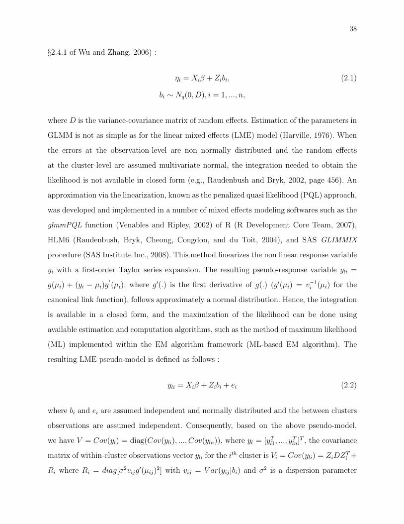
38
§2.4.1 of Wu and Zhang, 2006) :
ηi = Xiβ + Zibi, (2.1)
bi ∼ Nq(0, D), i = 1, ..., n,
where D is the variance-covariance matrix of random effects. Estimation of the parameters in
GLMM is not as simple as for the linear mixed effects (LME) model (Harville, 1976). When
the errors at the observation-level are non normally distributed and the random effects
at the cluster-level are assumed multivariate normal, the integration needed to obtain the
likelihood is not available in closed form (e.g., Raudenbush and Bryk, 2002, page 456). An
approximation via the linearization, known as the penalized quasi likelihood (PQL) approach,
was developed and implemented in a number of mixed effects modeling softwares such as the
glmmPQL function (Venables and Ripley, 2002) of R (R Development Core Team, 2007),
HLM6 (Raudenbush, Bryk, Cheong, Congdon, and du Toit, 2004), and SAS GLIMMIX
procedure (SAS Institute Inc., 2008). This method linearizes the non linear response variable
yi with a first-order Taylor series expansion. The resulting pseudo-response variable yli =
g(µi) + (yi − µi)g′(µi), where g′(.) is the first derivative of g(.) (g′(µi) = v−1
i (µi) for the
canonical link function), follows approximately a normal distribution. Hence, the integration
is available in a closed form, and the maximization of the likelihood can be done using
available estimation and computation algorithms, such as the method of maximum likelihood
(ML) implemented within the EM algorithm framework (ML-based EM algorithm). The
resulting LME pseudo-model is defined as follows :
yli = Xiβ + Zibi + ei (2.2)
where bi and ei are assumed independent and normally distributed and the between clusters
observations are assumed independent. Consequently, based on the above pseudo-model,
we have V = Cov(yl) = diag(Cov(yli), ..., Cov(yln)), where yl = [yTl1, ..., yTln]T , the covariance
matrix of within-cluster observations vector yli for the ith cluster is Vi = Cov(yli) = ZiDZTi +
Ri where Ri = diag[σ2vijg′(µij)
2] with vij = V ar(yij|bi) and σ2 is a dispersion parameter

39
which can be estimated from the usual residual sum of squares or fixed to 1 if the assumed
distribution does not have a scale parameter and no under- or over-dispersion parameter is
to be estimated.
Using the weights Wi = diag(wij) with wij = (vijg′(µij)
2)−1 and wij = vij for the
canonical link function, we derive the following weighted LME pseudo-model
W12i yli = W
12i Xiβ +W
12i Zibi +W
12i ei (2.3)
with Cov(W12i yli) = W
12i ZiD(W
12i Z)Ti +σ2Ini . This weighted LME pseudo-model can be fitted
using the ML-based EM algorithm.
The PQL algorithm is detailed below.
MACRO STEP 0. Set M = 0. Given initial estimates of the mean values, µ(0)ij , j =
1, ..., ni, fit a weighted LME pseudo-model using the linearized pseudo responses, y(0)li ,
and the weights, W(0)i = diag(w
(0)ij ).
Micro Step 0. Set m = 0. Let σ2(0) = 1, and D(0) = Iq.
Micro Step 1. Set m = m+ 1. Update β(m) and bi(m)
β(m) =
(n∑i=1
(W12
(M)
i Xi)T V −1
i(m−1)W12
(M)
i Xi
)−1( n∑i=1
(W12
(M)
i Xi)T V −1
i(m−1)W12
(M)
i y(M)li
),
bi(m) = D(m−1)(W12
(M)
i Zi)T V −1
i(m−1)
(W
12
(M)
i y(M)li −W
12
(M)
i Xiβ(m)
),
where Vi(m−1) = W12
(M)
i ZiD(m−1)(W12
(M)
i Zi)T + σ2
(m−1)Ini , i = 1, ..., n.
Micro Step 2. Update σ2(m), and D(m) using
σ2(m) = N−1
n∑i=1
{εTi(m)εi(m) + σ2
(m−1)[ni − σ2(m−1)trace(Vi(m−1))]
},
D(m) = n−1
n∑i=1
{bi(m)b
Ti(m) + [D(m−1) − D(m−1)(W
12
(M)
i Zi)T V −1
i(m−1)W12
(M)
i ZiD(m−1)]},
where εi(m) = W12
(M)
i y(M)li −W
12
(M)
i Xiβ(m) −W12
(M)
i Zibi(m).

40
Micro Step 3. Repeat steps 1 and 2 until convergence in terms of the generalized
log-likelihood value :
GLL(β, bi|y) =n∑i=1
{εTi(m)(σ2(m)Ini)
−1εi(m) + bTi(m)D−1(m)bi(m) + log |D(m)|+ log |σ2
(m)Ini|}.
MACRO STEP 1. Set M = M + 1. Set η(M−1)i = y
(M−1)li = Xiβ + Zibi, where β and bi
are the estimated values at the micro level convergence of the previous macro iteration.
Set µ(M)i = g−1(η
(M−1)i ), and fit a new weighted LME pseudo-model using the updated
y(M)li and W
(M)i , i.e. repeat the micro steps 0 to 3 using as initial values for σ2, and D,
their micro-level convergence values in the previous macro iteration.
MACRO STEP 2. Repeat macro step 1 until convergence of ηi.
The PQL algorithm is a doubly iterative process (i.e., micro iterations within macro
iterations). At each macro iteration, the linearized response variable and the weights are
updated. The micro iterations represent the iterative fitting process of a standard LME
model where the current linearized response variable and weights values serve as the response
variable and the weights, respectively.
2.3.2 PQL Algorithm for the Generalized Mixed Effects Regression Trees
The proposed generalized mixed effects regression tree (GMERT) model can be written
as :
ηi = f(Xi) + Zibi, (2.4)
bi ∼ Nq(0, D), i = 1, ..., n,
where all quantities are defined as in Section 2.3.1 except that the linear fixed part Xiβ in
(2.1) is replaced by the function f(Xi) that will be estimated with a standard regression tree
model. The random part, Zibi, is still assumed linear.
Following the PQL approach used to estimate the GLMM, we can derive a MERT

41
pseudo-model from the above GMERT model, exactly as the LME pseudo-model derived
from the GLMM. More precisely, a first-order Taylor-series expansion yields the linearized
response variable, yli = g(µi) + (yi − µi)g′(µi), and the MERT pseudo-model is defined as
follows :
yli = f(Xi) + Zibi + ei. (2.5)
The GMERT algorithm is basically the PQL algorithm used to fit GLMMs where the
weighted LME pseudo-model is replaced by a weighted MERT pseudo-model. Consequently,
the fixed-part f(Xi) is estimated with a standard regression tree model while the random
part, Zibi, is still estimated using a linear structure. The GMERT algorithm is detailed
below.
MACRO STEP 0. Set M = 0. Given initial estimates of the mean values, µ(0)ij , j =
1, ..., ni, fit a weighted MERT pseudo-model using the linearized pseudo responses,
y(0)li , and the weights, W
(0)i = diag(w
(0)ij ).
Micro Step 0. Set m = 0. Let bi(0) = 0, σ2(0) = 1, and D(0) = Iq.
Micro Step 1. Set m = m+ 1. Update y∗li(m), f(m)(Xi) and bi(m)
i) y∗li(m) = y(M)li − Zibi(m−1),
ii) Let f(m)(Xi) an estimate of f(Xi) obtained from a standard regression tree
algorithm with y∗li(m) as responses, Xi as covariates, and Wi as weights, i =
1, . . . , n . Note that the tree is built as usual using all N observations as
inputs along with their covariate vectors but with the specified weights (see
the appendix in Section 2.7 for details),
iii) bi(m) = D(m−1)(W12
(M)
i Zi)T V −1
i(m−1)
(W
12
(M)
i yMli −W12
(M)
i f(m)(Xi))
,
where Vi(m−1) = W12
(M)
i ZiD(m−1)(W12
(M)
i Zi)T + σ2
(m−1)Ini , i = 1, ..., n.

42
Micro Step 2. Update σ2(m), and D(m) using
σ2(m) = N−1
n∑i=1
{εTi(m)εi(m) + σ2
(m−1)[ni − σ2(m−1)trace(Vi(m−1))]
},
D(m) = n−1
n∑i=1
{bi(m)b
Ti(m) + [D(m−1) − D(m−1)(W
12
(M)
i Zi)T V −1
i(m−1)W12
(M)
i ZiD(m−1)]},
where εi(m) = W12
(M)
i y(M)li −W
12
(M)
i f(m)(Xi)−W12
(M)
i Zibi(m).
Micro Step 3. Repeat steps 1 and 2 until convergence in terms of the generalized
log-likelihood value :
GLL(f, bi|y) =n∑i=1
{εTi(m)(σ2(m)Ini)
−1εi(m) + bTi(m)D−1(m)bi(m) + log |D(m)|+ log |σ2
(m)Ini|}.
MACRO STEP 1. Set M = M + 1. Set η(M−1)i = y
(M−1)li = f(Xi) + Zibi, where f and
bi equal their estimated values at the micro level convergence of the previous macro
iteration. Set µ(M)i = g−1(η
(M−1)i ) and fit a new weighted MERT pseudo-model using
the updated y(M)li and W
(M)i , i.e., repeat the micro steps 0 to 3 using as initial values
for bi, σ2, and D, their micro-level convergence values in the previous macro iteration.
MACRO STEP 2. Repeat macro step 1 until convergence of ηi.
The GMERT model can be used to get the predicted response for a new observation
that belongs to a cluster among those used to fit this model as well as for a new observation
that belongs to a cluster not included in the sample used to fit this model. To predict the
response for a new observation that belongs to a cluster among those used to fit the gene-
ralized mixed effects regression tree model, we use both its corresponding fixed component
prediction and the predicted random part corresponding to its cluster. This is a cluster-
specific estimate. For a new observation that belongs to a cluster not included in the sample
used to estimate the model parameters, we can only use its corresponding fixed component
prediction (i.e., the random part is set to 0).

43
2.3.3 GMERT Model in the Binary Response Case
For clustered data with a binary response variable, i.e., yij = µij + εij with E(εij) = 0
and V ar(εij) = σ2vij = σ2µij(1 − µij), the commonly used parametric model is the mixed
effects logistic regression model with the logit link function, namely
ηij = g(µij) = logit(µij) = ln[µij
1− µij] = xTijβ + zTijbi. (2.6)
The conditional expectation µij = E(yij|bi, xij) = P (yij = 1|bi, xij) is the conditional pro-
bability of success given the random effects and covariate values. This model can also be
written as follows :
P (yij = 1|bi, xij) = g−1(ηij), (2.7)
where g−1(ηij) = 11+exp(−ηij) is the logistic cumulative distribution function.
The GMERT model in the binary response case (i.e., mixed effects classification tree)
and its corresponding MERT pseudo-model are respectively defined as follows :
ηij = ln[µij
1− µij] = f(xij) + zTijbi, (2.8)
ylij = ηij + eij, (2.9)
where eij = (yij − µij)g′(µij), g′(µij) = [µij(1 − µij)]−1, and V ar(eij) = σ2[µij(1 − µij)]−1.
The weights to be used in the GMERT algorithm are wij = µij(1− µij).
The GMERT model can be used to get a predicted probability of success for a new
observation that belongs to a cluster among those used to fit this model or for a new ob-
servation that belongs to a cluster not included in the sample used to fit this model. If the
new observation j belongs to a cluster i in the first category, then its predicted probability
of success µij equals 1
1+exp(−f(xij)−zTij bi), where f(xij) is its predicted fixed component that

44
results from the fixed tree rules and zTij bi is its predicted random part corresponding to its
cluster. However, if the new observation j belongs to a cluster i in the second category, then
its predicted probability µij equals 1
1+exp(−f(xij))(i.e., the random part is set to 0).
2.4 Simulation
In this section, we investigate the performance of the GMERT method for binary
outcomes in comparison to standard classification trees. The proposed GMERT method was
implemented in R by means of a repeated call to the MERT algorithm. The latter uses the
function rpart (Therneau and Atkinson, 1997). This function implements cost-complexity
pruning based on cross-validation after an initial large tree is grown. In order to ensure that
initial trees are sufficiently large, we set the complexity parameter to zero (i.e., cp = 0 means
that any split that does not decrease at all the overall lack of fit is also attempted). Though
there is a clear waste of computing time when not pruning off splits that are clearly not
worthwhile, doing so ensure that the two methods to be compared were given equal chance
to fit the data. In addition, we fixed the value of other parameters to reasonable (i.e., given
the true tree model and the generated data sample to be used) and equal levels. That is,
we set to five the maximum depth of any node of the final tree (i.e., maxdepth = 5), to
50 the minimum number of observations that must exist in a node in order for a split to
be attempted (i.e., minsplit = 50 ), and to 10 the minimum number of observations in any
terminal node (i.e., minbucket = 10). The largest tree is grown then pruned automatically
based on minimum ten-folds cross-validated error.
For GMERT models, we used the following schema to stop the macro-micro iteration
process and select a final model. Within each macro iteration, we follow the MERT algorithm
convergence process. More precisely, we first impose a minimum of 50 micro iterations to
avoid early stopping, then we keep iterating until either the absolute change in the generalized
log-likelihood, GLL, is less than 1E-06 or we reach a maximum of 200 micro iterations. Once
the stopping criterion is reached, we let the process continue for an additional 50 micro
iterations. We then find the most frequent (modal value) number of leaves for the selected

45
subtrees in the sequence of additional iterations. The final subtree model chosen at the micro
iteration level, is the one corresponding to the last micro iteration where the number of leaves
is equal to the modal value.
At the macro iteration level, we keep iterating until either the absolute change in ηi is
less than 1E-10 or we reach the maximum of 15 macro iterations. Once the stopping criterion
is reached, we let the process continue for an additional 5 macro iterations. We then find
the most frequent (modal value) number of leaves for the selected micro iteration subtrees
in the sequence of additional macro iterations. The final GMERT model chosen is the one
corresponding to the last macro iteration where the number of leaves is equal to the modal
value.
To compare the performance of standard and mixed effects classification trees, we eva-
luate their predictive accuracy measured by the predictive mean absolute deviation in terms
of the estimated probability (PMAD) and the predictive misclassification rate (PMCR).
2.4.1 Simulation Design
The simulation design used has a hierarchical structure of 100 clusters with 60 obser-
vations each. The first ten observations in each cluster form the training sample, and the
other 50 observations are left for the test sample. Consequently, the trees are built from
1000 observations (100 clusters of 10 observations). Eight random variables, X1 to X8, inde-
pendent and uniformly distributed in the interval [0, 10] are generated. Only the first five are
used predictors. The conditional or cluster-specific probabilities of success, µij, are generated
based on the following fixed tree rules along with the random component :
Leaf 1. If x1ij ≤ 5 and x2ij ≤ 5 then µij = g−1(g(ϕ1) + zTijbi),
Leaf 2. If x1ij ≤ 5 and x2ij > 5 and x4ij ≤ 5 then µij = g−1(g(ϕ2) + zTijbi),
Leaf 3. If x1ij ≤ 5 and x2ij > 5 and x4ij > 5 then µij = g−1(g(ϕ3) + zTijbi),
Leaf 4. If x1ij > 5 and x3ij ≤ 5 and x5ij ≤ 5 then µij = g−1(g(ϕ4) + zTijbi),
Leaf 5. If x1ij > 5 and x3ij ≤ 5 and x5ij > 5 then µij = g−1(g(ϕ5) + zTijbi),

46
Leaf 6. If x1ij > 5 and x3ij > 5 then µij = g−1(g(ϕ6) + zTijbi),
where g() is the logit link function, ϕ1 to ϕ6 are the typical probabilities of success (i.e.,
probability of success when the random effects bi equal zero), and bi ∼ N(0, D), for i =
1, ..., 100, j = 1, ..., 60 (see figure 2.1). Each observation j in cluster i falls into only one of
the six terminal nodes with a typical probability equal to ϕ1, ..., ϕ6 respectively. The binary
response values yij are generated according to a Bernoulli distribution using the rbinom
function of R with the size parameter fixed to one (i.e. one trial) and the prob parameter
fixed to µij (i.e. the generated conditional probability of success).
—————————-
Insert Figure 2.1 about here
—————————-
We consider 10 different data generating processes (DGP), summarized in Table 2.I.
Two different scenarios are selected for the fixed components. In the large fixed effects
scenario, the probabilities are chosen so that when there is no random effect, the standard
classification tree is able to recover the true number of leaves most of the time (i.e., about
95% of times). In the small fixed effects scenario, the probabilities are chosen so that when
there is no random effect, the standard classification tree is much less able to recover the
true number of leaves (i.e., about 55% of times only).
—————————-
Insert Table 2.I about here
—————————-
The random components are generated based on the following three different scenarios :
1. No random effects (NRE), i.e. D = 0.

47
2. Random intercept (RI), i.e. zij = 1 for i = 1, ..., 100, and j = 1, ..., 60, and D = d11 > 0.
3. Random intercept and covariate (RIC) which is a RI with a linear random effect for
X1. More precisely, zij = [1, x1ij] for i = 1, ..., 100, j = 1, ..., 60, and D =
d11 d12
d21 d22
,
d11 > 0, d22 > 0, and d12 = d21 = 0.
Within each fixed effects scenario with random effects, we consider two levels (low and
high) for the between-clusters covariance matrix D. More precisely, we consider that the
random effect is small (large) when it results in about 10% (30%) of the observations’ classes
being shifted from 1 to 0 or vice versa.
We adjust three models for each DGP scenario : 1) a standard (STD) classification
tree model, 2) a random intercept (RI) classification tree model, and 3) a random intercept
and covariate (RIC) classification tree model. The true model corresponds to the DGP used
to generate the data. In addition, using the glmmPQL function of R, we fitted for each DGP
scenario a parametric mixed effects logistic regression model (MElog) that uses the true
model leaves’ indicators as predictors and the true random effects structure. Clearly, this
model is not a real competitor since it is not possible in practice to specify this parametric
structure without knowing the true underlying data generating process. The MElog model
only serves as a benchmark for comparing the performance of the GMERT model. Overall,
we built 40 models (10 scenarios × 4 models). The simulation results are obtained by means
of 100 runs.
2.4.2 Simulation Results
Firstly, the performance of the methods is judged based on their predictive accuracy
on the test set as measured by : 1) the predictive mean absolute deviation (PMAD) in terms
of the estimated probability, and 2) the predictive misclassification rate (PMCR), i.e.,
PMAD =
∑100i=1
∑50j=1 |µij − µij|5000
,

48
PMCR =
∑100i=1
∑50j=1 |yij − yij|5000
,
where µij and yij are, respectively, the predicted probability and the predicted class of
observation j in cluster i in the test data set. Secondly, we compare the performance of the
GMERT approach to the MElog benchmark results.
The misclassification rate depends to some extent on the classification strategy and the
cutpoint value used to classify the observations, in particular, when the data has a nested
structure with clusters having different sizes in the training and the test data sets. The
adopted strategy consists in these steps :
1. Sort the distinct predicted probabilities of the observations in the training set (there
are, at most, number of clusters × number of terminal nodes distinct probabilities),
2. Classify the observations in the training set using in turn each one of these distinct
predicted probabilities as a cutpoint ; classify as class 1 each observation in the training
set that has a predicted probability equal to or higher than the cutpoint value,
3. Compute the proportions of class 1 that result from each one of the above cutpoint
values,
4. Find the predicted probability among those in step 1 that yields the closest proportion
of class 1 to the actual proportion of class 1 in the training set, and
5. Use this predicted probability as the cutpoint value in order to classify the observations
in the test set, i.e., classify as class 1 each observation in the test set that has a predicted
probability equal to or higher than this cutpoint value.
The average, median, minimum, maximum and standard deviation of the PMAD (co-
lumns 5 to 9) and the PMCR (columns 10 to 14) over the 100 runs were calculated and are
presented in Table 2.II.
—————————-
Insert Table 2.II about here

49
—————————-
In terms of predictive accuracy (PMAD and PMCR), we note that when random
effects are present (DGPs 3 to 10), the mixed effects classification tree does better than the
standard classification tree even with a wrong specification of the random component part.
The highest difference in terms of PMAD and PMCR is observed when both the fixed and
the random effects are somewhat large (i.e., 21.65% and 17.2% in DGP 4, and 20.23% and
17.06% in DGP 8, respectively). The lowest difference in terms of PMAD and PMCR is
observed when both the fixed and the random effects are somewhat small (i.e., 1.85% and
0.33% in DGP 5, and 1.82% and 0.46% in DGP 9, respectively). In addition, when there is
no random effect (DGPs 1 and 2), the standard classification tree algorithm does slightly
better in terms of PMAD and PMCR than the proposed GMERT approach with the highest
difference being less than 2% (i.e., 1.08% and 1.15% in DGP 1, and 1.38% and 1.90% in
DGP 2, respectively).
The difference in predictive accuracy (PMAD and PMCR) between the benchmark
model MElog and the GMERT model reaches a minimum when the fixed effects are large
while the random effects are small (DGPs 3 and 7), and a maximum when both the fixed and
the random effects are small (DGPs 5 and 9). In terms of PMAD, this difference equals 0.80%
and 1.13% in DGPs 3 and 7 respectively, and 2.50% and 2.25% in DGPs 5 and 9 respectively.
In terms of PMCR, this difference equals 0.69% and 1.02% in DGPs 3 and 7 respectively,
and 2.50% and 2.34% in DGPs 5 and 9 respectively. When there is no random effects, the
difference in predictive accuracy between the benchmark model MElog and the GMERT
model is, as anticipated, higher when the fixed effects are small (the PMAD difference in
DGP 2 is 2.63 times the PMAD difference in DGP 1, and the PMCR difference in DGP 2 is
2.56 times the PMCR difference in DGP 1).

50
2.5 Discussion
Earlier extensions of standard tree methods to the case of correlated data (Segal,
1992 ; Zhang, 1998 ; Abdolell, Leblanc, Stephens, and Harrison, 2002 ; Lee, 2005) do not
allow observation-level covariates to be candidates in the splitting process and, consequently,
1) no random or cluster-specific effect is allowed, and 2) all repeated observations from a
given subject remain together during the tree building process and can not be splitted across
different nodes. The MERT method (Hajjem et al., 2008) and the GMERT method proposed
in this paper can appropriately deal with the possible random effects of observation-level
covariates since these covariates are candidates in the splitting process. As a consequence,
the observations within clusters may be splitted.
The GMERT model is a cluster-specific or conditional model which yields cluster-
specific or conditional means estimates, µi = g−1(f(Xi)+Zibi), and not population-averaged
or marginal means estimates, E(µi).
Although the simulation study focused on the binary response case, the GMERT me-
thod can be tailored to other types of response variables (e.g., counts data, ordered catego-
rical outcomes, and multicategory nominal outcomes). Similarly to GLM, GMERT method
transforms the expected outcome using an appropriate link function according to the type
of the response variable and then equates it to a tree function of the fixed effects along with
a linear function of the random effects. Future research would be to look for a tree struc-
ture representation for the random component as well, which may be more suitable in more
complex problems.
2.6 Conclusion
In the present paper, we extended the mixed effect regression tree approach to other
types of outcomes (e.g., binary outcomes, counts data, ordered categorical outcomes, and
multicategory nominal scale outcomes).

51
The simulation results in the binary case show substantial improvements of the pre-
dictive accuracy over the standard classification tree, whenever random effects are present.
However, the main limit of tree based method, including the one proposed here, is their in-
stability. Ensemble methods such as bagging (Breiman, 1996) and forest of trees (Breiman,
2001) can greatly improve the predictive performance of trees. Hence, further improvement
of the predictive accuracy of the GMERT method could be achieved if we use it as the base
learner in an ensemble algorithms. This remains for future work.
An R program implementing the generalized mixed effects regression tree procedure is
available from the first author.

52
2.7 Appendix : Weighted Standard Regression Tree Within GMERT Algorithm
Here we clarify how the weights intervene in the standard regression tree fitted at each
micro iteration within the GMERT algorithm. At any micro iteration within a given macro
iteration, the standard regression tree uses the corresponding y∗li = yi−Zibi as the dependent
variable and Xi as the covariates, along with the weights Wi = diag(wij), with i = 1, ..., n
and j = 1, ..., ni.
Let T be the fitted standard regression tree, and let t be one of its nodes. Node t
contains a subset of Nt < N observations that belong to a subset of nt ≤ n clusters with
pseudo-responses y∗litjt , it = 1, ..., nt and jt = 1, ..., nit . Then, given the weights witjt of
observation jt in cluster it in node t, we have :
– The summary statistic to be attached to node t corresponds to its weighted response
average y∗lt =∑ntit=1
∑nitjt=1 witjty
∗litjt∑nt
it=1
∑nitjt=1 witjt
. This corresponds to the fitted value y∗lt = f(Xit)
when t is a terminal node.
– The error of node t equals its weighted sums of squares or corrected deviance DEVt,
with DEVt =∑nt
it=1
∑nitjt=1 witjt(y
∗litjt− y∗lt)2.
– The splitting criterion is the improvement or the percent change in the weighted
sums of squares for a given split of node t into two nodes tl and tr, i.e., Improve =
1− (DEVtl+DEVtr )
DEVt.
– The cross-validated relative error corresponding to a given complexity parameter
value for the tree T is defined as follows : xerror =∑ni=1
∑nij=1 wij(y
∗lij−y
∗l(−ij))
2
DEVroot, with
y∗l(−ij) being the predicted value for observation j in cluster i, from the standard
regression tree model that is fitted without this observation.

53
2.8 References
Abdollel, M., LeBlanc, M., Stephens, D. and Harrison, R. V. (2002). Binary partitioning forcontinuous longitudinal data : Categorizing a prognostic variable. Statistics in Medicine, 21,3395-3409.
Breiman, L., Friedman, J. H., Olshen, R. A., and Stone, C. J. (1984). Classification andregression trees. Wadsworth International Group. Belmont, California.
Breiman, L. (1996). Bagging predictors. Machine Learning, 24, 123-140.
Breiman, L. (2001). Random forests. Machine Learning, 45, 5-32.
Breslow, N.and Clayton, D. (1993). Approximate inference in generalized linear mixed mo-dels. Journal of the American Statistical Association, 88, 9-25.
Dempster, A. P., Laird, N. M., and Rubin, D. B. (1977). Maximum likelihood from incompletedata via the EM algorithm. Journal of the Royal Statistical Society, Series B, 39, 1-38.
Goldstein, H. and Rasbash, J. R. (1996). Improved Approximations for Multilevel Modelswith Binary Responses. Journal of the Royal Statistical Society, 159, 505-513.
Hajjem, A., Bellavance, F., and Larocque, D. (2008). Mixed Effects Regression Trees forClustered Data. Submitted. Les Cahiers du GERAD, G-2008-57.
Harville, D. A. (1976). Extension of the Gauss-Markov theorem to include the estimation ofrandom effects. Annals of Statistics, 4, 384-395.
Laird, N. M. and Ware, J. H. (1982). Random-effects models for longitudinal data. Biome-trics, 38, 963-974.
Lee, S. K. (2005). On Generalized multivariate decision tree by using GEE. ComputationalStatistics & Data Analysis, 49, 1105-1119.
McLachlan, G. J. and Krishman, T. (1997). The EM algorithm and extensions. New York :Wi-ley.
McCullagh, P. and Nelder, J. (1989). Generalized linear models (2nd Edition). Chapman &Hall/CRC. London.
R Development Team (2007). R : A Language and environment for statistical computing. RFoundation for Statistical Computing : www.R-project.org.
Raudenbush, S. W. and Bryk, A. S. (2002). Hierarchical linear models : Applications anddata analysis method (2nd Edition). Sage. Newbury Park, CA.
Raudenbush, S. W., Bryk, A. S., Cheong, Y. F., Congdon, R., and du Toit, M. (2004). HLM6 : Hierarchical Linear & Nonlinear Modeling. Scientific Software International, Inc.
SAS Institute Inc. (2008). SAS/STAT 9.2 User’s Guide : The GLIMMIX Procedure (Book

54
Excerpt). Cary, NC : SAS Institute Inc.
Segal, M. R. (1992). Tree-structured methods for longitudinal data. Journal of the AmericanStatistical Association, 87, 407-418.
Therneau, T. M. and Atkinson, E. J. (1997). An introduction to recursive partitioning usingthe rpart routines. Technical Report 61, Department of Health Science Research, Mayo Clinic,Rochester.
Venables, W. N. and Ripley, B. D. (2002). Modern Applied Statistics with S (Fourth edition).New York : Springer-Verlag.
Wu, H. and Zhang, J. T. (2006). Nonparametric regression methods for longitidunal dataanalysis : Mixed-effects modeling approaches. Wiley. New York.
Zhang, H. (1998). Classification trees for multiple binary responses. Journal of the AmericanStatistical Association, 93, 180-193.

55
Table 2.I Data generating processes (DGP) for the simulation study.
DGPData Structure
Fixed Component Random ComponentEffect ϕ1 ϕ2 ϕ3 ϕ4 ϕ5 ϕ6 Structure d11 d22
1 Large 0.10 0.20 0.80 0.20 0.80 0.90 No randomeffect
0.00 0.002 Small 0.20 0.40 0.70 0.30 0.60 0.80
3Large 0.10 0.20 0.80 0.20 0.80 0.90
Randomintercept
4.00 0.004 10.00 0.005
Small 0.20 0.40 0.70 0.30 0.60 0.800.50 0.00
6 4.00 0.00
7Large 0.10 0.20 0.80 0.20 0.80 0.90 Random
intercept andcovariate
2.00 0.058 5.00 0.259
Small 0.20 0.40 0.70 0.30 0.60 0.800.25 0.01
10 2.00 0.05
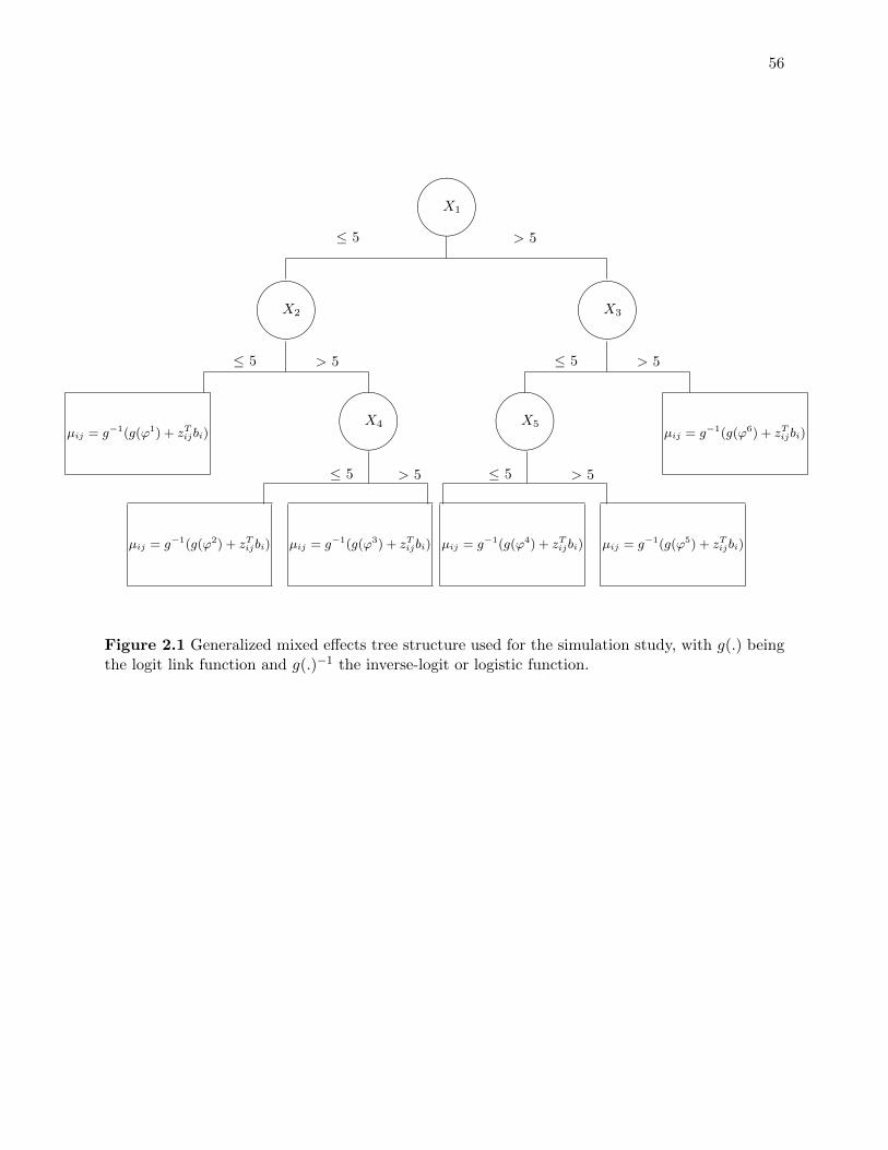
56
&%'$
X5
≤ 5 > 5
µij = g−1(g(ϕ4) + zTijbi) µij = g−1(g(ϕ5) + zTijbi)
&%'$
X4
≤ 5 > 5
µij = g−1(g(ϕ2) + zTijbi) µij = g−1(g(ϕ3) + zTijbi)
&%'$
X3
≤ 5 > 5
µij = g−1(g(ϕ6) + zTijbi)
&%'$
X2
≤ 5 > 5
µij = g−1(g(ϕ1) + zTijbi)
&%'$
X1
≤ 5 > 5
Figure 2.1 Generalized mixed effects tree structure used for the simulation study, with g(.) beingthe logit link function and g(.)−1 the inverse-logit or logistic function.

57
Table 2.II Results of the 100 simulation runs in terms of the predictive probability mean absolutedeviation (PMAD) and the predictive misclassification rate (PMCR).
DGPFixedeffect
Randomeffect
Fittedmodel∗
PMAD (%) PMCR (%)Avg. Med. Min Max Std Avg. Med. Min Max Std
1 LargeNorandomeffect
STD 3.09 3.05 1.48 6.38 0.97 15.71 15.67 13.92 18.20 0.79RI 3.86 3.66 1.28 8.85 1.46 16.86 16.58 14.54 21.44 1.52RIC 4.17 3.98 1.31 8.85 1.49 16.85 16.60 14.52 21.78 1.55MElog 2.48 2.36 0.78 4.80 0.87 15.49 15.39 13.86 17.62 0.71
2 Small
STD 4.97 4.64 1.73 11.98 1.89 29.33 28.94 26.94 34.68 1.63RI 6.35 5.95 2.23 13.36 2.81 31.23 30.41 26.74 38.82 2.83RIC 6.32 5.82 2.43 12.52 2.68 31.00 30.18 26.66 38.68 2.70MElog 2.73 2.72 0.86 5.34 0.82 27.72 27.76 26.22 29.12 0.68
3
Large
Randomintercept
STD 21.70 21.48 17.44 26.50 1.68 26.49 26.23 21.90 30.90 1.81RI 9.20 9.12 7.10 12.13 0.99 19.82 19.78 17.36 22.18 1.11RIC 9.69 9.58 7.10 14.87 1.20 20.08 20.02 17.82 22.86 1.16MElog 8.40 8.48 6.26 9.94 0.62 19.13 19.13 16.56 21.24 0.87
4
STD 30.24 29.97 25.29 35.50 1.98 33.65 33.23 28.92 41.14 2.58RI 8.59 8.52 6.80 11.42 0.84 16.45 16.46 12.20 20.16 1.16RIC 9.37 9.27 7.28 13.61 1.05 16.93 16.85 14.50 20.06 1.15MElog 7.59 7.57 6.06 9.14 0.65 15.69 15.73 11.82 18.34 1.07
5
Small
STD 12.56 12.36 10.40 15.97 1.30 31.70 31.36 29.06 36.44 1.67RI 10.71 10.54 7.81 15.44 1.58 31.37 31.17 28.14 36.58 1.62RIC 10.79 10.69 7.86 15.43 1.53 31.38 31.12 28.46 36.72 1.58MElog 8.21 8.17 6.61 9.89 0.60 28.87 28.85 27.46 30.64 0.64
6
STD 26.77 26.80 21.53 30.53 1.47 39.32 39.21 34.96 46.10 2.35RI 11.20 11.08 8.91 14.73 1.10 24.00 24.03 20.66 30.40 1.43RIC 11.40 11.20 9.32 14.66 1.02 24.09 24.06 20.94 30.30 1.42MElog 9.01 8.94 7.65 10.95 0.67 22.56 22.49 19.64 26.62 1.23
7
Large
Randominterceptandcovariate
STD 20.37 20.48 16.33 23.62 1.24 25.31 25.34 21.76 28.30 1.21RI 10.86 10.74 9.25 13.83 0.88 20.87 20.85 18.50 23.32 0.93RIC 10.58 10.47 8.43 14.14 0.98 20.83 20.79 18.02 23.54 1.02MElog 9.61 9.53 8.10 12.49 0.70 20.04 19.95 17.68 22.32 0.85
8
STD 30.90 30.92 27.43 35.56 1.60 34.34 33.97 30.06 42.52 2.37RI 12.37 12.35 9.91 15.76 0.98 18.15 18.20 15.10 20.82 1.14RIC 10.67 10.52 8.63 14.73 1.12 17.28 17.29 14.68 21.12 1.10MElog 9.45 9.39 7.91 11.35 0.74 16.42 16.37 14.16 18.60 0.92
9
Small
STD 12.86 12.64 10.21 17.48 1.45 31.81 31.15 29.00 37.92 1.85RI 11.12 10.73 8.87 16.57 1.62 31.36 30.93 28.12 36.82 1.86RIC 11.04 10.62 8.50 16.19 1.65 31.35 30.83 28.24 36.12 1.85MElog 8.79 8.73 7.77 10.44 0.50 29.01 28.99 26.98 30.78 0.71
10
STD 25.42 25.18 21.48 28.76 1.58 39.02 38.90 34.26 46.26 2.59RI 13.11 13.05 10.67 15.86 1.16 25.98 25.89 22.42 29.12 1.4RIC 12.54 12.48 10.23 15.16 1.09 25.84 25.72 22.74 29.82 1.38MElog 10.41 10.34 8.89 12.84 0.71 24.24 24.39 21.24 26.94 1.19
∗ STD : Standard tree ; RI : Random intercept tree ; RIC : Random intercept and covariate tree ; MElog : Mixed effect logistic

ARTICLE III
MIXED EFFECTS RANDOM FOREST FOR CLUSTERED DATA
Ahlem Hajjem, Francois Bellavance and Denis Larocque
...
Department of Management Sciences
HEC Montreal, 3000, chemin de la Cote-Sainte-Catherine,
Montreal, QC, Canada H3T 2A7

59
3.1 Abstract
This paper presents an extension of the well known random forest method to the case of clustered
data. The proposed “mixed effects random forest” method is implemented using a standard random forest
algorithm within the framework of the expectation-maximization (EM) algorithm. The simulation results
show that the proposed mixed effects random forest method provides substantial improvements over standard
random forest when the random effects are non negligible.
Keywords : Clustered data, mixed effects, regression tree, random forest.
3.2 Introduction
Tree based methods are well known and well appreciated by practitioners because they
often provide reasonable and easy to interpret models even when a large number of covariates
is present due to their ability to handle interactions automatically. However, the prediction
performance of a single tree can often be improved, at the expense of interpretability, by
using ensemble of trees. Bagging and the more general random forest algorithms (Breiman,
1996, 2001) are well known and very powerful ensemble methods for trees.
Using the mixed effects approach, Hajjem, Bellavance and Larocque (2008, 2010) ex-
tended the well known CART algorithm (Breiman, Friedman, Olshen and Stone, 1984) to
the case of clustered data. They proposed the mixed effects regression tree (MERT) algo-
rithm for a continuous outcome and the generalized mixed effects regression tree (GMERT)
algorithm for discrete outcomes in clustered data settings. Simulation results showed that
these methods provide substantial improvements over standard trees when the random ef-
fects are non-negligible. The key idea of MERT is to dissociate the fixed from the random
effects. It consists in the use of a standard regression tree algorithm within the framework
of the expectation-maximization (EM) algorithm. MERT is basically an iterative call to the
standard regression tree algorithm. At each iteration, the standard regression tree (SRT)
is applied to the original response from which the current estimate of the random effect
component is removed.

60
Following the same idea, one possibility for generalizing the standard random forest to
clustered data consists in replacing the SRT within each iteration of the MERT algorithm
with a standard forest of regression trees. The goal of the present paper is to introduce this
new random forest method, named “mixed effects random forest” (MERF), and to investigate
its performance with a simulation study. For that matter, the predictive performance of
MERF will be compared to that of five alternative models, including the standard random
forest, by varying some key features related to the strength of both the total and the random
effects and to the dependence between the predictors. The main finding is that MERF seems
to be more appropriate than a standard random forest for clustered data, particularly when
the random effects are non-negligible.
The remainder of this article is organized as follows : Section 3.3 describes the proposed
MERF approach ; Section 3.4 presents a simulation study to evaluate the performance of
MERF ; Section 3.5 gives some concluding remarks.
3.3 Mixed Effects Random Forest Approach
We define the mixed effects random forest (MERF) of regression trees as follows :
yi = f(Xi) + Zibi + εi,
bi ∼ Nq(0, D), εi ∼ Nni(0, Ri), (3.1)
i = 1, ..., n,
where yi = [yi1, ..., yini ]T is the ni× 1 vector of responses for the ni observations in cluster i,
Xi = [xi1, ..., xini ]T is the ni × p matrix of fixed-effects covariates, Zi = [zi1, ..., zini ]
T is the
ni × q matrix of random-effects covariates, εi = [εi1, ..., εini ]T is the ni × 1 vector of errors,
bi = (bi1, ..., biq)T is the q×1 unknown vector of random effects for cluster i, and the unknown
function f(Xi) is estimated using a standard forest of regression trees. The random part,
Zibi, is assumed linear. The total number of observations is N =∑n
i=1 ni. The covariance
matrix of bi is D while Ri is the covariance matrix of εi.

61
We further assume that bi and εi are independent and normally distributed and that
the between-clusters observations are independent. Hence, the covariance matrix of the vec-
tor of observations yi in cluster i is Vi = Cov(yi) = ZiDZTi + Ri, and V = Cov(y) =
diag(V1, . . . , Vn), where y = [yT1 , ..., yTn ]T . We will also assume that the correlation is induced
solely via the between-clusters variation, that is, Ri is diagonal (Ri = σ2Ini , i = 1, ..., n).
Basically, the MERF algorithm is the MERT algorithm (Hajjem et al., 2008) where
the single regression tree structure used to estimate the fixed part of the model is replaced
by an ensemble of unpruned regression trees (i.e. a forest). The out-of-bag estimates of the
standard forest are used to predict the response fixed part.
The MERF algorithm is as follows :
Step 0. Set r = 0. Let bi(0) = 0, σ2(0) = 1, and D(0) = Iq.
Step 1. Set r = r + 1. Update y∗i(r), f(Xi)(r), and bi(r)
i) y∗i(r) = yi − Zibi(r−1), i = 1, ..., n,
ii) Let f(Xi)(r) be an estimate of f(Xi) obtained from the out-of-bag predictions of
a standard random forest algorithm with y∗i(r) as the training set responses, Xi,
i = 1, . . . , n, as the corresponding training set of covariates, and taking as inputs
a selected number of bootstrap training samples drawn with replacement from the
training set (y∗i(r), Xi), i = 1, ..., n.
iii) bi(r) = D(r−1)ZTi V−1i(r−1)
(yi − f(Xi)(r)
), i = 1, ..., n,
where Vi(r−1) = ZiD(r−1)ZTi + σ2
(r−1)Ini , i = 1, ..., n.
Step 2. Update σ2(r), and D(r) using
σ2(r) = N−1
n∑i=1
{εTi(r)εi(r) + σ2
(r−1)[ni − σ2(r−1)trace(Vi(r−1))]
}D(r) = n−1
n∑i=1
{bi(r)b
Ti(r) + [D(r−1) − D(r−1)Z
Ti V−1i(r−1)ZiD(r−1)]
},
where εi(r) = yi − f(Xi)(r) − Zibi(r).

62
Step 3. Keep iterating by repeating steps 1 and 2 until convergence.
In words, the algorithm starts at step 0 with default values for bi, σ2, and D. At step
1, it first calculates the fixed part of the response variable, y∗i , i.e., the response variable
from which we remove the current available value of the random part. Second, the algorithm
takes bootstrap samples from the training set (y∗i , Xi) to build a forest of trees. To minimize
over fitting, the predicted fixed part f(xij) for observation j from cluster i is obtained with
the subset of trees in the forest that are build using the bootstrap samples not containing
observation j from cluster i (i.e. out-of-bag prediction). Third, it updates bi. At step 2, it
updates the variance components σ2 and D based on the residuals after the estimated fixed
component f(Xi) is removed from the raw data yi It keeps iterating by repeating steps 1
and 2 until convergence.
The convergence of the algorithm is monitored by computing, at each iteration, the
following generalized log-likelihood (GLL) criterion :
GLL(f, bi|y) =n∑i=1
{[yi − f(Xi)− Zibi]TR−1i [yi − f(Xi)− Zibi]
+ bTi D−1bi + log |D|+ log |Ri|}.
(3.2)
To predict the response for a new observation that belongs to a cluster among those
used to fit the MERF model, we use both its corresponding population-averaged random
forest prediction and the predicted random part corresponding to its cluster. For a new ob-
servation that belongs to a cluster not included in the sample used to estimate the model
parameters, we can only take the corresponding population-averaged random forest predic-
tion.
3.4 Simulation
We investigate the performance of the proposed mixed effects random forest of re-
gression trees through a simulation study. We compare the predictive mean squared error
(PMSE) of the MERF to that of five alternative models, namely, 1) the standard random

63
forest (SRF) of regression trees, 2) the mixed effects regression tree (MERT), 3) the standard
regression tree (SRT), 4) the linear mixed effect (LME) model, and 5) the linear model (LM).
We implemented the proposed MERF algorithm in R (R Development Core Team,
2007) using the package randomForest (Liaw and Wiener, 2002). The function randomFo-
rest implements Breiman’s random forest algorithm (based on Breiman and Cutler’s original
Fortran code) for classification and regression. Except for the parameter ntree which cor-
responds to the number of trees to grow within the forest, all the other default settings of
the function randomForest are used. To save overall computing time for the simulation, we
set the value of the parameter ntree to 300 instead of the default value of 500. Note that
this smaller number still ensures that every observation in the learning set gets predicted
by about 100 trees in each iteration since the out-of-bag set is formed by about 1/3 of the
original sample on average. The SRT and MERT models are also fitted with the default
settings of the function rpart (Therneau and Atkinson, 1997).
For MERF convergence, we suggest to force for a minimum number of iterations to
avoid early stopping then keep iterating until the absolute change in GLL is less than a
given small value (e.g. 1E-06). For the simulation, we however fixed the total number of
iterations to 300, regardless the behavior of GLL. Preliminary simulation runs showed that
GLL stabilizes between 50 and 250 iterations for the settings considered (see Subsection
§3.1). The final MERF model is the one at the last iteration. For MERT models, we force a
minimum of 50 iterations, then keep iterating while the absolute change in GLL is not less
than 1E-06 or we reach a maximum of 300 iterations. Once the stopping criterion is met,
we run an additional 50 iterations. The mixed tree model chosen is the one corresponding
to the last iteration where the number of leaves is equal to the modal value over the last 50
mixed tree models (Hajjem et al. 2008).
3.4.1 Simulation Design
The simulation design has a hierarchical structure of 100 unbalanced clusters and
5000 observations : 20 clusters with 10 observations, 20 with 30 observations, 20 with 50

64
observations, 20 with 70 observations, and 20 with 90 observations. The first 10% of the
generated observations in each cluster form the training sample, and the other 90% are kept
for the test sample. Consequently, the trees are built with 500 observations nested within
100 unbalanced clusters having 1, 3, 5, 7, or 9 observations. The remaining 4500 observations
form the test set.
The data generating process is as follows. Nine random variables are first generated
from a multivariate normal distribution (X1, ..., X9) ∼ N9(0,Σ) with Σ chosen such that
all variables have unit variance and are correlated with σk,k′ = ρ for k 6= k′ ≤ 9. Then,
the continuous response variable y is generated according to the following non linear model,
using only the first three random variables :
yij = m× g(xij) + bi + εij, (3.3)
g(xij) = 2x1ij + x22ij + 4(x3ij > 0) + 2 log |x1ij|x3ij,
bi ∼ N(0, σ2b ), εij ∼ N(0, σ2
ε),
i = 1, ..., 100, j = 1, ..., ni,
where m × g(xij) represents the response fixed part, with a non linear form and a variance
σ2Fixed = m2σ2
g . The parameter m simply serves as a tuning parameter to control the magni-
tude of σ2Fixed in the simulation design.
The proportion of total effects variability (PTEV) of the model in (3.3) is given by
PTEV =σ2Fixed + σ2
b
σ2Fixed + σ2
b + σ2ε
× 100, (3.4)
and the proportion of random effects variability (PREV) over total effects variability is
defined by
PREV =σ2b
σ2Fixed + σ2
b
× 100. (3.5)
We consider 12 different data generating processes (DGP), summarized in Table 3.I. In all

65
cases, the within cluster variance σ2ε is fixed at 1. We selected the values of 0 and 0.4 for ρ,
90% and 60% for PTEV (i.e. small and large noise), and 10%, 30%, and 50% for PREV (i.e.
small, moderate, and large random effects).
—————————-
Insert Table 3.I about here
—————————-
Note that σ2g depends only on the value of ρ. To estimate this variance, we conducted
for each value of ρ a simulation where g(xij) was generated one million times. The observed
variance was σ2g = 12.49 when ρ = 0, and σ2
g = 15.94 when ρ = 0.4. We used these values of
σ2g in equations (3.4) and (3.5) to obtain the values of m and σ2
b for each DGP in Table 3.I.
The simulation results are obtained by means of 100 runs.
3.4.2 Simulation Results
Table 3.II presents for each data generating process (DGP) the summary statistics
of the predictive mean squared error (PMSE) on the test set of the six fitted models. The
PMSE is computed as :
PMSE =
∑100i=1
∑nij=1(yij − yij)2
4500.
—————————-
Insert Table 3.II about here
—————————-
Table 3.III presents for each data generating process (DGP) the summary statistics of
the relative difference (RD) in PMSE between each alternative model and the MERF model :
RD =PMSEAlternative − PMSEMERF
PMSEAlternative× 100.

66
—————————-
Insert Table 3.III about here
—————————-
Figures 3.1 to 3.5 show for each DGP the distribution of the RD.
—————————-
Insert Figure 3.1 about here
—————————-
—————————-
Insert Figure 3.2 about here
—————————-
—————————-
Insert Figure 3.3 about here
—————————-
—————————-
Insert Figure 3.4 about here
—————————-
—————————-
Insert Figure 3.5 about here
—————————-

67
The primary interest of this simulation study is the comparison of MERF and SRF
(Figure 3.1). The main finding is that for a given value of PTEV and ρ, the benefit of MERF
over SRF increases as PREV increases. This can be seen by looking at the progression of
RD between DGP 1, 2 and 3 (PTEV = .9 and ρ = 0), between DGP 4, 5 and 6 (PTEV = .6
and ρ = 0), between DGP 7, 8 and 9 (PTEV = .9 and ρ = .4) and finally by looking at the
progression of RD between DGP 10, 11 and 12 (PTEV = .6 and ρ = .4). This result was
intuitively expected but this simulation study helps revealing how crucially the performance
of SRF depends on the PREV. The SRF is just not able to compensate for its omission of
taking the random effects into account and its performance worsen as the relative importance
of the random effects increases.
If we look into more details at the results, we can see that, except for few runs in
settings with relatively large noise and small random effects (i.e. PTEV = 60% and PREV
= 10% in DGPs 4 and 10), there is always some improvement (i.e. minimum RD > 0 ) of
MERF over each alternative model considered (Table 3.III, Figures 3.1 to 3.5). In all cases,
MERF did on average better (i.e. average RD > 0) than all the alternatives.
In all cases where the random effects are relatively small (i.e. PREV = 10% in DGPs 1,
4, 7, and 10), MERF average improvement over the alternative models vary between 16.02%
and 46.05%, except the ones over SRF which are much lower but still non negligible with
an average RD varying between 2.5%, and 10.65%. A failure to account for the correlation
among the observations may result in much less predictive performance, even in relatively
large noise and small random effects settings.
The most pronounced improvements of MERF over any alternative model appear in
settings with relatively small noise (i.e. PTEV = 90% in DGPs 1, 2, 3 and 7, 8, 9). In addition,
while the most pronounced improvements of MERF over models without random effect (i.e.
LM, SRT, and SRF) appear in settings with large random effects (i.e. PREV = 50% in
DGPs 3 and 9), the average RD between MERF and the other mixed effects models (i.e.
LME, and MERT) is higher in settings with small random effects (i.e. PREV = 10% in

68
DGPs 1 and 7). This is expected since the alternative mixed effects models take into account
the dependence of the data and estimate the random effects, as MERF do. Hence, when a
considerable proportion of the response variability is explained by the random effects, the
gap between their performance and that of MERF gets smaller.
In comparison to MERF improvement over LME, MERF improvement over MERT
seems to be relatively less affected by the PREV (see Figures 3.2 and 3.4). One additional
and interesting point to notice is the relatively huge variability of the improvement over
MERT in comparison to that over LME ; the standard deviations of the improvement over
MERT are more than twice those of the improvement over LME (Table 3.II, Figures 3.2 and
3.4).
The effect of the correlation between the predictors on the relative improvement of
MERF is basically absent in large noise settings, and small in small noise settings with
different trends depending on the alternative models. The average improvements over SRF,
MERT, and SRT seem to be slightly higher when the predictors are correlated than when
they are independent. In contrast, the average improvement over LME seems to be slightly
higher when the predictors are independent than when they are correlated. There is no clear
effect in the case of the alternative LM.
3.5 Concluding Remarks
One key feature of the random forest approach is the need to resample the observations.
With independent observations, using the standard bootstrap by resampling the individual
observations works perfectly. However, things are not straightforward with clustered data.
One key assumption of the approach proposed in this paper is that the random effects
totally explain the intra-cluster correlation. Hence, the observations are independent once
the random effects have been removed. This allows the use of standard bootstrap resampling
after removing the random effects from the responses (see Step 1 ii of the algorithm). The
simulation results showed that this approach seems reasonable, at least in the scenarios used.
A possibility for future work would be to investigate the robustness of the proposed approach

69
when the intra-cluster correlation is not entirely explained by the random effects.
Another entirely different approach would be to build directly a forest of MERTs. With
this approach, a bootstrap sample would be required for each individual MERT. However,
since the original observations are possibly correlated, taking a standard bootstrap sample
may not be the best choice. Bootstrapping directly clustered data can be done in different
ways (Field and Welsh, 2007). The three following strategies are possible : 1) resampling indi-
vidual observations (observation-bootstrap), 2) resampling entire clusters (cluster-bootstrap)
and 3) resampling of clusters and then of observations within them (two-stage-bootstrap).
One possibility for future work would be to investigate these strategies and compare them
to the approach proposed in this paper.
Finally, the proposed method is appropriate for a continuous outcome. Other types
of outcomes could be handled by using GMERT (Hajjem, Bellavance and Larocque, 2010)
instead of MERT. Specifically, one could replace the single weighted regression tree used to
estimate the pseudo-response fixed part in the doubly iterative GMERT algorithm with a
forest of weighted standard regression trees. Investigating this idea is left for future work.
The objective of this paper was to propose a way to build a forest of trees with clustered
data and to explore its performance. The results of the simulation study are promising and
the new approach could lead the way for future research on ensemble methods for clustered
data.
An R program implementing MERF is available from the first author.

70
3.6 References
Breiman, L., Friedman, J. H., Olshen, R. A., and Stone, C. J. (1984). Classification andregression trees. Wadsworth International Group. Belmont, California.
Breiman, L. (1996). Bagging predictors. Machine Learning, 24, 123-140.
Breiman, L. (2001). Random forests. Machine Learning, 45, 5-32.
Dempster, A. P., Laird, N. M., and Rubin, D. B. (1977). Maximum likelihood from incompletedata via the EM algorithm. Journal of the Royal Statistical Society, Series B, 39, 1-38.
Field, C. A. and Welsh, A. H. (2007). Bootstrapping clustered data. Journal of the RoyalStatistical Society, Series B, 69, 369-390.
Hajjem, A., Bellavance, F., and Larocque, D. (2008). Mixed Effects Regression Trees forClustered Data. Submitted. Les Cahiers du GERAD, G-2008-57.
Hajjem, A., Bellavance, F., and Larocque, D. (2010). Generalized Mixed Effects RegressionTrees. Les Cahiers du GERAD, G-2010-39.
Liaw, A. and Wiener, M. (2002). Classification and Regression by randomForest. R News,2, 18-22.
McLachlan G. J. and Krishman T. (1997). The EM algorithm and extensions. Wiley. NewYork.
R Development Team (2007). R : A Language and environment for statistical computing. RFoundation for Statistical Computing : www.R-project.org.
Therneau, T. M. and Atkinson, E. J. (1997). An introduction to recursive partitioning usingthe rpart routines. Technical Report 61, Department of Health Science Research, Mayo Clinic,Rochester.

71
Table 3.I Data generating processes (DGP) for the simulation study.
DGP ρ PTEV∗ PREV∗∗ σ2Fixed m σ2
b ICC∗∗∗
1
0.0
9010 8.1 0.8 0.9 47.4
2 30 6.3 0.7 2.7 73.03 50 4.5 0.6 4.5 81.84
6010 1.4 0.3 0.2 13.0
5 30 1.1 0.3 0.5 31.06 50 0.8 0.2 0.8 42.9
7
0.4
9010 8.1 0.7 0.9 47.4
8 30 6.3 0.6 2.7 73.09 50 4.5 0.5 4.5 81.810
6010 1.4 0.3 0.2 13.0
11 30 1.1 0.3 0.5 31.012 50 0.8 0.2 0.8 42.9
∗Proportion of Total Effects Variability =σ2Fixed+σ
2b
σ2Fixed
+σ2b+σ2
ε× 100
∗∗Proportion of Random Effects Variability =σ2b
σ2Fixed
+σ2b
× 100
∗∗∗Intra Cluster Correlation =σ2b
σ2b+σ2
ε× 100

72
Tab
le3.I
IR
esu
lts
ofth
ep
red
icti
vem
ean
squ
ared
erro
r(P
MS
E)
ofM
ER
F,
SR
F,
ME
RT
,S
RT
,L
ME
,an
dL
Mm
od
els
base
don
100
sim
ula
tion
run
s.
DG
PM
ER
FSR
FM
ER
TSR
TL
ME
LM
Avg.
Med
Min
Max
Std
Avg.
Med
Min
Max
Std
Avg.
Med
Min
Max
Std
Avg.
Med
Min
Max
Std
Avg.
Med
Min
Max
Std
Avg.
Med
Min
Max
Std
14.
06
4.03
3.40
4.80
0.28
4.55
4.5
53.
605.
530.
315.4
25.
374.
26
9.2
80.
71
6.0
05.9
54.
57
8.9
10.7
37.1
27.1
16.2
87.8
90.3
17.5
27.5
46.
398.4
10.
342
3.67
3.65
3.10
4.57
0.26
5.86
5.8
54.
727.
460.
514.8
44.
693.
63
8.1
30.
67
7.2
47.1
05.
52
9.7
10.7
86.0
86.0
85.6
26.6
40.2
37.9
87.9
56.
759.3
50.
493
3.01
2.97
2.53
3.69
0.20
7.28
7.2
64.
739.
270.
773.8
63.
833.
01
5.5
80.
51
8.5
58.6
26.
29
11.0
90.9
44.7
34.7
34.2
95.1
90.1
98.5
68.5
56.
0510
.53
0.69
41.
63
1.62
1.45
1.83
0.07
1.67
1.6
71.
511.
890.
071.9
51.
941.
63
2.3
20.
14
2.0
22.0
11.
69
2.4
10.1
42.0
72.0
61.8
92.2
90.0
72.1
02.1
11.
942.3
30.
075
1.60
1.60
1.44
1.75
0.06
1.91
1.9
01.
692.
170.
101.8
91.
891.
63
2.2
70.
14
2.2
52.2
51.
87
2.5
60.1
51.9
21.9
21.7
72.1
00.0
52.2
02.1
92.
012.4
50.
096
1.53
1.53
1.38
1.66
0.06
2.14
2.1
21.
862.
450.
131.7
61.
771.
57
2.0
80.
09
2.4
12.3
82.
04
2.8
10.1
61.7
41.7
41.6
01.9
00.0
52.3
12.3
02.
062.5
80.
12
73.
22
3.20
2.78
4.06
0.22
3.75
3.7
13.
294.
560.
274.4
54.
413.
65
5.7
80.
42
5.0
24.9
24.
20
6.1
80.4
85.2
25.1
94.7
65.7
20.2
15.7
05.6
75.
216.4
20.
268
2.93
2.93
2.55
3.43
0.17
5.31
5.2
74.
186.
620.
513.9
63.
933.
12
5.4
80.
45
6.6
06.5
35.
10
8.4
00.7
34.5
04.4
94.1
05.0
70.1
96.6
76.6
55.
478.0
50.
529
2.51
2.51
2.19
3.00
0.15
6.87
6.9
25.
0710
.03
0.8
13.3
63.
332.
73
5.1
30.
37
8.1
18.1
06.
08
11.4
70.9
43.6
53.6
53.3
34.0
20.1
47.6
87.7
55.
9810
.63
0.79
101.
47
1.47
1.35
1.59
0.05
1.53
1.5
21.
371.
670.
051.7
81.
781.
51
2.0
40.
10
1.8
51.8
41.
56
2.1
00.1
21.7
51.7
51.6
21.8
90.0
51.8
01.8
01.
641.9
20.
0511
1.48
1.48
1.36
1.61
0.05
1.79
1.7
81.
562.
100.
091.7
51.
741.
50
2.0
20.
10
2.0
82.0
71.
82
2.3
90.1
11.6
81.6
81.5
61.8
10.0
51.9
71.9
61.
772.2
60.
0912
1.43
1.43
1.34
1.56
0.04
2.02
2.0
11.
702.
440.
151.6
61.
641.
47
1.9
70.
09
2.2
52.2
41.
90
2.6
90.1
61.5
61.5
61.4
71.6
70.0
42.1
22.0
91.
812.5
10.
15
Tab
le3.I
IIR
elat
ive
diff
eren
ce(R
D∗ )
inP
MS
Eb
etw
een
ME
RF
and
each
one
ofth
eal
tern
ativ
em
od
els
:S
RF
,M
ER
T,
SR
T,
LM
E,
an
dL
M.
DG
PSR
FM
ER
TSR
TL
ME
LM
Avg.
Med
Min
Max
Std
Avg.
Med
Min
Max
Std
Avg.
Med
Min
Max
Std
Avg.
Med
Min
Max
Std
Avg.
Med
Min
Max
Std
110
.65
10.7
51.
4919.
553.3
524
.34
23.8
74.
20
51.4
17.
9231
.70
30.4
517.8
749.3
77.0
342.9
843.3
534.0
948.7
22.8
546.0
546.5
937
.91
51.4
72.
91
236
.95
36.7
520
.62
50.8
26.
0823
.29
22.9
85.
66
53.7
17.
9448
.82
48.9
125.6
660.0
75.8
553.8
553.8
442.0
261.0
73.2
253.8
553.8
442
.02
61.0
74.
09
358
.28
58.9
637
.81
69.0
44.
6421
.23
21.4
82.
65
39.6
28.
1064
.48
64.8
353.1
074.1
23.9
736.3
836.3
125.2
042.8
43.1
264.6
664.8
651
.35
72.7
33.
37
42.
502.
46-2
.60
6.84
1.65
16.0
215
.55
5.99
26.6
74.
5418
.93
18.6
39.2
628.
46
4.5
321.0
921.0
615.4
427.0
92.0
822.5
422.2
616
.80
29.2
52.
16
516
.13
15.9
37.
5425.
323.6
514
.99
15.8
40.
47
29.8
35.
4128
.49
28.3
412.8
338.1
14.4
316.7
516.9
29.7
122.
17
2.4
427.2
527.0
619
.62
34.3
33.
23
628
.35
28.6
819
.51
37.4
64.
1213
.03
13.5
92.
93
23.0
54.
1136
.36
36.0
626.3
045.0
44.0
712.4
412.4
45.1
117.
46
2.3
933.7
233.7
124
.57
42.1
83.
60
714
.12
13.7
05.
9224.
674.1
927
.27
27.2
412
.16
46.3
56.8
835
.45
35.3
121.1
551.2
56.3
638.3
638.3
927.9
545.9
72.9
943.5
443.4
934
.92
52.0
33.
20
844
.39
44.8
927
.50
56.7
55.
4225
.31
25.0
87.
66
44.0
87.
0255
.14
55.6
142.3
664.8
44.8
634.9
134.7
529.4
041.7
52.5
555.8
355.9
744
.63
65.4
83.
76
963
.01
63.4
252
.58
74.5
34.
3424
.52
24.3
76.
54
41.5
57.
2068
.68
69.0
958.6
076.8
33.6
731.1
131.0
823.4
337.3
53.0
966.9
967.4
256
.56
75.8
53.
54
103.
473.
40-0
.40
8.95
1.77
17.1
816
.84
3.76
27.3
74.
2519
.99
19.6
36.8
129.
49
4.5
815.7
315.7
410.3
920.6
72.3
218.0
018.1
211
.33
23.4
02.
38
1117
.05
17.0
88.
8727.
763.6
115
.22
15.4
06.
87
25.6
73.
7728
.50
28.2
018.0
436.3
43.5
611.9
711.8
87.3
916.
38
1.8
324.6
424.6
516
.93
32.8
63.
16
1228
.81
28.7
515
.85
42.3
45.
0613
.50
13.3
04.
92
25.5
03.
8336
.19
36.0
325.6
147.8
74.3
98.4
28.6
93.
54
14.0
92.1
132.0
732.4
620
.89
44.0
94.
68
∗R
elati
ve
Diff
eren
cein
PM
SE
=PMSE
Alt
ernative−PMSE
ME
RF
PMSE
Alt
ernative
×100

73
● ●
●●
●●
● ●●
●●
●●
●
● ● ●●
12
34
56
78
910
1112
0204060
Dat
a G
ener
atin
g P
roce
sses
Relative Difference in PMSE
Inde
pend
ent p
redi
ctor
s, i.
e. ρ
= 0
Dep
ende
nt p
redi
ctor
s, w
ith ρ
= .4
PT
EV
= .9
PT
EV
= .6
PT
EV
= .9
PT
EV
= .6
PR
EV
=
.1.3
.5
PR
EV
=
.1.3
.5
PR
EV
=
.1.3
.5
PR
EV
=
.1.3
.5
Fig
ure
3.1
Dis
trib
uti
onov
erth
e10
0si
mu
lati
onru
ns
ofth
ere
lati
ved
iffer
ence
inP
MS
Eb
etw
een
ME
RF
and
SR
F
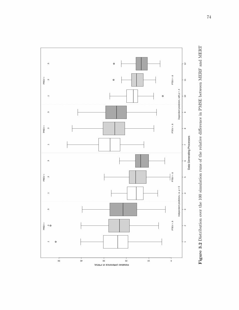
74
●
●
●
●●
12
34
56
78
910
1112
01020304050
Dat
a G
ener
atin
g P
roce
sses
Relative Difference in PMSE
Inde
pend
ent p
redi
ctor
s, i.
e. ρ
= 0
Dep
ende
nt p
redi
ctor
s, w
ith ρ
= .4
PT
EV
= .9
PT
EV
= .6
PT
EV
= .9
PT
EV
= .6
PR
EV
=
.1.3
.5
PR
EV
=
.1.3
.5
PR
EV
=
.1.3
.5
PR
EV
=
.1.3
.5
Fig
ure
3.2
Dis
trib
uti
onov
erth
e10
0si
mu
lati
onru
ns
ofth
ere
lati
ved
iffer
ence
inP
MS
Eb
etw
een
ME
RF
and
ME
RT
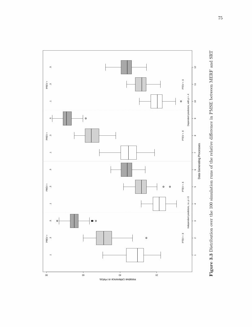
75
●
● ● ●● ●●
● ●
●
●
12
34
56
78
910
1112
20406080
Dat
a G
ener
atin
g P
roce
sses
Relative Difference in PMSE
Inde
pend
ent p
redi
ctor
s, i.
e. ρ
= 0
Dep
ende
nt p
redi
ctor
s, w
ith ρ
= .4
PT
EV
= .9
PT
EV
= .6
PT
EV
= .9
PT
EV
= .6
PR
EV
=
.1.3
.5
PR
EV
=
.1.3
.5
PR
EV
=
.1.3
.5
PR
EV
=
.1.3
.5
Fig
ure
3.3
Dis
trib
uti
on
over
the
100
sim
ula
tion
run
sof
the
rela
tive
diff
eren
cein
PM
SE
bet
wee
nM
ER
Fan
dS
RT
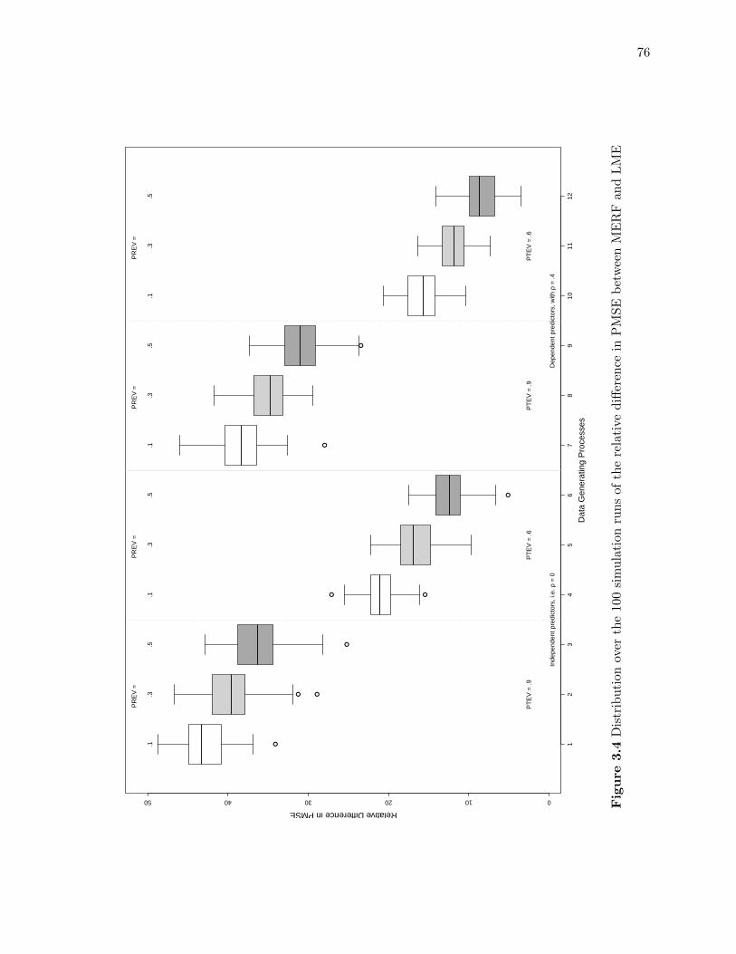
76
●
●●
●
● ●
●
●
●
12
34
56
78
910
1112
01020304050
Dat
a G
ener
atin
g P
roce
sses
Relative Difference in PMSE
Inde
pend
ent p
redi
ctor
s, i.
e. ρ
= 0
Dep
ende
nt p
redi
ctor
s, w
ith ρ
= .4
PT
EV
= .9
PT
EV
= .6
PT
EV
= .9
PT
EV
= .6
PR
EV
=
.1.3
.5
PR
EV
=
.1.3
.5
PR
EV
=
.1.3
.5
PR
EV
=
.1.3
.5
Fig
ure
3.4
Dis
trib
uti
on
over
the
100
sim
ula
tion
run
sof
the
rela
tive
diff
eren
cein
PM
SE
bet
wee
nM
ER
Fan
dL
ME
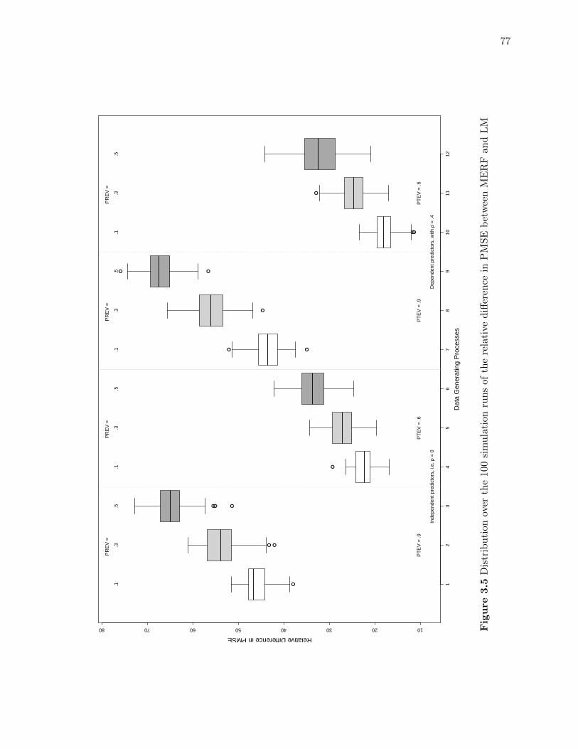
77
●
●●
●●●
●
●●
●
● ●
●●
●
12
34
56
78
910
1112
1020304050607080
Dat
a G
ener
atin
g P
roce
sses
Relative Difference in PMSE
Inde
pend
ent p
redi
ctor
s, i.
e. ρ
= 0
Dep
ende
nt p
redi
ctor
s, w
ith ρ
= .4
PT
EV
= .9
PT
EV
= .6
PT
EV
= .9
PT
EV
= .6
PR
EV
=
.1.3
.5
PR
EV
=
.1.3
.5
PR
EV
=
.1.3
.5
PR
EV
=
.1.3
.5
Fig
ure
3.5
Dis
trib
uti
onov
erth
e10
0si
mu
lati
onru
ns
ofth
ere
lati
ved
iffer
ence
inP
MS
Eb
etw
een
ME
RF
and
LM

CONCLUSION GENERALE
Dans cette these par articles, nous avons propose une approche simple pour rendre plus
appropriees les methodes d’arbres et de forets aleatoires standards lorqu’on veut les appliquer
aux donnees hierarchiques. Il s’agit des arbres et des forets aleatoires a effets mixtes.
Dans le premier article, nous avons propose la methode d’arbre nommee “mixed effects
regression tree” (MERT). Elle etend la methode d’arbre de regression standard aux donnees
hierarchiques avec une reponse continue. Sur la base d’une etude de simulation, nous avons
pu demontrer que ne pas tenir compte de la dependance des donnees nuit a la capacite de
l’algorithme standard d’identifier le vrai lien entre la reponse et les covariables. En tenant
compte de cette dependance, MERT reussit mieux ce defi. En modelisant la partie fixe de
la variable reponse par une structure d’arbre, MERT a assouplit l’hypothese de la linearite
de la partie fixe dans le modele de regression lineaire a effets mixtes. En procedant toujours
par une structure d’arbre, des travaux futurs pourraient tenter d’assouplir aussi l’hypothese
de la linearite de la partie aleatoire, et/ou celle de l’additivite de ces deux parties.
Dans le deuxieme article, nous avons propose une methode nomme “generalized mixed
effects regression tree” (GMERT). Elle etend la methode MERT a d’autres types de reponses
(reponses binaires, donnees de comptage, reponses categorielles ordonnees, reponses multi-
categorielles nominales). Tout comme le modele lineaire generalise (McCullagh and Nelder,
1989), le modele GMERT transforme la reponse esperee en utilisant une fonction de lien
appropriee selon le type de la variable reponse, et l’apparie a une fonction d’arbre des ef-
fets fixes en plus d’une fonction lineaire des effets aleatoires. Le modele GMERT est par
consequent un modele conditionnel qui genere des estimations conditionnelles et non pas des
estimations marginales.

79
Dans le troisieme article, nous avons propose une methode de foret aleatoire a effets
mixtes. Nous avons nommee cette methode “mixed effects random forest” (MERF). Nous
l’avons implemente en utilisant une foret d’arbres de regression standards a l’interieur de l’al-
gorithme EM. Plus precisement, a chaque iteration de l’algorithme EM, les predictions “out-
of-bag” d’une foret aleatoire standard sont utilisees pour estimer la partie fixe de la variable
reponse mesuree sur une echelle continue. Il serait certainement utile d’etendre MERF a
d’autres types de reponses. Une idee simple serait de remplacer l’arbre de regression standard
pondere, utilise pour estimer la partie fixe de la pseudo-reponse dans l’algorithme double-
ment iteratif GMERT, par une foret d’arbres de regression standards ponderes. Il serait aussi
interessant de comparer GMERT a une approche alternative qui consisterait dans la construc-
tion d’une foret aleatoire d’arbres MERT en utilisant des strategies de reechantillonage
appropriees pour des donnees hierarchiques, comme par exemple un reechantillonnage au
niveau groupe, ou un reechantillonnage en deux etapes, c.a.d, un reechantillonnage au ni-
veau groupe suivi d’un reechantillonnage au niveau observation a l’interieur des groupes deja
echantillonnes.
Les extensions anterieures des methodes d’arbres standards aux donnees correlees (Se-
gal, 1992 ; Zhang, 1998 ; Abdolell, Leblanc, Stephens, and Harrison, 2002 ; Lee, 2005) ne
permettent pas que les covariables du niveau observation entrent comme candidates dans
le processus d’embranchement, et par consequent, 1) aucun effet aleatoire ou specifique au
groupe n’est modelisable, et 2) toutes les observations provenant d’un meme sujet restent
ensemble tout au long de ce processus et ne peuvent pas etre separees dans des noeuds
differents. La methode d’arbre a effets mixtes que nous avons propose traite de facon ap-
propriee les effets aleatoires potentiels des covariables du niveau observation. En plus, ces
dernieres sont candidates dans le processus d’embranchement de l’arbre a effets mixtes. Par
consequent, les observations intra-groupe pourraient etre separees dans des noeuds differents.
Toutefois, l’arbre a effets mixtes suppose que la correlation decoule uniquement de la varia-
tion inter-groupes. Il serait donc utile de la generaliser afin de permettre la modelisation de
structures alternatives de covariances intra-groupe. Une idee a investiguer serait de rempla-

80
cer l’algorithme EM utilise jusqu’ici par l’algorithme EM hybride de Jennrich et Schluchter
(1986).
Notre implementation de l’arbre a effets mixtes fait en sorte que tous les avantages
de l’arbre standard comparativement aux modeles de regression parametriques s’etendent
naturellement aux arbres a effets mixtes. Par exemple, tout comme les arbres standards, les
arbres a effets mixtes sont des modeles qui peuvent etre representes graphiquement et qui
sont facilement interpretables. Il faut neanmoins rester prudent et investiguer la robustesse de
cette approche lorsque certaines de ses hypotheses ne sont pas verifiees, soient la non linearite
de la partie aleatoire, la non additivite de la partie fixe et aleatoire, la non normalite des
erreurs, et/ou la presence d’une correlation induite a la fois par la variation inter- et intra-
groupes.

BIBLIOGRAPHIE
Abdollel, M., LeBlanc, M., Stephens, D. and Harrison, R. V. (2002). Binary partitio-ning for continuous longitudinal data : Categorizing a prognostic variable. Statisticsin Medicine, 21, 3395-3409.
Breiman, L., Friedman, J. H., Olshen, R. A., and Stone, C. J. (1984). Classifi-cation and regression trees. Wadsworth International Group. Belmont, California.
Breiman, L. (1996). Bagging predictors. Machine Learning, 24, 123-140.
Breiman, L. (2001). Random forests. Machine Learning, 45, 5-32.
Breslow, N.and Clayton, D. (1993). Approximate inference in generalized linearmixed models. Journal of the American Statistical Association, 88, 9-25.
Bryk, A. S., and Raudenbush, S. W. (1987). Application of hierarchical linearmodels to assessing change. Psychological Bulletin, 101, 147-158.
Davidian, M. and Giltinan, D. M. (1995). Nonlinear Mixed Effects Models forRepeated Measurement Data. Chapman and Hall.
Dempster, A. P., Laird, N. M., and Rubin, D. B. (1977). Maximum likelihoodfrom incomplete data via the EM algorithm. Journal of the Royal Statistical Society,Series B, 39, 1-38.
Field, C. A. and Welsh, A. H. (2007). Bootstrapping clustered data. Journalof the Royal Statistical Society, Series B, 69, 369-390.
Fitzmaurice, G. M., Laird, N. M., and Ware, J. H. (2004). Applied longitidunalanalysis. New York : Wiley.
Ghattas, B., and Nerini, D. (2007). Classifying densities using functional regressiontrees : Applications in oceanology. Computational Statistics & Data Analysis, 51,4984-4993.
Goldstein, H. (2003). Multilevel statistical models (3rd Edition). Arnold, Lon-don.
Goldstein, H. and Rasbash, J. R. (1996). Improved Approximations for Multi-level Models with Binary Responses. Journal of the Royal Statistical Society, 159,505-513.
Harville, D. A. (1976). Extension of the Gauss-Markov theorem to include the

82
estimation of random effects. Annals of Statistics, 4, 384-395.
Harville, D. A. (1977). Maximum likelihood approaches to variance componentestimation and to related problems. Journal of the American Statistical Association,72, 320-38.
Jennrich, R. I., and Schluchter, M. D. (1986). Unbalanced Repeated-Measureswith Structured Covariance Matrices. Biometrics, 42, 805-820.
Kuhnert, P. M., Do, K.-A., and McClure, R. (2000). Combining nonparametricmodels with logistic regression : An application to motor vehicle injury data.Computational Statistics and Data Analysis, 34, 371-386.
Laird, N. M. and Ware J. H. (1982). Random-effects models for longitudinaldata. Biometrics, 38, 963-974.
Lee, S. K. (2005). On Generalized multivariate decision tree by using GEE.Computational Statistics & Data Analysis, 49, 1105-1119.
Liaw, A. and Wiener, M. (2002). Classification and Regression by randomFo-rest. R News, 2, 18-22.
McCullagh, P. and Nelder, J. (1989). Generalized linear models (2nd Edition).Chapman & Hall/CRC. London.
McLachlan G. J. and Krishman T. (1997). The EM algorithm and extensions.Wiley. New York.
R Development Team (2007). R : A Language and environment for statisticalcomputing. R Foundation for Statistical Computing : www.R-project.org.
Raudenbush, S. W. and Bryk, A. S. (2002). Hierarchical linear models : Appli-cations and data analysis method (2nd Edition). Sage. Newbury Park, CA.
Raudenbush, S. W., Bryk, A. S., Cheong, Y. F., Congdon, R., and du Toit,M. (2004). HLM 6 : Hierarchical Linear & Nonlinear Modeling. Scientific SoftwareInternational, Inc.
SAS Institute Inc. (2008). SAS/STAT 9.2 User’s Guide : The GLIMMIX Pro-cedure (Book Excerpt). Cary, NC : SAS Institute Inc.
Segal, M. R. (1992). Tree-structured methods for longitudinal data. Journal ofthe American Statistical Association, 87, 407-418.
Simonoff, J. S. and Sparrow, I. R. (2000). Predicting movie grosses : Winnersand losers, blockbusters and sleepers. Chance, 13(3), 15-24.
Therneau, T. M. and Atkinson, E. J. (1997). An introduction to recursive par-

83
titioning using the rpart routines. Technical Report 61, Department of Health ScienceResearch, Mayo Clinic, Rochester.
Venables, W. N. and Ripley, B. D. (2002). Modern Applied Statistics with S(Fourth edition). New York : Springer-Verlag.
Wu, H. and Zhang, J. T. (2006). Nonparametric regression methods for longiti-dunal data analysis : Mixed-effects modeling approaches. Wiley. New York.
Yu, Y. and Lambert, D. (1999). Fitting Trees to Functional Data : With anApplication to Time-of-day Patterns. Journal of Computational and GraphicalStatistics, 8, 749-762.
Zhang, H., (1997). Multivariate Adaptive Splines for Analysis of LongitudinalData. Journal of Computational and Graphical Statistics, 6, 74 - 91.
Zhang, H., (1998). Classification trees for multiple binary responses. Journal ofthe American Statistical Association, 93, 180-193.
Zhang, D. and Davidian, M. (2004). Likelihood and conditional likelihood in-ference for generalized additive mixed models for clustered data. Journal ofMultivariate Analysis, 91, 90-106.