measurement and modeling of thermodynamic and...

MEASUREMENT AND MODELING OF THERMODYNAMIC AND KINETIC DATA OF

MEMBRANE-FORMING SYSTEMS

A Thesis Submitted to The Graduate School of Engineering and Science of

�zmir Institute of Technology in Partial Fulfillment of the Requirements for the Degree of

MASTER OF SCIENCE

in Chemical Engineering

by Mine Özge ARSLAN

September 2007 �ZM�R

We approve the thesis of Mine Özge ARSLAN

Date of Signature

…………………………….................... 14 September 2007

Assoc. Prof. Dr. Sacide ALSOY ALTINKAYA

Supervisor

Department of Chemical Engineering

�zmir Institute of Technology

…………………………….................... 14 September 2007

Assoc. Prof. Dr. Funda TIHMINLIO�LU

Department of Chemical Engineering


…………………………….................... 14 September 2007

Assoc. Prof. Dr. Metin TANO�LU

Department of Mechanical Engineering


…………………………….................... 14 September 2007

Prof. Dr. Devrim BALKÖSE

Head of Department �zmir Institute of Technology

…….……………………………

Prof. Dr. M. Barı� ÖZERDEM

Head of Graduate School

ACKNOWLEDGEMENTS

I would like to thank to my advisor, Assoc. Prof. Dr. Sacide ALSOY

ALTINKAYA for her guidance, encouragement, trust, support and neverending

optimism during my thesis study. I have learned a lot of things from her, not only

academically. She means more than an advisor for me.

My special thanks go to Yılmaz Yurekli. Without his help, I would never able to

finish my studies. I would like to thank him for his support, help and especially for his

patience.

I also express my special thanks to Seyhun Gemili and �sa Atik Do�an for their

valuable technical help and friendship.

I would like to express my special thanks to Dane Ruscuklu, Diren Kacar and

Gözde Genc for their encouragement, support and neverending friendship during not

only my thesis but also my whole life.

I also would like to thank to my friends Senem Yetgin, Hasan Demir, Ali Emrah

Çetin, Rojda Aslan, Seçil Çoban, Selahattin Umdu, Alev Güne�, Filiz Ya�ar Mahliçli,

Ahmet Kuru and Ülger Erdal for their unconditional help, friendship, encouragement

and motivation.

And finally, I would like to thank to my family for their unconditinal support

during my thesis and my life. I would like to thank them, especially to my father for

letting met to draw my own way in my life and always supporting me.

iv

ABSTRACT

MEASUREMENT AND MODELING OF THERMODYNAMIC AND

KINETIC DATA OF MEMBRANE-FORMING SYSTEMS

Phase inversion process involving a ternary system (nonsolvent/solvent/ polymer) is

frequently used to prepare porous and asymmetric polymeric membranes. The

thermodynamic and kinetic data for the ternary system are required to understand

membrane formation mechanisms, change the preparation conditions and predict the final

structure of the membranes. In this study, cloud point curves for polysulfone (PSf)/1-

methyl-2-pyrrolidinone (NMP)/water, PSf/tetrahydrofurane (THF)/water, PSf/NMP/

ethanol, PSf/THF/ethanol, polymethyl methacrylate (PMMA)/acetone/water, PMMA/

THF/water, PMMA/acetone/formamide and PMMA/THF/formamide systems were

measured by titrating polymer solutions with nonsolvents until the onset of turbidity.

Binodal curves were calculated by using the Flory Huggins theory with constant interaction

parameters. Theoretical ternary phase diagrams were found to be in good agreement with

experimental cloud point data. In addition to liquid liquid equilibrium data, sorption

isotherms and diffusion coefficients of water, ethanol and chloroform were measured by

using a magnetic suspension balance. Results of kinetic studies have shown that water

sorption in PSf films exhibits Fickian diffusion while anomalous diffusion is observed for

ethanol and chloroform sorption. The kinetic data for water sorption was analyzed using a

simple Fickian diffusion model to determine the diffusion coefficients. On the other hand,

anamalous sorption kinetics were interpreted by a mathematical model involving

independent contributions from Fickian diffusion and polymer relaxations. The model

successfully fits non-Fickian anomalies including sorption overshoot and allows to

determine diffusion coefficients and relaxation times. Diffusivities of penetrants in PSf was

found to decrease in the following order: Water > Chloroform > Ethanol. Equilibrium

sorption isotherms of ethanol and chloroform are well described by classical Flory Huggins

thermodynamic theory with constant interaction parameters. A modified version of this

theory for concentration dependent interaction parameter is used to correlate the sorption

isotherm of water. Vrentas Duda free volume theory is able to correlate diffusivity data of

water collected at 30°C and 40°C while the theory fails to correlate the diffusivities of

ethanol and chloroform both of which were determined from diffusion-relaxation model.

v

ÖZET

MEMBRAN OLU�TURAN S�STEMLER�N K�NET�K VE

TERMOD�NAM�K VER�LER�N�N ÖLÇÜLMES� VE MODELLENMES�

Gözenekli ve asimetrik polimerik membranların hazırlanmasında, üçlü sistemleri

(çözücü olmayan/çözücü/polimer) de içeren faz dönü�ümü yöntemi kullanılır. Üçlü

sistemler için termodinamik ve kinetik data, membran olu�um mekanizmalarının

anla�ılması, membran hazırlama ko�ullarının de�i�tirilmesi, ve membran yapılarının tahmin

edilebilmesi için gereklidir. Bu çalı�mada, polisülfon (PSf)/1-metil-2-pirolidinon (NMP)/su,

PSf/tetrahidrofuran (THF)/su, PSf/NMP/etanol, PSf/THF/etanol, polimetilmetakrilat

(PMMA)/aseton/su, PMMA/THF/su, PMMA/aseton/formamid ve PMMA/THF/formamid

sistemlerine ait bulanım noktaları, polimer çözeltilerinin, çözücü olmayan bile�enler ile

çözeltide bulanıklık gözlemlenene kadar titrasyonuyla ölçülmü�tür. Binodal e�rileri, sabit

etkile�im parametreleri kullanılan Flory Huggins teorisiyle hesaplanmı�tır. Teorik olarak

hesaplanan binodal e�rilerinin, deneysel bulanım noktaları ile uygunluk gösterdi�i

bulunmu�tur. Sıvı sıvı denge datasına ilaveten; su, etanol ve kloroformun denge izotermleri

ve difüzyon katsayıları manyetik askılı terazi kullanılarak bulunmu�tur. Kinetik çalı�maların

sonucu göstermi�tir ki, suyun polisülfon içindeki difüzyonu Fickian difüzyon

göstermektedir; öte yandan etanol ve kloroformun difüzyonunda non-Fickian difüzyon

gözlenmi�tir. Difüzyon katsayılarını elde etmek için, su sorpsiyonuna ait kinetik data,

Fickian difüzyon modeli kullanılarak analiz edilmi�tir. Non-Fickian sorpsiyon kinetikleri

ise polimer rölaksasyonları ve Fickian difüzyonunu içeren matematiksel bir modelle

yorumlanmı�tır. Sorpsiyon overshootlarını da içeren non-Fickian sorpsiyonu ba�arılı bir

�ekilde modellenmi�tir ve model, difüzyon katsayılarının ve rölaksasyon zamanlarının elde

edilebilmesini sa�lamı�tır. Penetrantların polisülfon içindeki difüzivitelerinin �u sırada

azaldı�ı bulunmu�tur: Su > Kloroform > Etanol. Etanol ve kloroformun denge izotermleri,

sabit etkile�im parametreleri kullanılan klasik Flory Huggins termodinamik teorisi ile

ba�arılı bir �ekilde tanımlanmı�tır. Bu teorinin konsantrasyona ba�ımlı etkile�im

parametreleri için modifiye edilmi� versiyonu, suya ait denge izotermlerinin

ili�kilendirilmesinde kullanılmı�tır. Vrentas Duda free volume teorisi, 30°C ve 40°C’deki

suya ait difüzyon datasına uygulanabilmi�tir fakat etanol ve kloroformun difüzyon datasına

uygulanabilirli�i ba�arılı olmamı�tır.

vi

TABLE OF CONTENTS

LIST OF FIGURES .......................................................................................................... x

LIST OF TABLES......................................................................................................... xvi

LIST OF SYMBOLS ................................................................................................... xviii

CHAPTER 1. INTRODUCTION ................................................................................. 1

CHAPTER 2. MEMBRANE MATERIALS AND PROPERTIES .............................. 4

2.1. Polysulfone Based Membranes ............................................................ 5

2.2. PMMA Based Membranes ................................................................... 6

CHAPTER 3. DIFFUSION AND THERMODYNAMIC BEHAVIOR OF

POLYMER/SOLVENT MIXTURES.................................................... 7

3.1. Prediction of Diffusivities of Small Molecules in Polymers................ 7

3.1.1. Free Volume Theory...................................................................... 7

3.1.2. Vrentas Duda Free Volume Theory............................................... 8

3.1.2.1. Estimation of Free Volume Parameters .............................. 11

3.2. Prediction of Sorption Isotherms of Polymer/Solvent Systems ......... 14

3.3. Previous Diffusion and Equilibrium Studies with Polysulfone ......... 17

CHAPTER 4. METHODS DEVELOPED FOR THE MEASUREMENT OF

DIFFUSIVITIES IN POLYMER-SOLVENT SYSTEMS.................. 19

4.1. Inverse Gas Chromatography (IGC) .................................................. 19

4.2. Piezoelectric Crystal........................................................................... 21

4.3. Pressure Decay Method...................................................................... 23

4.4. FTIR-ATR Spectrometer.................................................................... 24

4.5. Gravimetric Sorption Techniques ...................................................... 25

4.5.1. Cahn Electro Balance................................................................... 25

4.5.2. Quartz Spring Balance ................................................................. 26

4.5.3. Magnetic Suspension Balance (MSB) ......................................... 28

vii

CHAPTER 5. MEASUREMENT OF CLOUD POINT CURVES AND

CONSTRUCTION OF TERNARY PHASE DIAGRAMS................. 32

5.1. Determination of Cloud Points Experimentally ................................. 32

5.1.1. Titration Method .......................................................................... 32

5.1.2. Light Scattering Method .............................................................. 32

5.1.3. Turbidity Measurements .............................................................. 34

5.2. Ternary Phase Diagrams .................................................................... 34

5.2.1. Thermodynamcis of Ternary Systems of Polymer/Solvent

/Nonsolvent .................................................................................. 35

5.2.2. Construction of Ternary Phase Diagrams .................................... 35

5.2.2.1. Binodal Curve ..................................................................... 37

5.2.2.2. Spinodal Curve.................................................................... 38

5.2.2.3. Critical Point ....................................................................... 38

5.3. Determination of Binary Interaction Parameters ............................... 39

5.3.1. Nonsolvent/Polymer Interaction Parameter (χ13) ........................ 39

5.3.1.1. Swelling-Equilibrium Experiment ...................................... 39

5.3.1.2. Sorption Experiment ........................................................... 40

5.3.2. Solvent/Polymer Interaction Parameter (χ23)............................... 40

5.3.3. Nonsolvent/Solvent Interaction Parameter (χ12).......................... 40

5.3.3.1. Excess Gibbs Free Energy .................................................. 40

5.3.3.2. Vapor-Liquid Equilibrium Data.......................................... 41

5.4. Previous Studies on Determination of Cloud Point Curves for

PSf/Solvent/Nonsolvent Systems....................................................... 41


PMMA/Solvent/Nonsolvent Systems ................................................ 46

CHAPTER 6. MODELING OF SORPTION PROCESS ........................................... 47

6.1. Typical Sorption Kinetics................................................................... 47

6.1.1. Case I Sorption (Fickian Sorption) .............................................. 47

6.1.2. Case II Sorption ........................................................................... 51

6.1.3. Case III Sorption .......................................................................... 51

6.1.3.1. Two-Stage Sorption ............................................................ 52

6.1.3.2. Sigmoidal Sorption ............................................................. 54

viii

6.1.4. Sorption Overshoot ...................................................................... 56

6.2. Diffusion Regimes.............................................................................. 57

6.3. Diffusion in Glassy Polymers ............................................................ 58

CHAPTER 7. EXPERIMENTAL............................................................................... 59

7.1. Materials............................................................................................. 59

7.2. Film Preparation Method ................................................................... 59

7.2.1. Polysulfone Film Preparation ...................................................... 60

7.3. Characterization Studies..................................................................... 61

7.3.1. Scanning Electron Microscope (SEM) Analysis ......................... 61

7.3.2. Differential Scanning Calorimetry (DSC) Analysis .................... 61

7.3.2. Thermal Gravimetric Analysis (TGA)......................................... 61

7.4. Determination of Cloud Point Curves................................................ 62

7.5. Magnetic Suspension Balance Analysis............................................. 62

7.5.1. Experimental Set-up and Operating Procedure............................ 62

7.5.2. Forces Affecting the System........................................................ 67

7.5.3. Determination of Volumes........................................................... 69

CHAPTER 8. RESULTS AND DISCUSSIONS........................................................ 72

8.1. Characterization of the Polymer Films............................................... 72

8.1.1. Determination of the Morphology and Thickness of the

Polymer Films by Using Scanning Electron Microscope............ 72

8.1.2. Differential Scanning Calorimetry (DSC) Analysis of the

Polysulfone Films ........................................................................ 73

8.1.3. Thermal Gravimetric Analysis (TGA) of the Polysulfone

Films ............................................................................................ 73

8.2. Determination of Cloud Points Experimentally ................................. 74

8.2.1. Comparison of Experimental Cloud Points with Previous

Studies.......................................................................................... 74

8.2.2. Effect of Solvent Type on Ternary Phase Diagram..................... 76

8.2.3. Effect of Nonsolvent Type on Ternary Phase Diagram............... 78

8.2.4. Effect of Temperature on the Phase Diagram.............................. 81

8.3. Comparison Between the Theoretical and Experimental Binodal

Curves................................................................................................. 81

ix

8.4. Diffusion and Equilibrium Studies of PSf/Penetrant Systems ........... 86

8.4.1. Determination of Diffusion Coefficients of

Polysulfone/Water System........................................................... 87

8.4.2. Determination of Diffusion Coefficients of Polysulfone/

Chloroform System...................................................................... 97

8.4.3. Determination of Diffusion Coefficients of

Polysulfone/Ethanol System ...................................................... 106

8.4.4. Equilibrium Isotherms of Penetrants in Polysulfone ................. 118

8.5. Modeling of Diffusion and Equilibrium Studies.............................. 121

8.5.1. Modeling of the Equilibrium Isotherm ...................................... 121

8.5.1.1. Modeling of the Equilibrium Isotherm of Water/PSf

System............................................................................... 121

8.5.1.2. Modeling of the Equilibrium Isotherm of

Chloroform/PSf System .................................................... 122

8.5.1.3. Modeling of the Equilibrium Isotherm of Ethanol/PSf

System............................................................................... 123

8.5.2. Correlation and Prediction of Diffusion Coefficients................ 124

8.5.2.1. Correlation and Prediction of Diffusion Coefficients of

Water/PSf system.............................................................. 124

CHAPTER 9. CONCLUSIONS ............................................................................... 127

REFERENCES ........................................................................................................... 129

x

LIST OF FIGURES

Figure Page

Figure 2.1. Polysulfone molecular structure ................................................................. 6

Figure 2.2. PMMA molecular structure ........................................................................ 6

Figure 3.1. Vrentas Duda concept of free volume of a polymer above and

below the glass transition temperature Tg .................................................. 9

Figure 3.2. Sorption isotherms of vapors in polymers ................................................ 15

Figure 3.3. Diffusion coefficients for the various polysulfones at 40°C

calculated from the sorption kinetic data plotted versus (a)

average water activity and (b) average water concentration..................... 17

Figure 3.4. Equilibrium water vapor isotherms for polysulfones at 40°C.

Water concentration was measured in terms of the regain,

which is the weight of the water sorbed at the given activity

divided by the dry weight of the polymer................................................. 18

Figure 3.5. Sorption isotherms for water in CA, PES, PEI and PSU at

25°C. The curves represent fits with the Flory Huggins theory ............... 18

Figure 4.1. Experimental Set-up of IGC System ........................................................ 21

Figure 4.2. Experimental set-up of piezoelectric crystal sorption system .................. 22

Figure 4.3. Diagram of the pressure decay instrument .............................................. 23

Figure 4.4. Schematic of the FTIR spectrometer and ATR attachment for

the measurement of diffusion in the polymers.......................................... 25

Figure 4.5. Experimental set-up of Cahn electrobalance ........................................... 26

Figure 4.6. Schematic representation of quartz spring balance................................... 27

Figure 4.7. Comparison of gravimetric measurements with conventional

apparatus and MSB................................................................................... 29

Figure 4.8. Operating principle of the magnetic suspension balance ......................... 30

Figure 4.9. Automatic decoupling of the measurement load in order to tare

and calibrate the balance........................................................................... 31

Figure 5.1. Diagram of the experimental system for light scattering

measurements............................................................................................ 33

xi

Figure 5.2. Phase diagram of PMMA/THF/water system. The solid

triangles and the solid rectangle represent the cloud points and

the critical point, respectively................................................................... 33

Figure 5.3. Ternary phase diagram of PMMA systems. Nonsolvent-

solvent: (+) water-NMP; (�) water-acetone; (�) n-hexane-

butyl acetate; (�) n-hexane-ethyl acetate; (�) n-hexane-

acetone ...................................................................................................... 34

Figure 5.4. A representative phase diagram of a ternary mixture indicating

the binodal, spinodal curves, the critical point ......................................... 36

Figure 5.5. Cloud point curves of (a) PSf/THF/water and (b) PSf/NMP/

water at 15°C and 60°C ............................................................................ 42

Figure 5.6. Cloud point curves of the system PSf/DMF/water .................................. 43

Figure 5.7. Calculated binodal curves obtained by fitting technique (full

line) for (a) PSf/NMP/water and (b) PSf/THF/water systems in

comparison with experimental cloud points (full circle) .......................... 44

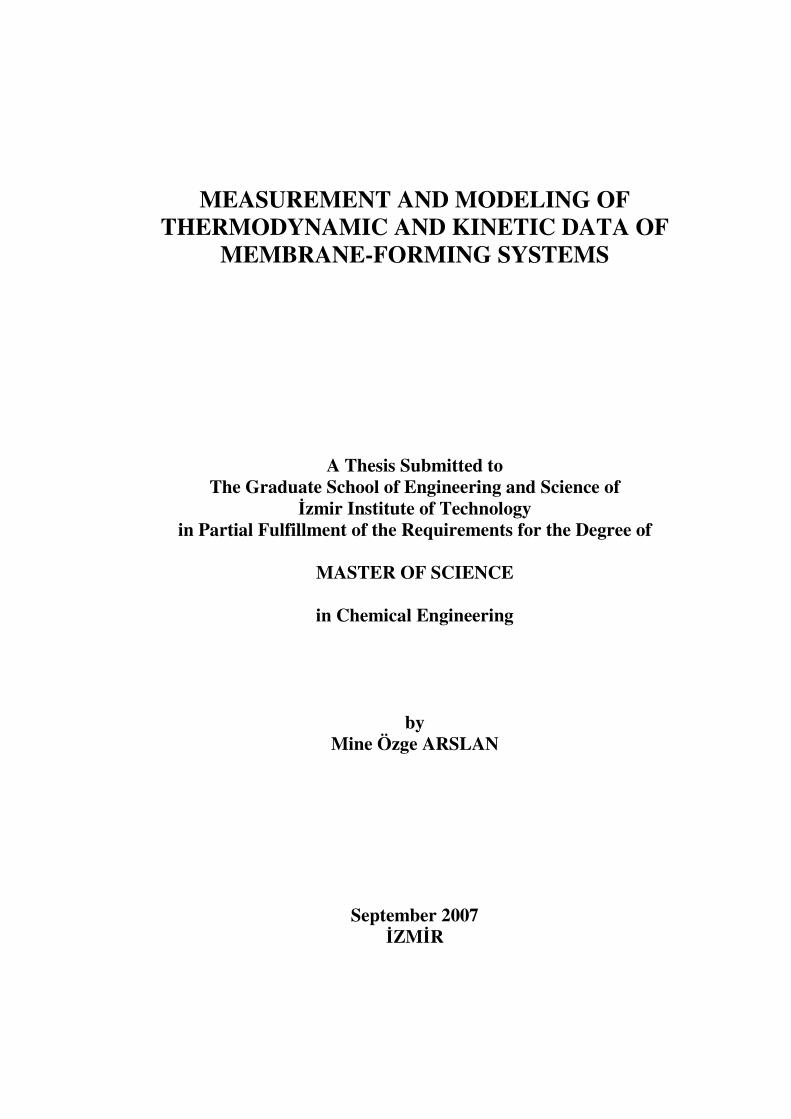
Figure 5.8. Approximate situation of the liquid-liquid (l-l) phase

separataion gap in PSf/solvent/water membrane forming

systems...................................................................................................... 45

Figure 5.9. Cloud point data for PSf-NMP-water and PSf-(NMP+PA)-

water system (� NMP; � NMP+PA) ..................................................... 45

Figure 5.10. Comparison between the calculated and experimental binodal

curves for PMMA/acetone/water system at 25°C..................................... 46

Figure 6.1. Typical sorption kinetics: (a) Fickian; (b) Two-stage;

(c) Sigmoidal; (d) Case II ......................................................................... 48

Figure 6.2. Calculation of sorption curves for different β values ............................... 55

Figure 7.1. Schematic representation of film preparation procedure .......................... 60

Figure 7.2. Fast-acting thermostated bath ................................................................... 62

Figure 7.3. Digital photograph of experimental set-up in laboratory. 1,

balance; 2, sorption cell; 3, circulating water bath; 4, water

bath; 5, pressure transducer; 6, vacuum pump; 7, cold trap; 8,

heating tape; 9, temperature controller; 10, control unit; 11,

computer ................................................................................................... 63

xii

Figure 7.4. Double walled jacket for thermostating measuring cell with a

circulating fluid......................................................................................... 64

Figure 7.5. Illustration of suspension control and balance indicator units.................. 65

Figure 7.6. Typical computer software output obtained from sorption

experiment ................................................................................................ 66

Figure 7.7. Schematic representation of the experimental system. 1,

circulating liquid thermostat; 2, balance; 3, magnetic

suspension coupling; 4, sorption cell; 5, pressure transducer; 6,

water bath including solvent flask; 7, cold trap; 8, vacuum

pump ......................................................................................................... 67

Figure 7.8. Forces affecting on the system ................................................................. 68

Figure 7.9. Explanation of the system ........................................................................ 70

Figure 8.1. SEM picture of the cross section of polysulfone film used to

measure film thickness.............................................................................. 72

Figure 8.2. Differential Scanning Calorimetry analysis of polysulfone film.............. 73

Figure 8.3. Thermal Gravimetric Analysis of polysulfone film.................................. 74

Figure 8.4. Comparison of experimental cloud point curves for

PSf/THF/Water system ............................................................................. 75

Figure 8.5. Comparison of experimental cloud point curves for

PSf/NMP/Water system............................................................................ 75

Figure 8.6. Experimental cloud points for Polysulfone/Solvent/Water

system ....................................................................................................... 76

Figure 8.7. Experimental cloud points for Polysulfone/Solvent/Ethanol

system ....................................................................................................... 77

Figure 8.8. Experimental cloud points for PMMA/Solvent/Water system ................. 77

Figure 8.9. Experimental cloud points for PMMA/Solvent/Formamide

system ....................................................................................................... 78

Figure 8.10. Experimental cloud points for PSf/NMP/Nonsolvent system .................. 79

Figure 8.11. Experimental cloud points for PSf/THF/Nonsolvent system ................... 79

Figure 8.12. Experimental cloud points for PMMA/Acetone/Nonsolvent

system ....................................................................................................... 80

Figure 8.13. Experimental cloud points for PMMA/THF/Nonsolvent system ............. 80

Figure 8.14. Effect of temperature on the experimental cloud points for

PSf/THF/Water system ............................................................................. 81

xiii

Figure 8.15. Comparison of theoretical binodal curves with experimental

cloud points for PSf/NMP/water system .................................................. 83


cloud points for PSf/THF/water system.................................................... 83


cloud points for PSf/NMP/ethanol system................................................ 84


cloud points for PSf/THF/ethanol system................................................. 84


cloud points for PMMA/acetone/water system ........................................ 85


cloud points for PMMA/THF/water system ............................................. 85


cloud points for PMMA/THF/formamide system .................................... 86

Figure 8.22. Normalized mass uptakes for the diffusion of water in

polysulfone at 30°C. The solid line represents the the

theoretical Fickian curve and the symbol represents the

experimental sorption curve. Water vapor temperatures:

a) 14°C, b) 18°C, c) 22°C, d) 26°C .......................................................... 87





a) 20°C, b) 25°C, c) 30°C, d) 35°C .......................................................... 90





a) 20°C, b) 25°C, c) 30°C, d) 35°C, e) 40°C, f) 45°C .............................. 92

Figure 8.25. Diffusion coefficients of water in the polysulfone films as a

function of its average weight fraction for 3 sets of repeated

experiments at 50°C.................................................................................. 96

xiv

Figure 8.26. Comparison of the diffusion coefficients with the study of

Schult and Paul (1996a). Regain is the weight of the water

sorbed at the given activity by the dry weight of the polymer. ................ 97

Figure 8.27. Bouyancy corrected weight difference values as a function of

t for the diffusion of chloroform in polysulfone at 30°C. The

solid line represents the theoretical curve and the symbol

represents the experimental sorption curve. Water vapor

temperatures: a) 9.9°C, b) 14°C, c) 18°C ................................................. 98


t for the diffusion of chloroform in polysulfone at 40°C. The

solid line represents the the theoretical curve and the symbol

represents the experimental sorption curve. Chloroform vapor

temperatures: a) 11.5°C, b) 25°C, c) 30.8°C, d) 36°C............................ 100

Figure 8.29. Plot of Tg as a function of volume fraction of solvent............................ 105


t for the diffusion of ethanol in polysulfone at 30°C of Set 2.

The solid line represents the the theoretical curve and the

symbol represents the experimental sorption curve. Ethanol

vapor temperatures: a) 11.9°C, b) 20°C, c) 25.6°C ................................ 106


t for the diffusion of ethanol in polysulfone at 40°C of Set 2.

The solid line represents the the theoretical curve and the

symbol represents the experimental sorption curve. Ethanol

vapor temperatures: a) 11.2°C, b) 16.2°C, c) 20.1°C, d) 30.2°C,

e) 35°C .................................................................................................... 108


t for the diffusion of ethanol in polysulfone at 30°C for Set

1. The solid line represents model predictions and the symbol

represents the experimental sorption curve. Ethanol vapor

temperatures: a) 11.7°C, b) for 15.9°C, c) 20.1°C, d) 25.1°C ............... 112

xv


t for the diffusion of ethanol in polysulfone at 40°C for Set

1. The solid line represents model predictions and the symbol

represents the experimental sorption curve. Ethanol vapor

temperatures: a) 14.3°C, b) 25°C, c) 30°C, d) 35°C............................... 114

Figure 8.34. Plot of Mt/M∞ as a function of Lt at activity = 0.33 for

different thicknesses ............................................................................... 117





Figure 8.37. Sorption isotherms for 3 sets of repeated experiments at 50°C.............. 120

Figure 8.38. Sorption isotherm of water-polysulfone system ..................................... 122

Figure 8.39. Sorption isotherm of chloroform-polysulfone system............................ 123

Figure 8.40. Sorption isotherm of ethanol-polysulfone system .................................. 124

Figure 8.41. Experimental and correlated diffusivities with respect to weight

fraction of water. The symbols represent the experimental data

while the lines correspond to the free volume correlation...................... 126

xvi

LIST OF TABLES

Table Page

Table 2.1. Membrane materials ..................................................................................... 5

Table 3.1. Group Contribution Methods to Estimate Molar Volumes at 0 K.............. 11

Table 7.1. Properties of polymers ................................................................................ 59

Table 8.1. Flory Huggins interaction parameters......................................................... 82

Table 8.2. Diffusivity data for water-polysulfone at 30°C, 40°C and 50°C................ 95

Table 8.3. Diffusivity data for chloroform-polysulfone at 30°C and 40°C ............... 102

Table 8.4. Deborah numbers, τR and α values for chloroform-PSf at 30°C

and 40°C .................................................................................................. 103

Table 8.5 Diffusivity data for ethanol-polysulfone at 30°C and 40°C for

Set 2 .......................................................................................................... 110

Table 8.6. Diffusivity data for ethanol-polysulfone at 30°C and 40°C of Set 1 ............ 116

Table 8.7 Deborah numbers, τR and α values for ethanol-polysulfone at

30°C and 40°C ......................................................................................... 116

Table 8.8. Diffusion coefficients of ethanol in PSf as a function of the film

thickness.................................................................................................... 118

Table 8.9. Sorption isotherms for water in polysulfone measured at the

column temperatures 30°C, 40°C and 50°C ............................................. 119

Table 8.10. Sorption isotherms for chloroform in polysulfone measured at

the column temperatures 30°C and 40°C.................................................. 120

Table 8.11. Sorption isotherms for ethanol in polysulfone measured at the

column temperatures 30°C and 40°C ....................................................... 121

Table 8.12. Free volume parameters of polysulfone and water ................................... 125

xvii

LIST OF SYMBOLS

V* Minimum hole size into which molecule can jump

Vf The average hole free volume per sphere

A The proportionality constant

γ The overlap factor to account for the overlap between free volume elements

D1 Solvent self diffusion coefficient in a polymer solution (cm2/s)

D0 Constant preexponential factor

D Mutual diffusion coefficient (cm2/s)

E Activation energy per mole that a molecule needs to overcome attractive

forces holding it to its neighbors (J/mole.K)

∗iV̂ Specific critical hole free volume required for a diffusive jump of the

component i (cm3/g)

R Universal gas constant (cal/mol.K)

FHV̂ Specific hole free volume of the polymer-solvent mixture (cm3/g)

Tgi Glass transition temperature of component i (K)

Q Thermodynamic factor

∗1̂V , ∗

2V̂ Specific volumes of the solvent and polymer at 0 K (cm3/mol)

K11 Solvent free volume parameter (cm3/g.K)

K21 Solvent free volume parameter (K)

K12 Polymer free volume parameter (cm3/g.K)

K22 Polymer free volume parameter (K) WLFC12 , WLFC22 WLF constants

at Shift factor

G′ Loss modulus

G″ Storage modulus

)0(~1�V , ∗

jV2~

Solvent molar volume at 0 K and the molar volume of the polymer jumping unit

M1 Molecular weight of the solvent (g/mol)

cV~

Molar volume of the solvent at its critical temperature (cm3/mol)

1̂V Molar volume of the pure solvent (cm3/g)

P1 Vapor pressure of the solvent at T (atm)

xviii

satP1 Saturation vapor pressure of the solvent at the column temperature (atm)

∆f Crystal frequency shift

K Proportionality constant

χ13 Flory Huggins nonsolvent/polymer interaction parameter

χ23 Flory Huggins solvent/polymer interaction parameter

g12 Flory Huggins nonsolvent/solvent interaction parameter

νi Molar volume of component i

2δ , 3δ Solubility parameter of solvent and polymer (cal1/2/cm3/2)

Mt, M∞ Penetrant mass uptake at time t and at equilibrium (g)

L Film thickness (cm)

C0 Concentration of the penetrant in the polymer at time t = 0 (g/cm3)

Ceq Concentration of the penetrant at the surface at time t > 0 (g/cm3)

M∞,i Equilibrium sorption due to the ith relaxation process (g)

ki First-order relaxation constant of the ith relaxation process

αR Fraction of weight uptake controlled by polymer relaxation

τR Time constant characterizing the long time drift in mass uptake toward

equilibrium (sec)

tD Delay factor associated with a delay in the beginning of structural

relaxation (sec)

β Inverse of the characteristic time for attaining saturation at the surface

λm Relaxation time for the polymer-solvent systems

θD Characteristic diffusion time

De Deborah number

η1, η2 Viscosity of the solvent and polymer (g/cm.s)

ξ Ratio of molar volume of the solvent jumping unit to that of the polymer

jumping unit

ωi Weight fraction of the component i

φi Volume fraction of the component i

µi Chemical potential of the component i

Na, Nb Mole fraction of component a and b

ka, kb Uptake rate constants for pure liquid a or b

t Time (sec)

1

CHAPTER 1

INTRODUCTION

Polymeric membranes are widely used in pharmaceutical, chemical, biomedical,

food and biotechnology industries for different separation purposes. Several methods

are used for producing polymeric membranes, however phase inversion method

invented by Loeb and Sourirajan in 1962, is the most common method. In this method,

an initially homogeneous polymer solution thermodynamically becomes unstable due to

different external effects and phase separates into polymer lean and polymer rich

phases.

The kinetics and thermodynamics of the phase separation process have

important roles in determining the final structure of the membranes. Depending on the

evaporation/quenching conditions, initial thickness and composition of the polymer

solution, various membrane stuctures ranging from dense to highly asymmetric ones can

be obtained. Membrane preparation conditions, thus, membrane formation process and

morphology can be optimized by using reliable mathematical models which require

both thermodynamic and diffusivity data (Alsoy Altinkaya and Ozbas 2004).

Information about ternary phase diagrams describing the equilibrium behavior of liquid-

liquid phase separation is also important and needed for studying membrane formation

mechanisms (Lai et al. 1998).

Experimentally, phase diagrams are constructed using cloud point curves. The

method of titrating polymer solutions with nonsolvents is generally in use for the

determination of cloud point curves (onset of turbidity as function of composition)

(Schneider et al. 2002). The amounts of nonsolvents required to bring the onset of

turbidity are measured and at the onset of turbidity, the volume fractions of nonsolvent,

solvent and polymer represent the cloud points in a ternary phase diagram. Various

techniques have been used for the measurement of diffusivity of polymer solvent

systems such as inverse gas chromatography (IGC), pressure decay method, FTIR-ATR

spectrophotometry and sorption measurements either gravimetric or piezoelectric.

Kleinrahm and Wagner (1986) developed a unique balance, so-called a magnetic

suspension balance (MSB), which is one of the most reliable and sensitive apparatus

among other gravimetric sorption equipments such as quartz spring balance or Cahn

2

electrobalance. By using this device, the measuring force is transmitted contactlessly

from the measuring chamber to the microbalance. The weight change of the sample is

obtained in the range of micrograms as a function of time.

In this study, polysulfone (PSf) and polymethylmethacrylate (PMMA) have been

selected due to their excellent chemical resistance, mechanical strength, thermal

stability and transport properties, hence, their frequent use as membrane materials.

There are a few reports presenting the experimental phase diagrams in ternary mixtures

of PSf/solvent/water (Altena and Smolders 1982, Kim et al. 1997, Barth and Wolf

2000). The solvents studied are dimethylacetamide (DMAc), NMP, dimethylformamide

(DMF) and THF. It was observed that for all systems small amount of water is required

to achieve phase separation due to hydrophobic nature of PSf. Lai et al. (1998)

constructed the ternary phase diagrams of PMMA/acetone/water, PMMA/n-butyl

acetate/n-hexane and PMMA/acetone/n-hexane systems at 25°C. Kinetic studies for

PSf/solvent or PSf/nonsolvent pairs are very limited. Only in a few studies, diffusivities

and sorption isotherms of water in polysulfone were measured (Swinyard et al. 1990,

Schult and Paul 1996a, Schult and Paul 1996b, Karimi et al. 2005).

The main objective of this study is to collect thermodynamic and kinetic data for

two most commonly used membrane forming materials, PSf and PMMA. For this

purpose, the diffusivity and equilibrium isotherms of water, ethanol and chloroform in

PSf were determined by using a magnetic suspension balance. In addition, experimental

cloud points of PSf/NMP (1-methyl-2-pyrrolidinone)/water, PSf/THF

(Tetrahydrofuran)/water, PSf/NMP/ethanol, PSf/THF/water, PMMA

(Polymethylmethacrylate)/acetone/water, PMMA/THF/water, PMMA/acetone

/formamide and PMMA/THF/formamide systems were determined by the titration of

homogeneous polymer solutions (8-22 w%) with nonsolvents until the onset of

turbidity. Theoretically, binodal curves were calculated by using nonsolvent/polymer

(χ13), solvent/polymer (χ23) and nonsolvent/solvent (χ12) interaction parameters and

agreement between experimental cloud points and theoretical binodal curves were

investigated. A correlation that describes diffusivity of water in polysulfone as a

function of temperature and concentration was obtained by using Vrentas and Duda free

volume theory and all equilibrium isotherms were correlated by Flory Huggins theory

(Flory 1953).

This thesis consists of nine sections. After giving a brief introduction in the first

part, in the second part, information about membrane materials are given. Free volume

3

theory, sorption isotherms and previous diffusion and equilibrium studies on

polysulfone are reviewed in the third section. Methods developed for the measurement

of diffusivities in polymer-solvent systems are discussed in the fourth section while

methods for measurement of cloud point curves and construction of ternary phase

diagrams are given in the fifth section. In the sixth section, information about modeling

process are reviewed. Materials and methods are given in seventh section, while in the

eighth section, results are shown and discussed. Finally in the ninth section, conclusions

are given.

4

CHAPTER 2

MEMBRANE MATERIALS AND PROPERTIES

Sorption and diffusion data are related to a variety of applications including

membrane separation of gases and vapors; packaging and coating technology;

controlled drug release systems, and materials for biomedical applications (Rodriguez et

al. 2003). Typical membrane applications are microfiltration, ultrafiltration, gas

permeation and dialysis. Each application needs specific requirements on the membrane

material (van de Witte 1996).

In order to use membranes in these applications, some requirements are needed

for membrane materials. The most important membrane material requirements are high

selectivity, high permeability, mechanical strength, temperature stability and chemical

resistance (Rautenbach and Albrecht 1989).

Membrane materials can be classified as “modified natural products” and

“synthetic products”. Modified natural products are cellulose derivatives such as

cellulose acetate, cellulose acetobutyrate, cellulose nitrate etc. Polyamide,

polymethylmethacrylate (PMMA), polysulfone, polyfuran, polycarbonate, polyethylene,

polypropylene and polyethersulfone can be given as examples for synthetic products.

Commercial membranes are usually produced from polymers due to their low cost and

performance. However, ceramic membranes are prefered in case of high temperature

applications due to their thermal stability at higher temperatures. Typical materials used

in membrane fabrication are shown in Table 1. Among these materials, polysulfone and

polymethylmethacrylate are widely used as membrane materials.

5

Table 2.1. Membrane materials

(Source: Rautenbach and Albrecht 1989)

Modified natural products Cellulose acetate (cellulose-2-acetate, cellulose-2,5-diacetate, cellulose-3-acetate), cellulose acetobutyrate, cellulose regenerate, cellulose nitrate Synthetic products Polyamide (aromatic polyamide, copolyamide, polyamide hydrazide), polybenzimidazole, polysulfone, vinyl polymers, polyfuran, polycarbonate, polyethylene, polypropylene, PVA, PAN, polyethersulfone, polyolefins, polyhydantoin, (cyclic polyurea), polymethylmethacrylate Miscellaneous Polyelectrolyte complex, porous glass, graphite oxide, ZrO2-polyacrylic acid, ZrO2-carbon, oils, Al2O3

2.1. Polysulfone Based Membranes

According to their chemical, mechanical, thermal, hydrolytic stability and

excelllent insulative capabilities, polysulfones are of practical interest as membrane

materials (Tweddle et al. 1983). Polysulfone is a high performance polymer used for

numerous applications across the membrane separation processes. Polysulfone films

have the advantage of applicability to a wide range of pH and temperature (O�uzer

2004). Polysulfones also have high permeability and permselectivity that make them

attractive as membrane polymers in gas separation (Fried 1995). The inert and sulfone

backbone functionalities supply resistance against hydrolysis and chemical attack by

acid and bases. This characteristic feature makes polysulfone valuable in medical and

food contact applications. Polysulfone membranes are used in ultrafiltration, reverse

osmosis and hemodialysis (artificial kidney) units. Gas separation membrane

technology was developed in the 1970s based on polysulfone hollow-fiber membranes

(Mark 2004). There are several examples for the commercial use of polysulfone in gas

permeation processes such as separating CO2-CH4 and recovery of H2 (Rautenbach and

Albrecht 1989). Polysulfone-based membranes are also used recently for plazma

separation from blood (WEB_1 2007). Some physical and chemical properties of

polysulfone are given in Table 7.2.

Polysulfones are characterized by the presence of the para-linked

diphenylenesulfone group as part of their backbone repeat units (Mark 2004).

Polysulfone repeat unit is given in Figure 2.1.

6

Figure 2.1. Polysulfone molecular structure

(Source: WEB_2 2007)

2.2. PMMA Based Membranes

PMMA is an amorphous polymer with high light transparency and good

resistance to acid and environmental deterioration (Fried 1995). PMMA is used in

contact lenses. The successful lens product must provide appropriate water content and

oxygen permeability. Comport and on-eye movement depend on water content and

water transport properties (Rodriguez et al. 2003). Among the variety of polymeric

membranes for gas separation, PMMA possess high solubility in a large number of

organic solvents. Many researchers have studied PMMA to elucidate how the casting

solvent affect the performance of the gas separation membrane (Tung et al. 2006).

The repeated unit of PMMA is given in Figure 2.2, while its physical and

chemical properties are given in Table 7.2.

Figure 2.2. PMMA molecular structure


7

CHAPTER 3

DIFFUSION AND THERMODYNAMIC BEHAVIOR OF

POLYMER/SOLVENT MIXTURES

By the invention of the phase inversion technique, it became the most popular

method to prepare asymmetric polymeric membranes. Asymmetric membranes consist

of a very thin dense layer and a porous sublayer. The permeability and high selectivity

is provided by the dense layer while the mechanical strength is imparted by the porous

sublayer. According to the desired application and operating costs, structural

characteristics of the membrane can be adjusted by optimizing the membrane

preparation conditions. Prediction of membrane formation mechanisms and morphology

can overwhelm time consuming trial and error experimentation (Alsoy Altinkaya and

Ozbas 2004).

The polymer rich phase forms the matrix of the membrane, while, the polymer

lean phase, rich in solvents and nonsolvents, fills the pores. After the polymer solidifies,

the liquid in the pores is extracted. The phase inversion techniques can be classified into

four groups based on the external effects: immersion precipitation (wet-casting), vapor-

induced phase separation, thermally induced phase separation and dry-casting (Ozbas

2001).

3.1. Prediction of Diffusivities of Small Molecules in Polymers

3.1.1. Free Volume Theory

Free volume theory was first introduced by Cohen and Turnbull in 1954.

According to Cohen and Turnbull, the small molecules are assumed as hard spheres,

and if one of the spheres moves to another direction and leaves a space behind it,

another sphere may jump to this vacancy. A molecule is able to move if the following

two conditions are fulfilled: (1) a sufficiently large hole opens up next to the molecule

due to a fluctuation in local density, and (2) the molecule has sufficient energy to break

away from its neighbors. Such displacements result in diffusive motion. However, the

8

diffusional transport will be completed only if another molecule jumps into the hole

before the first molecule returns to its initial position. Hence, the diffusion constant can

be related to the average number of jumps per unit time and the jump distance.

According to this theory, diffusion coefficient is proportional to the probability of

finding a hole that is sufficiently large for the molecule. The following equation shows

the relationship between self diffusion and free volume (Cohen and Turnbull 1954).

(3.1)

where V* is the minimum hole size into which molecule can jump, Vf is the average

hole free volume per sphere, the proportionality constant A is related to the gas kinetic

velocity and γ is the overlap factor to account for the overlap between free volume

elements.

Many researchers have extended Cohen and Turnbull’s free volume theory to

describe molecular transport in polymer solutions. Among these studies, the most

successful one was derived by Vrentas and Duda (1977).

3.1.2. Vrentas Duda Free Volume Theory

In Vrentas Duda free volume theory, total volume of the liquids is divided into

two parts: occupied volume which is taken by the molecules themselves and free volume

between the molecules. Total free volume also consists of two parts: hole free volume

and interstitial free volume. When two molecules come close to each other, the

repulsive forces can not be negligible, so the free volume within a system is not

accessible for molecular transport. Due to usual random thermal fluctuations, some of

this free volume is continuously being redistributed and is called as hole free volume

where molecular transport takes place in this part of the free volume. The remaining

part of the free volume, which is not being continuously redistributed is called

interstitial free volume and is not available for molecular migration. The specific

volume/temperature relationship was given in Figure 3.1.

��

��

�−×= fVV

AD*

1 expγ

9

Figure 3.1. Vrentas Duda concept of free volume of a polymer above and below the

glass transition temperature Tg (Source: Mohammadi 2005)

Vrentas and Duda extended this theory to binary polymer-solvent systems and

derived the following expression for solvent self diffusion coefficient in a polymer

solution, D1:

(3.2)

Here D0 is a constant preexponential factor, E is the activation energy per mole

that a molecule needs to overcome attractive forces holding it to its neighbors

(J/moleK), ∗iV̂ is the specific critical hole free volume required for a diffusive jump of

the component i, R is the universal gas constant, γ is an overlap factor, and ωi is the

weight fraction of the component i. In Equation (3.2), FHV̂ is the specific hole free

volume of the polymer-solvent mixture given by:

( )��

�

�

��

�

�

+−×��

��

�−=∗∗

γ

ξωω

FHVVV

RTE

DD ˆˆˆ

expexp 221101

10

(3.3)

where K1i and K2i are free volume parameters and Tgi is the glass transition temperature

of component i.

Incorporating the work of Bearman (1961), following relationship to express the

mutual diffusion coefficient, D by the self diffusion coefficient is proposed by Duda et

al. (1982):

(3.4)

where Q is the thermodynamic factor and is defined as:

(3.5)

If chemical potential is calculated from a modified version of the Flory Huggins

equation which includes concentration dependent χ parameter

(3.6)

then Equation (3.5) is rewritten as follows:

(3.7)

For a constant interaction parameter, combining Equation (3.4) and (3.5) leads to

the following equation which is the most widely used form of the mutual diffusion

coefficient

(3.8)

Then, the expression for the mutual diffusion coefficient become

)()(ˆ222122121111 TTKKTTKKV ggFH +−++−= ωω

QDD 1=

PTRT

Q,1

121��

�

�

∂∂=ωµωω

( ) ( ) ��

��

�−+−=

11211

22 221

φχφφφχφφ

dd

Q

( )1221 21 χφφ −= DD

1

221

22211

011 lnln

φχφφχφφφµµ

dd

aRT

+++==−

11

(3.9)

3.1.2.1. Estimation of Free Volume Parameters

There are 13 independent parameters to be evaluated in Equation (3.9).

Grouping some of them means that only 10 parameters need to be determined to

estimate the mutual diffusion coefficients. The free volume parameters can be estimated

if chemical structure of both solvents and polymers, viscosity of each pure component at

different temperatures, critical molar volume of the solvents and glass transition

temperature of the polymer are known.

∗1̂V and ∗

2V̂

The two critical volumes, ∗1̂V and ∗

2V̂ are the specific volumes of the solvent and

polymer at 0 K. Molar volumes at 0 K can be estimated by using group contribution

methods developed by Sugden (1927) and Biltz. Haward (1970) has summarized these

methods, and a corrected version of his summary is presented in Table 3.1.

Table 3.1. Group Contribution Methods to Estimate Molar Volumes at 0 K

(Source: Hong 1995)

Component Sugden (cm3/mol) Biltz (cm3/mol) H 6.7 6.45 C (aliphatic) 1.1 0.77 C (aromatic) 1.1 5.1 N 3.6 N (in ammonia) 0.9 O 5.9 O (in alcohol) 3.0 F 10.3 Cl 19.3 16.3 Br 22.1 19.2 I 28.3 24.5 P 12.7 S 14.3

(cont. on next page)

( )( ) ( )��

��

�

�

�

+−��

�

�++−��

�

�

+−��

�

� −=∗∗

TTKK

TTKK

VVRT

EDD

gg 22212

212111

1

221101

ˆˆexpexp

γω

γω

ξωω

12

Table 3.1. (cont.) Triple bond 13.9 16.0 Double bond 8.0 8.6 3-membered ring 4.5 4-membered ring 3.2 5-membered ring 1.8 6-membered ring 0.6 OH (alcoholic) 10.5 OOH (carboxyl) 23.2

γ/11K and 121 gTK − (Solvent free volume parameters)

An empirical equation to describe the viscosity-temperature relationship was

proposed by Vogel in 1921. Doolittle then, described that viscosity should be related to

the amount of free volume in a system and derived the equation of Vogel in terms of

free volume concepts (Doolittle 1951). The relationship between the viscosity of the

solvent, η1 and the free volume parameters are given by the following equation (Hong

1995).

(3.10)

where A is a constant. Hence, γ/11K and 121 gTK − can be determined from a nonlinear

regression of Equation (3.10) using viscosity-temperature data.

γ/12K and 222 gTK − (Polymer free volume parameters)

The free volume parameters of polymer can also be evaluated from the nonlinear

regression of Doolittle’s expression if the viscosity of the polymer is measured at glass

transition temperature and 100°C above the Tg. However, viscosity data near the glassy

region are generally not available. An alternate form of the Doolittle expression is

developed by William, Landel and Ferry which is a commonly used relationship in

correlating viscosity with temperature for pure polymers as shown in Equation (3.11).

(3.11)

TTKKV

Ag +−

+=∗

)()/ˆ(

lnln121

11111

γη

TTC

TTC

TT

gWLF

gWLF

g +−−−

=��

�

�

�

222

)212

22

2(

)()(

logηη

13

where η2 is the viscosity of the polymer and WLFC12 , WLFC22 are the WLF constants. The

free volume parameters for polymer are obtained from WLF constants as follows (Hong

1995):

(3.12)

(3.13)

Values of WLFC12 and WLFC22 for a large number of polymers have been published

by Ferry (1970). When these constants are not available for the polymer of interest, they

can be obtained from experimental measurements of shift factor, at. The proper

relationship between the shift factor and the temperature can be obtained by measuring

loss modulus, G′; and storage modulus, G″ as a function of frequency at several

temperatures. Master curve is obtained from loss modulus and storage modulus as a

function of temperature of ω (rad/s) and shift factor can be obtained by shifting the data

until they overlap. The relationship between the shift factor and the temperature in terms

of WLF constants are given by the following equation:

(3.14)

ξ, D0 and E

The parameter ξ is the ratio of molar volume of the solvent jumping unit to that

of the polymer jumping unit. Binary experimental diffusivity data are the correlation

source for D0, ξ and E. These free volume parameters can be evaluated from the

experimental diffusion data by nonlinear regression analysis. These parameters can also

be predicted if no diffusivity data are available. Assuming that solvent molecule moves

as a single unit, then it may be expressed as:

(3.15)

WLFCK 2222 =

WLFWLF CCVK

2212

212

303.2

ˆ ∗

=γ

ref

refT TTC

TTCa

−+−

−=22

12 )(log

jj MVMV

VV

22

11

2

1

ˆˆ

~)0(

~

∗

∗

∗ ==�

ξ

14

where )0(~

1�V and ∗

jV2~

are the solvent molar volume at 0 K and the molar volume of the

polymer jumping unit, respectively. M1 and M2j are the molecular weights of the solvent

and the polymer jumping unit, respectively. Zielinski (1992) assumed that the size of

the polymer jumping unit is independent of the solvent and proposed a linear

relationship between ξ and the solvent molar volume at 0 K as given by the Equation

(3.16):

(3.16)

where β is a constant. According to this relationship, once β is known for a specific

polymer the ξ parameter for any solvent in a polymer can be determined. β values have

been reported for various polymers (Ju et al. 1981a, Ju et al. 1981b).

In addition, D0 and E can be estimated by combining the Dullien equation

(Dullien 1972) for the self diffusion coefficient of pure solvents with the Vrentas Duda

free volume equation in the limit of pure solvents (Hong 1995).

(3.17)

where cV~

(cm3/mol) is the molar volume of the solvent at its critical temperature, 0.124

× 10-16 is a constant and η1 (g/cm.s) and 1̂V (cm3/g) are the viscosity and the molar

volume of the pure solvent, respectively, and are the only temperature dependent

parameters in the expression. Since solvent free-volume parameters have been

determined previously from Equation (3.10), D0 and E can be determined from the

nonlinear regression (Hong 1995). According to Equation (3.17), D0 is a solvent

property and independent of the polymer.

3.2. Prediction of Sorption Isotherms of Polymer/Solvent Systems

The dependence of penetrant concentration on the penetrant pressure is

described by a sorption isotherm. There are four general isotherms that describe

)0(~ˆ

112

2 �VKV βξγ =

∗

( )TTK

KV

RTE

DVM

RTV

g

c

+−−→−=��

�

�

� ×

∗

−

121

11

1

10

111

3/216

ˆ

1ln~

~10124.0

ln

γω

η

15

sorption of small molecules in a polymer matrix as shown in Figure 3.2. These

isotherms are known as the (a) Henry’s Law, (b) Dual Mode, (c) Flory Huggins, and (d)

Generalized isotherms. Among these isotherms, Flory Huggins theory has been

successfully used to correlate sorption isotherms of polymer/solvent systems.

Figure 3.2. Sorption isotherms of vapors in polymers

(Source: McDowell 1998)

During a typical sorption experiment, when the penetrant vapor reaches an

equilibrium with the polymer, then

(3.18)

If vapor pressure of the polymer is neglected and ideal gas of pure solvent is

assumed, then activity of the penetrant is calculated as follows:

polymerpenetrant

vaporpenetrant µµ =

16

(3.19)

where P1 is the pressure of the solvent measured and satP1 is the saturation vapor

pressure of the solvent at the column temperature. If the interaction parameter χ is

constant, then, Equation (3.6) combined with Equation (3.19) is written as follows:

(3.20)

χ parameter is regressed from Equation (3.20) by minimizing the difference

between the experimental and theoretical activity data. Experimental data usually

collected as the weight fraction of penetrant is converted into volume fraction through

following expressions:

(3.21)

where subscripts 1 and 2 refer to penetrant and polymer, respectively.

The strength of the polymer-penetrant interaction is characterized by the

magnitude of Flory-Huggins parameter. The correlation between the solvation power of

a penetrant in a given polymer and χ has been given as follows (Feng 2001):

1. if χ < 0, there is strong interaction between polymer and penetrant, water will

not cluster

2. if χ is between 0 and 0.5, it is a good solvent for that polymer

3. if χ is greater than 0.5, penetrant can not completely dissolve the polymer

4. if χ > 1, water tends to cluster

satPP

a1

11 =

22210

1

1 lnln χφφφ ++=PP

2211

111 ˆˆ

ˆ

VVVωω

ωφ+

=

17

3.3. Previous Diffusion and Equilibrium Studies with Polysulfone

Schult and Paul (1996a) have measured diffusion coefficients of water in

polysulfone at 30, 40 and 50°C. The diffusion coefficients were obtained as 9.5 × 10-8 at

activity equals to 0.5 and 8.9 × 10-8 at activity 1 (Figure 3.3).

Figure 3.3. Diffusion coefficients for the various polysulfones at 40°C calculated from

the sorption kinetic data plotted versus (a) average water activity and (b)

average water concentration (Source: Schult and Paul 1996a)

They have also measured equilibrium isotherms were at 30°C, 40°C and 50°C.

Figure 3.4 shows the equilibrium isotherm at 40°C. The isotherms were represented in

terms of the weight of water sorbed by the film at a given water vapor activity divided

by the dry weight of the polymer.

A Cahn balance was used to measure both the equilibrium and the kinetics of

water vapor sorption. The initial slope method was used to determine the diffusion

coefficients from sorption data. Authors claimed that Fickian sorption kinetics with a

mildly concentration-dependent diffusion coefficient was obtained. It was observed that

at low activities diffusion coefficients of water in PSf increase with activity, and

decreases at high activitities. Such decrease at high activity was attributed to self-

hydrogen bonding of water molecules to form clusters and clustering became more

pronounced at activities above 0.5.

18

Figure 3.4. Equilibrium water vapor isotherms for polysulfones at 40°C. Water

concentration was measured in terms of the regain, which is the weight of

the water sorbed at the given activity divided by the dry weight of the

polymer (Source: Schult and Paul 1996a)

In the study of Karimi et al. (2005), sorption isotherms of water in polysulfone

were determined at 25°C by use of magnetic suspension balance. It is observed that in

the water activity range of 0.20-0.95, the water uptake is linear with water vapor

pressure.

Figure 3.5. Sorption isotherms for water in CA, PES, PEI and PSU at 25°C. The curves

represent fits with the Flory Huggins theory (Source: Karimi et al. 2005).

19

CHAPTER 4

METHODS DEVELOPED FOR THE MEASUREMENT OF

DIFFUSIVITIES IN POLYMER-SOLVENT SYSTEMS

Various techniques have been used for the measurement of diffusivity of

polymer solvent systems such as inverse gas chromatography (IGC), pressure decay

method, FTIR-ATR spectrometry and sorption measurements either gravimetric or

piezoelectric.

4.1. Inverse Gas Chromatography (IGC)

Inverse gas chromatography has been used to study sorption and diffusion in

polymer-solvent systems accurately (Surana et al. 1996, Tihminlioglu et al. 2000,

Balashova et al. 2001, Davis et al. 2004a). Gray and Guillet (1973) are the first

researchers developing gas chromatography for the diffusion measurements by the IGC

method. In a typical IGC experiment, a polymeric stationary phase is placed inside an

empty column. The polymeric stationary phase can be in the form of a capillary column

or packed column. In capillary column inverse gas chromatography (CCIGC), inside of

a capillary column is coated with a thin film of polymer while in packed column inverse

gas chromatography (PCIGC), the polymer is coated on support particles and these

coated particles are then packed into the column. The first IGC studies done for

measuring diffusion coefficients of penetrates in polymers used packed columns. A new

mathematical model was proposed by Romdhane and Danner (Romdhane 1994) for

describing the chromatographic process in packed columns. Because of the difficulties

in knowing the geometry and morphology of the stationary phase, some problems had

been observed in getting reliable diffusion data. The morphology of the stationary phase

can differ according to the nature of the polymer and the amount of polymer needed for

preparing the column. These problems were solved with capillary columns with a

uniformly distributed polymeric stationary phase by Pawlisch et al (1987). However, the

preparations of such uniform morphology in capillary columns present some difficulties

in elastomeric polymers or polymers with low glass transition temperature.

20

The principle of IGC method is based on to measure the residence time of a

volatile solvent in the carrier gas (mobile phase) dissolving and passing the polymer

(stationary phase) inside a GC column (Krüger et al. 2006). A pulse of solvent is

injected and vaporized into the column by a carrier gas flowing through the column.

Due to the mass transfer resistance in the polymer phase, the solute is swept through the

column. The concentration front traveling down the packed column is then measured by

a detector. The data collected are the solvent concentration in the carrier gas at the

column’s outlet as a function of time. The shape of the elution profile reflects the

properties of the polymer-solvent system. The fundamental property measured by IGC

from which most of these properties are derived is known as the retention volume, a

parameter that gives information about the thermodynamics of a polymer-solvent

system. IGC allows us to calculate thermodynamic magnitudes such as partition or

activity coefficients and the Flory-Huggins interaction parameter. Figure 4.1 shows the

experimental set-up for a capillary column inverse gas chromatography experiment

(Tihminlioglu and Danner 2000). IGC is a very fast, accurate and reliable technique,

however diffusion coefficients measured by this method is not precise because it is

difficult to ensure a constant coating thickness within the IGC column (Krüger et al.

2006). This is the case when preparing the column by handwork but this problem is

eliminated when columns are prepared by corporations.

IGC is commonly used for measurements at infinite solvent dilution. This is

achieved by injecting a very small amount (<1 µL) of solvent into a stream of an inert

gas (Danner and High, 1993). In the past, this technique has been limited to

measurements in the infinite dilution region but it has been extended to measure

diffusion coefficients at the finite concentration region. (Tihminlioglu and Danner

2000). This is achieved by doping the carrier gas with a solvent by passing the carrier

gas through a saturator maintained at constant temperature. The disadvantage of IGC is

the limitation of solvent concentration. The data show deviations in the finite

concentration because of baseline fluctuations arising from the presence of solvent in

the carrier gas. The baseline fluctuations are large, making results questionable at high

activities (Tihminlioglu and Danner 2000).

21

Figure 4.1. Experimental Set-up of IGC System

(Source: Tihminlioglu and Danner 2000)

4.2. Piezoelectric Crystal

Quartz crystal resonators are easy and precise tool for determining the weight of

the thin films. When a thin film is cast onto one of the electrodes of a thickness-shear

resonator, its acoustical resonance frequencies change due to the weight of the film.

Piezoelectric method allows the detection as little as 10 nanograms of solvent using a 10

MHz crystal (Saby-Dubreuil 2001). It operates by using the frequency response of a

quartz crystal to measure the weight of solvent captured on the polymer. Sensing is

achieved by correlating acoustic wave-propagation variations to the amount of solvent

captured at the surface. This sensor using acoustic waves was first introduced by King

in 1964. After extensive researches, the quartz crystal has been known as a sensitive

mass detecting device (Chang et al. 2000).

Figure 4.2 illustrates the experimental set-up of piezoelectric crystal sorption

system. First, the polymer film cast onto the quartz crystal resonator is located inside a

vacuum chamber. Then, the chamber is connected through electronic valves to a solvent

reservoir in which the solvent vapor pressure is equal to the saturated vapor pressure of

pure solvent. Experiments are carried out with slow ramps of increasing pressure. The

22

pressure step changes are chosen small enough to allow diffusion equilibrium at all

times. Finally, frequency is recorded as a function of time.

Figure 4.2. Experimental set-up of piezoelectric crystal sorption system

(Source: Saby-Dubreuil et al. 2001)

According to Sauerbery equation, the linear relationship between the mass

uptake (∆m) on the coated crystal and the quartz crystal frequency shift (∆f) is described

below:

(4.1)

Here, K is the proportionality constant, corresponds to known properties of the

quartz crystal. Two characteristic frequency shifts are measured for determining

sorption levels in thin polymer films. The first is the frequency shift associated with the

mass of polymer deposited on the crystal, ∆fpolymer. The second is the incremental

frequency shift resulting from the sorption of vapor at any specific pressure or activity,

∆fsorption. Using these characteristic values, the weight fraction of the sorbed vapor can

be determined from the following relationship:

(4.2)

The weight fraction can be converted into volume fractions with known

properties of the polymer and vapor (Zhang et al. 2003). Although the quartz crystal

microbalance is known to be a very precise and accurate tool, in some studies the

fKm ∆=∆

polymer

sorption

polymer

sorption

f

f

m

mwt

∆∆

==%

23

obtained results were far from the theoretical ones because of the various phenomena

that affect weight determination (Dubreuil et al. 2003).

4.3. Pressure Decay Method

The pressure-decay method was first developed by Newitt and Weale in 1948

for studying the solubilities of gases in polystyrene. This method was latter improved

for diffusion measurements by Lundberg et al. in 1963 (Davis et al. 2004b). The

pressure decay experiment is carried out by isolating a polymer sample and solvent

vapor in an autoclave. As the polymer absorbs the vapor, the amount of vapor absorbed

is calculated by the pressure drop within the autoclave and is recorded as a function of

time. Schematic representation of pressure decay equipment is shown in Figure 4.3. An

equation of state is used to calculate the mass uptake from the pressure drop.

During the 1970 and 1980s, the method was extensively used to study the

sorption of gases into glassy polymers (Davis et al. 2004). The pressure decay method

was popular because the apparatus is simple and construction cost is not expensive.

However, it is difficult to operate it with molten polymers at higher temperatures

because no high-resolution sensor of pressure is available at the high temperature

condition that is high enough to melt the polymer. Also, in this method, large amount of

sample is needed, which results in long measurement times (Sato et al. 2001).

Figure 4.3. Diagram of the pressure decay instrument

(Source: Davis et al. 2004)

24

4.4. FTIR-ATR Spectrometer

Recently time-resolved FTIR (Infrared Spectroscopy with Fourier Transform) /

ATR (Attenued Total Reflection) spectroscopy has been used to examine diffusion

coefficients in polymers (Yossef et al. 2003, Baschetti et al. 2003). The FTIR-

spectroscopy is based on the property of any material absorbing light at a determined

wavelength due to its characteristic. ATR configuration is employed for mass transport

applications. This technique allows for the analysis of diffusive transport of gases and

liquids in polymeric films. Studying the diffusion of multicomponent systems, in

particular of measuring the diffusion coefficients of each component of a mixture

absorbed by a polymeric film and possibility to detect and analyze the swelling of

penetrant in the polymer during sorption are the features of this technique.

The technique is based on the observation of total reflection where there is a

penetration of the electromagnetic field in the less dense phase called “evanescent

wave”. This wave is absorbed by the film and leaves its characteristic track in the light

beam. The spectrometer records this track and yields an interferogram (intensity as a

function of time). Then it is recomputed through a Fourier transform in order to obtain

an absorption spectrum (absorbance as a function of wavelength) where one can enable

to determine the peaks of the polymer and the penetrants. Concentration of the penetrant

in the polymer and the diffusion coefficient can be easily determined from these peaks.

Figure 4.4 is a schematic representation of an FTIR-ATR experimental

arrangement. Here, the IR beam is modulated by an interferometer and enters from one

side of the ATR element. The IR radiation reflects and is absorbed at the polymer

interface of the ATR element. Then it exits from the opposite side of the ATR element

and recorded by a detector (Yossef et al. 2003).

25

Figure 4.4. Schematic of the FTIR spectrometer and ATR attachment for the

measurement of diffusion in the polymers (Source: Yossef et al. 2003).

FTIR-ATR spectroscopy is a robust, accurate and simple to use method and can

provide reliable short-time data. The technique is also relatively inexpensive in

comparison with other techniques (Yossef et al. 2003).

4.5. Gravimetric Sorption Techniques

Gravimetric sorption technique is the classical technique where a quartz spring,

an electro balance or a magnetic suspension balance is used to measure the weight

increase of a solid or non-volatile liquid sample in a solvent vapor or gas atmosphere

due to absorption of vapor or gas in the sample.

4.5.1. Cahn Electro Balance

This apparatus is built to perform vapor sorption and diffusion experiments in

polymers with a sensitivity of 0.1 µg. The sample is hanged at the balance left arm,

26

while an inert tare is suspended at the opposite arm (Figure 4.5). The polymer sample is

maintained in a constant temperature chamber and the system is evacuated. The solvent

vapor is produced by a vapor generator and is then introduced into the chamber at a

fixed pressure and temperature (Doghieri et al. 1996). The sample weight is recorded

and plotted as a function of time by a computer. Experiments are continued until a

steady state is reached. Then the sample is totally degassed and a new pressure of vapor

is introduced to the chamber to do a new experiment. The sorption experiments by a

Cahn electrobalance cover a pressure range from 0 to 1 atm and a temperature range

from 25 to 60°C (Uriarte et al. 1998). However, this experimental setup sometimes

doesn’t provide the desired activity instantaneously. This causes some difficulties in the

determination of diffusion coefficients (Alfageme et al. 1999). In addition, the accuracy

of the balance is affected by organic solvent vapors and the experiments can not be

conducted at temperatures below 60°C.

Figure 4.5. Experimental set-up of Cahn electrobalance

(Source: Doghieri et al. 1996)

4.5.2. Quartz Spring Balance

McBain spring balance is a widely used device for gravimetric sorption (Wang

et al. 1999, Kamaruddin and Korros 2000, Huang et al. 2003, Piccinini et al. 2004,

Dhoot 2004). The apparatus is based on a spring of quartz on which the polymeric

sample is suspended and immersed in the penetrant phase. As penetrant sorbs into the

27

polymer, the load on the spring increases, and the spring extends. The elongation of the

spring is monitored with a camera, directly connected to a computer and gives a

measure of the weight change of the polymer due to the sorption of penetrant. The

spring position data are converted to mass uptake values, Mt where Mt is the mass of

penetrant sorbed by the polymer at time t per unit mass of dry polymer, and diffusion

coefficients are extracted from the time dependence of Mt. A schematic diagram of this

instrument is presented in Figure 4.6.

Figure 4.6. Schematic representation of quartz spring balance

(Source: Piccinini et al. 2004)

During a typical sorption experiment in quartz spring balance, the liquid

penetrant is supplied from solvent flask and vaporized into a reservoir up to the desired

pressure. The quartz spring is suspended in a glass column and its temperature is

controlled by a water jacket through the experiment (Piccinini et al. 2004). Before

starting the experiment, sorbed water vapor is removed from the polymer by evacuating

the balance by a vacuum pump until there is no further spring displacement. Then the

sample is exposed to penetrant at desired pressure. The pressure of penetrant is

increased in a series of steps in case the sample is equilibrated after each step (Dhoot

2004). The sample elongation is observed through a CCD camera (Piccinini et al. 2004).

The quartz spring balance is classical due to its high accuracy but the time required to

reach equilibrium is too long (Huang et al. 2003). The solvent vapor requires days or

28

weeks to diffuse into the polymer and reach equilibrium due to low diffusivities of most

solvents in the polymer. The main disadvantage of this system is the direct contact

between the measuring atmosphere and the balance. The calibration of the balance can

be affected through the long time experiments. Weight fractions of solvent up to 0.75

can be used in this method but the data become very unreliable in this range, and small

fluctuations in temperature cause large swings in data (Danner and High, 1993).

4.5.3. Magnetic Suspension Balance (MSB)

Magnetic suspension balances have been widely used in a variety of applications

such as sorption measurements of vapors in polymers (Mamaliga et al. 2004, Krüger

and Sadowski 2005, Krüger et al. 2006), solubility of gases (Chaudhary and Johns 1998,

Pfannschmidt and Michaeli 1998, Schnitzler and Eggers 1999, Sato et al. 2001, Areerat

et al. 2002, Nalawade et al. 2006), adsorption measurements (Dreisbach et al. 1998,

Dreisbach and Lösch 2000, Dreisbach et al. 2002, Kwapinski and Tsotsas 2004), and

density measurements (Saleh and Wendland 2005, Hazeleger 2006). The list of

applications for the magnetic suspension balance goes far beyond the fundamental

research work. The device is also used in several industrial applications, including flue

gas purification, the gasification of coal, soil detoxification, waste incineration,

foodstuff manufacturing, plastic fabrication, supercritical fluid extraction, material

synthesis, the storage of hydrogen and natural gas and the investigation of membranes

for fuel cells (WEB_3 2007).

MSB has been first developed by Kleinrahm and Wagner (1986). The device has

been recognized as one of the most reliable and sensitive apparatus among other

gravimetric sorption equipments such as quartz spring balance or Cahn electrobalance.

The main problem when using conventional gravimetric instruments is the direct

contact between the measuring atmosphere and the weighing instrument (Figure 4.7).

The balance can be damaged or disturbed by the measuring atmosphere and the

measuring atmosphere can be affected by flushing gases and pollution. The field of

application of gravimetric measurements had been reduced by these restrictions in the

past.

29

Figure 4.7. Comparison of gravimetric measurements with conventional apparatus and

MSB (Source: WEB_4 2006)

The Magnetic suspension balance allows weighing samples contactlessly under

nearly all conditions. The sample is linked to “suspension magnet” which consists of a

permanent magnet, a sensor core and a device for decoupling the measuring-load

(sample). An electromagnet, which is attached at the under floor weighing hook of a

balance, maintains the freely suspended state of the suspension magnet via an electronic

control unit. The suspended state is supplied by a direct analogous control circle (PID

controller and position transducer). Suspension magnet achieves a constant vertical

position by modulating the voltage on the electromagnet by the controlling unit (Figure

4.8). In this position the magnet and the sample are freely suspended and their mass is

transmitted to the microbalance through the wall of the pressure vessel.

30

Figure 4.8. Operating principle of the magnetic suspension balance


Measuring force is transmitted contactlessly from the measuring chamber to the

microbalance which is outside the chamber under atmospheric conditions by using the

magnetic suspension coupling. Consequently, this set up eliminates almost all

restrictions in gravimetric measuring instruments, and enlarges the application field.

The Magnetic suspension balance offers the possibility of lowering the

suspension magnet to a second stationary position a few millimeters below the

measuring position which is called “zero-point position” and corresponds to an empty

balance pan in a normal weighing procedure and allows calibration of the balance at all

times, even during recording measurements (Figure 4.9). At this position, the sample

basket is set down on a support and the sample is decoupled from the balance (Sato et

al. 2001). This feature can enhance the accuracy of the measurements considerably.

(Dreisbach & Lösch 2000).

31

Figure 4.9. Automatic decoupling of the measurement load in order to tare and calibrate

the balance (Source: WEB_4 2006)

The Magnetic Suspension Balance can be used in a pressure range of ultra high

vacuum up to 500 bar and temperature range from -196°C to 350°C. A resolution of 1

µg with samples up to 30 g and a reproducibility of ± 2 µg can be obtained (WEB_5

2006).

The entire interior volume of the magnetic suspension balance can be

thermostated to the same temperature (up to 620 K) as a thermal unit. This is achieved

by means of double-walled thermostated jacket which completely surrounds the

measuring cell.

The mass changes of any kind of sample materials caused by the adsorption or

absorption of gases and vapors can be measured by using this instrument. Supercritical

fluids and corrosive measuring atmospheres can also be used in this instrument without

any problem (WEB_6 2007).

32

CHAPTER 5

MEASUREMENT OF CLOUD POINT CURVES AND

CONSTRUCTION OF TERNARY PHASE DIAGRAMS

The membrane structure is affected both by thermodynamics and the kinetics of

the system. The system thermodynamics is often demonstrated by a ternary phase

diagram. The cloud point curve of liquid-liquid phase separation is an important factor

affecting the membrane structure (Tsai et al. 2002). In the following sections,

techniques used to determine cloud points experimentally and theoretically are given

and previous studies are discussed.

5.1. Determination of Cloud Points Experimentally

5.1.1. Titration Method

The method of titrating polymer solutions with nonsolvents is in use for the

determination of cloud point curves (onset of turbidity as function of composition),

which are of great practical interest to quantify the limits of complete miscibility

(Schneider et al. 2002). The cloud point curves are usually determined by a simple

titration method. Polymer solutions at different concentrations are prepared by

dissolving polymers in solvents at constant temperature. These homogeneous polymer

solutions are titrated with nonsolvents. The amounts of nonsolvents required to bring

the onset of turbidity are measured and at the onset of turbidity, the volume fractions of

nonsolvent, solvent and polymer represent the cloud points in a ternary phase diagram.

5.1.2. Light Scattering Method

Another method used for the determination of cloud points is light scattering in

which the intensity change transmitted through the homogeneous solution of polymer-

solvent is followed by the addition of a nonsolvent. In the study of Schuhmacher et al.

(2001), the ternary phase diagram of PMMA/THF/water was measured carried out using

33

a laser source (He-Ne, λ = 633 nm) with coupled photocell (Figure 5.1). The cloud

points were determined when the value of intensity transmitted decreased 50% in

comparison with the original homogeneous solution. With this procedure, the borderline

between the unstable and stable region in the ternary phase diagram was determined

(Figure 5.2).

Figure 5.1. Diagram of the experimental system for light scattering measurements

(Source: Schuhmacher et al. 2001)

Figure 5.2. Phase diagram of PMMA/THF/water system. The solid triangles and the

solid rectangle represent the cloud points and the critical point, respectively

(Source: Schuhmacher et al. 2001)

34

5.1.3. Turbidity Measurements

Determination of cloud points with turbidity measurements is based on detecting

the sudden change in the turbidity values (detected by a turbidimeter) while adding the

nonsolvent slowly. This composition represents the transition concentration between

one-phase and two-phase regions. With this data obtained, a ternary phase diagram can

be constructed. Cheng et al. (1996) determined the cloud points of

PMMA/Solvent/Nonsolvent systems at 25°C (Figure 5.3), using turbidity

measurements.

Figure 5.3. Ternary phase diagram of PMMA systems. Nonsolvent-solvent: (+) water-

NMP; (�) water-acetone; (�) n-hexane-butyl acetate; (�) n-hexane-ethyl

acetate; (�) n-hexane-acetone (Source: Cheng et al. 1996)

5.2. Ternary Phase Diagrams

The use of membranes were limited until Loeb and Sourirajan introduced the

“phase inversion” technique in 1962. In phase inversion techniques, a homogeneous

polymer solution consisting of solvent (s) and nonsolvent (s) is cast on a support and

then evaporation of the casting solution takes place under convective conditions. During

evaporation, the solution becomes thermodynamically unstable due to different external

effects and phase separates into polymer lean and polymer rich phases. The successive

solidification of the phase separated solution leads to a porous, asymmetric structure.

35

The ternary phase diagram of the polymer/solvent/nonsolvent system is needed to be

constructed and kinetic aspect must be coupled with the thermodynamic one in order to

predict the structures of the membrane formed. Therefore, the thermodynamics of

ternary solutions will be discussed.

5.2.1. Thermodynamcis of Ternary Systems of Polymer/Solvent

/Nonsolvent

Flory Huggins theory is generally used to describe the equilibrium behavior in a

polymer/solvent/nonsolvent system. According to the theory of Tompa (1956), the

Gibbs free energy of mixing in a ternary system can be described by the following

equation:

(5.1)

where R is the gas constant, T represents the absolute temperature, the subscripts refer

to nonsolvent (1), solvent (2) and polymer (3). ni and φi are the number of moles and the

volume fraction of the component i, respectively. χ13 is the nonsolvent-polymer

interaction parameter; χ23, the solvent-polymer interaction parameter and g12 is the

nonsolvent-solvent interaction parameter and it is assumed to be a function of u2,

)/( 1222 φφφ +=u .

Definition of chemical potential can be given as follows:

(5.2)

5.2.2. Construction of Ternary Phase Diagrams

Construction of phase diagrams of ternary polymer solutions have been studied

by several authors (Tompa 1956, Altena and Smolders 1982, Yilmaz and McHugh

1986). Altena and Smolders (1982), calculated the binodal and spinodal curves with

concentration dependent solvent/nonsolvent interaction parameter and constant

solvent/polymer and nonsolvent/polymer interaction parameters and investigated the

3113322321212332211 )(lnlnln φχφχφφφφ nnnugnnnRTGm +++++=

∆

jijn

m

i

i

RTG

nRT≠

��

�

� ∆∂∂=∆

,

µ

36

effect of interaction parameters on the phase diagrams of several cellulose acetate

systems and PSf/DMF/water system. Yilmaz and McHugh (1986) studied the effect of

constant variable interaction parameters and the molecular weight of the polymer on the

shape of the phase diagram. In both studies, it was emphasized that nonsolvent/polymer

interaction parameter has a critical role in predicting the phase diagrams of polymer

solutions.

The phase diagram of a ternary system can be represented by a equilateral

triangle as shown in Figure (5.4). Any point on this triangle represents a composition

and the sum of the perpendicular distances from this point to all sides is unity. The

corners of the triangle correspond to pure components whereas the points on the sides of

the triangle represent the binary mixtures. The ternary phase diagram consist of binodal

and spinodal lines, critical point, single phase, two phase and metastable phase regions.

The position of the binodal and the spinodal curves are characteristic for each

polymer/solvent/nonsolvent system.

Figure 5.4. A representative phase diagram of a ternary mixture indicating the binodal,

spinodal curves, the critical point (Source: Subrahmanyan 2003)

37

5.2.2.1. Binodal Curve

Binodal curve is the borderline between homogeneous phase region and two-

phase region. Any two points on the binodal line correspond to compositions in two

different phases that are in equilibrium. When homogeneous polymer solution phase

separates into polymer-lean and polymer-rich phases, the composition of each

component in both phases can be calculated by using the equations below:

)2,1( =∆=∆ iRi

Li µµ 1

3

1, =

=iLiφ 1

3

1, =

=iRiφ (5.3)

�µi and φi represent the chemical potential and the volume fraction of

component “i” respectively. L and R denote the “polymer-lean” and “polymer-rich”

phases. The subscripts refer to nonsolvent (1), solvent (2), and polymer (3).

The binodal composition is obtained under the equilibrium condition that the

chemical potential [ ]jinPTii nG

≠∂∆∂=∆ ,,/)(µ of each component i in both phases is the

same and the sum of the three component in each phase equals to one. Taking the

composition in one phase as independent, five coupled nonlinear algebraic equations

which consist of two material balances and the equilibrium condition for each

component must be solved simultaneously in order to determine binodal compositions.

The expressions for the chemical potentials are calculated by using Flory Huggins

thermodynamic theory.

(5.4)

(5.5)

(5.6)

)/(

)()()/()/(1ln

213223

32313212313212111

ννφφχ

φφφχφχννφννφφφµ

−

+×++−−−+=∆RT

[ ])/()(

)/()/()/(1ln

12311331

32312112323121222

ννφφχφφ

φχννφχννφννφφφµ

−+×

++−−−+=∆RT

[ ])/()(

)/()/()/()/(1ln

13211221

2322313113232131333

ννφφχφφ

ννφχννφχννφννφφφµ

−+×

++−−−+=∆RT

38

where νi represents the pure molar volume of components i and χij is the Flory Huggins

interaction parameter between components i and j. The polymer concentration in

polymer-lean phase is usually negligible, therefore it is assumed as zero. When the

composition of the nonsolvent in the polymer-lean phase is set, then following

equations are solved to construct binodal lines.

RL22 µµ ∆=∆ 1,3.2,1 =++ RRR φφφ (5.7)

5.2.2.2. Spinodal Curve

Spinodal line forms a border between metastable and unstable two-phase regions

and it is the line where all possible fluctuations lead to instability and phase separation

occur spontaneously (Kim et al. 2001). The spinodal can be evaluated from the second

derivative of the Gibbs free energy of mixing

(5.8)

where

(5.9)

Spinodal composition can be calculated by choosing the concentration of

nonsolvent as an independent variable. A single nonlinear equation is solved

numerically with the variation of φ1.

5.2.2.3. Critical Point

The binodal and spinodal lines coincide at a point called critical point, which is

found by taking the third derivative of the Gibbs free energy of mixing given by the

following equation:

(5.10)

RL11 µµ ∆=∆

2233322 )(GGG =

jimij GG φφ ∂∂∆∂= 2

03

3

=∂∆∂

BxG

39

At any temperature above the critical point, mixtures exhibit a single phase at all

compositions.

A Fortran program was written to solve nonlinear equations simultaneously.

Three interaction parameters and molar volumes νi, i = 1, 2, 3 (1: nonsolvent, 2: solvent,

3: polymer) of three components need to be known in order to construct equilibrium

binodal curve. The compositions of three components in the polymer-rich phase are

obtained as an output and the binodal curve is plotted.

5.3. Determination of Binary Interaction Parameters

5.3.1. Nonsolvent/Polymer Interaction Parameter (χχχχ13)

It was shown in literature that determination of nonsolvent/polymer interaction

parameter (χ13) is critical since this parameter has a considerable effect on the location

of the miscibility gap in a ternary phase diagram (Karimi et al. 2005). Swelling and

sorption experiments are generally used to determine χ13.

5.3.1.1. Swelling-Equilibrium Experiment

χ13 can be determined from a swelling-equilibrium experiment based on the

Flory-Rehner theory. In this experiment, a flask containing a polymer sample and

nonsolvent is put in a cabinet in which the temperature is maintained constant. The

swollen polymer sample is weighed every day until the reading reaches a constant

value. Then, the nonsolvent/polymer interaction parameter is calculated by the

following equation:

(5.11)

[ ]23

3313

)1ln(φ

φφχ +−−=

40

5.3.1.2. Sorption Experiment

χ13 parameter can also be determined from the solubility data in which

equilibrium volume fraction of the nonsolvent in the polymer, φ1 is known as a function

of the vapor pressure of the nonsolvent, P1. Using binary form of Flory Huggins

equation:

(5.12)

χ13 parameter is regressed from Equation (5.12) by minimizing the difference

between the experimental and theoretical activities.

5.3.2. Solvent/Polymer Interaction Parameter (χχχχ23)

The solvent/polymer interaction parameter (χ23) is generally measured by using

sorption data as explained in Section 5.3.1.2. χ23 can also be predicted by using

Bristow’s (Bristow and Watson 1958) semi-empirical equation given below by using

the solubility parameters of the solvent, 2δ and polymer, 3δ

(5.13)

Extensive tables for the solubility parameters of both polymers and solvents are

reported in Polymer’s Handbook (Brandrup et al. 1999).

5.3.3. Nonsolvent/Solvent Interaction Parameter (χχχχ12)

5.3.3.1. Excess Gibbs Free Energy

The nonsolvent/solvent interaction parameter (χ12) can be calculated by using the

data of excess Gibbs free energy or activity coefficients available in the literature.

232

223 )(35.0 δδχ −+=

RTV

( )231331

0

1 exp φχφφ +==PP

Activity

41

5.3.3.2. Vapor-Liquid Equilibrium Data

Vapor-liquid equilibrium data between solvent and nonsolvent, obtained as mole

fraction in vapor phase versus mole fraction in liquid phase can also be utilized to

calculate χ12. For this purpose, data is converted to activity versus volume fraction and

χ12 is regressed from the expression )exp( 221221 φχφφ +=activity by minimizing the

difference between the experimental and theoretical activities.


PSf/Solvent/Nonsolvent Systems

There are only a few studies on the experimental ternary phase diagrams for PSf.

Kim et al. (1997), determined the cloud point curves for PSf/1-methyl-2-pyrrolidinone

(NMP)/water and PSf/Tetrahydrofuran(THF)/water systems by using a titration method.

They found that small amount of water is needed to induce liquid-liquid demixing and

homogeneous phase region is enlarged slightly with increasing temperature as shown in

Figure 5.5. In addition, the homogeneous phase region was found to be larger when

THF instead of NMP was used as solvent (Figure 5.5a and 5.5b). They also calculated

phase diagrams by using constant interaction parameters as well as variable solvent-

nonsolvent interaction parameter. Their calculation indicated that the phase behavior of

PSf/solvent/water is significantly influenced by the nonsolvent-polymer interaction

parameter, χ13. By choosing concentration-dependent interaction S-NS parameter while

other interaction parameters are constant, they were able to fit the calculated binodal

curve with their experimental cloud point curve for PSf/THF/water. On the other hand,

deviation between experimental data and calculation was observed for PSf/NMP/water

system especially at high polymer concentrations. Authors have suggested using a

concentration dependent solvent-polymer interaction parameter in order to explain the

phase behavior of the PSf/NMP/water system.

42

Figure 5.5. Cloud point curves of (a) PSf/THF/water and (b) PSf/NMP/water at 15°C

and 60°C (Source: Kim et al. 1997)

In the study of Barth and Wolf (2000), the cloud point curves of PSf/DMF

(Dimethylformamide)/water system at 20, 30, 40 and 50°C were determined by titration

until turbidity could be detected visually. In the Figure 5.6, it was observed that the

homogeneous phase was very small. Another observation was two phase regions change

only little with temperature. The numbers in abbreviations indicate the weight average

43

molecular weight in kg/mol as determined by light scattering experiments in NMP at

30°C. The theoretical calculation of phase diagrams was performed by minimizing the

Gibbs energy of mixing and using the binary interaction parameters which are

experimentally determined by using Head space gas chromatography and swelling

experiments. The binary interaction parameters for the systems DMF/water and

DMF/PSf were determined as a function of composition and temperature.

Figure 5.6. Cloud point curves of the system PSf/DMF/water

(Source: Barth and Wolf 2000)

In the study of Karimi et al. (2005), gravimetric water vapor sorption

experiments carried out in order to determine sorption isotherms of water in polysulfone

at 25°C by use of magnetic suspension balance. The Flory Huggins nonsolvent/polymer

interaction parameter (χ13) is found as 3.67 as by this sorption technique. In this study

χ13 parameter is also determined by fitting experimental cloud point data of ternary

polymer systems with the Flory Huggins theory and given as 2.5 for the PSf/NMP/water

system and 3.2 for the PSf/THF/water system. χ12 and χ23 values and the data sets of

experimental cloud points for the given ternary systems were taken from the literature.

It was found that χ13 values obtained from sorption were larger than from fitting.

According to this study, it was concluded that equilibrium water uptake techniques, like

44

sorption or swelling measurements could not give precise χ13 values for hydrophobic

membrane polymers.

Figure 5.7. Calculated binodal curves obtained by fitting technique (full line) for (a)

PSf/NMP/water and (b) PSf/THF/water systems in comparison with

experimental cloud points (full circle) (Source: Karimi et al. 2005)

It was observed that experimental cloud points were in good agreement with the

calculated binodal curves on the basis of the Flory Huggins model with a constant

water/polymer interaction parameter.

Altena and Smolders (1982), calculated the binodal curves for

polysulfone/solvent/water system. The Flory Huggins theory for three component

systems was used. The values for the binary interaction parameters were taken from

literature sources. Good agreement was found between calculated and experimentally

found miscibility gaps when the solvent/nonsolvent parameter was taken to be

concentration dependent and the other parameters, were kept constant (Figure 5.8). The

interaction parameter χ13 was determined from equilibrium swelling measurements and

reported as 3.7. It was observed that the demixing behavior was mainly determined by

χ13. Large variations in χ12 and χ23 only had a small effect on the ternary phase diagram.

Small amount of water, a few percent, was needed to achieve phase separation.

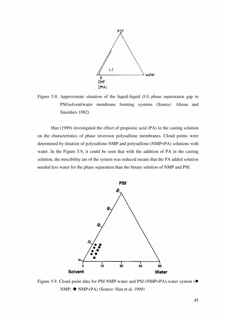
45

Figure 5.8. Approximate situation of the liquid-liquid (l-l) phase separataion gap in

PSf/solvent/water membrane forming systems (Source: Altena and

Smolders 1982)

Han (1999) investigated the effect of propionic acid (PA) in the casting solution

on the characteristics of phase inversion polysulfone membranes. Cloud points were

determined by titration of polysulfone-NMP and polysulfone-(NMP+PA) solutions with

water. In the Figure 5.9, it could be seen that with the addition of PA in the casting

solution, the miscibility are of the system was reduced means that the PA added solution

needed less water for the phase separation than the binary solution of NMP and PSf.

Figure 5.9. Cloud point data for PSf-NMP-water and PSf-(NMP+PA)-water system (�

NMP; � NMP+PA) (Source: Han et al. 1999)

46


PMMA/Solvent/Nonsolvent Systems

In the study of Lai et al. (1998), the ternary phase diagrams of PMMA/n-butyl-

acetate/n-hexane, PMMA/acetone/water and PMMA/acetone/n-hexane were constructed

by theoretical calculation and experimental measurement. Experimental cloud points

were measured by titrating the PMMA solutions with water until the onset of turbidity

and binodal curves were calculated by using Flory Huggins theory for three-component

systems.

Figure 5.10. Comparison between the calculated and experimental binodal curves for

PMMA/acetone/water system at 25°C (Source: Lai et al. 1998)

Good agreement was obtained between the calculation and the measurement by

using concentration-dependent water/acetone and acetone/PMMA interaction

parameters and constant water/PMMA interaction parameters as shown in Figure 5.10.

χ13 (water-PMMA interaction parameter) was determined as 2.34 by using swelling-

equilibrium measurements. g23 (acetone-PMMA interaction parameter) at different

concentrations was measured as g23 = 0.48 + 0.23ν3 by Cahn microbalance. The

concentration of polymer solution was determined by measuring the amount of solvent

absorbed by PMMA. g12 (water-acetone interaction parameter) was calculated by using

the data of excess Gibbs free energy or activity coefficients obtained from literature

sources and found as g12 = 0.661 + 0.417 / (1-0.755u2).

47

CHAPTER 6

MODELING OF SORPTION PROCESS

The transport behavior of small molecules in polymers strongly depends on the

polymer structure and mobility. Diffusion in polymers is one of the fundamental

problems associated with a variety of industrial applications including controlled drug

release systems, packaging and separation technologies.

“When a penetrant diffuses into a polymer film, the macromolecules rearrange

toward a new configuration with a relaxation rate that depends on temperature as well as

on solvent concentration”. The nature of the transport process is determined by the

relative timescales of the diffusion and relaxation processes (Rodriguez 2003).

In the next sections, typical sorption kinetics and model equations to describe

these kinetics are given. These models are combined with experimentally measured

sorption curves to determine diffusion coefficients and relaxation times. The diffusion

regimes and features of diffusion in glassy polymers are also discussed.

6.1. Typical Sorption Kinetics

Results of the typical sorption experiments are generally presented by plots of

mass uptake as a function of square root of time (t1/2). The response of the polymers in

the presence of a penetrant can be categorized into different classes based on the rates of

penetrant diffusion and relaxation of the polymer. Sorption kinetics as categorized

according to the shape of the mass uptake (Mt/M∞) as a function of t as shown in

Figure 6.1.

6.1.1. Case I Sorption (Fickian Sorption)

This type of diffusion occurs when the rate of diffusion is significantly slower

than the rate of relaxation of the polymer chains (Ghi et al. 2000). When the fractional

mass uptake is plotted as a function of square root of time, the Fickian sorption curves

exhibit the following behavior:

48

Figure 6.1. Typical sorption kinetics: (a) Fickian; (b) Two-stage; (c) Sigmoidal; (d)

Case II (Source: McDonough 2004)

1. In the initial stages of the sorption process, the sorption curve becomes linear.

2. This linear region extends up to 60% of the uptake (Mt/M∞ = 0.6).

3. Above the linear portion, the sorption curve becomes concave with respect to the

t1/2 axis.

4. The sorption curves obtained for different values of the film thicknesses when

plotted as Mt / M∞ versus t1/2 / L coincide with each other.

5. The sorption and desorption curves at the same temperatures coincide with each

other.

Penetrant diffusion through rubbery polymers is generally Fickian. The

polymers in the rubbery state respond rapidly to changes in their condition. If they are

above their glass transition temperature, the polymer chain adjust so quickly in the

presence of penetrant that they do not show diffusion anomalies (Crank 1975). This

49

sorption behavior is also observed in glassy polymers at low penetrant activities (Dhoot

2004).

If Fickian diffusion controls the penetrant uptake in a polymer film of uniform

thickness, then the time required to reach equilibrium is determined by the diffusivity of

penetrant in the polymer film (Crank, 1975):

(6.1)

In order to determine diffusivity of penetrant in the polymer film for Case I

sorption, unsteady-state process is modeled using following assumptions:

1. The diffusion process is one dimensional transport process in a polymer film of

thickness L

2. Diffusion process is a viscous Fickian process

3. There is no chemical reaction between the penetrant and the polymer film.

4. The diffusion process is isothermal

5. The vapor phase is essentially pure

6. The mutual diffusion coefficient D is independent of concentration during each step

of the sorption process

Under these assumptions, sorption process is described by the following

equation

(6.2)

Initially, the concentration of the penetrant, C0, in the polymer is same

everywhere;

(6.3)

At times t > 0, the concentration of the penetrant at the surface is constant and

equal to its equilibrium concentration, Ceq

00 CCt =→=

2

2

xC

DtC

∂∂=

∂∂

DL

teq

2

≈

50

t > 0 → x = L C = Ceq (6.4)

and concentration gradient at the lower surface is zero since this surface is impermeable

to penetrant vapor

t > 0, x = 0, 0=∂∂ xC (6.5)

Analytical solution of equation (6.2) through equation (6.5) is given by Crank

(1975) as:

(6.6)

Equation (6.6) is integrated from x = 0 to x = + L, then the dimensionless uptake

is obtained as follows;

(6.7)

where Mt and M∞ are the penetrant mass uptake at time t and at equilibrium,

respectively; while M0 is the mass of the polymer film at the beginning of each sorption

step; D is the diffusion coefficient; and L is the film thickness (Crank 1975). Diffusivity

can be estimated by minimizing the difference between experimental fractional mass

uptake data and theoretical ones calculated from Equation 6.7.

Crank (1975) has shown that at short times, t → 0, Equation (6.7) can be

simplified as follows;

(6.8)

Equation (6.8) indicates that at short times, uptake curve becomes linear and

diffusion coefficient can be easily calculated from the slope of the plot of ∞′′ MM t /

versus t1/2.

{ } ∞

=

++−+

−−=−−

on

n

Lxn

LtnDnCC

CC πππ

)12(cos/)12(exp

12)1(4

1 222

01

0

{ }222

022

0

0 /)12(exp)12(

181 LtmD

mMMMM

MM

m

tt ππ

+−+

−=−−

=′′

∞

=∞∞

2/1

2

2��

�

�=′′

∞ LDt

tMM t

51

6.1.2. Case II Sorption

Case II sorption is considered as a typical non-Fickian behavior (Figure 6.1d).

This type of diffusion occurs when the rate of penetrant diffusion is greater than the rate

of relaxation of the polymer chains (Ghi et al. 2000), and is strongly depend on swelling

kinetics (Chin et al. 1999). The main feature of Case II sorption is a sharp diffusion

front separating a swollen penetrated distance from a glassy core. In addition, the

penetrant weight uptake is proportional to time rather than the square root of time, as in

other cases (McDonough 2004).

Hopfenberg and Frisch (1969) rewrote the Fick’s second law (Equation 6.2),

incorporating a term to describe the constant velocity movement of a penetrant front.

(6.9)

According to Hopfenberg and Frisch, anomalous penetrant uptake could be

expressed by the motion of the solvent front described by a linear combination of the

two effects:

(6.10)

where ν is the front velocity, Na and Nb are the mole fraction of each component and ka,

kb are uptake rate constants for pure liquid a or b.

Thomas and Windle observed that methanol absorption in PMMA obeys Case II

sorption. They assumed that diffusion of the solvent in a swollen element is much faster

than in a glassy element. When solvent molecules enter the element, they clear the way

for following molecules; the plasticizing effect causes next molecules to enter more

rapidly. Accumulation is initially faster than transport to the next element and this result

in a sharp front (van der Wel and Adan 1999).

6.1.3. Case III Sorption

Case III sorption or anomalous diffusion occurs in the transition region between

Case I and Case II sorption, when the rates of polymer relaxation and penetrant

��

�

� −∂∂

∂∂=

∂∂

CxC

Dxt

C ν

tkNtkN bbaa += 2/1ν

52

diffusion are comparable. There are two types of anomalous diffusion, two-stage

sorption and sigmodial sorption.

6.1.3.1. Two-Stage Sorption

Two-stage sorption is generally defined as anomalous type of absorption. It is

named ′two-stage’ sorption because the sorption curve appears to be composed from

two different parts: (1) fast Fickian sorption; (2) slow non-Fickian. The sorption curve is

Fickian from the start until it starts to level off. Instead off reaching the equilibrium

level which is typical for Fickian sorption, the curve is extended through a non-Fickian

part. Finally equilibrium is reached for all instances (van der Wel and Adan 1999).

General appearance of two-stage sorption is shown in Figure 6.1b. This type of

diffusion behavior is often observed for organic vapor sorption in glassy polymers such

as benzene in PET, acetone in PET, ethyl benzene in polystyrene (Dhoot et al. 2001).

A theory, describing the features of ‘two-stage’ sorption, has been proposed by

Berens and Hopfenberg in 1978 (Berens and Hopfenberg 1978). According to their

diffusion-relaxation model, sorption process is composed of two phenomenologically

independent contributions: a diffusion part MF(t) governed by Fick’s laws and a

structural part MR(t), resulting from polymer relaxations. The total weight gain at time t

is then expressed as the linear superposition of these contributions:

(6.11)

It is generally assumed that viscoelastic processes in polymers are described by a

distribution of relaxation times, so MR(t) is given by:

(6.12)

where M∞,i represents the equilibrium sorption due to the ith relaxation process, and ki

is the first-order relaxation constant of the ith relaxation process. In the study of Berens

and Hopfenberg (1978), this model has been developed for diffusion in spherical

particles, but it has also been applied to diffusion in polymer films (van der Waal and

Adan 1999).

)()()( tMtMtM RF +=

[ ] −−= ∞ )exp(1)( , tkMtM iiR

53

Two-stage sorption, a non-Fickian phenomenon, has been observed by several

researchers. A two-stage model incorporates Fickian diffusion at short times and

protracted structural relaxation at long times (Dhoot et al. 2001). The diffusion process

controls mass uptake at short times and polymer relaxation controls mass uptake at long

times. The intermediate plateau region observed in each plot separates the diffusion-

controlled and relaxation-controlled regimes of mass transfer. This sorption kinetics is

often described using the following empirical model:

(6.13)

where D is the average diffusion coefficient, αR is the fraction of weight uptake

controlled by polymer relaxation, τR is the time constant characterizing the long time

drift in mass uptake toward equilibrium, tD is a delay factor associated with a delay in

the beginning of structural relaxation. αR must lie between zero and one and can be

determined from the intermediate plateaus which are representative of the fraction of

mass uptake controlled by structural relaxation. Typical values of tD range from 0 to

Dl /2 , which corresponds to the end of Fickian diffusion.

At short times, the fractional mass uptake, ∞MM t / increases linearly with the

square root of time, which is characteristic of sorption kinetics controlled by Fickian

diffusion and can be modeled as given in Equation 6.8. The average Fickian diffusion

coefficient can be estimated from a best fit of data to the analytical model.

(6.14)

At longer times, the mass uptake shows a protracted, non-Fickian asymptotic

approach toward equilibrium. Protracted stage of uptake is associated with mass uptake

controlled by the viscoelastic relaxation of the polymer chains to accommodate

penetrant and can be modeled as

( )

��

��

��

��

� −−−+

��

��

��

��

� +−×+

−−= ∞

=∞

R

DR

nR

t

tt

ltnD

nMM

τα

ππ

α

)(exp1

)12(exp

)12(18

110

2

22

22

∞

=∞��

�

� +−×+

−=− 0

2

22

22 4)12(

exp)12(

181

)1( nR

t

ltnD

nMM π

πα

54

(6.15)

In the study of Dhoot et al. (2001), αR was obtained from the plateaus, in the

sorption curves while D was calculated from the slope of the initial kinetic data, which

is linear in t1/2, using the following relation:

(6.16)

The parameters τR and tD were obtained by fitting the long-time kinetic data to

the following equation:

(6.17)

Equation (6.14) clearly shows that when αR = 0, then Equation (6.7) is recovered

which is used to analyze Fickian sorption curves.

6.1.3.2. Sigmoidal Sorption

Sigmoidal sorption curves are S-shaped, showing a point of inflection (Figure

6.1c). The transport process in the film is Fickian, but due to the slow establishment of

equilibrium at the surface of the film, kinetics show anomalous behavior.

Long and Richman proposed a variable surface-concentration model to describe

an anomalous, sigmoidal sorption curve. Rodriguez et al. (2003) used a simplified

version model, suggested by Crank (1975). It is assumed that the diffusion process is

Fickian, and that the surface concentration approaches exponentially the equilibrium

concentration, C0, at the selected activity:

(6.18)

��

��

� −−−=∞ R

DR

t ttMM

τα )(

exp1

��

�

�=

−∞

24)1(

/l

DtMM

R

t

πα

RR

DR

t ttt

MM

τα −��

�

�

�+=��

�

�

�−

∞

ln1ln

[ ])exp(1),( 0 tCtLC β−−=

55

where β is the inverse of the characteristic time for attaining saturation at the surface. If

β → ∞, the surface concentration rises instantaneously to C0 and the curve has the

characteristic initial linear portion followed by the approach to the equilibrium as seen

in Fickian sorption process. The solution of Fick’s second law with the boundary

conditions given by Equation 6.19 and with a constant diffusion coefficient D is:

(6.19)

Figure 6.2 shows the influence of the value of β on the shape of the sorption

curves.

0 20 40 60 80 100 120 140 160 1800.0

0.2

0.4

0.6

0.8

1.0

1.2

= 0.0001 = 0.01 = 0.1 = 1000

βββ

∞′′

MM t

)( 5.0timet

β

Figure 6.2. Calculation of sorption curves for different β values

∞

=∞

��

��

��

��

�+−+

��

��

� +−−

��

�

�

��

�

�

��

�

��

�

�−−=

′′

0

2

222

222

2

2/122/1

2

4)12(1)12(

4)12(exp

8tan)exp(1

n

t

lD

nn

lt

nD

Dl

lD

tMM

βπ

π

πβ

ββ

56

6.1.4. Sorption Overshoot

In some cases, a plot of the fractional penetrant uptake Mt / M∞ versus t0.5

presents a characteristic maximum before attainment of the final equilibrium value. This

feature of uptake kinetics is called ‘sorption overshoot’, and it is in general due to a

rearrangement of the polymer chains following plasticization induced by a penetrant. In

the literature, four possible reasons are reported for overshooting of the equilibrium

penetrant concentration. First, sorption overshoots are observed during sorption of

strongly interacting liquids or vapors in initially amorphous, crystallizable glassy

polymers. The newly formed crystalline regions are impenetrable and part of the sorbed

penetrant is expelled out thus producing the maximum in the sorption curve.

Second, a penetrant-induced melting of unstable crystals and subsequent

formation of stable crystals may lead to a sorption maximum without a net change in the

crystallinity fraction. Thermally induced structural reorganizations, such as primary and

secondary crystallization and melting were verified by modulated differential scanning

calorimetry (MDSC) in the study of Alentiev et al. (2001).

Third, sorption overshoot in rubbery and glassy polymers may occur from a

slow relaxation of the polymer chains to a more compact structure. Although most of

these types of effects are usually mentioned in glassy polymers, overshoots in rubbery

polymers are also reported in literature (Ghi et al. 2000). In glassy polymers, the

overshoot is related to the relaxation processes of the polymer chains as mentioned in

Etxeberria et al. (2000). The velocity of the solvent diffusion in the polymer is faster

than the chain movements at high activities. This fast sorption stresses the polymeric

chains facilitating relaxation processes and accompanied by plasticization effect of the

sorbed solvent. These structural rearrangements cause a decrease in the solvent

solubility and existence of overshoots in the sorption kinetics. At lower activities, the

solvent absorption is not very fast so the effect is expected smaller. When a slow

process such as swelling partially controls the sorption kinetics, thickness of the sample

becomes an important parameter (Hoyt and Balik 1996).

Finally, release of domestic components of the polymer matrix after contact with

liquid may cause a maximum in kinetic sorption (Rodriguez et al. 2003).

57

6.2. Diffusion Regimes

When a penetrant diffuses into a polymer film, the macromolecules rearrange

toward a new configuration with a relaxation rate. The relative time scales of the

diffusion and relaxation processes determine the nature of the transport process

(Rodriguez 2003). Vrentas defined a diffusive Deborah number, De, as the ratio of two

characteristic times, relaxation time for the polymer-solvent systems (λm) and the

characteristic diffusion time (θD) (Vrentas and Duda, 1979).

(6.20)

where θD is defined as DL /2 . When De << 1, diffusion rate is significantly slower than

the relaxation rate of the polymer chain, and viscous Fickian diffusion is observed. In

this case, conformational changes in the polymer take place essentially instantaneously

and both solvent and polymer behave like purely viscous fluids (Vrentas and Duda

1979). When the Deborah number is sufficiently large, the diffusive process is fast

compared to the molecular relaxation, and this type of diffusional transport can be

denoted as elastic Fickian diffusion. There is essentially no time variation of the

structure of the polymer during diffusion process. Under these conditions, a solvent

molecule moves in a material which appears to have the properties of an elastic solid

(Vrentas and Duda 1979). If the Deborah number is of the order of unity, the molecular

relaxation and diffusive transport processes occur in comparable time scales, and

rearrangement of polymer chains and movement of solvent molecules take place

simultaneously. This type of diffusion transport is known as viscoelastic (anomalous)

nonFickian diffusion (Vrentas 1977). Fickian behavior is expected for rubbery polymers

at temperatures above the glass transition temperature, whereas anomalous sorption is

more likely to occur for polymer-penetrant mixtures in the glassy state (Rodriguez

2003). The sorption curves ( ∞′′ MM t / versus Lt /2/1 ) for films of different thicknesses

give a single curve for the cases of viscous Fickian and elastic Fickian diffusion means

that the binary diffusion coefficient of the polymer-solvent systems is independent of L.

However, in the case of anomalous, non-Fickian diffusion, the sorption curve for films

of different thicknesses may not yield a single curve, i.e., the mutual diffusion

coefficient may depend on L. Anomalous features may depend on time-dependent

DmDDEB θλ /)( =

58

surface concentration and anisotropic dimensional changes in the polymer sample other

than polymer relaxation (Rodriguez 2003).

6.3. Diffusion in Glassy Polymers

In glassy polymers, deviations from Fickian behavior are generally observed.

These deviations are considered to arise as a consequence of the finite rate of polymer

structure reorganization in response to the sorption or desorption of penetrant

molecules. Anomalous effects may be related to the influence of the changing polmer

structure on solubility and diffusional mobility, or they may arise from the internal

stresses exerted by one part of the medium on another as diffusion proceeds (Crank

1975). When penetrant sorption is realized by swelling of the polymer, any time

dependent resistance to changes in the volume of the polymer can lead to non-Fickian

sorption kinetics. Non-Fickian diffusion is commonly observed in sorption of organic

vapors into glassy polymers. When the penetrant swells the polymer, local stresses

occur and these stresses can be quite high to cause mechanical failure in the polymer

(Dhoot 2004). If the polymer chains do not deform significantly upon penetrant sorption

or the chains reorganize relative to the penetrant diffusion, Fickian behavior is observed.

59

CHAPTER 7

EXPERIMENTAL

7.1. Materials

Polysulfone (CAS: 25135-51-7, Mw: 56,000 g/mol) and PMMA (CAS: 9011-14-

7, Mw: 15,000 g/mol) used in this study were obtained from Aldrich. The physical

properties of the polymers are provided in Table 7.1. For polysulfone; ultapure water

and ethanol (Panreac, ρ: 0.793 g/cm3) are used as nonsolvents, THF (Panreac, ρ: 0.636

g/cm3), NMP (1-methyl-2-pyrrolidinone, Aldrich, ρ: 1.033 g/cm3) and chloroform

(Riedel, ρ: 1.47 g/cm3) are used as solvents. For PMMA; ultrapure water and

formamide (Aldrich, ρ: 1.134 g/cm3) are used as nonsolvents, while acetone (Merck, ρ:

0.79 g/cm3) and THF are used as solvents. All chemicals were used as received without

further purification.

Table 7.1. Properties of polymers

Properties Polysulfone PMMA

Mn (g/mol) 26,000 14,286

Mw (g/mol) 56,000 15,000 by GPC

Density (g/mL) 1.24 1.17

Tg (°C) 190 82

Supplier Aldrich Aldrich

CAS No 25135-51-7 9011-14-7

7.2. Film Preparation Method

Preparation of a polymer film strongly influences the structure of the film

formed, which plays an important role on the diffusion behavior. In glassy polymers, the

film preparation method is very important and all films for the same polymer are

prepared following the same procedure to standardize their histories.

60

7.2.1. Polysulfone Film Preparation

Firstly polysulfone was dissolved in NMP and left on a magnetic stirrer for 1

day to get a clear solution. Polymer solutions were prepared at 20 wt% concentration

when 10 and 30 µm films were aimed to obtain. These films were prepared by casting

the solution on a clean and smooth glass substrate by knives with exactly dimensioned

slits of 120 and 300 µm, through an automatic film applicator (Sheen 1133N). When

films of 1-3 µm were prepared, the polymer solutions were prepared at 5 and 10 wt%.

These thin films were prepared when long terms were required to attain the equilibrium,

in order to shorten the required time. The cast films were put into an oven under

vacuum. The temperature of the oven was raised to 190.5°C (4.8°C/min), above the

glass transition temperature of the polymer and kept in the oven for 3 day. The films

were dried in a vacuum oven at 100 mb to remove the solvent completely. To obtain

annealed films of reproducible quality, the oven was switched off after 3 days and films

were cooled slowly (1.2°C/min) for one day. After removing from the oven, the films

were easily detached from the glass surface with a small amount of water. The film

preparation was schematically shown in Figure 6.1. The dry-film thicknesses were

measured using a micrometer (Testo) at different locations. The accuracy of the

micrometer was ±0.03 mm. And the film thicknesses were measured accurately with

Scanning Electron Microscope (SEM) to check the results. The thicknesses of the

samples were measured from several different points and the average were used for

subsequent calculation. The prepared films were kept in desiccator. Differential

scanning calorimetry and thermal gravimetric analysis were used to ensure full removal

of the solvent.

Figure 7.1. Schematic representation of film preparation procedure

POLYMER

Dissolution Casting

Drying ( >Tg ) &

Annealing

SOLVENT

61

Pieces in the size of approximately 11 × 11 mm were cut from the raw films. The latter

size was used to fit the film onto the trays of the small stainless steel sample holder.

7.3. Characterization Studies

7.3.1. Scanning Electron Microscope (SEM) Analysis

Scanning Electron Microscope (Philips, XL-30SF6) was used to investigate the

morphology of the films prepared and to measure the average thicknesses of the films.

In the preparation stage, the film samples were coated with a thin gold layer to enable

the transport of electrons from the electron beam that were not reflected or transformed

to secondary electrons. The samples were placed in a sample holder and evacuated.

Then the SEM pictures were obtained at certain magnifications to see the details of the

films.

7.3.2. Differential Scanning Calorimetry (DSC) Analysis

Differential Scanning Calorimetry (Shimadzu DSC 50) was used to be ensure

the full removal of the solvent from the polysulfone films. The boiling point of NMP

used in film preparation is 220°C, as a result the ensurement was achieved by DSC

analysis. 3.1 mg polysulfone film sample was placed in an aluminum pan and heated at

a constant rate from 20°C to 500°C with a heating rate of 1°C/min until 30°C and

5°C/min above 30°C using nitrogen as a purge gas with a flow rate of 40 mL/min.

7.3.2. Thermal Gravimetric Analysis (TGA)

Thermal gravimetric analysis (TGA) was performed to prove no residual is left

in the polysulfone films. Analysis was performed with Shimadzu TGA51 under nitrogen

flow at a rate of 30 mL/min. 11.07 mg polysulfone film was placed in an aluminum pan

and heasted continuously from 20°C to 600°C at a rate of 10°C/min.

62

7.4. Determination of Cloud Point Curves

The cloud point curves were determined by the titration of homogeneous

polymer solutions with nonsolvents until the onset of turbidity. The concentration of

polymer solutions was varied between 8-22 w %. Quantities of polymer was determined

by using an electronic balance capable of reading up to ±0.0001 g and put into HPLC

vials (10 mL) with its solvents. The flasks were capped tightly with a rubber septum

stopper to avoid evaporation, and left in a fast-acting thermostat bath for one day in

order to obtain homogeneous solutions (Figure 7.2). Afterwards, nonsolvents were

added to the clear polymer solutions by a microsyringe (Agilent) with an accuracy of

±0.001 mL, through the septum until turbidity was observed. During titration, the

solutions were well stirred and kept at a constant temperature by a fast-acting thermostat

bath. The composition at which permanent turbidity first occurred is called the cloud

point, which represents the composition where the phase transition occurred and was

determined by measuring the amount of nonsolvent added.

Figure 7.2. Fast-acting thermostated bath

7.5. Magnetic Suspension Balance Analysis

7.5.1. Experimental Set-up and Operating Procedure

Magnetic suspension balance used for sorption measurements consists of four

groups as main sorption unit, control unit, computer and supporting units (constant

temperature baths, cold trap, heating tape, temperature controller, pressure transducer,

tubings, fittings and ball valves) as shown in Figure 7.3.

63

Figure 7.3. Digital photograph of experimental set-up in laboratory. 1, balance; 2,

sorption cell; 3, circulating water bath; 4, water bath; 5, pressure

transducer; 6, vacuum pump; 7, cold trap; 8, heating tape; 9, temperature

controller; 10, control unit; 11, computer

The resolution of the balance is 1 µg, the maximum load is 5 g, and the

reproducibility of the measurements is ±2 µg. The magnetic suspension balance can

withstand to high pressures up to 150 bars and temperatures up to 250°C. Housing of

copper chrome zirconium is used to separate the measuring room between the

suspension magnet and the electromagnet and its the inner surface is gold plated. The

lower part of the housing is made of stainless steel. The sealing between the measuring

cell and the weighing instrument is metal seal coated with gold. In order to protect the

permanent magnet, it is completely sealed in a stainless steel housing. The entire

interior volume of the magnetic suspension balance is thermostated to the sample

temperature by means of double walled thermostated jacket which completely surrounds

the measuring cell (Figure 7.4).

6

7

4

9

5

1

2

10

3

11

64

Figure 7.4. Double walled jacket for thermostating measuring cell with a circulating

fluid (Source: WEB_2 2007)

A water bath (Polyscience, 3) with an accuracy of ±0.5°C and the operating

range between 5°C above the room temperature and 100°C is used to circulate the fluid

through the jacket. A thermocouple probe inserted into the column just below the

sample holder, measures the temperature of the fluid in the column. The polymer films

are put into a stainless steel sample holder and it is suspended from a permanent

magnet. Sample holder consists of 5 stacked trays and each tray has 11.96 × 12.46 mm

dimensions. Solvent vapor is prepared in a solvent flask inserted into a constant

temperature bath (Heto, 4) which works between room temperature and 100°C

(accuracy ±0.5°C). The vapor pressure of the solvent is measured by a pressure

transducer (Omega, 5) operating within a range of vacuum up to 1 atm with an accuracy

of 0.25% full scale. Vacuum is applied to the column by using a rotary vane pump

(Vacuubrand, 6) which can provide vacuum up to 10-4 mbar. A cold trap (7) made of

pyrex is placed between the sorption column and the vacuum pump. All tubings and

fittings (Swagelok) are made of stainless steel and valves (Swagelok) exposed to solvent

vapor are made of teflon. Heating tape (8) is wrapped on all solvent vapor line to

prevent condensation of solvent vapor. The temperature of the heating tape is controlled

by a temperature controller (Love controls, 9) with an accuracy of ±0.5°C.

The magnetic suspension and weight measurements can be controlled with the

MessPro software and can be operated from the control unit shown in Figure 7.5. The

suspension control unit consists of a main power switch, a dial to control the suspension

coupling, and another dial on the rear of the unit to check the voltages in the system.

The dial on the front of the unit can be set to OFF, zero point (ZP) and measuring point

(MP) positions. In zero point position, the polymer sample is set down on a support

such that the balance only measures the weight of the suspension coupling. In MP, the

balance lifts the basket containing the polymer sample.

65

Figure 7.5. Illustration of suspension control and balance indicator units


At the beginning of a typical experiment, five pieces in the size of approximately

11 × 11 mm are cut from the raw films. The sheets of the films are laid onto the trays of

the sample holder and heated (4.8°C/min) to above the glass transition temperature of

the polymer under 100 mb vacuum in a vacuum oven (Memmert) for a second time.

After 2 hours at those conditions, the oven is cooled down at a rate of (1.2°C/min) for

another 2 hours. The cooling process allows the film attach itself to the surface of the

tray. Thus, the sorption experiment is carried as a diffusion from one side into the film.

After that, sample holder is placed into the column, then the stainless steel jacket is

located around the column and connected to water bath. The tubings and the fittings are

heated up to 60°C by using heating tape and evacuated by a vacuum pump in order to

remove water vapor condensated inside of the tubings. Then the program in the software

is started and the temperature of the water bath is set 1°C above the desired temperature

of the column. The system is allowed to reach equilibrium in 24 hours. After 24 hours,

the column is evacuated for one hour via two connections to a vacuum pump. Then

solvent line is evacuated for half an hour. When vapor-liquid equilibrium is achieved in

the solvent flask at the desired temperature of the solvent, the pressure of the solvent

vapor is measured by the pressure transducer and checked with the literature values.

Meanwhile, the program in the software is started and measurement is taken for about

every 5 seconds. After stable reading is observed, the solvent vapor is sent into the

column by opening the valve. The weight change of the sample is followed as a function

of time as shown in Figure 6.6. The software allows storing and drawing of all data

measured.

66

Figure 7.6. Typical computer software output obtained from sorption experiment

Once the polymer reaches an equilibrium state at a specific penetrant vapor

pressure level, the valve is closed and an increase in the vapor pressure of the solvent is

induced by increasing the temperature of the constant temperature bath. The step change

in the column is produced by opening the valve and letting the solvent vapor at a new

vapor pressure level into the column. This procedure is repeated until the temperature

of the solvent vapor in the flask reaches to 5°C below the temperature of the column to

avoid condensation in the column. A computer records all temperature and the weight

change of the sample as a function of time automatically. The number of runs in a given

series for each temperature of the column depends on the amount of the penetrant

absorbed. Usually step size is adjusted to make difference between the equilibrium and

initial mass of the penetrant, small. This adjustment allows assuming constant

diffusivity within this range and negligible swelling of the polymer film. Schematic

representation of the experimental system is shown in Figure 7.7.

67

Figure 7.7. Schematic representation of the experimental system. 1, circulating liquid

thermostat; 2, balance; 3, magnetic suspension coupling; 4, sorption cell; 5,

pressure transducer; 6, water bath including solvent flask; 7, cold trap; 8,

vacuum pump

7.5.2. Forces Affecting the System

Buoyancy of the solvent vapor in the measuring cell affects the measurement,

thus, the buoyancy of the substrate at different vapor pressures and densities should be

taken into account. Figure 7.8 shows all forces affecting the system. A balance of forces

for the whole system in the vertical direction gives an equation for the determination of

the amount of solvent vapor absorbed by the polymer.

1

2

4

5

6

7

8

3

68

Figure 7.8. Forces affecting on the system

(Source: Rubotherm)

These forces are:

Measurement force or signal detected by the balance

(7.1)

The force resulting from the absorption of an amount of vapor by the sample

(7.2)

AF1

MF

GF

AF2

gmAF absorbed ⋅=1

gSMF MP ⋅=

69

Gravitational force affecting the system in the vacuum

(7.3)

Ascending force affecting the system

(7.4)

If the balance of forces in vertical direction is written as

(7.5)

then, the absorbed amount of vapor can be determined from Equation 7.6.

(7.6)

7.5.3. Determination of Volumes

In order to determine the ascending correction of the collected measuring data,

the volume of the whole device should be determined. The explanation of the system is

given in Figure 7.9. The total volume of the system as defined as follows:

(7.7)

To determine these volumes, first of all, the weights of cage, hook and sample

cage are measured:

Wcage+hook = 1.8260 g

Wsample cage = 2.5852 g

Wsuspension magnet = 3.2577 g

21 AFMFGFAF +=+

[ ] gVVVAF samplecagevaporsamplehookcagevapor ⋅++⋅= ++ρ2

gmGF vac ⋅=

[ ] vacsamplecagevaporsamplehookcagevaporMPabsorp mVVVSm −++⋅+= ++ρ

samplecagehookcagesystem VVVV ++=

70

Figure 7.9. Explanation of the system

(Source: Rubotherm)

Then, these weights are corrected for bouyancy using the following equation:

(7.8)

In this equation; M is the buoyancy corrected weight, W is the weight displayed

by the balance, ρA is the density of air (1.2 kg/m3), and ρMG is the density of the material

used in the balance (Stainless steel, 8000 kg/m3).

According to this equation, buoyancy corrected weights are calculated as

follows:

Bouyancy corrected weight of cage and hook:

��

�

�

��

�

�

−=

MG

A

WM

ρρ

1

1

71

M = 1.8262 g

Bouyancy corrected weight of sample cage:

M = 2.5856 g

Mass of cage, hook and sample cage:

4118.45856.28262.1 =+ g

Then, volume of cage, hook and sample cage:

Vcage+hook+sample cage = ( ) 5514.088262.15856.2 =+ cm3

72

CHAPTER 8

RESULTS AND DISCUSSIONS

8.1. Characterization of the Polymer Films

8.1.1. Determination of the Morphology and Thickness of the Polymer

Films by Using Scanning Electron Microscope

Figure 8.1 shows the SEM picture of cross section of the polysulfone film.

Nonporous, homogeneous film structure was observed. Using SEM pictures, thickness

of each film was determined from an average of 3 or 6 measurements.

Figure 8.1. SEM picture of the cross section of polysulfone film used to measure film

thickness

73

8.1.2. Differential Scanning Calorimetry (DSC) Analysis of the

Polysulfone Films

Figure 8.2 shows the DSC curve of the polysulfone film. In DSC, energy is

given to both sample and a reference material and the difference between the sample

and the reference is used as a measure of thermal events. Around 190°C, a decrease in

the slope of the heat flow curve was observed which corresponds to change from glassy

to rubbery state. From this decrease, the glass transition temperature of the polysulfone

was determined as 189°C. Amount of heat given to the sample compared to the

reference increases significantly above 530°C and a negative peak was observed due to

the degradation of the polymer.

Temperature (oC)

0 100 200 300 400 500 600

Hea

t Flo

w (m

W)

-2.5

-2.0

-1.5

-1.0

-0.5

0.0

0.5

Figure 8.2. Differential Scanning Calorimetry analysis of polysulfone film

8.1.3. Thermal Gravimetric Analysis (TGA) of the Polysulfone Films

Figure 8.3 shows TGA curve of the polysulfone film. According to this figure,

weight loss of the sample was observed above 281.3°C. Until 220°C (boiling point of

NMP), 0.03 mg weight loss was observed which indicated that there is no significant

74

amount of residual NMP in the film. At 599.9°C, only 50.5% of the total weight was

lost.

Temperature (oC)

0 100 200 300 400 500 600

TGA

(mg)

5

6

7

8

9

10

11

12

Figure 8.3. Thermal Gravimetric Analysis of polysulfone film

8.2. Determination of Cloud Points Experimentally

Figures 8.4 through 8.9 illustrate the experimental cloud points of the systems

PSf/NMP/water, PSf/THF/water, PSf/NMP/ethanol, PSf/THF/ethanol,

PMMA/acetone/water, PMMA/THF/water, PMMA/acetone/formamide,

PMMA/THF/formamide at 40°C, which show the miscible region of polymer and

solvent with nonsolvent.

8.2.1. Comparison of Experimental Cloud Points with Previous Studies

Kim et al. (1997) determined the experimental cloud points for PSf/NMP/water

and PSf/THF/water systems at 15°C and 60°C by a titration method and their cloud

points measured at 15°C were compared with those determined in this study. Figures

8.4 and 8.5 show that cloud point curves obtained in this study for PSf/THF/water and

PSf/NMP/water are in good agreement with those reported by Kim et al. (1997). These

results proved the accuracy of the experimental procedure used in this study. Kim et al.

have observed that the effect of temperature on the cloud point curve is very small.

75

Hence, the comparison of their data collected at 15°C is reasonable with those collected

in this study at 25°C.

Water0.0 0.1 0.2 0.3 0.4 0.5 0.6 0.7 0.8 0.9 1.0

PSf

0.0

0.1

0.2

0.3

0.4

0.5

0.6

0.7

0.8

0.9

1.0

THF

0.0

0.1

0.2

0.3

0.4

0.5

0.6

0.7

0.8

0.9

1.0

This study (25oC)Kim et al., 1997 (15oC)

Figure 8.4. Comparison of experimental cloud point curves for PSf/THF/Water system

Water0.0 0.1 0.2 0.3 0.4 0.5 0.6 0.7 0.8 0.9 1.0

PSf

0.0

0.1

0.2

0.3

0.4

0.5

0.6

0.7

0.8

0.9

1.0

NMP

0.0

0.1

0.2

0.3

0.4

0.5

0.6

0.7

0.8

0.9

1.0

This study (25oC)Karimi et al., 2005 (25oC)

Figure 8.5. Comparison of experimental cloud point curves for PSf/NMP/Water system

76

8.2.2. Effect of Solvent Type on Ternary Phase Diagram

The cloud points given in Figure 8.6, show that the region of the homogeneous

phase is slightly larger in the PSf/NMP/water system than in the PSf/THF/Water system

at the same temperature. The influence of solvent type on the cloud points become more

pronounced when ethanol is used as a nonsolvent. It was observed that homogeneous

phase region is larger in the PSf/NMP/ethanol than in the PSf/THF/ethanol system at

40°C as shown in Figure 8.7.

In the case of PMMA, the homogeneous phase region is not influenced by

solvent type which are acetone and THF when both water and formamide are used as

nonsolvents as shown in Figures 8.8 and 8.9.

Water0.0 0.1 0.2 0.3 0.4 0.5 0.6 0.7 0.8 0.9 1.0

PSf

0.0

0.1

0.2

0.3

0.4

0.5

0.6

0.7

0.8

0.9

1.0

Solvent

0.0

0.1

0.2

0.3

0.4

0.5

0.6

0.7

0.8

0.9

1.0

PSf/NMP/Water (25oC)PSf/THF/Water (25oC)

Figure 8.6. Experimental cloud points for Polysulfone/Solvent/Water system

77

Ethanol0.0 0.1 0.2 0.3 0.4 0.5 0.6 0.7 0.8 0.9 1.0

PSf

0.0

0.1

0.2

0.3

0.4

0.5

0.6

0.7

0.8

0.9

1.0

Solvent

0.0

0.1

0.2

0.3

0.4

0.5

0.6

0.7

0.8

0.9

1.0

PSf/NMP/Ethanol (40oC)PSf/THF/Ethanol (40oC)

Figure 8.7. Experimental cloud points for Polysulfone/Solvent/Ethanol system

Water0.0 0.1 0.2 0.3 0.4 0.5 0.6 0.7 0.8 0.9 1.0

PMMA

0.0

0.1

0.2

0.3

0.4

0.5

0.6

0.7

0.8

0.9

1.0

Solvent

0.0

0.1

0.2

0.3

0.4

0.5

0.6

0.7

0.8

0.9

1.0

PMMA/Acetone/Water (40oC)PMMA/THF/Water (40oC)

Figure 8.8. Experimental cloud points for PMMA/Solvent/Water system

78

Formamide0.0 0.1 0.2 0.3 0.4 0.5 0.6 0.7 0.8 0.9 1.0

PMMA

0.0

0.1

0.2

0.3

0.4

0.5

0.6

0.7

0.8

0.9

1.0

Solvent

0.0

0.1

0.2

0.3

0.4

0.5

0.6

0.7

0.8

0.9

1.0

PMMA/Acetone/Formamide (40oC)PMMA/THF/Formamide (40oC)

Figure 8.9. Experimental cloud points for PMMA/Solvent/Formamide system

8.2.3. Effect of Nonsolvent Type on Ternary Phase Diagram

Figures 8.10 through 8.13 show the influence of nonsolvent type on the cloud

points for PSf and PMMA systems. It was observed that for each solvent (NMP and

THF) when ethanol is used as nonsolvent instead of water, the homogeneous phase

region enlarges as shown in Figure 8.10 and 8.11. The results indicate that smaller

amount of water is required to induce phase separation, thus, nonsolvent power of water

is higher than that of ethanol for PSf films.

For PMMA systems, nonsolvent power of water is higher than that of

formamide when acetone and THF are used as solvents as shown in Figure 8.12 and

8.13.

79

Nonsolvent0.0 0.1 0.2 0.3 0.4 0.5 0.6 0.7 0.8 0.9 1.0

PSf

0.0

0.1

0.2

0.3

0.4

0.5

0.6

0.7

0.8

0.9

1.0

NMP

0.0

0.1

0.2

0.3

0.4

0.5

0.6

0.7

0.8

0.9

1.0

PSf/NMP/Water (40oC)PSf/NMP/Ethanol (40oC)

Figure 8.10. Experimental cloud points for PSf/NMP/Nonsolvent system

Nonsolvent0.0 0.1 0.2 0.3 0.4 0.5 0.6 0.7 0.8 0.9 1.0

PSf

0.0

0.1

0.2

0.3

0.4

0.5

0.6

0.7

0.8

0.9

1.0

THF

0.0

0.1

0.2

0.3

0.4

0.5

0.6

0.7

0.8

0.9

1.0

PSf/THF/Water (40oC)PSf/THF/Ethanol (40oC)

Figure 8.11. Experimental cloud points for PSf/THF/Nonsolvent system

80

Nonsolvent0.0 0.1 0.2 0.3 0.4 0.5 0.6 0.7 0.8 0.9 1.0

PMMA

0.0

0.1

0.2

0.3

0.4

0.5

0.6

0.7

0.8

0.9

1.0

Acetone

0.0

0.1

0.2

0.3

0.4

0.5

0.6

0.7

0.8

0.9

1.0

PMMA/Acetone/Water (40oC)PMMA/Acetone/Formamide (40oC)

Figure 8.12. Experimental cloud points for PMMA/Acetone/Nonsolvent system

Nonsolvent0.0 0.1 0.2 0.3 0.4 0.5 0.6 0.7 0.8 0.9 1.0

PMMA

0.0

0.1

0.2

0.3

0.4

0.5

0.6

0.7

0.8

0.9

1.0

THF

0.0

0.1

0.2

0.3

0.4

0.5

0.6

0.7

0.8

0.9

1.0

PMMA/THF/Water (40oC)PMMA/THF/Formamide (40oC)

Figure 8.13. Experimental cloud points for PMMA/THF/Nonsolvent system

81

8.2.4. Effect of Temperature on the Phase Diagram

The cloud point experiments were performed for PSf/NMP/Water and

PSf/THF/Water systems at 25°C and 40°C. Figure 8.14 shows that the effect of

temperature on the cloud points is relatively small. Similar results have been obtained

by Kim et al. (1997) for the same systems. They have observed that the region of

homogeneous phase is slightly enlarged with increasing temperature.

Water0.0 0.1 0.2 0.3 0.4 0.5 0.6 0.7 0.8 0.9 1.0

PSf

0.0

0.1

0.2

0.3

0.4

0.5

0.6

0.7

0.8

0.9

1.0

THF

0.0

0.1

0.2

0.3

0.4

0.5

0.6

0.7

0.8

0.9

1.0

25 oC40 oC

Figure 8.14. Effect of temperature on the experimental cloud points for PSf/THF/Water

system

8.3. Comparison Between the Theoretical and Experimental Binodal

Curves

In order to construct ternary phase diagrams theoretically, three Flory-Huggins

interaction parameters (χ13, χ23, χ12) and molar volumes of polymer, solvent and

nonsolvent should be known. The nonsolvent/polymer interaction parameters (χ13) were

either obtained from the literature (Kim et al. 1997, Lai et al. 1998) or determined from

swelling experiments. The solvent/polymer interaction parameters (χ23) were also

obtained from the literature or calculated from Equation (5.13) using solubility

82

parameters (Brandrup et al. 1999). Except for acetone-water pair, the solvent/nonsolvent

interaction parameters (χ12) were regressed by minimizing the difference between

experimental and theoretical cloud point curves. The interaction parameters used in the

calculations are listed in Table 8.1. It was attempted to determine a proper value of χ13

in the PSf/solvent/water system since we had failed to fit the calculated binodal with our

experimental cloud point curve with a reported value of 3.7 (Altena and Smolders

1982). It was chosen 2.7 from the study of Kim et al. (1997). By using the numerical

code developed, the theoretical ternary phase diagrams of PSf/NMP/water,

PSf/THF/water, PSf/NMP/ethanol, PSf/THF/ethanol, PMMA/acetone/water and

PMMA/THF/water were constructed as shown in Figure 8.15 through 8.20. Very good

agreement was obtained between the theoretical and experimental results for the

systems PSf/NMP/water, PSf/THF/water, PSf/NMP/ethanol and PSf/THF/ethanol,

indicating that the extended Flory-Huggins theory developed by Tompa (1956) is a very

powerful tool for predicting the liquid-liquid demixing behavior in a ternary system

when suitable interaction parameters are known. For the system, PMMA/acetone/water

and PMMA/acetone/formamide, the experimental cloud points didn’t agree well with

the theoretical binodal curves. These results can be explained by the inaccuracies in

interaction parameters obtained from different sources.

Table 8.1. Flory Huggins interaction parameters

System χ12 χ23 χ13

PSf/NMP/water 1.2 (regression) 0.24 (Kim et al. 1997) 2.7 (Kim et al. 1997)

PSf/THF/water 1.2 (regression) 0.46 (Allen et al. 1969) 2.7 (Kim et al. 1997)

PSf/NMP/ethanol 1.4 (regression) 0.24 (Kim et al. 1997) 1.8 (swelling exp)

PSf/THF/ethanol 1.2 (regression) 0.46 (Allen et al. 1969) 1.8 (swelling exp)

PMMA/acetone/water 1.3 (Alsoy and Ozbas

2004)

0.48 (Lai et al. 1997) 2.34 (Lai et al. 1997)

PMMA/THF/water 1.2 (regression) 0.37a 2.34 (Lai et al. 1997)

PMMA/acetone/formamide 1.3 (regression) 0.48 (Lai et al. 1997) 1.9 (regression)

PMMA/THF/formamide 1.5 (regression) 0.37a 1.6 (regression) a obtained from solubility parameters (Brandrup et al. 1999)

83

Water0.0 0.1 0.2 0.3 0.4 0.5 0.6 0.7 0.8 0.9 1.0

PSf

0.0

0.1

0.2

0.3

0.4

0.5

0.6

0.7

0.8

0.9

1.0

NMP

0.0

0.1

0.2

0.3

0.4

0.5

0.6

0.7

0.8

0.9

1.0

Figure 8.15. Comparison of theoretical binodal curves with experimental cloud points

for PSf/NMP/water system

Water0.0 0.1 0.2 0.3 0.4 0.5 0.6 0.7 0.8 0.9 1.0

PSf

0.0

0.1

0.2

0.3

0.4

0.5

0.6

0.7

0.8

0.9

1.0

THF

0.0

0.1

0.2

0.3

0.4

0.5

0.6

0.7

0.8

0.9

1.0


for PSf/THF/water system

84

Ethanol0.0 0.1 0.2 0.3 0.4 0.5 0.6 0.7 0.8 0.9 1.0

PSf

0.0

0.1

0.2

0.3

0.4

0.5

0.6

0.7

0.8

0.9

1.0

NMP

0.0

0.1

0.2

0.3

0.4

0.5

0.6

0.7

0.8

0.9

1.0


for PSf/NMP/ethanol system

Ethanol0.0 0.1 0.2 0.3 0.4 0.5 0.6 0.7 0.8 0.9 1.0

PSf

0.0

0.1

0.2

0.3

0.4

0.5

0.6

0.7

0.8

0.9

1.0

THF

0.0

0.1

0.2

0.3

0.4

0.5

0.6

0.7

0.8

0.9

1.0


for PSf/THF/ethanol system

85

Water0.0 0.1 0.2 0.3 0.4 0.5 0.6 0.7 0.8 0.9 1.0

PMMA

0.0

0.1

0.2

0.3

0.4

0.5

0.6

0.7

0.8

0.9

1.0

Acetone

0.0

0.1

0.2

0.3

0.4

0.5

0.6

0.7

0.8

0.9

1.0


for PMMA/acetone/water system

Water0.0 0.1 0.2 0.3 0.4 0.5 0.6 0.7 0.8 0.9 1.0

PMMA

0.0

0.1

0.2

0.3

0.4

0.5

0.6

0.7

0.8

0.9

1.0

THF

0.0

0.1

0.2

0.3

0.4

0.5

0.6

0.7

0.8

0.9

1.0


for PMMA/THF/water system

86

Formamide0.0 0.1 0.2 0.3 0.4 0.5 0.6 0.7 0.8 0.9 1.0

PMMA

0.0

0.1

0.2

0.3

0.4

0.5

0.6

0.7

0.8

0.9

1.0

THF

0.0

0.1

0.2

0.3

0.4

0.5

0.6

0.7

0.8

0.9

1.0


for PMMA/THF/formamide system

8.4. Diffusion and Equilibrium Studies of PSf/Penetrant Systems

Gravimetric sorption curves for several penetrant/PSf systems were collected.

The weight change of the polymer film and the temperature inside the column were

recorded by the computer for every 5 seconds. Vapor pressure of penetrant vapor

followed by the pressure transducer was found to be constant during the experiments.

Experimental vapor pressures were in good agreement with those calculated from a

correlation given in DCAPS database (Daubert and Danner 1994). The sorption steps

were chosen small enough to maintain constant diffusivity assumption during the course

of a single experiment. The change in sample thickness with increased solvent loading

was estimated based on the assumption of isotropic swelling.

87

8.4.1. Determination of Diffusion Coefficients of Polysulfone/Water

System

Gravimetric sorption curves for water/PSf system were collected at 30°C, 40°C

and 50°C. Weight data were corrected for buoyancy effect and normalized mass uptakes

of the films, 0

0

MMMM t

−−

∞

, at each set of the experiments were drawn against the square

root of time, t , and the results are shown in Figures 8.22 through 8.24. The

experimental conditions for the uptake measurements are listed in Table 8.2. The total

thicknesses of the polymer including penetrant at the beginning of each sorption step

and the diffusivities are also listed in Table 8.2.

0 1 2 3 4 50.0

0.2

0.4

0.6

0.8

1.0

1.2

ExperimentalTheoretical

0

0

MMMM t

−−

∞

)(min 2/1t

Figure 8.22. Normalized mass uptakes for the diffusion of water in polysulfone at 30°C.

The solid line represents the the theoretical Fickian curve and the symbol

represents the experimental sorption curve. Water vapor temperatures: a)

14°C, b) 18°C, c) 22°C, d) 26°C

a

88

0 1 2 3 4 5 60.0

0.2

0.4

0.6

0.8

1.0

1.2


)(min 2/1t

0

0

MMMM t

−−

∞

0 1 2 3 4 50.0

0.2

0.4

0.6

0.8

1.0

1.2


0

0

MMMM t

−−

∞

)(min 2/1t




14°C, b) 18°C, c) 22°C, d) 26°C (Cont.)

b

c

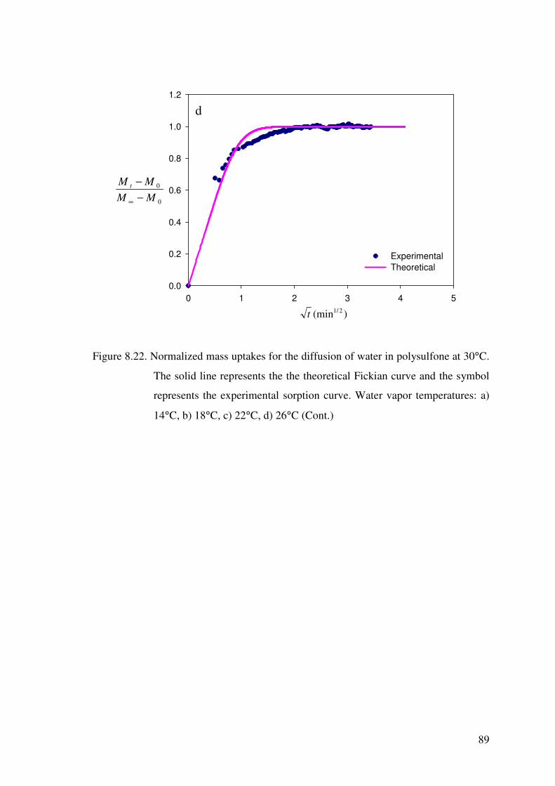
89

0 1 2 3 4 50.0

0.2

0.4

0.6

0.8

1.0

1.2


0

0

MMMM t

−−

∞

)(min 2/1t




14°C, b) 18°C, c) 22°C, d) 26°C (Cont.)

d

90

0 1 2 3 4 50.0

0.2

0.4

0.6

0.8

1.0

1.2


0

0

MMMM t

−−

∞

)(min 2/1t

0 1 2 3 4 5 60.0

0.2

0.4

0.6

0.8

1.0

1.2


0

0

MMMM t

−−

∞

)(min 2/1t




20°C, b) 25°C, c) 30°C, d) 35°C

a

b

91

0 1 2 3 4 50.0

0.2

0.4

0.6

0.8

1.0

1.2


0

0

MMMM t

−−

∞

)(min 2/1t

0 1 2 3 4 50.0

0.2

0.4

0.6

0.8

1.0

1.2


0

0

MMMM t

−−

∞

)(min 2/1t




20°C, b) 25°C, c) 30°C, d) 35°C (Cont.)

d

c

92

0 1 2 3 4 50.0

0.2

0.4

0.6

0.8

1.0

1.2


0

0

MMMM t

−−

∞

)(min 2/1t

0 1 2 3 4 50.0

0.2

0.4

0.6

0.8

1.0

1.2

1.4


0

0

MMMM t

−−

∞

)(min 2/1t




20°C, b) 25°C, c) 30°C, d) 35°C, e) 40°C, f) 45°C

b

a

93

0 1 2 3 4 50.0

0.2

0.4

0.6

0.8

1.0

1.2

1.4


0

0

MMMM t

−−

∞

)(min 2/1t

0 1 2 3 4 50.0

0.2

0.4

0.6

0.8

1.0

1.2


0

0

MMMM t

−−

∞

)(min 2/1t




20°C, b) 25°C, c) 30°C, d) 35°C, e) 40°C, f) 45°C (Cont.)

d

c

94

0 1 2 3 4 50.0

0.2

0.4

0.6

0.8

1.0

1.2


0

0

MMMM t

−−

∞

)(min 2/1t

0 1 2 3 4 50.0

0.2

0.4

0.6

0.8

1.0

1.2


0

0

MMMM t

−−

∞

)(min 2/1t




20°C, b) 25°C, c) 30°C, d) 35°C, e) 40°C, f) 45°C (Cont.)

f

e

95

The diffusivity values reported in Table 8.2 correspond to the average weight

fraction of water calculated by Equation 8.1 (Hong et al. 1998):

(8.1)

Vrentas and Duda determined that minimal error was introduced if the average

concentration was associated with 70% of the sorption interval (Vrentas and Duda

1977). Results in Figures 8.22 through 8.24 indicate that analytical solution (Equation

6.7) derived for Case 1 diffusion appropriately fits the experimental data with slight

deviation in a few cases where the data were collected at high activities. It was observed

that the initial trend in the normalized uptake data is linear with respect to t while the

latter part of the curves are concave with respect to the t axis. This result simply

suggests that sorption kinetics of water in polysulfone may follow Fickian sorption.

Table 8.2. Diffusivity data for water-polysulfone at 30°C, 40°C and 50°C

Pressure (psia) ωwater Temperature

(°C) initial Final initial equilibrium Average

thickness

(µm)

D×108

(cm2/s)

0 0.23 0 0.00406 0.00284 27.36 7.33

0.23 0.3 0.00406 0.00582 0.00529 27.5 5.19

0.3 0.38 0.00582 0.00893 0.00799 27.7 7.32 30

0.38 0.49 0.00893 0.01670 0.01458 28 11.6

0 0.34 0 0.00344 0.00240 27.36 9.82

0.34 0.46 0.00344 0.00476 0.00436 27.48 6.16

0.46 0.62 0.00476 0.00667 0.00609 27.64 9.79 40

0.62 0.82 0.00667 0.0131 0.0112 27.87 6.79

0 0.34 0 0.00217 0.00152 27.36 11.5

0.34 0.46 0.00217 0.00280 0.00261 27.43 12.2

0.46 0.62 0.00280 0.00363 0.0034 27.53 12.2

0.62 0.82 0.00363 0.00518 0.0047 27.65 11

0.82 1.07 0.00518 0.00858 0.00756 27.83 8.25

50

1.07 1.39 0.00858 0.01935 0.01612 28.13 6.77

)(7.0 initialmequilibriuinitialaverage ωωωω −+=

96

The results listed in Table 8.2 indicate that diffusivity of water in PSf does not

change strongly with the concentration of water in the film. The effect of temperature

on the diffusivities was also found to be insignificant.

The accuracy of the diffusion measurements was controlled by performing the

experiments at each temperature for 3 times. As illustrated in Figure 8.26, just for the

data collected at 50°C, reproducibility of diffusivities determined at each temperature

was found to be good.

Weight fraction of water

0.000 0.004 0.008 0.012 0.016

Diff

usiv

ity (c

m2 /s

)

10-9

10-8

10-7

10-6

Set 1Set 2Set 3

Figure 8.25. Diffusion coefficients of water in the polysulfone films as a function of its

average weight fraction for 3 sets of repeated experiments at 50°C

The diffusivity data at 40°C were also compared with those obtained by Schult

and Paul (1996a), as shown in Figure 8.19. Good agreement between two independent

data sets also confirmed the accuracy of the measurements performed in this study.

97

Regain

0.000 0.002 0.004 0.006 0.008 0.010 0.012 0.014

Diff

usiv

ity (c

m2 /s

)

10-8

10-7

10-6

Schult and Paul 199640oC-Set 1

Figure 8.26. Comparison of the diffusion coefficients with the study of Schult and Paul

(1996a). Regain is the weight of the water sorbed at the given activity by

the dry weight of the polymer.

In the study of Swinyard et al. (1990), the diffusion coefficient of water in

polysulfone was found as 7.2 × 10-8 at 40°C at unit activity which is very close to the

ones found in this study and shows the agreement of the results with the literature.

8.4.2. Determination of Diffusion Coefficients of Polysulfone/

Chloroform System

Figures 8.27 and 8.28 show gravimetric sorption curves for chloroform/PSf

system collected at 30°C and 40°C. The results are presented in terms of weight of the

chloroform absorbed, Mt-M0, versus the square root of the time. Experimental

conditions for the uptake measurements and the total thicknesses of the polymer at the

beginning of each sorption step are listed in Table 8.3.

98

0 5 10 15 20 250

100

200

300

400

500

600

700


)(0 gMM t µ−

)(min 2/1t

0 5 10 15 20 250

20

40

60

80

100

120

140


)(0 gMM t µ−

)(min 2/1t

Figure 8.27. Bouyancy corrected weight difference values as a function of t for the

diffusion of chloroform in polysulfone at 30°C. The solid line represents

the theoretical curve and the symbol represents the experimental sorption

curve. Water vapor temperatures: a) 9.9°C, b) 14°C, c) 18°C

a

b

99

0 5 10 15 20 25 30 350

100

200

300

400

500


)(0 gMM t µ−

)(min 2/1t



the theoretical curve and the symbol represents the experimental sorption

curve. Water vapor temperatures: a) 9.9°C, b) 14°C, c) 18°C (Cont.)

c

100

0 5 10 15 20 25 300

200

400

600

800


)(min 2/1t

)(0 gMM t µ−

0 2 4 6 8 10 12 140.0

0.2

0.4

0.6

0.8

1.0

1.2


)(0 gMM t µ−

)(min 2/1t



the the theoretical curve and the symbol represents the experimental

sorption curve. Chloroform vapor temperatures: a) 11.5°C, b) 25°C, c)

30.8°C, d) 36°C

a

b

101

0 2 4 6 8 10 12 14 160

100

200

300

400

500

600

700


)(min 2/1t

)(0 gMM t µ−

0 2 4 6 8 10 12 14 16 18 200

200

400

600

800

1000

1200

1400


)(min 2/1t

)(0 gMM t µ−



the the theoretical curve and the symbol represents the experimental

sorption curve. Chloroform vapor temperatures: a) 11.5°C, b) 25°C, c)

30.8°C, d) 36°C (Cont.)

c

d

102

Table 8.3. Diffusivity data for chloroform-polysulfone at 30°C and 40°C

Pressure (psia) ωchloroform Temperature

(°C) initial Final initial equilibrium average

thickness

(µm)

D×109

(cm2/s)

0 1.88 0 0.1855 0.1298 3.87 0.89

1.88 2.29 0.1855 0.2146 0.2058 4.62 2.87 30

2.29 2.76 0.2146 0.2864 0.2649 5.68 8.6

0 2.03 0 0.2233 0.1563 3.87 9.52

2.03 3.77 0.2233 0.3164 0.2885 4.81 3.83

3.77 4.81 0.3164 0.4169 0.3867 6.69 30.8 40

4.81 5.94 0.4169 0.5458 0.5071 10.72 1.16

As shown in Figures 8.27a through 8.27c, shape of the sorption curves collected

at 30°C have shown significant deviation from typical Fickian behaviour. In each case,

a two stage sorption was observed with a slight overshoot in the last sorption stage

(1.88-2.29 psia). Both two stage sorption and overshoot were considered as striking

experimental observations for diffusion of low molecular weight solutes in glassy

polymers (Kalospiros et al. 1991). For all steps, initial sorption rate is fast and increases

linearly with t which is characteristic of sorption kinetics controlled by Fickian

diffusion. At longer times, the weight increases at a much slower rate to an equilibrium

value and this stage is controlled by relaxation of the polymer chains in the glassy state

to accommodate the penetrant. Two stage sorption has also been observed for the

sorption of vinyl chloride monomer in polyvinly chloride (Berens and Hopfenberg

1978), benzene in polyethylene terephthalate (Patton et al. 1984), methyl acetate in

polymethylmethacarylate and cellulose acetate (Kishimoto et al. 1960), benzene,

toluene and ethyl benzene in polystyrene (Iwai et al. 1987, Iwai et al. 1989) and acetone

in cellulose nitrate (Kishimoto et al. 1960). In order to analyze the sorption curves, a

mathematical proposed by Berens and Hopfenberg (1978) was used. According to this

model, contributions from Fickian diffusion and relaxation processes are independent

from each other, thus, they can be considered as additive. In the first two sorption steps,

single relaxation time was used while in the last sorption step, relaxation was assumed

to take place at two different times. The model parameters, diffusion coefficient of the

penetrant (D) and the relaxation time(s) (�R), were regressed by minimizing the

103

difference between the experimental and theoretical weight uptakes calculated from

Equation 6.13. Regressed values of the diffusivities and relaxation times are listed in

Tables 8.3 and 8.4, respectively.

Table 8.4. Deborah numbers, τR and α values for chloroform-PSf at 30°C and 40°C

Tcolumn (°C) Tpenetrant (°C) De τR

9.9 97.3 16234.38

14 113 8369.73 30

18 444.91 16695.87

11.5 2679.69 42203.94

25 2680 1666.67

30.8 1.96 2337.42 40

36 1.01×10-7 9.99×10-5

The results shown in Figures 8.27a through 8.27c indicate that relaxation

diffusion model is successful in analyzing the sorption curves collected at 30°C. In

literature, overshoot phenomena observed in previous systems was attributed to solvent

induced crystallization (Overbergh et al. 1975, Vittoria 1991), development of small

microvoids (Aminabhavi and Phayde 1995, Aminabhavi et al. 1996) and slow

relaxation of the polymer chains compared to the diffusion of penetrant into the polymer

film (Etxeberria et al. 2000, Hoyt and Balik 1996, Kim et al. 1993). The overshoots

observed in this study is caused by slow relaxation of the polymer chains to their

equilibrium conformation since polysulfone used in the experiments is an amorphous

polymer. The contribution of relaxation and Fickian processes on the overall sorption

curve can be determined from the magnitudes of Deborah number. This dimensionless

number compares the time scales for mass uptakes due to structural relaxation (�R) to

the time scale for Fickian diffusion defined as L2/D where L corresponds to the

thickness of the film. The Deborah numbers calculated for each sorption step at 30°C

and 40°C are listed in Table 8.4. At T = 30°C, Deborah number was found to increase

as chloroform concentration in PSf increases. This could be attributed to presaturation

of existing available sites which results in longer relaxation periods to provide

redistribution of free volume elements, hence, to accommodate additional penetrant

(Berens and Hopfenberg, 1978).

104

The sorption curves collected at T = 40°C have also shown anomalous, i.e., non-

Fickian diffusion behavior as illustrated in Figures 8.28a through 8.28d. The data were

analyzed successfully with the relaxation diffusion model (Equation 6.13) and the

diffusivities and relaxation times regressed from these curves are listed in Tables 8.3

and 8.4, respectively. In the first step of the experiments (Figure 8.28a), an initial rapid

weight gain was followed by a two stage relaxation period, in which second relaxation

corresponds to decrease in amount of penetrant absorbed until its final equilibrium

value was reached. A transition in sorption curve from an overshoot behavior to the

two stage sorption is shown in Figure 8.28b. The shapes of the sorption curves in the

last two steps become similar to that of typical Fickian curves with a slight overshoot in

the third sequential step (Figure 8.28c). In contrast to the observation at T = 30°C, the

Deborah numbers calculated at T = 40°C were found to decrease with the increased

sorption level in the polymer. This simply indicates decreased contribution of relaxation

process on the overall sorption curve due to transition from glassy to rubbery state. To

determine the change in glass transition temperature of the polymer with absorption of

the penetrant, following equation derived by Kelly and Bueche (1961) was used:

(8.2)

In Equation 8.2, Tg1 and Tg2 are the glass transition temperature of the solvent and pure

polymer, respectively, while �s is the thermal expansion coefficient of the pure solvent.

( )( ) 11

42111

4

1108.4

1108.4

φαφφαφ

S

gSgg

TTT

+−×+−×

= −

−

105

Volume fraction of solvent

0.0 0.2 0.4 0.6 0.8 1.0

Tg (K

)

0

100

200

300

400

500

Figure 8.29. Plot of Tg as a function of volume fraction of solvent

Figure 8.29 shows that the glass transition temperature of the polymer decreases

significantly with the chloroform uptake. When the weight fractions of the chloroform

in the polymer are 0.31 and 0.33, the glass transition temperatures drop to 30°C and

40°C , respectively. As will be shown in the next section, at the last activity step of T =

30°C and T = 40°C measurements, the amount of chloroform absorbed in the polymer

was determined as 27% and 49.5% by weight, respectively. It is clear from these results

that, transition from glassy to rubbery state occurs in PSf film at T = 40°C, while the

polymer is still in glassy state at T = 30°C. Transition from glassy to rubbery state

results in relaxation of the polymer chains at a much faster rate, hence, the Deborah

numbers calculated at T = 40°C decreases with increased chloroform sorption level in

the polymer.

At T = 30°C, the diffusivity of chloform in PSf was found to increase by one

order of magnitude as the weight fraction of chloroform increased from 0.13 to 0.27.

On the other hand, at T = 40°C a decrease in diffusivity by almost one order of

magnitude was followed by an increase at the last sorption step (4.81-5.94 psia) with

significant chloroform uptake. This could be again explained by the transition from

glassy to rubbery state in PSf film.

106

8.4.3. Determination of Diffusion Coefficients of Polysulfone/Ethanol

System

Gravimetric sorption curves for ethanol/PSf system were collected at 30°C and

40°C using the films with two different thicknesses. The experimental conditions for the

first uptake measurements for PSf films with 1.5 µm initial thicknesses are listed in

Table 8.5.

0 1 2 3 4 5 6 70.0

0.2

0.4

0.6

0.8

1.0

1.2


0

0

MMMM t

−−

∞

)(min 2/1t


diffusion of ethanol in polysulfone at 30°C of Set 2. The solid line

represents the the theoretical curve and the symbol represents the

experimental sorption curve. Ethanol vapor temperatures: a) 11.9°C, b)

20°C, c) 25.6°C

a

107

0 1 2 3 4 5 6 70.0

0.2

0.4

0.6

0.8

1.0

1.2


0

0

MMMM t

−−

∞

)(min 2/1t

0 2 4 6 80.0

0.2

0.4

0.6

0.8

1.0

1.2


0

0

MMMM t

−−

∞

)(min 2/1t





20°C, c) 25.6°C (Cont.)

b

c

108

0 1 2 3 4 5 60.0

0.2

0.4

0.6

0.8

1.0

1.2

1.4


0

0

MMMM t

−−

∞

)(min 2/1t

0 1 2 3 40.0

0.2

0.4

0.6

0.8

1.0

1.2


0

0

MMMM t

−−

∞

)(min 2/1t





16.2°C, c) 20.1°C, d) 30.2°C, e) 35°C

a

b

109

0.0 0.5 1.0 1.5 2.0 2.5 3.0 3.50.0

0.2

0.4

0.6

0.8

1.0

1.2


0

0

MMMM t

−−

∞

)(min 2/1t

0 1 2 3 4 50.0

0.2

0.4

0.6

0.8

1.0

1.2


0

0

MMMM t

−−

∞

)(min 2/1t





16.2°C, c) 20.1°C, d) 30.2°C, e) 35°C (Cont.)

c

d

110

0 1 2 3 4 5 60.0

0.2

0.4

0.6

0.8

1.0

1.2


0

0

MMMM t

−−

∞

)(min 2/1t





16.2°C, c) 20.1°C, d) 30.2°C, e) 35°C (Cont.)

Table 8.5 Diffusivity data for ethanol-polysulfone at 30°C and 40°C for Set 2

Pressure (psia) ωethanol Temperature

(°C) initial Final Initial equilibrium Average

thickness

(µm)

D×1011

(cm2/s)

0 0.51 0 0.0213 0.0149 1.42 4.39

0.51 0.85 0.0213 0.0324 0.0291 1.47 10 30

0.85 1.18 0.0324 0.0552 0.0484 1.55 3.6

0 0.49 0 0.0123 0.0086 1.42 10

0.49 0.67 0.0123 0.0361 0.0290 1.45 65.57

0.67 0.85 0.0361 0.0446 0.0421 1.54 36.84

0.85 1.53 0.0446 0.060 0.0556 1.65 10.77

40

1.53 1.99 0.060 0.0708 0.0677 1.81 3.84

e

111

Figures 8.30 through 8.31 show that all curves exhibit a linear initial slope while

the latter part of the curves are concave with respect to t axis with slight overshoots

and scatter around the equilibrium values. The data are analyzed with simple Fickian

model (Equation 6.7) and diffusivities regressed from these analyses are listed in Table

8.5. At both temperatures, diffusivities increase to a maximum and then decrease.

Deviation from classical Fickian sorption has been observed when the sorption

data were collected at 30°C and 40°C with PSf films of 9.8 �m as shown in Figures

8.32 and 8.33. At both temperatures, a transition from Fickian type to two stage

sorption was observed. The curves were analyzed with the diffusion-relaxation model

(Equation 6.13) and the diffusivities and relaxation times determined from nonlinear

regression analyses are listed in Tables 8.6 and 8.7, respectively. The change in

Deborah numbers with increased ethanol uptake in the films indicate that the

contribution of relaxation process on the overall sorption increases at T = 30°C, while

opposite trend is determined at T = 40°C.

112

0 5 10 15 20 25 300

50

100

150

200

250

300


)(0 gMM t µ−

)(min 2/1t

0 5 10 15 20 25 30 350

20

40

60

80

100

120


)(0 gMM t µ−

)(min 2/1t


diffusion of ethanol in polysulfone at 30°C for Set 1. The solid line

represents model predictions and the symbol represents the experimental

sorption curve. Ethanol vapor temperatures: a) 11.7°C, b) for 15.9°C, c)

20.1°C, d) 25.1°C

b

a

113

0 10 20 30 40 500

40

80

120

160

200


)(0 gMM t µ−

)(min 2/1t

0 10 20 30 40 500

50

100

150

200

250

300


)(0 gMM t µ−

)(min 2/1t




sorption curve. Ethanol vapor temperatures: a) 11.7°C, b) for 15.9°C, c)

20.1°C, d) 25.1°C (Cont.)

c

d

114

0 2 4 6 8 10 12 14 160

20

40

60

80

100

120

140


)(0 gMM t µ−

)(min 2/1t

0 10 20 30 40 500

20

40

60

80

100

120

140

160


)(0 gMM t µ−

)(min 2/1t




sorption curve. Ethanol vapor temperatures: a) 14.3°C, b) 25°C, c) 30°C,

d) 35°C

a

b

115

0 10 20 30 40 50 60 700

50

100

150

200

250

300


)(0 gMM t µ−

)(min 2/1t

0 10 20 30 40 500

50

100

150

200

250


)(0 gMM t µ−

)(min 2/1t




sorption curve. Ethanol vapor temperatures: a) 14.3°C, b) 25°C, c) 30°C,

d) 35°C (Cont.)

c

d

116

Table 8.6. Diffusivity data for ethanol-polysulfone at 30°C and 40°C of Set 1

Pressure (psia) ωwater Temperature

(°C) Initial Final initial equilibrium average

thickness

(µm)

D×1011

(cm2/s)

0 0.5054 0 0.01579 0.01105 9.88 4.76

0.5054 0.6595 0.01579 0.02231 0.02035 10.13 6.94

0.6595 0.8529 0.02231 0.03102 0.02841 10.47 575.6 30

0.8529 1.1459 0.03102 0.04662 0.04194 10.93 659.7

0 0.5965 0 0.0081 0.00564 9.88 10.77

0.5965 1.1393 0.0081 0.01743 0.01462 10 3320

1.1393 1.5138 0.01743 0.0327 0.02815 10.21 84 40

1.5138 1.99 0.0327 0.0449 0.04125 10.65 330.7

Table 8.7 Deborah numbers, τR and α values for ethanol-polysulfone at 30°C and 40°C

Tcolumn (°C) Tpenetrant (°C) De τR

15.9 0.153 9023.04

20.1 18.62 14192.38 30

25.1 23.85 17277.66

25 137 16485.74

30 6.04 29994.14 40

35 9.98 13527.67

In order to further illustrate anomalous diffusion of ethanol in glassy PSf films,

normalized mass uptake curves were plotted against Lt

using the data measured at the

same activity levels as shown in Figures 8.34 through 8.36. Nonoverlap of two of these

curves is considered as anomalous diffusion. Infact , sample size effect is frequently

used to determine deviation from Fickian type sorption. A consequence of sample size

effect hence anomalous diffusion is reflected by the change in diffusivities with the

film thicknesses as reported in Table 8.8. At two activity steps (T = 30°C, a = 0.56 and

T = 40°C, a = 0.76) diffusivities vary from each other by two orders of magnitude while

similar diffusivities were determined for the activity level of 0.33 at T = 30°C.

117

0 10000 20000 30000 40000 500000.0

0.2

0.4

0.6

0.8

1.0

1.2

Set 1 a = 0.334Set 2 a = 0.338

0

0

MMMM t

−−

∞

)/(min 2/1 cmLt

Figure 8.34. Plot of Mt/M∞ as a function of Lt at activity = 0.33 for different

thicknesses

0 5000 10000 15000 20000 25000 30000 350000.0

0.2

0.4

0.6

0.8

1.0

1.2

Set 1 a = 0.76Set 2 a = 0.76

0

0

MMMM t

−−

∞

)/(min 2/1 cmLt


thicknesses

30°°°°C

40°°°°C

118

0 10000 20000 30000 40000 500000.0

0.2

0.4

0.6

0.8

1.0

1.2

Set 1 a = 0.56Set 2 a = 0.56

0

0

MMMM t

−−

∞

)/(min 2/1 cmLt


thicknesses

Table 8.8. Diffusion coefficients of ethanol in PSf as a function of the film thickness

L (µm) Activity D×10-11

9.88 0.334 4.76

1.486 0.338 4.39

9.88 0.56 575.6

1.486 0.56 3.6

9.88 0.76 330.7

1.486 0.76 3.84

8.4.4. Equilibrium Isotherms of Penetrants in Polysulfone

Sorption isotherm of a penetrant in a polymer is usually plotted as activity of the

penetrant in the vapor phase against its volume fraction in the polymer. By assuming

that the penetrant vapor is ideal, activity was calculated from the ratio of the saturation

vapor pressure of the penetrant at the penetrant temperature to that at column

temperature as given below.

30°°°°C

119

(8.3)

For all penetrants, the weight fraction gravimetric sorption data were converted

to volume fractions and the results are given in Tables 8.9 through 8.11 for water,

ethanol and chloroform, respectively. Figure 8.37 illustrates the repeatability of the

experiments with the sorption isotherm of water collected at T = 50°C.

Table 8.9. Sorption isotherms for water in polysulfone measured at the column

temperatures 30°C, 40°C and 50°C

T(°C) Volume Fraction of Water Activity

0.005031 0.377

0.007209 0.486

0.011045 0.623 30

0.020991 0.792

0.004259 0.317

0.005898 0.430

0.008251 0.575 40

0.016236 0.762

0.002688 0.190

0.003473 0.257

0.004495 0.344

0.006407 0.456

0.010611 0.598

50

0.023881 0.777

)(

)(

1

1

column

penetrant

TP

TPActivity

�

�

=

120

Volume fraction of water

0.000 0.005 0.010 0.015 0.020 0.025

Act

ivity

0.0

0.2

0.4

0.6

0.8

1.0

Set 1Set 2Set 3

Figure 8.37. Sorption isotherms for 3 sets of repeated experiments at 50°C

Table 8.10. Sorption isotherms for chloroform in polysulfone measured at the column

temperatures 30°C and 40°C

T(°C) Volume Fraction of Chloroform Activity

0.1611 0.404

0.1873 0.492 30

0.2529 0.593

0.1951 0.293

0.2808 0.809

0.3762 0.694 40

0.5034 0.856

121

Table 8.11. Sorption isotherms for ethanol in polysulfone measured at the column

temperatures 30°C and 40°C

T(°C) Volume Fraction of Ethanol Activity

0.02447 0.334

0.03445 0.436

0.04767 0.563 30

0.07103 0.757

0.01254 0.230

0.02698 0.44

0.05027 0.585 40

0.06846 0.769

8.5. Modeling of Diffusion and Equilibrium Studies

8.5.1. Modeling of the Equilibrium Isotherm

8.5.1.1. Modeling of the Equilibrium Isotherm of Water/PSf System

Equilibrium sorption isotherms of water/PSf system measured at 30°C, 40°C and

50°C were not correlated well with a constant interaction parameter. Thus, following

expression for concentration dependence of the Flory Huggins interaction parameter

was proposed:

(8.4)

where a0 and a1 are empirical constants. These two constants were evaluated

using the sorption data collected at 30°C, 40°C and 50°C, and were found to be -13.69

and 17.18, respectively. Figure 8.38 shows that Flory Huggins theory along with

proposed concentration dependence of the Flory-Huggins interaction parameter

successfully correlates the sorption isotherms of water/PSf system. The average value of

the Flory Huggins interaction parameter within the volume fraction range from 0 to 1

was determined as 3.15. The value of average χ greater than 0.5 simply indicates that

water acts as a nonsolvent for PSf.

210 φχ aa +=

122

Volume fraction of water

0.000 0.005 0.010 0.015 0.020 0.025 0.030

Act

ivity

0.0

0.2

0.4

0.6

0.8

1.0

30 oC40 oC50 oCFlory Huggins Model

Figure 8.38. Sorption isotherm of water-polysulfone system

8.5.1.2. Modeling of the Equilibrium Isotherm of Chloroform/PSf

System

Equilibrium sorption isotherms of chloroform/PSf system measured at 30°C and

40°C were correlated well with a constant Flory Huggins interaction parameter as

shown in Figure 8.39. From the nonlinear regression analysis, the Flory Huggins

interaction parameter was determined as -0.03. The negative sign of the χ parameter

indicates strong interaction between polysulfone and chloroform. In addition, very small

value of χ compared to the limiting value of 0.5 simply proves that chloroform is a very

good solvent for polysulfone.

123

Volume fraction of chloroform

0.0 0.2 0.4 0.6 0.8

Act

ivity

0.0

0.2

0.4

0.6

0.8

1.0

30 oC40 oCFlory Huggins Model

Figure 8.39. Sorption isotherm of chloroform-polysulfone system

8.5.1.3. Modeling of the Equilibrium Isotherm of Ethanol/PSf System

Equilibrium sorption isotherms of ethanol/PSf system measured at 30°C and

40°C were correlated well with a constant interaction parameter as shown in Figure

8.40. By minimizing the difference between the experimental data points and theoretical

values, the Flory Huggins interaction parameter between ethanol and polysulfone was

determined as 1.76. This value is close to the one obtained from swelling experiments as

1.8. The role of ethanol as nonsolvent for the production of PSf membranes is

confirmed by the value of χ parameter greater than 0.5. The interaction parameter of

water larger than that of ethanol simply indicates greater nonsolvent power of water for

polysulfone. In other words, the homogeneous phase region is enlarged when ethanol

rather than water is used as nonsolvent as shown in Figure 8.10.

124

Volume fraction of ethanol

0.00 0.02 0.04 0.06 0.08 0.10

Act

ivity

0.0

0.2

0.4

0.6

0.8

1.0

1.2

30C40CFlory Huggins Model

Figure 8.40. Sorption isotherm of ethanol-polysulfone system

8.5.2. Correlation and Prediction of Diffusion Coefficients

8.5.2.1. Correlation and Prediction of Diffusion Coefficients of

Water/PSf system

The diffusivities of water in polysulfone were correlated with Vrentas and Duda

free volume theory (Vrentas and Duda 1979). The equation used for the correlation is

described by Equation 3.9 and the unknown parameters D0 and ξ were obtained by

fitting the experimental data collected at 30°C and 40°C and minimizing the following

objective function using solver tool in Excel.

(8.5)

The other free volume parameters required in Equation 3.9 were taken from the

study of Yip et al. (2006) and Alsoy Altinkaya and Ozbas (2004). The free volume

parameters along with the regressed parameters, D0 and ξ are listed in Table 8.12.

( ) =

−dataN

iltheoreticaerimental DD

1

2exp lnlnmin

125

Table 8.12. Free volume parameters of polysulfone and water

(Source: a Yip et al. 2006, b Alsoy and Ozbas 2004)

Parameter PSf/water

K11/γ (cm3/gK) 0.00218b

K12/γ (cm3/gK) -152.29b

K21-Tg1 (K) 0.00043a

K22-Tg2 (K) -410a

∗1̂V (cm3/g) 1.071b

∗2V̂ (cm3/g) 0.733a

D0 (cm2/s) 1.584×10-7 b

ξ 0.741b

Figure 8.41 shows that diffusivities calculated from Equation (3.14) by using the

parameters listed in Table 8.12 are in agreement with the experimental ones. This

agreement indicates that Vrentas and Duda free volume theory can correlate the

diffusion behavior of water in polysulfone at 30°C and 40°C. Diffusivities obtained

experimentally at 50°C are very close to the ones measured at 40°C, as a result it was

observed that Vrentas and Duda free volume theory can not correlate the diffusion

behavior at 50°C.

126

Weight fraction of water

0.000 0.003 0.006 0.009 0.012 0.015 0.018

D (c

m2 /s

)

10-9

10-8

10-7

10-6

30 oC40 oC

Figure 8.41. Experimental and correlated diffusivities with respect to weight fraction of

water. The symbols represent the experimental data while the lines

correspond to the free volume correlation.

127

CHAPTER 9

CONCLUSIONS

In this study, experimental cloud points for PSf/NMP (1-methyl-2-

pyrrolidinone)/water, PSf/THF (Tetrahydrofuran)/water, PSf/NMP/ethanol,

PSf/THF/water, PMMA (Polymethylmethacrylate)/acetone/water, PMMA/THF/water,

PMMA /acetone/formamide and PMMA/THF/formamide systems were determined by

the titration of homogeneous polymer solutions with nonsolvents until the onset of

turbidity. In addition, sorption isotherms and diffusivity of water, ethanol and

chloroform in polysulfone were measured by a gravimetric sorption technique.

The cloud point measurements have shown that the region of the homogeneous

phase is slightly larger in the PSf/NMP/water system than in the PSf/THF/water system

at the same temperature. The influence of solvent type on the cloud points become more

pronounced when ethanol is used as a nonsolvent. It was observed that homogeneous

phase region is larger in the PSf/NMP/ethanol than in the PSf/THF/ethanol system at

40°C. This indicates that nonsolvent power of water is higher than that of ethanol for

PSf films. For the case of PMMA, the homogeneous phase region is not influenced by

solvent type which are acetone and THF when both water and formamide are used as

nonsolvents. The nonsolvent power of water is higher than formamide when acetone

and THF are used as solvents. It has been observed that the effect of temperature on the

cloud points is relatively small. By using the numerical code developed, the theoretical

ternary phase diagrams of PSf/NMP/water, PSf/THF/water, PSf/NMP/ethanol,

PSf/THF/ethanol, PMMA/acetone/water and PMMA/THF/water were constructed and

very good agreement was obtained between the theoretical and experimental results for

the systems PSf/NMP/water, PSf/THF/water, PSf/NMP/ethanol and PSf/THF/ethanol.

For the systems, PMMA/acetone/water and PMMA/THF/water, the experimental cloud

points didn’t agree well with the theoretical binodal curves. These results can be

explained by the inaccuracies in interaction parameters obtained from different sources.

For polysulfone/water system, sorption kinetics follows Fickian sorption. Analytical

solution derived for Case 1 diffusion appropriately fits the experimental data of

polysulfone/water system with slight deviation in a few cases where the data were

collected at high activities. For the case of polysulfone/chloroform system, almost in

128

each case two stage sorption with a slow relaxation is observed. In a few cases,

overshoot due to slow relaxation of polymer chains is noted. These kinetic behaviors are

successfully modeled with diffusion-relaxation model. In PSf/ethanol system, Fickian

type sorption is observed with the films of 1.5 µm, while two-stage sorption is seen

when the film thickness is around 10 µm. The sample size effect observed for this

system is attributed to relaxation of polymer chains in their glassy state.

Flory Huggins theory along with proposed concentration dependence of the

Flory-Huggins interaction parameter successfully correlates the sorption isotherms of

PSf/water system while for the polysulfone/ethanol and polysulfone/chloroform

systems, Flory Huggins theory with constant interaction parameter is used. The Flory

Huggins interaction parameter for Chloroform/PSf system is determined as -0.03 which

indicates strong interaction between PSf and chloroform. The interaction parameter of

water is found larger than that of ethanol which confirms greater nonsolvent power of

water for PSf.

Experimental diffusivities of water in PSf collected at 30°C and 40°C is

successfully correlated with Vrentas and Duda free volume theory. On the other hand,

the theory fails to correlate the diffusivity data for chloroform/PSf and ethanol/PSf

systems.

129

REFERENCES

Alentiev, A., Sanopoulou, M., Ushakov, N., Papadokostaki, K.G. 2002. “Melting and

Recrystallization Processes in a Rubbery Polymer Detected by Vapor Sorption

and Temperature-Modulated DSC Methods”, Polymer. Vol. 43, p.1949.

Alfageme, J.A., Iriarte, M., Iruin, J.J., Etxeberria, A., Uriarte, C. 1999. “Water-

Transport Properties in Polyetherimide Blends with a Liquid Crystal Polymer”,

Journal of Applied Polymer Science. Vol. 73, p. 323.

Allen, G., McAinsh, J., Strazielle, C. 1969. “Dilute Solution Properties of the Polyether

From Bisphenol ‘A’ and 4,4 Dichlorodiphenyl Sulphone”, European Polymer

Journal. Vol. 5, p. 319.

Alsoy Altinkaya, S., Ozbas, B. 2004. “Modeling of Asymmetric Membrane Formation

by Dry-casting Method”, Journal of Membrane Science. Vol. 230, p. 71.

Altena, F.W., Smolders, C.A. 1982. “Calculation of Liquid-Liquid Phase Separation in

a Ternary System of a Polymer in a Mixture of a Solvent and a Nonsolvent”,

Macromolecules. Vol. 15, p. 1491.

Aminabhavi, T.M., Phayde, H.T.S. 1995. “Molecular Transport Characteristics of

Santoprene Thermoplastic Rubber in the Presence of Aliphatic Alkanes Over the

Temperature Interval of 25 to 70°C”, Polymer. Vol. 36, p. 1023.

Aminabhavi, T.M., Phayde, H.T.S., Ortego, J.D. 1996. “Resistivity and Dimensional

Stability of High-performance Engineering Thermoplastic Blend of Ethylene-

propylene Random Copolymer and Isotactic Polypropylene Membrane in the

Presence of Hazardous Haloalkanes”, Journal of Hazardous Materials. Vol. 46, p.

71.

130

Areerat, S., Hayata, Y., Katsumoto, R., Kegasawa, T., Egami, H., Ohshima, M. 2002.

“Solubility of Carbon Dioxide in Polyethylene/Titanium Dioxide Composite

Under High Pressure and Temperature”, Journal of Applied Polymer Science.

Vol. 86, p. 282.

Balashova, I.M., Danner, R.P., Puri, P.S., Duda, J.L. 2001. “Solubility and Diffusivity

of Solvents and Nonsolvents in Polysulfone and Polyetherimide”, Industrial &

Engineering Chemistry Research. Vol. 40, p. 3058.

Barth, C., and Wolf, B.A. 2000. “Quick and Realiable Routes to Phase Diagrams for

Polyethersulfone and Polysulfone Membrane Formation”, Macromolecular

Chemistry and Physics. Vol. 201, No.3, p. 365.

Baschetti, M.G., Piccinini, E., Barbari, T.A., Sarti, G.C. 2003. “Quantitative Analysis of

Polymer Dilation During Sorption Using FTIR-ATR Spectroscopy”,

Macromolecules. Vol. 36, p. 9574.

Bearman, R.J. 1961. “On the Molecular Basis of Some Current Theories of Diffusion”,

Journal of Physical Chemistry. Vol. 65, p. 1961.

Berens, A.R., Hopfenberg, H.B. 1978. “Diffusion and Relaxation in Glassy Polymer

Powders: 2. Separation of Diffusion and Relaxation Parameters”, Polymer. Vol.

19, p. 489.

Brandrup, J., Immergut, E.H., Grulke, E.A., 1999. Polymer Handbook, (John Wiley &

Sons Inc.)

Bristow, G.M., Watson, W.F. 1958. “Cohesive Energy Densities of Polymers: Part 1.-

Cohesive Energy Densities of Rubbers by Swelling Measurements”, Trans.

Faraday Society. Vol. 54., p. 1731.

Chang, S-M., Muramatsu, H., Nakamura, C., Miyake, J. 2000. “The Principle and

Applications of Piezoelectric Crystal Sensors”, Materials Science and

Engineering. Vol. C 12, p. 111.

131

Chaudhary, B.I., Johns, A.I. 1998. “Solubilities of Nitrogen, Isobutane and Carbon

Dioxide in Polyethylene”, Journal of Cellular Plastics. Vol. 34, p. 312.

Cheng, J-M., Wang, D-M., Lin, F-C., Lai, J-Y. 1996. “Formation and Gas Flux of

Asymmetric PMMA Membranes”, Journal of Membrane Science. Vol. 109, p. 93.

Chin, J.W., Nguyen, T., Aouadi, K. 1999. “Sorption and Diffusion of Water, Salt Water,

and Concrete Pore Solution in Composite Materials”, Journal of Applied Polymer

Science. Vol. 71, p.483.

Cohen, M.H., Turnbull, D. 1959. “Molecular Transport in Liquids and Glasses”,

Journal of Chemical Physics. Vol. 31, p. 1164.

Crank, J., 1975. The Mathematics of Diffusion, Third Edition, (Oxford Science

Publications, Oxford), p.2.

Crank, J., Park, G.S., 1968. “Methods of Measurement”, in Diffusion in Polymers,

(Academic Press Inc., New York), p.1.

Danner, R.P., High, M.S., 1993. Handbook of Polymer Solution Thermodynamics,

(American Institute of Chemical Engineers, New York).

Davis, P.K., Danner, R.P., Duda, J.L., Romdhane, I.H. 2004a. “Use of Inverse Gas

Chromatography to Study Binary Polymer-Solvent Systems Near The Glass

Transition Temperature”, Macromolecules, Vol. 37, p. 9201.

Davis, P.K., Lundy, G.D., Palamara, J.E., Duda, J.L., Danner, R.P. 2004b. “New

Pressure-Decay Techniques to Study Gas Sorption and Diffusion in Polymers at

Elevated Pressures”, Industrial & Engineering Chemical Research. Vol. 23, p.

1537.

Daubert, T.E., Danner, R.P., 1994. Physical and Thermodynamic Properties of Pure

Compounds: Data Compilation, (Taylor&Francis, New York).

132

Dhoot, S.N., Freeman, B.D., Stewart, M.E., Hill, A.J. 2001. “Sorption and Transport of

Linear Alkane Hydrocarbons in Biaxially Oriented Polyethylene Terephthalate”,

Journal of Polymer Science: Part B: Polymer Physics. Vol. 39, p. 1160.

Dhoot, S.N. 2004. “Sorption and Transport of Gases and Organic Vapors in

Polyethylene Terephthalate”, M.S. Thesis. The University of Texas in Austin.

Doghieri, F., Biavati, D., Sarti, G.C. 1996. “Solubility and Diffusivity of Ethanol in

PTMSP: Effects of Activity and of Polymer Aging”, Industrial & Engineering

Chemistry Research. Vol. 35, p. 2420.

Doolittle, A.K. 1951. “Studies in Newtonian Flow. II. The Dependence of the Viscosity

of Liquids on Free-Space”, Journal of Applied Physics. Vol. 22, p. 1471.

Dreisbach, F., Staudt, R., Keller, J.U. 1998. “Experimental Investigation of the Kinetics

of Adsorption of Pure Gases and Binary Mixtures on Activated Carbon” in

Fundamentals of Adsorption 6, F. Meunier Edition, (Elsevier), p. 279.

Dreisbach, F., Lösch, H.W. 2000. “Magnetic Suspension Balance For Simultaneous

Measurements of a Sample and the Density of the Measuring Fluid”, Journal of

Thermal Analysis and Calorimetry. Vol. 62, p. 515.

Dreisbach, F., Seif, R.A.H., Lösch, H.W. 2002. “Gravimetric Measurements of

Adsorption Equilibria of Gas Mixture CO/H2 with a Magnetic Suspension

Balance”, Chemical Engineering Technology. Vol. 25, p. 1060.

Dubreil, A-C., Doumenc, F., Guerrier, B., Johannsman, D., Allain, C. 2003. “Analysis

of the Solvent Diffusion in Glassy Polymer Films Using a Set Inversion Method”,

Polymer. Vol. 44, p. 377.

Duda, J.L., Vrentas, J.S., Ju, S.T., Liu, H.T. 1982. “Prediction of Diffusion Coefficients

for Polymer-Solvent Systems”, AlChE Journal. Vol. 28, p. 279.

133

Dullien, F.A.L. 1972. “Predictive Equations for Self-Diffusion in Liquids: A Different

Approach”, AlChE Journal. Vol. 18, p. 62.

Etxeberria, A., Etxabarren, C., Iruin, J.J. 2000. “Comparison Between Static (Sorption)

and Dynamic (IGC) Methods in the Determination of Interaction Parameters in

Polymer/Polymer Blends”, Macromolecules. Vol. 33, p. 9115.

Feng, J. 2001. “Interaction and Permeability of Water with Liquid Crystalline

Thermoset”, PhD Thesis. University of Florida.

Ferry, J.D., 1970. Viscoelastic Propoerties of Polymers, Second Edition, (Wiley, New

York).

Fried, J.R., 1995. Polymer Science and Technology, Third Edition, (Prentice Hall PTR

Englewood Cliffs, New Jersey).

Flory, P.J., 1985. Principles of Polymer Chemistry, (Cornell University Press, Ithaka,

New York).

Ghi, P., Hill, D.J.T., Whittaker, A.K. 2000. “Water Sorption by Poly(tetrahydrofurfuryl

methacrylate-co- 2-hydroxyethyl methacrylate). I. A Mass-Uptake Study”,

Journal of Polymer Science: Part B: Polymer Physics. Vol. 38, p. 1939.

Han, M-J. 1999. “Effect of Propionic Acid in the Casting Solution on the Characteristics

of Phase Inversion Polysulfone Membranes”, Desalination. Vol. 121, p.31.

Haward, R.N. 1970. “Occupied Volume of Liquids and Polymers”, Journal of

Macromolecular Science-Reviews in Macromolecular Chemistry. C4, p. 191.

Hazeleger, M.C. 2006. “Understanding Adsorption in Micropores, a Study of Carbons,

Soils and Zeolites”, M.S. Thesis. Universiteit van Amsterdam.

Hong, S-U. 1995. “Prediction of Polymer/Solvent Diffusion Behavior Using Free-

Volume Theory”, Industrial&Engineering Chemistry Research. Vol. 34, p. 2536.

134

Hong, S.U., Laurer, J.H., Zielinski, J.M., Samseth, J., Smith, S.D., Duda, J.L., Spontak,

R.J. 1998. “Morphological and Isothermal Diffusive Probe Analyses of Low

Molecular-Weight Diblock Copolymers”, Macromolecules. Vol. 31, p. 2174.

Hopfenberg, H.B., Frisch, H.L. 1969. “Transport of Organic Micromolecules in

Amorphous Polymers”, Journal of Polymer Physics: Part B. Polymer Letters.

Vol. 7, p. 405.

Hoyt, M.A., Balik, C.M. 1996. “Diffusivity of a Drug Preservative in Bromobutyl

Rubber”, Polymer Engineering and Science. Vol. 36, No.14, p.1862.

Huang, Y., Liu, H., Hu, Y. 2003. “Transport of Mixed Solvents in Glassy Polymer

Membrane”, Journal of Membrane Science. Vol. 222, p. 123.

Iwai, Y., Kohno, M., Akiyama, T., Arai, Y. 1987. “Measurement and Correlation of

Mutual Diffusion Coefficients for Molten Polystyrene-Hydrocarbon Systems”,

Polymer Engineering Science. Vol. 27, p. 837.

Iwai, Y., Maruyama, S., Fujimoto, M., Miyamoto, S., Arai, Y. 1989. “Measurement and

Correlation of Mutual Diffusion Coefficients for Polybutadiene-Hydrocarbon

Systems”, Polymer Engineering Science. Vol. 29, p. 773.

Ju, S.T., Duda, J.L., Vrentas, J.S. 1981a “Influence of Temperature on the Diffusion of

Solvents in Polymers Above the Glass Transition Temperature”, Industrial &

Engineering Chemistry Product Research and Development. Vol. 20, p.330.

Ju, S.T., Liu, H.T., Duda, J.L., Vrentas, J.S. 1981b. “Solvent Diffusion in Amorphous

Polymers”, Journal of Applied Polymer Science. Vol. 26, p. 3735.

Kalospiros, N.S., Ocone, R., Astarita, G., Meldon, J.H. 1991. “Analysis of Anomalous

Diffusion and Relaxation in Solid Polymers”, Industrial & Engineering Chemistry

Research. Vol. 30, p. 851.

135

Kamaruddin, H.D., Koros, W.J. 2000. “Experimental Procedure Utilizing Extraction

and Head-Space Analytical Method For Obtaining Methanol/MTBE Mixed-

Liquid Sorption Isotherms in a Glassy Polymer”, Journal of Polymer Science Part

B: Polymer Physics. Vol. 38, p. 2268.

Karimi, M., Albrecht, W., Heuchel, M., Kish, M.H., Frahn, J., Weigel, Th., Hofmann,

D., Modarress, H., Lendlein, A. 2005. “Determination of Water/Polymer

Interaction Parameter For Membrane-Forming Systems by Sorption Measurement

and a Fitting Technique”, Journal of Membrane Science. Vol. 265, p. 1.

Kelly, F.N., Bueche, F. 1961. “Viscosity and Glass Temperature Relations for Polymer-

Diluent Systems”, Journal of Polymer Science. Vol. 50, p. 549.

Kim, D., Caruthers, J.M., Peppas, N.A. 1993. “Penetrant Transport in Crosslinked

Polystyrene”, Macromolecules. Vol. 26, p. 1841.

Kim, J.Y., Lee, H.K., Baik, K.J., Kim, S.C. 1997. “Liquid-Liquid Phase Separation in

Polysulfone/Solvent/Water Systems”, Journal of Applied Polymer Science. Vol.

65, p. 2643.

Kim, J.H., Min, B.R., Won, J., Park, H.C., Kang, Y.S. 2001. “Phase Behavior and

Mechanism of Membrane Formation for Polyimide/DMSO/Water System”,

Journal of Membrane Science. Vol. 187, p. 47.

Kishimoto, A., Fujita, H., Odani, H., Kurata, M., Tamura, M. 1960. “Successive

Differential Absorptions of Vapors by Glassy Polymers”, Journal of Physical

Chemistry. Vol. 64, p. 594.

Kleinrahm, R., Wagner, W. 1986. “Measurement and Correlation of the Equilibrium

Liquid and Vapour Densities and Vapour Pressure Along the Coexistence Curve

of Methane”, Journal of Chemical Thermodynamics. Vol. 18, p. 739.

Krüger, K-M., Sadowski, G. 2005. “Fickian and Non-Fickian Sorption Kinetics of

Toluene in Glassy Polystyrene”, Macromolecules. Vol. 38, p. 8408.

136

Krüger, K-M., Pfohl, O., Dohrn, R., Sadowski, G. 2006. “Phase Equilibria and

Diffusion Coefficients in the Poly (dimethyl siloxane) + n-Pentane System”, Fluid

Phase Equilibria. Vol. 241, p. 138.

Kwapinski, W., Tsotsas, E. 2004. “Determination of Kinetics and Equilibria For

Adsorption of Water Vapor on Single Zeolite Particles by a Magnetic Suspension

Balance”, Chemical Engineering Technology. Vol. 27, p. 681.

Lai, J-Y., Lin, S-F., Lin, F-C., Wang, D-M. 1998. “Construction of Ternary Phase

Diagrams in Nonsolvent/Solvent/PMMA Systems”, Journal of Polymer Science:

Part B: Polymer Physics. Vol. 36, p. 607.

Magnetic Suspension Balances, Setup Manuel, Rubotherm Präzisionsmesstechnil Gmbh

Mamaliga, I., Schabel, W., Kind, M. 2004. “Measurement of Sorption Isotherms and

Diffusion Coefficients by Means of a Magnetic Suspension Balance”, Chemical

Engineering and Processing. Vol. 43, p. 753.

Mark, H.F., 2004. “Polysulfones”, in Encyclopedia of Polymer Science and Technology,

(John Wiley, New York), Vol. 4, p. 1.

McDonough, L.A. 2004. “Microscopy and Spectroscopy of Water Uptake in Polymer

Photoresists”, PhD Thesis. University of Colorado.

McDowell, C.C. 1998. “Sorption and Transport of Acetone in Random Copolymers of

Poly(ethylene terephthalate) and Poly(ethylene 2.6-naphthalate)”, PhD Thesis.

North Carolina State University.

Mohammadi, R.P. 2005. “Mechanism of Bubble Formation During the Drying of

Polymer Films”, PhD Thesis. The Pennsylvania State University.

Nalawade, S.P., Picchioni, F., Janssen, L.P.B.M., Patil, V.E., Keurentjes, J.T.F., Staudt,

R. 2006. “Solubilities of Sub- and Supercritical Carbon Dioxide in Polyester

Resins”, Polymer Engineering and Science. Vol. 46, p. 643.

137

O�uzer Ö. 2005. “Screening and Characterization of Catalytic Composite Membranes

for Ethylacetate Production”, Master of Science Thesis. Middle East Technical

University, Ankara.

Overbergh, N., Berghmans, H., Smets, G. 1975. “Crystallization of Isotactic

Polystyrene Induced by Organic Vapors”, Polymer. Vol. 16, p. 703.

Ozbas, B. 2001. “Modeling of Asymmetric Membrane Formation by Dry Casting

Method”, Master of Science Thesis. �zmir Institute of Technology, �zmir.

Patton, C.J., Felder, R.M., Koros, W.J. 1984. “Sorption and Transport of Benzene in

Poly(ethylene terephthalate), Journal of Applied Polymer Science. Vol. 29, p.

1095.

Pawlisch, C.A., Macris, A., Laurence, R.L. 1987. “Solute Diffusion in Polymers. 1. The

Use of Capillary Column Inverse Gas Chromatography”, Macromolecules, Vol.

20, p. 1564.

Piccinini, E., Baschetti, M.G., Sarti, G.C. 2004. “Use of an Automated Spring Balance

For the Simultaneous Measurement of Sorption and Swelling in Polymeric

Films”, Journal of Membrane Science. Vol. 234, p. 95.

Pfannschmidt, O., Michaeli, W. 1998. “Determination of the Solubility and Diffusivity

of Gases in Polymers by Using a High-Pressure Magnet-Suspension-Balance”,

Proceedings of the Annular Technical Conference of the Society of Plastics

(ANTEC), Atlanta, USA, p. 1918.

Rautenbach, R., Albrecht, R., 1989. Membrane Processes, Third Edition, (John Wiley

and Sons, Chichester).

Rodriguez, O., Fornasiero, F., Arce, A., Radke, C.J., Prausnitz, J.M. 2003. “Solubilities

and Diffusivities of Water Vapor in Poly(methylmethacrylate), Poly(2-

hydroxyethylmethacrylate), Poly(N-vinyl-2-pyrrolidone) and Poly(acrylonitrile)”,

Polymer. Vol. 44, p. 6323.

138

Romdhane, I.H. 1994. “Polymer-Solvent Diffusion and Equilibrium Parameters by

Inverse Gas-Liquid Chromatography”, PhD Thesis. The Pennsylvania State

University.

Saby-Dubreuil, A.-C., Guerrier, B., Johannsmann, D. 2001. “Glas Transition Induced by

Solvent Desorption For Statistical MMA/nBMA Copolymers-Influence of

Copolymer Composition”, Polymer. Vol. 42, p. 1383.

Saleh, B., Wendland, M. 2005. “Measurements of Vapor Pressures and Saturated Liquid

Densities of Pure Fluids with a New Apparatus”, Journal of Chemical

Engineering Data. Vol. 50, p. 429.

Sato, Y., Takikawa, T., Takishima, S., Masuoka, H. 2001. “Solubilities and Diffusion

Coefficients of Carbon Dioxide in Poly(vinyl acetate) and Polystyrene”, Journal

of Supercritical Fluids. Vol. 19, p. 187.

Schneider, A., Wünsch, M., Wolf, B.A. 2002. “An Apparatus for Automated Turbidity

Titrations and Its Application to Copolymer Analysis and to the Determination of

Phase Diagrams”, Macromolecules. Vol. 203, p. 705.

Schnitzler, J.V., Eggers, R. 1999. “Changing Properties of Glassy Polymers Due to

Diffusion of Supercritical CO2”, High Pressure Chemical Engineering,

Proceedings of the International Meeting of the GVC-Fachausschuβ

Hochdruckverfahrenstechnik, Karlsruhe, Germany, p. 57.

Schuhmacher, E., Soldi, V., Pires, A.T.N. 2001. “PMMA or PEO in THF/H2O Mixture:

Phase Diagram, Separation Mechanism and Application”, Journal of Membrane

Science. Vol. 184, p. 187.

Schult, K.A. and Paul, D.R. 1996a. “Water Sorption and Transport in a Series of

Polysulfones”, Journal of Polymer Science: Part B: Polymer Physics. Vol. 34, p.

2805.

139

Schult, K.A. and Paul, D.R. 1996b. “Techniques for Measurement of Water Vapor

Sorption and Permeation in Polymer Films”, Journal of Applied Polymer Science.

Vol. 61, p. 1865.

Subrahmanyan, S. 2003. “An Investigation of Pore Collapse in Asymmetric Polysulfone

Membranes”, PhD Thesis. Virginia Polytechnic Institute and State University.

Sugden, S. 1927. “Molecular Volumes at Absolute Zero. Part II. Zero Volumes and

Chemical Composition”, Journal of Chemical Society. p.1786

Surana, R.K., Danner, R.P., Tihminlioglu, F., Duda, J.L. 1996. “Evaluation of Inverse

Gas Chromatography For Prediction and Measurement of Diffusion Coefficients”,

Journal of Polymer Science: Part B:Polymer Physics. Vol. 35, p. 1233.

Swinyard, B.T., Sagoo, P.S., Barrie, J.A., Ash, R. 1990. “The Tranport and Sorption of

Water in Polyethersulphone, Polysulphone, and Polyethersulphone/Phenoxy

Blends”, Journal of Applied Polymer Science. Vol. 41, p. 2479.

Tihminlioglu, F., Danner, R.P. 2000. “Solvent Diffusion in Amorphous Polymers:

Polystyrene-Solvent Systems”, Journal of Polymer Science: Part B: Polymer

Physics. Vol. 38, p. 1965.

Tihminlioglu, F., Danner, R.P., Lützow, N., Duda, J.L. 2000. “Solvent Diffusion in

Amorphous Polymers: Polyvinyl Acetate-Toluene System”, Journal of Polymer

Science: Part B: Polymer Physics. Vol. 38, p. 2429.

Tompa, H., 1956. Polymer Solutions, (Butterworths, London).

Tsai, H-A., Ruaan, R-C., Wang, D-M., Lai, J-Y. 2002. “Effect of Temperature and Span

Series Surfactant on the Structure of Polysulfone Membranes”, Journal of Applied

Polymer Science. Vol. 86, p. 166.

140

Tweddle, T.A., Kutowy, O., Thayer, W.L., Sourirajan, S. 1983. “Polysulfone

Ultrafiltration Membranes”, Industrial and Enginnering Chemistry Product

Research and Development. Vol. 22, p. 320.

Tung, K-L., Lu, K-T., Ruaan, R-C., Lai, J-Y. 2006. “Molecular Dynamics Study of the

Effect of Solvent Types on the Dynamic Properties of Polymer Chains in

Solution”, Desalination. Vol. 192, p.380.

Uriarte, C., Alfageme, J., Iruin, J.J. 1998. “Carbon Dioxide Transport Properties of

Composite Membranes of a Polyetherimide and a Liquid Crystal Polymer”,

European Polymer Journal. Vol. 34, p. 1405.

van der Wel, G.K., Adan, O.C.G. 1999. “Moisture in Organic Coatings-A Review”,

Progress in Organic Coatings. Vol. 37, p. 1.

van de Witte, P., Dijkstra, P.J., van den Berg, J.W.A., Feijen, J. 1996. “Phase Separation

Processes in Polymer Solutions in Relation to Membrane Formation”, Journal of

Membrane Science. Vol. 117, p. 1

Vittoria, V. 1991. “Solvent-Induced Crystallization of Isotactic Polypropylene in

Cyclohexane at Different Temperatures”, Polymer. Vol. 32, p. 856.

Vogel, H. 1921. “Das Temperaturabhangigkeitsgesetz Auf die Viscositat von

Flussigkeiten”, Physik. Vol. 22, p. 645.

Vrentas, J.S., Duda, J.L, 1977. “Diffusion in Polymer-Solvent Systems. I.

Reexamination of the Free-Volume Theory”, Journal of Polymer Science:

Polymer Physics Edition. Vol. 15, p. 403.

Vrentas, J.S., 1977. “Diffusion in Polymer-Solvent Systems. III. Construction of

Deborah Number Diagrams”, Journal of Polymer Science, Polymer Physics

Edition. Vol. 15, p. 441.

141

Vrentas J.S. and Duda J.L, 1979. “Molecular Diffusion in Polymer Solutions”, AlChe

Journal. Vol. 25, No.1, p.1.

Wang, P., Schneider, N.S., Sung, N-H. 1999. “Sorption and Diffusion of Organic

Vapors in Two Elastomers”, Journal of Applied Polymer Science. Vol. 71, p.

1525.

WEB_1, 2007. Pall Corporation, 05/09/2007.

www.pall.com

WEB_2, 2007. Sigma-Aldrich Co., 28/08/2007.

www.sigmaaldrich.com.tr

WEB_3, 2007. SARTORIUS’s web site, 27/02/2007.

http://www.sartorius.com/fileadmin/sartorius_pdf/alle/APPL-Analytical

Weighing Rubotherm-2003-e.pdf

WEB_4, 2006. RUBOTHERM’s web site, 16/12/2006.

http://www.rubotherm.de/ENGL/MAINFR021.htm

WEB_5, 2006. ISOSORP’s web site, 16/12/2006.

http://www.isosorp.de/startV/frame1.htm

WEB_6, 2007. INSURFACE’s web site, 27/02/2007.

http://www.insurface.com/Produkte/Produkte_Anwendungen/P_ISO

sorp.htm

Yilmaz, L., McHugh, A.J. 1986. “Analysis of Nonsolvent-Solvent-Polymer Phase

Diagrams and Their Relevance to Membrane Formation Modeling”, Journal of

Applied Polymer Science. Vol. 31, p. 997.

Yip, Y., McHugh, A.J. 2006. “Modeling and Simulation of Nonsolvent Vapor-Induced

Phase Separation”, Journal of Membrane Science. Vol. 271, p.163.

142

Yossef, A.E., Marco, G.B., Timothy, A.B. 2003. “Time-Resolved Fourier Transform

Infrared/Attenuated Total Reflection Spectroscopy For The Measurement of

Molecular Diffusion in Polymers”, Journal of Polymer Science: Part B: Polymer

Physics. Vol. 41, p. 2794.

Zhang, C., Cappleman, B.P., Defibaugh-Chavez, M., Weinkauf, D.H. 2003. “Glassy

Polymer-Sorption Phenomena Measured with a Quartz Crystal Microbalance

Technique”, Journal of Polymer Science: Part B: Polymer Physics. Vol. 41, p.

2109.

Zielinski, J.M. 1992. “Free-Volume Parameter Estimations for Polymer-Solvent

Diffusion Coefficient Predictions”, PhD Thesis. The Pennsylvania State

University.

measurement and modeling of thermodynamic and...

Documents