Chalmers University of Technology

Department of Computer Science and Engineering

Göteborg, Sweden, July 2011

Finding relevant search results in social networks Implementation and evaluation of relevance models in the context of social networks

Master of Science Thesis

MARCUS GRENNBORG

FREDRIK PETTERSSON

The Author grants to Chalmers University of Technology and University of Gothenburg the non-exclusive

right to publish the Work electronically and in a non-commercial purpose make it accessible on the Internet.

The Author warrants that he/she is the author to the Work, and warrants that the Work does not contain text,

pictures or other material that violates copyright law.

The Author shall, when transferring the rights of the Work to a third party (for example a publisher or a

company), acknowledge the third party about this agreement. If the Author has signed a copyright agreement

with a third party regarding the Work, the Author warrants hereby that he/she has obtained any necessary

permission from this third party to let Chalmers University of Technology and University of Gothenburg

store the Work electronically and make it accessible on the Internet.

Finding relevant search results in social networks

Implementation and evaluation of relevance models in the context of social networks

FREDRIK PETTERSSON,

MARCUS GRENNBORG,

© FREDRIK PETTERSSON, July 2011.

© MARCUS GRENNBORG, July 2011.

Examiner: DEVDATT DUBHASHI

Chalmers University of Technology

University of Gothenburg

Department of Computer Science and Engineering

SE-412 96 Göteborg

Sweden

Telephone + 46 (0)31-772 1000

Cover:

A visualisation of a small part of the social network, generated from our sampla data

Department of Computer Science and Engineering

Göteborg, Sweden July 2011

Abstract Social media services and the social networks are quickly becoming a big and natural part of the

web. Providing a way to quickly determine the quality of status updates written therein would be

very useful to bring order to the massive amount of content generated.

We have looked at the current research and techniques in information retrieval for searching and

have implemented a few of them to determine how useful they are in the context of social

networks. Based on these implementations we have created a proof of concept search engine for

Twitter.

The solution contains a crawler utilizing mainly the Adaptive OPIC algorithm for the selection

policy, together with some other parameters. The search engine does a custom ranking as a

combination of several parameters, such as the popularity, text analysis and freshness. Some of

the parameters are also personal ranking algorithms and are thus based upon the user doing the

query. These are interest based ranking and an estimated shortest distance in the users own social

graph. The estimated distance is done using the Seeds-based ranking algorithm; an alternative

version of the algorithm is also proposed.

Testing has been done, both user testing (using NDCG) and performance testing to determine

how good the implemented techniques are in the context of social networks. The results of these

tests are analyzed and we elaborate on possible uses of the search engine and possible future

work.

The results show that old relevance models that have been used in search solutions for the web

and similar media are still very useful in the context of social networks. And also that usage of

personalized attributes (such as users relation to each other) is a good way to measure the quality

of a status. We also conclude that you in practice can index everything of a social media, but

have to use some methods for focused crawling based on the demands set on the search solution

that is to be created.

Table of contents

1 INTRODUCTION ............................................................................................................................................ 1

1.1 ACKNOWLEDGMENTS ............................................................................................................................................ 1

1.2 THE ASSIGNMENT ................................................................................................................................................. 1

1.3 SCOPE AND LIMITATIONS ........................................................................................................................................ 2

1.4 THE COMPANY ..................................................................................................................................................... 2

1.5 DISPOSITION ....................................................................................................................................................... 3

1.6 DEFINITIONS ........................................................................................................................................................ 3

2 BACKGROUND AND THEORY......................................................................................................................... 5

2.1 SOCIAL NETWORKS ............................................................................................................................................... 5

2.2 SOCIAL MEDIA...................................................................................................................................................... 5

2.2.1 Microblogs ............................................................................................................................................. 6

2.3 APIS .................................................................................................................................................................. 6

2.3.1 Restful APIs and HTTP connections ........................................................................................................ 6

2.3.2 Rate limit ................................................................................................................................................ 6

2.3.3 OAuth ..................................................................................................................................................... 6

2.3.4 Twitter.................................................................................................................................................... 7

2.3.5 Other Social Media................................................................................................................................. 8

2.4 SEARCH ENGINES .................................................................................................................................................. 8

2.4.1 Crawling ................................................................................................................................................. 8

2.4.2 Indexing ................................................................................................................................................. 9

2.4.3 Searching ............................................................................................................................................... 9

2.5 RANKING ............................................................................................................................................................ 9

2.5.1 Web page ranking ................................................................................................................................ 10

2.5.2 Adaptive OPIC (On-line Page Importance Calculations)....................................................................... 11

2.5.3 TF-IDF (Term Frequency - Inverse Document Frequency) .................................................................... 12

2.5.4 Ranking for social networks ................................................................................................................. 13

2.5.5 The Seeds-based ranking algorithm ..................................................................................................... 13

2.6 BENCHMARKING ................................................................................................................................................ 16

2.6.1 NDCG .................................................................................................................................................... 16

2.7 SOFTWARE ........................................................................................................................................................ 17

2.7.1 OpenPipeline ........................................................................................................................................ 17

2.7.2 Solr ....................................................................................................................................................... 18

2.7.3 MySQL .................................................................................................................................................. 18

3 IMPLEMENTATION ...................................................................................................................................... 19

3.1 THE PROCESS ..................................................................................................................................................... 19

3.1.1 Sidetracks ............................................................................................................................................. 20

3.2 TECHNICAL DECISIONS ......................................................................................................................................... 21

3.3 SYSTEM DESIGN ................................................................................................................................................. 22

3.3.1 The database ....................................................................................................................................... 25

3.4 CRAWLING ........................................................................................................................................................ 26

3.4.1 OPIC implementation ........................................................................................................................... 27

3.4.2 Crawling policies .................................................................................................................................. 28

3.4.3 Extracting data .................................................................................................................................... 28

3.5 SEARCHING ....................................................................................................................................................... 29

3.5.1 The schema .......................................................................................................................................... 29

3.5.2 Configurations...................................................................................................................................... 30

3.6 RANKING FOR SOCIAL NETWORKS ........................................................................................................................... 30

3.6.1 The ranking parameters ....................................................................................................................... 31

3.6.2 Proposed improvement of Seeds-based algorithm .............................................................................. 33

3.7 THE RANKING SYSTEM ......................................................................................................................................... 34

3.7.1 Solr ranking .......................................................................................................................................... 34

3.7.2 Our ranking model ............................................................................................................................... 35

3.7.3 Efficient ranking ................................................................................................................................... 35

3.7.4 Implementation details ........................................................................................................................ 36

3.8 THE USER APPLICATION ........................................................................................................................................ 36

3.9 BENCHMARKING ................................................................................................................................................ 37

3.9.1 Performance testing ............................................................................................................................ 38

4 RESULTS ...................................................................................................................................................... 40

4.1 THE SEARCH ENGINE............................................................................................................................................ 40

4.2 EXPERIMENTS .................................................................................................................................................... 43

4.2.1 Sample data ......................................................................................................................................... 43

4.2.2 Performance testing ............................................................................................................................ 43

4.2.3 User testing .......................................................................................................................................... 46

4.2.4 Testing of the alternative version of the Seeds-based algorithm ........................................................ 48

4.3 DISCUSSION ...................................................................................................................................................... 49

4.3.1 You can’t index everything ................................................................................................................... 49

4.3.2 Old relevance models are still useful .................................................................................................... 49

4.3.3 Personalized ranking ............................................................................................................................ 49

4.3.4 Efficient solutions with personalized ranking is possible ..................................................................... 49

4.4 APPLICATIONS FOR SEARCH IN SOCIAL NETWORKS ..................................................................................................... 50

4.4.1 Personal search .................................................................................................................................... 50

4.4.2 One search engine, many sources ........................................................................................................ 50

4.4.3 Analyzing.............................................................................................................................................. 50

4.4.4 A wall sorted on relevance ................................................................................................................... 50

4.5 FURTHER DEVELOPMENT ...................................................................................................................................... 51

4.5.1 Focused crawling ................................................................................................................................. 51

4.5.2 Geographical search ............................................................................................................................ 51

4.5.3 Streaming API ...................................................................................................................................... 52

5 CONCLUSION .............................................................................................................................................. 53

6 REFERENCES ............................................................................................................................................... 54

Figures Figure 1 - Example of a graph ...................................................................................................... 15

Figure 2 - Overview of the Architecture ....................................................................................... 24

Figure 3 - The database design ..................................................................................................... 26

Figure 4 - The crawling pipeline ................................................................................................... 27

Figure 5 - The benchmarking application ..................................................................................... 38

Figure 6 - Screenshot from the search application #1................................................................... 40

Figure 7 - Screenshot from the search application #2................................................................... 41

Figure 8 - Screenshot from the search application #3................................................................... 42

Figure 9 - Screenshot from the search application #4................................................................... 43

Figure 10 - Comparison of ranking algorithms............................................................................. 44

Figure 11 - Comparison of ranking algorithms (2) ....................................................................... 45

Figure 12 - Comparison of distance estimation algorithms .......................................................... 46

Figure 13 - Average NDCG from 24 benchmark tests over different weight values ................... 47

1

1 Introduction Social networks are all around us. It’s the friends that you hang out with, it’s your family, your

co-workers, your fans and your heroes. Social networks are abstracted and instantiated in social

media. Social media is about interactions in these networks, through services where one person

creates and share information to the people close to him or her in the social network. In social

media you usually write shorter and more informal texts than what you write for other media. In

that way you can find the true opinions and follow the stream of consciousness of a person in a

unique way.

This is information that would be interesting for, among others, companies, that want to find out

peoples genuine views of, for example a product or a brand. This could be used to do a market

survey and to analyze a target group of a product; or be used to present interesting searches and

information for a specific user based upon his or hers activities within social media services.

How do you reach this information without the ability to use traditional search tools, which isn't

built for handling social media? The dataflow that a social media service is generating is

extremely large. This makes it very hard, in principle impossible for us, to index all this

information and make it searchable.

1.1 Acknowledgments We would like to thank the people at Findwise for their very valuable support and expertise. We

would like to thank the Chalmers University of Technology for letting us do this thesis. And

finally we would like to thank all our test subjects for their help with testing the models and the

search engine itself. We could not have done this project without any of you.

1.2 The assignment The assignment of this thesis is to investigate and explore the concept of searching and the

concept of social networks to see how one could search in the latter in a useful way. That meant

learning how to solve the problems that arise with this specific topic, such as the very large and

constantly changing dataset. We wanted to look at how to search in several social media

networks using a single transparent interface and unified relevance model. That meant that we

wanted to create a tool for searching, that are customized for searching in social networks, with

all there is to it. We needed to create some way to crawl and/or index the data that is generated

by different forms of social media, probably using the APIs provided by the social media sites,

and to present the data to the user in an intuitive way, ordered by relevancy.

2

The main focus would however lie on how to measure quality (i.e. ranking), in a fast and

accurate way, and that would mean that we needed to look at what methods and algorithms that

exists for searching in social networks, and which methods that could be adapted to do that.

The goal of the project would be to create a fully functional, if a little rough, proof of concept

search engine for a few social media sites. Achieving a good search engine for social media

presents two different set of problems: to crawl social media to generate an index with as

important data as possible; and to make the data searchable in a way that the most important

results (based upon the search terms and the user that is searching) appears in the first results.

We do also want to do testing on the search engine that we have created to find out exactly how

good it is, both in terms of performance and in user input.

1.3 Scope and limitations Naturally we were not interested in reinventing the wheel and create a search engine from

scratch, so we wanted to reuse (and if needed improve) existing components and tools whenever

applicable.

Although we wanted to create a general framework, for which we could attach several social

media in the future, we did only want to let the framework search in a few social media during

the project. As a test case we would focus on the services that were used internally at Findwise,

thus the main priorities was to make the microblog services Twitter and Yammer searchable.

When it comes to search in social networks, another active area of research is to let the users of a

community rate and provide feedback on documents in a search result, in order to show other

users in the social community that you are actively approving of it. That is an interested topic but

should not be confused with what we are doing in this thesis.

1.4 The company This project is done in collaboration with the company Findwise, which is a consulting

company within IT, specialized in search and findability. They have offices in several places in

Sweden, Denmark and Norway. We were working with the Findwise office in Gothenburg.

Findwise had themselves expressed interest in search for social media, and it was their idea to do

a master thesis in which a proof of concept is created.

3

1.5 Disposition This report is divided into four parts. This is the introduction where the problem and the goal of

the project are defined. Then there is the background where some formal definitions are

provided, the research and techniques that we are using, is described. In the implementation

section we describe the process of the thesis, what we have done in our proof of concept search

engine and how we have done it. In the result section we elaborate on how well the search engine

turned out, discuss the result of our tests, and describe some possible applications of the search

engine, and what we have left out for future research. Finally in the conclusion we summarizes

what we have done, and discusses how we think that project has turned out.

1.6 Definitions Here follows some definitions that we will use in the rest of the report.

Boosting

Making certain words, phrases or categories appear higher in a result list is called boosting.

Document

Everything that is indexed in a search engine, such as a web site, an image or in our case a status

is called a document.

Enterprise search

Search solutions created with business in mind, e.g. in an intranet to increase productivity or in a

website to increase profitability.

Hashtags

An invention of Twitter, you categorizes your statuses by using #hashtags.

Index

Where a search engine stores the documents that are searchable.

Index-time

The time it takes to store the gathered data to the index during crawling.

JSON

A format to structure data, so it can be transferred from one system to another, and is easy to

read and write for humans. The data is described using name/value pairs (so called objects) and

lists.

Off-line calculations

Calculations that is done regularly to save time when processing a query.

4

Query-time

The time it takes to process a query, i.e. the time it takes to make an actual search.

Result

A document in a result list.

Result list

An ordered (by some notion of relevance) list of documents retrieved from an index.

Status

A short text written in social media, used to tell your peers what you are doing, thinking of or

finds interesting at the moment.

Stop words

Words that are filtered from queries when searching because they do not add any value to

understanding the content, e.g. "the", "if", etc.

Tokenization

Filter away special characters (like dots, comas and whitespaces) from a document so we only

have a list of words left.

XML

A format to structure data, so it can be transferred from one system to another. The data is

described using element tags and attributes.

5

2 Background and theory In this section we will define the concepts that we will reference to in the rest of the report. We

will also describe and explain the algorithms, methods and software that we use in the project.

2.1 Social networks A social network is the relationships between people visualized as a network, or a graph. If one

consider persons to be vertices in that graph, then for each person connect him or her to all other

people that he or she knows. The graph will quickly expand, and if you do this for several

persons living in the same town might see their graphs connect, realizing that they could be

friend of friends.

The social networks that will be used in this thesis needs to be formalized. If you think of it,

social networks are formalized in many places, such as your contact book on your phone, etc.

When you talk about social networks today though, you are more likely referring to the social

networks appearing in social media sites on the web. Here follows a more formal definition of

how we consider social networks, and this definition will be used in the rest of the project.

Definition: We define a social network as a graph, , where the vertices, V, are the

set of users (which we will be referred to as U in the rest of the report), and the edges, E,

represent the relationship between users. The graph can be undirected (as with friends) or

directed (as with followers).

2.2 Social media Social media is the places on the web where the social networks (as defined above) are

instantiated and expressed formally. We do mainly consider websites such as Twitter or

Facebook for this, although social media exists everywhere. On social media the users are

communicating with the people that are close to the user in his or her social network. One of the

more popular application is to post “statuses” that will be shown to all users directly connected to

the poster in the graph (i.e. users with the distance exactly one to him or her).

We define a status as a way of mass communicating text (or any other media, although this thesis

will be limited to texts) from a user to a group of followers or friends. This is called a status by

Facebook or a tweet by Twitter. We will mainly use the term status in this report.

6

2.2.1 Microblogs

According to [1] microblogs is a natural evolvement from IRC, instant messaging, and SMS. It’s

a way of, in a limited amount of space, conveying to a group of people, what you’re currently

doing. In the case of Twitter, for example, the space limitation is set to 140 characters or less.

Twitter [2] is the original microblogging service. It was created in 2006 by Jack Dorsey, in 2008

it passed one million users [1] and at the time of writing (June 2011) there are over 200 million

users [3].

Yammer [4] is a social media site designed to be used internally by enterprises and companies. It

works like Twitter but the idea is to build a social network exclusively of co-workers.

2.3 APIs Social media services are evolving from being tied to their specific web pages to appearing on

other places on the web. Third party developers can implement features from social media to

existing web sites or services or create new ones based upon that content. The social media

services of today, often provides good APIs to let others get access to their content and

resources.

2.3.1 Restful APIs and HTTP connections

Third party program communicates with a service using HTTP requests. The responses can be in

any format the service supports, e.g. XML or JSON. The third party program uses the HTTP-

GET statement to fetch a resource, POST to change or add and DELETE to remove it. When

using HTTP statements to retrieve resources the service responses with a response code and the

resource. It is important to handle the response code if it says anything other than OK. Twitters

response codes can be read about in [5].

2.3.2 Rate limit

To control the flow of request to the API, the services have a rate limit which is how many

requests a third party can do over a specified time interval. So when there is a lot of traffic to the

API the service can lower the limit so that the service can continue to be available.

A third party developer for Twitter can white list their applications to get higher rate limit or

none at all, see more in [5].

2.3.3 OAuth

OAuth [6] is a standard that makes it possible for a third party program to authenticate a users to

gain access to the users resources on a service without the need for the user to give away their

username and password to a third party.

7

The OAuth standard denotes the third party program as a consumer and the site as a service

provider. To use OAuth the consumer have to register on the service and get a consumer key.

Then when the consumer wants to authenticate a user it first requests a request token from the

service with the consumer key. The service grants the request token and responds with a token

and a token secret. The consumer will then have to direct the user to the service provider where

he or she authenticates to the service with the username and the password and gets a verifier

code to give to the consumer. The consumer then requests an access token using the consumer

key, the token, and the verifier code. If everything is okay, the service responds with a token and

a token secret. Now the consumer can start using the resources on the service by providing the

token and token secret in every request.

OAuth make it possible for both the service and the users to control if the third party should have

access to the resource. The user can deny access by simply removing the third party application

from a settings menu. And if the third party program misbehaves in some way the service can

then deny access from the application by ceasing to accept its request token.

There exists a good library for making requests to Restful APIs using OAuth for authentication.

It is called Scribe [7], is written in Java and provides easy and pre-configured access to many of

the well-known social media sites that exists.

2.3.4 Twitter

According to [1] one of the reasons that Twitter made such a success lay in their sharing of their

open API, and their willingness to let third-party developers invent creative applications based

on Twitter.

The Twitter API is in truth a collection of three different APIs [5]. There is the original Restful

API. From this API you can get access to almost all of the resources that you are looking for at

Twitter, such as the timeline, the followers/friends, etc of specific users. You can also create and

remove content using this. The Restful API is however rate limited.

There is also a streaming API, in which you can subscribe to things, like keywords, hashtags or

users, or combine them, to get access to what happens in real time. There is a variant of the

streaming API, internally called the Firehose, where you in real time can access everything that

happens on Twitter. To get access to that some special permissions are however required. And

finally there is an API made specifically for searching in the Twitter, called the Search API. All

of these APIs are using OAuth for authentication.

8

2.3.5 Other Social Media

The Restful APIs and OAuth are easy to use and are very popular on social media sites. Yammer

provides its own Restful API, Facebook provides an API that is very similar to the Restful API.

And both of these social media sites uses OAuth for authentication.

2.4 Search engines From a users point of view search is one of the simplest kinds of application to understand. A

user can just think of search as a text box and a button. All he or she needs to understand is that

if you simply type something you want to know more about in the text box and press the button

then the application will present a list of results, in an order based upon some notion of

relevancy.

From a developer or researchers point of view however search is a very vast and complex topic.

They need to understand how the search button can convert the text entered into results that

actually are relevant.

You can divide search in two parts. There is the part where data is collected and made

searchable. This is usually an ongoing process which is called crawling and indexing. The other

part is when the search engine actually turns the entered text string into proper results based upon

the query.

2.4.1 Crawling

To make information available to a user the application must have a quick access to it. A crawler

or a spider is a program that traverses the media in which data appears, interprets it and stores it

in an index.

For an application where you want several kinds of data to be available, you access them through

different connectors. A connector works as an interface between the media and the crawler. For

web pages this can be a simple web browser, for social media it can be direct access to the data

using the API of the social media site in question.

When developing a crawler one must take several things into consideration. You must for

example take care not to use up the bandwidth of a server. It’s easy to create a loop that crawls a

web site page by page on a server at a very high speed and thus blocking the site for other

visitors. A politeness policy must be defined so that there will be a specified time interval

between each page request to a server.

When crawling one need to make sure that the program always knows what to get next. That is

defining in which order to visit the resources of the media that is crawled. This is called a

9

selection policy or a crawling strategy. As most crawlers can’t obtain everything (at least not in a

limited amount of time) it’s important to get as important data as possible early and not just

randomized samples. Therefore a good selection policy is an essential part of a crawler.

2.4.2 Indexing

This is the phase where you look at the data found by crawling, analyzes it, and save it in a

format that can be accessed fast (i.e. can be searchable).

A common way to visualize the crawling and indexing is to think of a pipeline in which data

flows. The data is formatted and processed throughout the entire process. The words are for

example tokenized early. Tokenization is the process where words are separated from each other

by finding white spaces and punctuations. The tokenized words are often stemmed, which means

that they are transformed to their original form, for example the words “analyzed” and

“analyzes” are stemmed into “analyz” which makes results containing any of form of a word to

be treated equally in the result. The stemmed words are also often transformed into lower-case.

Most search engine uses an inverted index to quickly retrieve data by simply looking up the

terms in the query. Think of it as the index at the end of a book, where you simply look up a

word and finds the occurrences of that word in the text. A search engines index is working in the

same way, it is a register of words, and if you look up the word you will find the documents

where it appears and the frequency of that word in each document.

2.4.3 Searching

Searching is when you receive a query from a user, matches it with the stored (indexed) data and

returns relevant results. It’s important that the query is formatted in the same way and order as

the indexed data was formatted (i.e. tokenized, stemmed, lower-cased, etc.).

Definition: Let Q define a query with the search terms q1...qn.

This can be extended with a definition for personal search. This definition is taken from [8]:

Definition: Let a personalized search query be defined as a Q(u, q1...qn) where u is the user that

performs the query.

2.5 Ranking When the search algorithm finds a number of matching results comes the issue of how to present

the results. This is usually done by presenting a list with the results ordered by some notion of

ranking. It is of course very important to find a way to measure the quality of a document in the

result. There are mainly two ways of measuring how good a result list is, namely precision and

10

recall [9]. Recall means that the set of returned documents should match the query, and show all

results matching that query. However studies show that the average web surfer only looks at the

top results making the results towards the end of the list in practice useless. That is where

precision comes in, precision means that the returned should be as relevant to the query as

possible.

When you do a search it’s obvious that the results should contain the terms in the query. But here

is an important design decision, should the documents in the result contain all terms or just some

of them. One of the two boolean operators OR and AND are used on the terms of the query to

determine what kind of results to return.

By the notion of precision and recall, as many results as possible should be is the result list, but

ordered in a way where the most relevant results should be at the top of the list. Using the OR-

operator and a good ranking algorithm that is based upon the content of the document is a good

way of getting both a good precision and a good recall [9].

The methods of how to calculate the relative quality of documents in a result list is called a

relevance model [9].

2.5.1 Web page ranking

When it comes to web pages, the ranking method Pagerank [10] has proven to be very

successful. The idea comes from citation analysis, where one can determine the importance of an

academic publication by counting how many other academic publications that references to it. If

you think of a hyperlink as a citation, then you can use this as basis for a ranking method.

The original Pagerank algorithm is defined as:

where u is a web page, Bu is the set of all web pages that links to u, Nv is the number of links of a

page, c is a predefined weighting constant. E is a vector of web pages that is used to prevent an

infinite loop where a few web pages link to each other (this can also be used to tune ranking to a

specific user, see more in [10]).

In this way, the estimated quality of a web page is the number of pages that links to that page,

how many pages those pages link to, and the rank of those pages. This rank works both

intuitively and in practice, as this formula is the basis for the Google search engine.

11

2.5.2 Adaptive OPIC (On-line Page Importance Calculations)

The problem with the original Pagerank algorithm is that you will need to save a current state of

the crawled web to do calculations on. The authors of [11] propose an on-line algorithm that you

can apply while crawling the web, as well as afterwards.

The advantage of this is mainly that it makes focused crawling possible, i.e. the crawler can visit

the pages that are most relevant first. This is possible since the algorithm can keep track of an

estimation of the importance of yet unvisited web pages.

The basic idea is to let a number of resources (the allegory used here is cash) to be distributed

among the web pages visited. The cash is initially evenly distributed to each known page, and

the algorithm starts with picking one of those pages randomly and visits it.

When a page is visited, each of its outgoing links is recorded. And the cash of the current page is

divided evenly among them. The updated cash history of the visited node is recorded. The cash

history is the amount of cash that has been distributed via this node since the beginning of the

algorithm. Finally the current cash of the visited page is set to zero.

This should be implemented by keeping two arrays in memory. One for the current cash, and one

for the history for each page. Normally the cash-array is kept in memory and the history-array on

disk, so that only one disk access is needed whenever a page is visited.

The difference between the cash and the history is whether you want to estimate the rank on-line

or off-line. When crawling, the most important page at all time is the page with the highest cash.

But as the cash is reduced to zero for a page that just has been visited this is not a something that

can be used to order a search result.

When calculating the actual OPIC-score (not the temporary one used when crawling) you have to

use the cash history of a page. You can always estimate the importance, R, of a page, with the

index i, by using this formula:

In the implementation |H| is stored as the variable G to optimize this calculation. Notice that in

order to get an exact OPIC-score the page needs to be visited infinitely often and that this is just

an estimation. The same applies for PageRank.

In practice, as there is no guarantee of a strongly connected web, a certain page is added, to

prevent cash from being lost in some page without outgoing links. When cash is distributed to

the outgoing links a certain ratio of the visited pages cash is distributed to this virtual page as

well. And if the page has no outgoing links then all is given to the virtual page.

12

The algorithm described so far works good in static graphs. However for a changeable graph

such as the internet, where nodes and edges can appear and disappear arbitrarily, some changes

needs to be done for the algorithm to work. In the adaptive version of OPIC, the graph can be

changeable. The value G can be used as a timestamp as it is constantly growing. There are some

alternatives presented how to estimate the current ranking value. The best performing alternative

[11] is to use a variable window, which stores k values. That means that instead of storing a

history we store k pairs, each containing the current history at that time and the current G.

Newly discovered pages, need to have an initial history assigned. The authors suggest to use the

values of other recently added pages. The initial cash is then taken from the cash kept by the

virtual page by some ratio.

One nice thing to note about this algorithm is that it does not set any restrictions on how the

selection policy should look like. To get an exact rank (and not an estimation) each page need to

be visited infinitively often. However the idea with this, to being able to do good estimation of

pages not yet visited, suggests that you greedily select the pages with highest current cash.

2.5.3 TF-IDF (Term Frequency - Inverse Document Frequency)

The main problem with previous mentioned algorithms is that they do not take the terms you

search for in consideration. That is, if you search using a query, Q, then a search engine with

Pagerank implemented will take all documents containing the terms in Q and order them after

their Pagerank. Whether or not the document is more relevant for the term is simply not

considered. This is actually desirable in some cases however as it makes it easy to fake

importance of a document by adding a lot of common search words to it.

The author of [12] describes a method for measuring relevance on a document based upon how

many times the terms in the query occurs in a document. She argues that a simple statistical

method should be used for that.

TF-IDF [13] is a model based upon the results of [12]. Basically the idea is that if a term in the

query appears often in one document in the index, then it’s a relevant result. This is called term

frequency and why that makes sense is obvious, if the term appears many time in the document

then the document is probably concerning the subject that was queried. There is however a

problem, if the query contains several terms and some of them commonly appearing, not only in

a few documents, but in many of the documents in the index, then those terms will probably not

be as important as the other terms that might be rare in many documents, but common in a few

specific documents.

13

An example: if a user searches in a set of document using the terms “the meaning of life”, then

the words “the” and “of” will appear very often in many documents and will not be as useful as a

measure of relevance as the words “meaning” and “life”.

To solve this problem the inverse of the frequency of the terms appearing in all documents in the

index is used, the inverse document frequency, to make the rare terms more important in queries.

This method (or modification of this method) is commonly used in enterprise search. It’s very

useful in search when you don’t have access to a link structure that is used in Pagerank and its

derivations.

2.5.4 Ranking for social networks

As you can see, however, a common search engine for the web ranks the result in a very generic,

one-size-fits-em-all way [9]. Social media is not the same as the web, and the relevance model

shouldn’t be either. The question arises of how you can order the results in a way that is

optimized for social media with all there is to it.

Consider our definition of a social network as a graph. Now let us consider a user searching for a

name. Supposedly there exist many users in the network with the same name, how do you order

the relevancy of the search results? The best way to rank is if the result can be connected with

the user searching in some way. In the ideal case this should be the shortest path from the user

searching to each result.

Definition: If a user, u, is searching for other users then the ideal relevancy for another user, u’,

is:

)

The question is how do you compute this practically? With a very large dataset, such as Twitter

or Facebook, this is in practice impossible to calculate and maintain in an efficient manner as

calculations of the shortest distances between nodes in a graph is computationally expensive (see

[14]).

2.5.5 The Seeds-based ranking algorithm

This is an algorithm proposed in [14]. The idea is to approximate the shortest path between users

using a few selected users in the social graphs as special landmarks, so called seeds. We define a

set of seeds (where U is the set of users), and then for each user u, we calculate and store

the shortest path to each seed in S. This is not something that is to be done in real-time as this

may take some time, but should rather be pre-computed.

14

In the paper they conclude that 10 % of the nodes are a good number of seeds to use when using

this algorithm, because this is a good trade-off between a manageable file size, query time and a

good precision on the result.

In [15] the author argues that using random nodes isn’t very effective and proposes a different

way of choosing seeds, based upon the intuition that central nodes should be chosen as

landmarks. I.e. nodes that exist in as many different shortest paths as possible should be chosen.

He also proves that choosing the optimal is a variant of the vertex cover problem and thus NP-

hard. What he instead provides are some methods to choose seeds based upon approximations of

their centrality which performs better than choosing seeds at random.

When you do the actual search you then merge the users distance to the seeds with the list of

each user in the result. You merge it like this: if one user has a minimum distance of 2 to a seed,

s, and another user has the minimum distance of 1 to the same seed, then the combined distance

will be 3. You then count the number of times a combined distance of 1 occurs among S, how

many times the distance of 2 occurs and so on. Optionally you might want to stop early, such as

when the distance to a seed is 2, since that distance covers users with a distance up to 4 between

them. If the distance between two users is above 4, it is then considered to be infinite. You then

calculate the ranking according to the following equation, where u is a user in the result set,

sumComputedDistance(i) is the number of combined seed distances of i, according to the above

text, n is the number of seeds, ki are pre-defined weight variables set to: k1 = 106, k2 = 10

4, k3 =

102 and k4 = 1.

In the paper they compare the result of their algorithm with the ideal relevancy and find out that

the algorithm is both a reasonably good estimator and very efficient.

15

Example of how to calculate Seeds-based rank between two nodes:

Figure 1 - Example of a graph

Using the graph in figure 1, we want to calculate the ranking between node A and E. First select

the nodes B, C and D as landmarks, and save the shortest distances from all nodes to each

landmark (to save some space we do not show the distances from the unnamed nodes to the

landmarks, though they should be calculated and stored too):

Node B C D

A 1 2 3

B 0 1 2

C 1 0 2

D 2 2 0

E 3 3 1

So to calculate the distance from A to E, we have the find what path with a seed is shortest. First

we calculate the distances for seed B (A → B → E): 1 + 3 = 4, then for C (A → C → E): 2 + 3 =

5 and then for D (A → D → E): 3 + 1 = 4. After that we calculate the ranking with the equation

above: 106 · 0 + 10

4 · 0 + 10

2 · 0 + 1 · 2 / log 2 = 1.232.

16

2.6 Benchmarking According to [9] the key element of measuring the success of a search engine is to use a good

metric. It is necessary, in order to improve search results, to get quantifiable and therefore

comparable values. There are several ways to measure success, ranging from a business minded

perspective (e.g. empty results might decrease sales), IT-minded perspective (e.g. make sure that

the search engine performs well during peaks), etc. Though most of them are outside of the scope

of this project, there are still useful ways to benchmark the solution, and good methods to do so.

2.6.1 NDCG (Normalized Discounted Cumulative Gain)

One such quantifiable method is the NDCG which is described in [16]. It’s used to measure how

successful a relevance model is based upon feedback from human testers. This method is used in,

among others, [8] and they claim that it’s a widely adopted measurement in information retrieval.

The method is based upon two simple and quite obvious observations: that documents that are

ranked high are more valuable to the user than documents ranked low, and that documents

presented to the user early in the result set are more valuable than documents appearing late,

since it’s not as probable that the user will look at those results. As such this method tests the

precision of a relevance model rather than the recall.

In the test a human tester gets to grade documents appearing in a result list. The authors

emphasizes that it’s important to grade the results and not just lets the testers do a binary grading

(i.e. just saying whether a result is relevant or not), they use a scale ranging from 0 to 3 for that.

Doing the test on a document list with its indices ranging from 0 to n-1, we get a vector, G,

where the value at each index, i, is the grade of that document (0, 1, 2 or 3) given by the user. It’s

important to note that the document list should be ordered in the same way as returned by the

search engine, that is with the highest ranked document first and the lowest ranked document

last.

The CG, Cumulative Gain, is another vector with the same size, n. Each index i in CG is the sum

of the ratings in G, ranging from 0 to i. This does however not take into account the second

observation mentioned earlier, since all results returned by the search engine are treated as

equally important.

Therefore the DCG, Discounted Cumulative Gain, is introduced, once again a vector of size n.

It’s calculated in the same way as CG but with the addition of reducing the value of each index,

i, by dividing it with the logarithm of i using base b. The recursive formula looks like this:

17

The interesting value is the last value in the vector, which summarizes the whole ranking.

This is finally normalized into an NDCG value to get comparable values. We use the best

possible outcome of the human-ranked results. That is, rearranging the ranked result in G,

ordering the values from best to lowest. What you get is the ideal rating from the tester. Or in

other words what you would have got if the tester would have distributed the same ratings but

putting all the highest ratings (all 3s) first on the result list, the second highest (the 2s) on those

after that and so on. This is called the ideal G, and if you do a DCG calculation on that vector

you get the ideal DCG. To get the final value you divide the last index of the common DCG with

the last index of the ideal DCG, like this:

What you get is a good measurement of how good a returned list of documents, ordered by some

relevance model, is based upon the rating of a human tester. Since it’s normalized it’s very useful

for comparing several relevance models with each other, as long as the exactly same search

results are used, and the ratings by the user are preserved.

The NDCG can even be extended to get a machine to learn how to rank, and it works quite

successfully [17], although this is outside of the scope of this project.

2.7 Software With the topic of search being so popular today, there exist several, highly customizable, tools

available to create your own search application. The software that will be used in our search

engine will be given a brief introduction here. For more information see the web pages of each

application.

2.7.1 OpenPipeline

OpenPipeline [18] is a system for crawling, parsing and analyzing content. It’s an open source

software, written in Java and is designed with enterprise search in mind. It provides a web

interface where you can set up and manage jobs, which can crawl different sources, at different

intervals.

OpenPipeline is designed with reusability in mind and contains several customizable stages and

connectors. There are a lot of components that are available from their website, and you can

easily write your own components in Java.

18

2.7.2 Solr

Solr [19] is an open source search platform. It used to be built on the Lucene project, a library for

information retrieval, but in the latest release (Solr 3.1) those two projects has been merged and

are now simply called Solr. The version of Solr that we are using for our proof of concept is

however using an earlier version of Solr and Lucene from before the merging of the projects, so

we will talk about both Solr and Lucene in this report.

Solr provides all features of a modern search platform, such as result highlighting, faceted

navigation, spelling correction etc. It’s completely written in Java and is thus platform

independent. Lucene provides a complete relevance model based on the TF-IDF algorithm (see

section 2.5.3). On top of the Lucene scoring, Solr provides tools to modify the scoring, such as

boosting and functional queries (read more about those features in 2.5.4).

All communication to Solr is done using HTTP-requests, and is handled by request handlers in

Solr. A search operation, for example, is normally done using an HTTP-GET request to the

“select” request-handler. Adding documents to the index is done by posting the documents as

XML to the “update” request handler using an HTTP-POST request. After modifying documents

in the Solr-index you need to manually submit a “commit” to the update handler, in order for the

changes to take place. The request handlers are specified in a configuration file, and they are

accessed by adding the name of the request handler to the Solr URL when processing HTTP

requests.

2.7.3 MySQL

The popular database system MySQL has been around for a while and is the most used open

source database management system [20]. It’s a general purpose database, not specifically

designed for search applications. MySQL is using the concept of a relational database, which

simplified means that it uses two dimensional tables to store data, where you can define

relationships between entities (or rows) across tables. The headers of the tables define the kind of

data which should be stored. Relationships are determined using specific fields in the tables as

keys which identifies specific entities.

MySQL uses the commonly used query language SQL as the interface for all communication

with its clients. Therefore the clients can be any type of applications, for example web

applications, which make these kinds of database systems ideal as a shared data storage for

solutions that needs multiple types of applications.

19

3 Implementation Here we will describe how we created our proof of concept search application. First we will give

an overview of the process and methods used, then we will motivate the technical decisions that

were made, we will describe the design and architecture of the software, and finally we will

recount for how the benchmarking and user testing was done.

3.1 The process We will begin this section by roughly describing the process that we went through to create the

application.

We started off by looking at the APIs of a few different social media and implemented some

simpler test applications using the APIs of Twitter. This was necessary in order to evaluate

exactly what kind of data that could be extracted from the social media sites and how to do it.

We tested the possibilities and limitations of the API and tried to get a feeling for how it worked.

At this point we needed to do some catching up on how enterprise search works, so we read a

few books in the subject. We also felt that we needed to see what the current research looked like

so we read as many papers and articles that we could. The knowledge gained here was to be the

basis to determine what our search application would look like, and how we would achieve that.

A clear focus on the project was to not reinvent the wheel, so we started early at looking into

what kind of solutions for search and crawling that did already exists. Based on the advices we

got from Findwise we settled for OpenPipeline and Solr. We’ve also decided to use the Scribe

library for authentication. Read more about this later.

How the search engine should present the data to the user was a big part of the problem, so we

did some brainstorming to figure out what kind of data we had or could get that could be used to

determine quality and thus order the results based on ranking. When we had some ideas ready we

started implementing. First we created a simple crawler so that we could get some test data to do

experiments on. Secondly we set up a search engine and made the crawler submit the data

directly to the search engine. At that point we got a working, though very rough, search engine

for social media.

The crawler was running during most part of the project at our development server. But as the

specifications of what data we wanted to save were changed from time to time during the project,

we found ourselves occasionally in need to reset the index in order to restart the crawling from

scratch.

20

The next step was to come up with an idea of how to implement our custom ranking. We looked

at how this could be done using Solr, and decided to implement a custom request handler. At this

point we also tried to work out how to implement personalized ranking. Understanding how to

do this, with our special requirements on the software we were using, took quite some time for

us, but we eventually got it to work.

With the crawling and search engine more or less working we tried to figure out what a user

would expect from this kind of search application. Based on that we created a simple user

interface as a web application. In order to make sure that our idea of what the user wanted were

consistent with what the users actually wanted we tried to work out good ways to do user testing,

and signed up a few testers.

While the user testing were going on, from that point and onto the final days of the project, we

did some final tweaking and cleaning up of the software that we had created. When the user

testing where completed we analyzed the results and adopted the software slightly based on that.

3.1.1 Sidetracks

When we started the project we found out that we needed OAuth to communicate with the social

media services, so we started implementing that, but soon realized that there already existed a

stable and proven library called Scribe, that could handle all communications that we needed to

do.

We also implemented an OpenPipeline connector for the Twitter streaming API that isn’t used in

the end result, because it just can fetch a limited sample of the flood of tweets, we wanted a more

focused control of the tweets we gather. Another reason we skipped this trail was that it would be

to “Twitter specific”, we wanted to make the crawler as general as possible. We do however

write about the streaming API in the section 4.5.

Another mistake we did was that we started the benchmarking process to late, and felt that we

were a little short of time to analyze and follow up our results.

In the middle of the project we narrowed down the focus a bit. We shifted the focus more on how

to determine quality and relevance of search result in social media, rather than putting too much

time on general search techniques and work more on what is really important in search for social

networks.

21

3.2 Technical decisions There exists lot of good platforms to use as basis for search engines. The biggest companies in

the industry, like Google, Microsoft and IBM, do each have their own. There are also a lot of

open source options, such as Apache Solr (see section 2.7).

22

We have chosen to use Solr for several reasons. Findwise, the company that we are working

with, is a platform independent company and while they provide expertise in many search engine

platforms, they recommended us to use Solr, mainly because it is a very popular platform today

that they are using a lot in their business. Another reason is because it’s open source. And as

such it would be much easier for us to understand the ranking models used, and that would allow

us to modify it completely. Unfortunately the exact ranking models used in propriety platforms

are often kept secret.

The Apache Foundation, who sponsors Solr, does also provide their own crawler, Nutch, which

works well with Solr. But Findwise prefer to use OpenPipeline instead. OpenPipeline is a very

flexible system, which allows you to easily replace and write your own custom components,

which we thought would be useful for writing a custom connector to Twitter.

For saving metadata during the crawling, and for the benchmarking, we have chosen to use the

database system MySQL. There is no special reason for choosing MySQL except that it is a very

popular database system, and that we both had some previous experiences with it.

There is also a financial matter to all of this. Solr, OpenPipeline and MySQL are all completely

free (by all definitions of the words) to use, which makes it easier for us to get access to, and to

use the software.

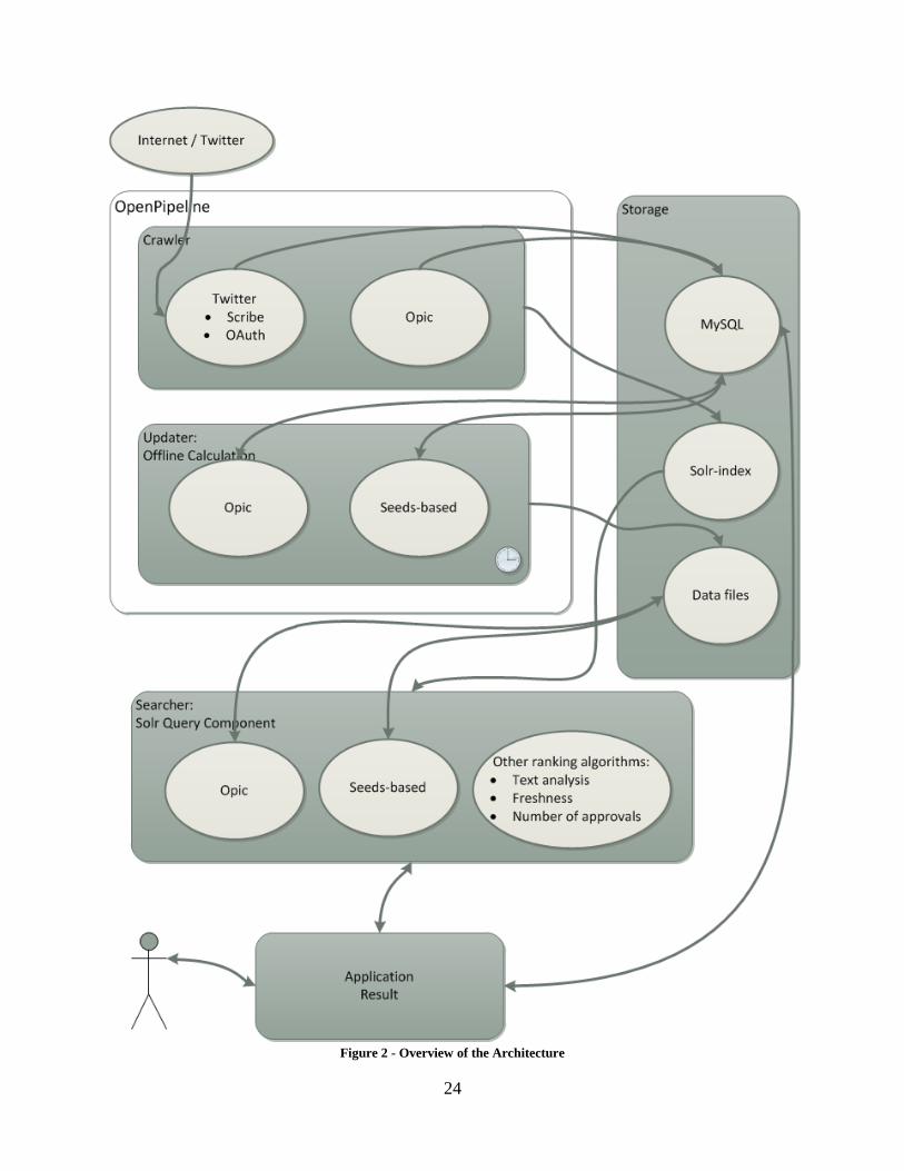
3.3 System design As we can see in Figure 2, we have five major components in our system: a crawler, a scheduled

updating process, a few storage systems, a search handler and a web application.

The crawler is using OpenPipeline to gather and process the data from Twitter and submit it to

the Solr index. The crawler uses Adaptive OPIC and updates user information which is stored in

a MySQL database. The updater process is also implemented as a job in OpenPipeline in order to

make it run regularly and on a schedule, in our implementation once every sixth hour. This could

also be done as a job using the Unix-command Cron, but with OpenPipeline we got easier

monitoring and configuration. The updater calculates the data needed to estimate the relationship

distances between the users that are saved in the database, and saves it to a data file; it also saves

the current OPIC score from the database to the same file.

The searcher is implemented using Solr as a custom request handler. The searcher uses the data

from the Solr-index and the data files in order to fetch and sort the result with our ranking

algorithms, when receiving a query.

Finally there is the application linking it all together; it submits the search queries from the user

to Solr and presents the resulting documents in a human readable format. It uses the database to

23

store our registered users for whom personalized searching is possible, so that the crawler can be

made to immediately fetch the connected social media accounts. While searching, the application

can also set up customized weighting on the ranking algorithms that will be used on the results.

24

Figure 2 - Overview of the Architecture

25

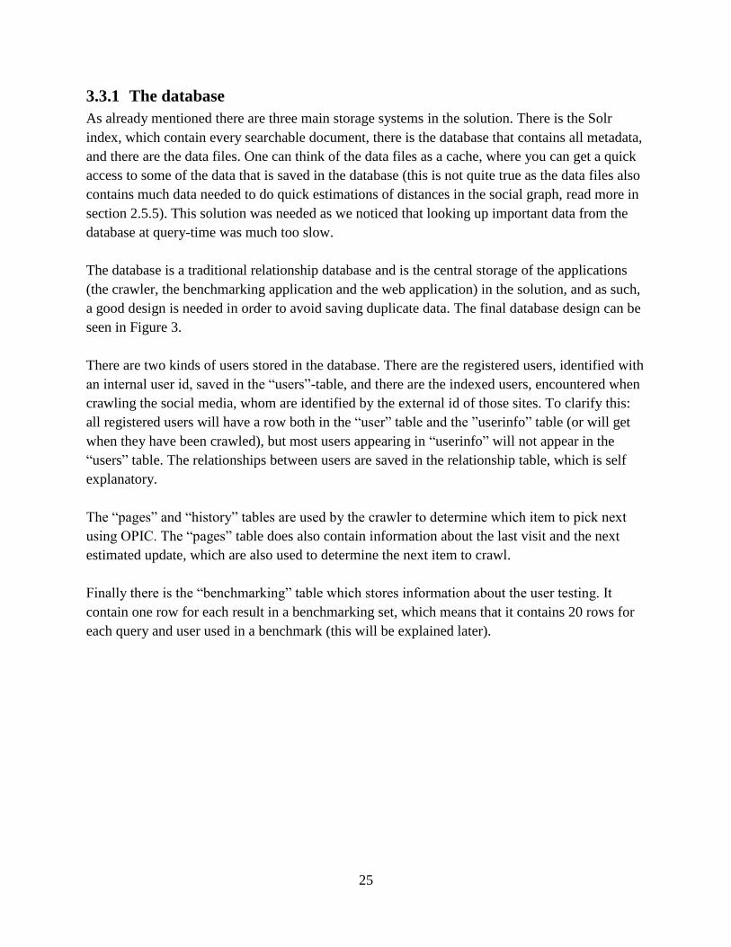
3.3.1 The database

As already mentioned there are three main storage systems in the solution. There is the Solr

index, which contain every searchable document, there is the database that contains all metadata,

and there are the data files. One can think of the data files as a cache, where you can get a quick

access to some of the data that is saved in the database (this is not quite true as the data files also

contains much data needed to do quick estimations of distances in the social graph, read more in

section 2.5.5). This solution was needed as we noticed that looking up important data from the

database at query-time was much too slow.

The database is a traditional relationship database and is the central storage of the applications

(the crawler, the benchmarking application and the web application) in the solution, and as such,

a good design is needed in order to avoid saving duplicate data. The final database design can be

seen in Figure 3.

There are two kinds of users stored in the database. There are the registered users, identified with

an internal user id, saved in the “users”-table, and there are the indexed users, encountered when

crawling the social media, whom are identified by the external id of those sites. To clarify this:

all registered users will have a row both in the “user” table and the ”userinfo” table (or will get

when they have been crawled), but most users appearing in “userinfo” will not appear in the

“users” table. The relationships between users are saved in the relationship table, which is self

explanatory.

The “pages” and “history” tables are used by the crawler to determine which item to pick next

using OPIC. The “pages” table does also contain information about the last visit and the next

estimated update, which are also used to determine the next item to crawl.

Finally there is the “benchmarking” table which stores information about the user testing. It

contain one row for each result in a benchmarking set, which means that it contains 20 rows for

each query and user used in a benchmark (this will be explained later).

26

Figure 3 - The database design

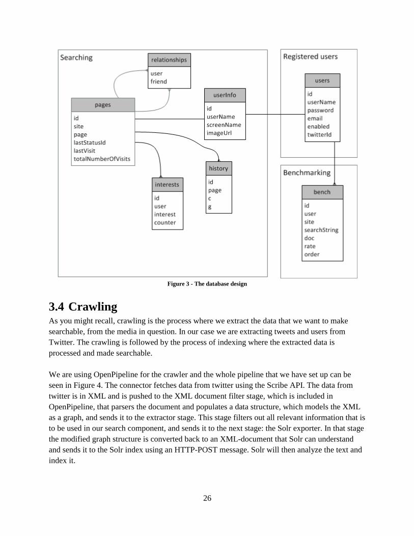
3.4 Crawling As you might recall, crawling is the process where we extract the data that we want to make

searchable, from the media in question. In our case we are extracting tweets and users from

Twitter. The crawling is followed by the process of indexing where the extracted data is

processed and made searchable.

We are using OpenPipeline for the crawler and the whole pipeline that we have set up can be

seen in Figure 4. The connector fetches data from twitter using the Scribe API. The data from

twitter is in XML and is pushed to the XML document filter stage, which is included in

OpenPipeline, that parsers the document and populates a data structure, which models the XML

as a graph, and sends it to the extractor stage. This stage filters out all relevant information that is

to be used in our search component, and sends it to the next stage: the Solr exporter. In that stage

the modified graph structure is converted back to an XML-document that Solr can understand

and sends it to the Solr index using an HTTP-POST message. Solr will then analyze the text and

index it.

27

Figure 4 - The crawling pipeline

3.4.1 OPIC implementation

So far we’ve been a bit vague when it comes to what the connector actually fetches from Twitter

and in what order. To understand this one must first consider the conditions that we are working

under. The APIs of the social media sites all have different kinds of limitations on how much

data an application can access. For example Twitter currently allows 350 accesses to their restful

API per hour by default (read more in section 2.3.2). Although the exact number of requests

possible isn’t important, we need to create a crawler that makes the number of requests allowed

count. To crawl a user and his or her latest statuses we need two requests, one to fetch the users

that he or she is following, and one to fetch the latest statuses written by that user.

We want to obtain as important data as possible with the limited number of requests available.

To achieve this we need to use some kind of measure on which statuses we need to get next.

Adaptive OPIC is an algorithm that does this for us, although it isn’t designed for use on social

media statuses, but for web pages in general. The problem is, in other words, that we cannot

model statuses as a graph, since they do not possess any natural relationship with each others.

However, as we are considering the users to be nodes in a graph, we can in fact think of a social

network as an alternative to the web. As the users are the authors of the statuses, whenever a user

is visited, the latest statuses that has been written by him or her is fetched.

To summarize this, our basic idea was to use OPIC, where we model each social network user as

a vertice, and let the outgoing edges be connected to those users that he or she is following. With

this we can always have a good estimation of which of all users that we have encountered are

currently considered the most important one. With this notion of important we are referring to a

Pagerank-like attribute and mean the user with the most important followers (read more about

Pagerank in section 2.5.1).

OPIC is implemented in the connector stage. Some technical details are written here, read about

how the algorithm works in section 2.5.2.

28

We use variable window of size 4, as this yields the best results in the experiments done in [11].

The cash is stored in memory and the cash history is stored in our database. This means that the

OPIC-algorithm only need to do one database access each time a page is visited.

3.4.2 Crawling policies

The selection policy is a combination of a few factors. There is the current cash of a page

according to the OPIC definition. There is the estimated next update of a user, i.e. the next time

we think that the user will post a new status. And finally there are the registered users that are

prioritized. How these factors are used to determine what user to fetch next will be described

now.

First the program check if there are users that exists in the “users” table in that database that

doesn’t exists in the “userinfo” table. That means a registered user, who should be able to get

personalized ranking should be crawled as quickly as possible and are always done first.

Secondly we get the top users in the “pages” table in the database with the highest current cash.

Those users are iterated over, and the first user with an estimated next update time higher than

the current time, is picked. That is, of the more important users the first encountered one that we

think has done an update since the last time he or she was crawled will be picked.

Our politeness policy is designed to spread out our allowed requests to Twitter evenly during an

hour. If the crawler detects that the limit of requests allowed are decreasing it will gracefully

increase the time between our requests.

3.4.3 Extracting data

We have already mentioned that the extractor stage is filtering out the information that is to be

saved from the Twitter data. It will also format some of that information to something that will

be easier or faster to use later on. Timestamps received from Twitter are for example formatted

in a way that is easy for humans to read, but in order to do quick calculations of how old a status

is (more on freshness ranking later) we convert it to a Unix-timestamp, which is simply the

number of seconds since the first of January 1970. By doing this, the quite expensive operation

of converting a human readable date into a simpler format is only done once per status. And

calculating how old a status is reduced to a quick arithmetic operation at query time.

The extractor stage is also responsible for saving data about the user into the “userinfo” table in

the database and to download the users profile image. The relationships are also stored in the

database, but they are updated from the connector at the same time that the relationships are

handled by OPIC.

29

3.5 Searching Searching is the key component in our solution. We need a search solution that is fast and precise

even if the dataset searched is big. For that we are using Apache Solr. We have learned that Solr

is a very competent tool, and is very fast. Because of this we wanted to use the original

functionality of Solr and wanted to modify it as little as possible.

We did however ran into some problems when we tried to make it run a customized ranking

algorithm. But Solr is very flexible and is based on components and plugins, which are all easy

to customize and to swap. Read more on how the ranking system is implemented later.

3.5.1 The schema

The schema is the definition of what is stored in the Solr-index. Think of it as the header of a

table. The schema that we are using contains the following fields:

Id

CreatedAt

Text

UserId

UserScreenName

UserName

NrApprovals

ReplyTo

Site.

The id is the same id as is used by twitter, and it’s also used by Solr (i.e. it is defined as the

unique field in the schema). If more social media sites are added, a prefix should be applied

before the id to keep the ids unique. CreatedAt is the time when the tweet was posted formatted

as a Unix-timestamp. The userId is the id used by Twitter, we do store more information about

the user in our own database, and this id is used to quickly find that information. The

userScreenName and userName is the real name and the twitter name of the user. The screen

name is the name that is mainly used to identify a user on Twitter and is unique. The

nrApprovals field is the number of retweets that has been done on a specific tweet. This can also

be used on other social media, and be used to count the number of “likes” a status has on

Facebook for instance. Site is used to keep track of where the current document comes from. As

only Twitter is used this is currently always Twitter, but will be useful if more social media sites

will be indexed in the future.

The main field in the schema is the text field. It’s in that field that the search occurs. The text is

tokenized on white spaces and word delimiters. It’s filtered to lower case, stop words (“the”,

”of”, etc.) are removed, and the text is finally stemmed to its original form. We are using an

30

english stemming algorithm and an english stop filter dictionary as english is the most common

language of Twitter.

Notice that both indexed documents and search queries needs to be tokenized in the same way in

order to make searching work.

3.5.2 Configurations

For the search engine we are using the OR-operator and on the benchmarking system we are

using the AND-operator.

Using the OR-operator will make sure that the result from the searches will be complete. This

together with a good ranking algorithm will guarantee that the user gets a result which is both

complete, and in a good order.

We did also define a custom request handler, “smsearch”. A request handler defines what

happens when a request is submitted to Solr, or more specifically which components that are

activated and in which order [21]. The important difference with our request handler compared

to the default one, are that we have a custom search component that handles our customized

ranking, but more on that later.

3.6 Ranking for social networks For common web pages the amount of links to a page works as a very good measurement of

quality for that web page, but there does not exists anything that intuitively corresponds to links

for social media statuses. And as far as we know there are not any publically available ranking

algorithm design specifically for social media statuses (the social media sites probably have their

own, but they are kept secret), so we have to come up with one ourselves.

Intuitively there are a number of parameters that can be used to determine the quality or

relevance for a status. If we categorize these parameters we find out that they can be divided into

three groups: general, social media specific and personal parameters. Social media is about social

experiences, so we think that the result of a search should be as personalized as possible. We

give an overview of the parameters we think are the most important here, and explain and

motivate them, as well as discuss how they are implemented, later in this section.

General parameters

Text analysis

Freshness

31

Social media parameters

Approvals

Popularity

Personalized parameters

Distance in the social graph

Personal interests

Location

In [8] they come to a similar conclusion but divides it in three different categories for measuring

friendship strength (i.e. user to user ranking). They replace our personalized category with the

categories social and spiritual ranking and keep the general ranking category. They define social

ranking as relationships, e.g. minimum distance in the social graph, and spiritual ranking as the

similarity between users, e.g. users that normally likes the same things, but are not necessarily

close in a social graph.

3.6.1 The ranking parameters

Of the parameters that we suggested in the last section we have implemented all but one. These

are described here. The location parameter is left for future work to investigate.

3.6.1.1 Text analysis

Motivation: It’s obvious that the returned results of a query should have something to do with the

query, but you can make it more cleverly by analyzing the text to determine how much the result

has to do with the query.

Implementation: TF-IDF is the basis for the ranking done by Lucene. We are simply reusing that.

3.6.1.2 Freshness

Motivation: Freshness is categorized as a general parameter, but we think it especially important

in social media where everything happens very fast. In Twitter, for example, you can see the

current trending topics, and they are changing several times every day. We think that the later the

status was written the more important it should be. It also makes sense if the user is searching for

a recurring event (such as a championship in some sport), then he or she would probably want to

know about the latest time the event occurred.

Implementation: We define freshness as the inverse of the amount of time (in seconds) from now

to when the entry was written. In order to optimize the calculations, the time is at crawl-time

converted from Twitters human readable format to a standard Unix timestamp which all query-

time calculations are done on.

32

In this equation x is the status that is to be ranked, t is the current timestamp, and tx is the timestamp of

the x.

3.6.1.3 Approvals

Motivation: Many social media provide the ability for a user to approve of what is written in a

status. In Twitter this is done by retweeting it. If many users likes a status then a querying user is

obviously more likely to find it useful too.

Implementation: Simply implemented as a number of how many users that has approved the

document, the higher the better. Currently Twitter stops counting at 100 retweets and mark any

number above that limit with 100+, which we store as 101. That means that the number of

approvals currently will be between 0 and 101 in our implementation.

3.6.1.4 Popularity

Motivation: The OPIC rank is basically an estimation of the Pagerank algorithm, with the only

difference that the rank can be calculated at any time instead of off-line as is done by the original

Pagerank.

Implementation: The data needed to calculate the OPIC-rank is done at crawl time, and the actual

rank is straight-forward to implement. Although the data needed to calculate the current OPIC-

rank is stored in the database, and database connections are slow. As we did not want to do a

database query for each unique user at query-time we had to find another solution. First we tried

to submit the current rank to the Solr-index at crawl time. This was a failure however as the

average OPIC-rank are decreasing as the index grows (the OPIC-rank is a relative and not an

absolute measure), and in our implementation we would only update the rank as we recrawled

users. The result was that users that were crawled a long time ago would generally have a much

higher rank than newer users. We solved this by letting the OPIC-rank be calculated in our

scheduled updater program and then stored in the data file, so that only a look-up in that file

would be needed at query time. This solution is efficient and accurate, although maybe not

completely up to date as the updater program only runs at specified intervals.

3.6.1.5 Estimated relationship distance

Motivation: How close is the author of a status to you in the social graph? What a friend of a

friend has to say is generally more interesting to you then what a total stranger would have to

say. Closeness in a social graph can also imply a physical closeness in the real world. This means

that what statuses concerning things that happen in the same town as you live might indirectly

affect the ranking of those documents positively.

33

Implementation: The data needed to do an actual estimation of the distance is done in the

scheduled updater program. The updater program first builds the whole graph from the

“userinfo” and “relationship” tables, which is kept up to date by the crawler. Then it selects, at

random, 10 % of the nodes to be landmarks and from all these nodes a breadth-first search is

done and the distances from all nodes to all landmarks are saved to a file. This file is then used

on query time, so we only have to read the affected rows from the file, and calculate the distance

as described in the background chapter.

3.6.1.6 Interests

Motivation: As already mentioned you are mostly not that interested in what a total stranger has

to say, unless of course that stranger shares some interests with you. If a status is concerning a

topic which you have written about yourself, then it will probably be much more interesting to

you.

Implementation: In our implementation, we are using the hashtags a user have used in his or hers

statuses. We are extracting the top five most used tags in the “Twitter extractor” stage in the

pipeline of the crawler and save the tags and the number of occurrences, appearing in the latest

crawled statuses, in the “tag” table in the database. Then in query time these five tags is used to

make a new search in the index, with those tags and the original search term as parameters, and

the Lucene scoring of this result is then used to contribute to the total ranking score.

3.6.1.7 Location

Motivation: A new feature of social media is the ability to add the authors physical location to a

status. How close to where yourself are at the moment was a document in the result written? The

closer it is, the more interesting it will probably be.

Implementation: Not implemented, read about it in the section 4.5.

Note that the ranking returned by all individual ranking algorithms will be normalized to a value

between 0 and 1. Read more about that later.

3.6.2 Proposed improvement of Seeds-based algorithm

While discussing how the seeds-based algorithm worked, we came up with an alternate version

of the algorithm in which you sacrifice a little precision for speed and reduced storage

requirements.

Instead of saving all distances to all seeds from every common node, we only save the distance

to the one seed that is closest, and for every seeds we save the distances to every other seeds.

Then when we want to calculate the distance between two nodes we read what seed is nearest

them, and take the distance between them.

34

Example:

We use the same graph as in the previous example (Figure 1).

We still have B, C and D as landmarks, but we only save the distance to the seed which is

nearest, and all distances between the seeds.

Node B C D

A 1 - -

B 0 1 2

C 1 0 2

D 2 2 0

E - - 1

To calculate the minimum distance we now just add the two nearest seeds, plus the distance

between these seeds (A → B → D → E): 1 + 2 + 1 = 4.

3.7 The ranking system In the last section, the implementation of each ranking parameter was discussed, in this section

we will focus on how everything is fitted together to merge the ranking algorithms together into

a single ranking parameter that can be used to sort the results on. We will also discuss some

more technical implementation details with the use of Solr in mind.

3.7.1 Solr ranking

As default Solr provides a good relevance model, based upon TF-IDF out of the box. This is

highly customizable and you can simply boost different phrases or fields, either at crawl-time or

at query-time [21]. Personalized ranking, for example, can be done by boosting a certain phrase

that the current user is known to like.

Furthermore there is a system called functional queries that are provided to extend this further

[21]. Using this one could create a customized ranking by combining functions which are

defined in Solr. For example boost newer documents by calculating the time that has passed from

now to when the document was written, simply by adding a function call directly from the query.

As powerful and as flexible this is, we felt that it wasn’t quite enough for what we wanted to do.

Regardless of you look at it, the supplied Lucene score would always be the basis for the

35

ranking. But we only wanted that the Lucene score should be a part of the ranking, treated

equally to the other ranking algorithms we were designing.

And in order to add things like the minimum distance from the querying user to each author of

the documents in the results, we had to add those fields to the results directly at query time. And

that is something that we don’t think is possible with the current version of Solr using the

supplied ranking algorithms.

3.7.2 Our ranking model

We define the ranking of a status, x, like this:

Where u is the user performing the query, Q is the set of all words in the query. R is the set of

ranking methods implemented (in this formal model you can think of them as lambda-functions

stored in a vector, though the real implementation is different) and w is the set of weights for

each ranking algorithm. Also note that each is supposed to be normalized and return values

within the following interval.

Therefore the actual rank for a status, x, will be between 0 and the sum of all weights, w.

3.7.3 Efficient ranking

A big part of our ranking calculations occurs at query time. This means that when the user hit

”search” the ranking of each individual status in the result are ranked at that very moment. This

makes it very important to make the ranking as efficient as possible.

The key is to make these calculations as light and fast as possible. A look up in a table is, for

example, almost always faster than performing an actual calculation. Therefore we try to do the

more expensive calculations off-line in our updater program instead of at query time.

This is what happens at query time: The query is sent into Solr and Lucene which returns a set of

document combined with a score calculated by Lucene, which is mainly based upon text-

analysis. This set of documents and the Lucene score is sent to our ranking class. The ranking

module takes the set of documents and creates a new rank for each document based upon our

different ranking algorithms (where the Lucene ranking is one). As already noted each ranking

algorithm is normalized and can be weighted for a customized ranking.

36

3.7.3.1 Off-line calculations

We got this idea to use a separate and independent process for the more expensive calculations,

so that we would only have to do look ups and as few calculations as possible at query time.

Of course it is not quite that simple, you can’t simply do all possible calculations for all users

and store them in a file somewhere as the storage needed for that would be way too big.

There are two kinds of data that are calculated. There are the kind of data that is completed and

ready to use directly (i.e. the OPIC rank), and there is the kind of data that would require

additional computations (i.e. the Seeds-based ranking). In the case that requires additional

calculations this works very well as you can pre-compute data that is shared for many users.

This could maybe also be done as a part of the crawling, but since those calculations really is of a

separate kind from the processing done in the crawler, we felt that it would be better to use it as a

separate scheduled process that runs at some predefined recurring intervals.

3.7.4 Implementation details

In order to meet the requirements that we had set for our relevance model, we had to implement

a custom search component for Solr. To do this we used Java and extended the

QueryComponent-class.

The overridden process function in that class makes the search based upon the submitted query

parameters. The document list, matching the query, is then processed. The original Lucene score

is preserved, and the document list is then submitted to our ranking class.

The ranking class iterates over the ranking algorithms, calculating the scores, normalizing and

weighting them as described earlier. The ranking scores are then added as a new field to each

document and returned to the process function again.

The search component orders the list by this new field, collects some statistics about the time

different steps took to do (for evaluation and debugging purposes), adds some metadata (such as

the query time and the total number of documents returned) to the result, and sends the response

on to the next step in the request handler.

3.8 The user application The focus on this project was really not on the end user experience. But since Solr only returns

the results formatted in XML and since asking a good query might be a little technical we felt

that a simple user application would be needed.

37

A simple web application was written in PHP. The application mainly creates a query based

upon input from the user and sends it to the Solr server. The returned XML from Solr is parsed

and is presented to the user in formatted HTML that can be viewed using a web browser.

In the result section you can get a feel for how this application looks like and how it works from

a users point of view.

3.9 Benchmarking We think that benchmarking ranking results from social media should be subjective and based

upon opinions of social media users rather than some mathematical models. In [8] they use real

persons active in a social community to measure the effectiveness of their ranking methods, and

that is something we wanted to do as well.

The testers that we recruited were told to register in our benchmarking web application. There

they provided their Twitter user name. Their Twitter account was then instantly crawled. After a

few days, when we made sure that the user and some of the people he or she was following had

indeed been indexed, we asked the tester do the benchmarking test.

The test was done in this way: The user performed a number of arbitrary queries of his or her

choice to the search engine. We asked the user to do a query that was as specific as possible, and

preferably a query that would be interesting to the user. There were no limitations on what query

the user could choose, but the amount of returned results had to be in a certain interval (at least

30 results and as most 250 results).

Apart from the requests that the query should be specific and interesting no attempts was made to

control what the users would search for. We discussed among ourselves whether we should make

the user search for queries that would be adapted to suit the different ranking algorithms (like

asking the user to make one search for a recurrent event for example), but we felt that the queries

should be something that the test subjects would actually use on real search engine.

Now, from the search result the application would randomly choose a number of documents, in

our case 20. The documents were shuffled and presented to the user one by one. The user would

then grade the document on a scale from one to five on the basis of how relevant the document

was to the query.

The benchmarking system is implemented as a simple web application written in PHP. In Figure

5 there is a screenshot of what the application looks like. The application is written in swedish as

all our test subjects was having swedish as their primary language and we simply felt that it

would be better to use swedish than english. On the top left you have a list of all the documents

38

that is to be graded and the grades of those you are done with. In the middle is the current tweet

that you are currently grading; in the bottom are the options of how you can grade it.

Figure 5 - The benchmarking application

The results are selected using the AND-operator when we randomize the documents to

benchmark on. We think that the benchmarking will be more accurate if we make the user

choose as specific queries as possible, i.e. queries with multiple terms. Using the OR-operator on

the result might present many results that are just too random. Note however that when we

compare the ranking the results ranked by the actual search engine is fetched using the OR-

operator as usual (not that it would make any difference).

Of course it would be ideal if we could have the testers benchmark every item in a result instead

of just a few randomly selected documents, but as the results could be very big this could be very

annoying for the users. We compromised by limiting the results by using the AND-operator and

making sure that a test result (before the documents to test on were chosen) contained a number

of results within a specific interval.

We compare the results of all benchmarking tests with our relevance system using NDCG. We

do some iterations trying out different weights etc.

After the test was done we calculated the NDCG value for three different (0, 0.5 and 1) weight

value on five different algorithms (text analytic, popularity, combined freshness and approvals,

relationship distance and interests, that is a total of 35=243 values per test). We took the averages

of all the tests and generated the table in Figure 13 in the result section.

3.9.1 Performance testing

We needed to make sure that the queries were executed fast in order to make sure that the

ranking algorithms actually would work for real. The testing is done using a number of synthetic

queries containing different number of keywords appearing with different frequencies in the

indexed data. The queries are executed after each other using a simple script, each query with a

user attached in order to get personalized ranking.

39

We have performed the tests using Ubuntu Linux on a laptop with an Intel i3 processor and a

memory size of 4GB and we were running Solr 1.4 on a Tomcat server.

40

4 Results We will now describe what our final proof of concept search engine looks like. How the test

results came out and how well the solution works when it comes to performance and precision

will also be described. We will finally discuss possible applications and extensions of the project.

4.1 The search engine We will start the result section by showcasing the concept search engine that we have created for

social networks, and what it looks like from a user’s point of view.

Although we haven’t focused on the user interface, we wanted to create something that we could

use to demonstrate our concept search engine. The user interface makes the query-syntax to Solr,

and the XML-response from Solr invisible to the user.

We believe that user interface of a search engine should be as simple as possible. On our concept

we emphasize this by making the text field and the search button by making them big and

placing them in the center, as can be seen in Figure 6.

Figure 6 - Screenshot from the search application #1

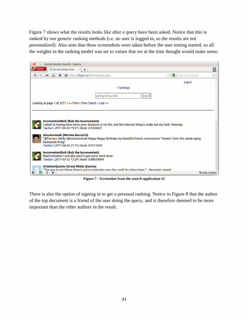
41

Figure 7 shows what the results looks like after a query have been asked. Notice that this is

ranked by our generic ranking methods (i.e. no user is logged in, so the results are not

personalized). Also note that these screenshots were taken before the user testing started, so all

the weights in the ranking model was set to values that we at the time thought would make sense.

Figure 7 - Screenshot from the search application #2

There is also the option of signing in to get a personal ranking. Notice in Figure 8 that the author

of the top document is a friend of the user doing the query, and is therefore deemed to be more

important than the other authors in the result.

42

Figure 8 - Screenshot from the search application #3

Finally there is an expandable section of settings where the user can adjust the weights of the

different ranking algorithms. This is used for testing and demonstration purposes. Notice how in

Figure 9 the weight of the Lucene score is increased very much, and a document that just

contains the phrases in the query (it’s ranked higher than the others because the term “do”

appears two times, but in different forms) is returned. That document belongs to a user that just

collects quotes and would maybe not be that interesting for the user.

43

Figure 9 - Screenshot from the search application #4

4.2 Experiments The experiments done can be categorized into two categories. There is the performance based

testing and there is the more subjective user testing. The outcome of these tests will be described

here.

4.2.1 Sample data

The final sample data that we has acquired during the project has around 5000 indexed users,

750 000 indexed tweets, and 2 500 000 registered relationships. We think that this is a quite big

index, at least big enough to test our application in a good way. Although the amount of tweets

indexed is not even a hundredth of what Twitter produces daily [3].

4.2.2 Performance testing

How long time our different ranking algorithms take to execute has been measured. That is, the

time taken to execute an algorithm at query-time in milliseconds as a function of the number of

documents in the result. Some of the algorithms are, as already discussed, partly or completely

pre-calculated, either at index time or in a scheduled updater program. We haven’t measured the

time these off-line calculations takes to do, because we do not think that those measurements are

very important, and we are prioritizing keeping the time for processing queries low. Because of

44

this the implementations of the off-line calculations are not as optimized as they could have

been.

You should note a few things with these results. First, the time of calculating the Lucene score is

not included. As this is implemented in Lucene it’s out of our control to measure. Secondly, the

total ranking time is how long time our ranking component takes to execute. It’s the sum of the

time that the different algorithm takes to execute, but with some additional overhead of

generating user lists from the documents and similar tasks. Also notice that Solr and Lucene

takes some time when doing the actual search and calculating the Lucene score, and this is not

included in the total time here. We do know however that both the searching and Lucene score

is calculated quite fast as they are basically just table look ups in the index. Finally remember

that the Seeds-based and interest-based algorithms are personalized ranking algorithms that will

not be included in a generic (non-personalized) ranking.

Figure 10 is a chart showing the result of all algorithms plotted together. As can be seen the

Seeds-based distance estimation-algorithm is the slowest one. This is expected, because although

many calculations are done off-line, some calculations need to be done at query time [14]. And if

we consider that calculating distance between nodes in a graph normally is very computationally

expensive, we think that it’s quite impressive to do a pretty accurate estimation of the distance

from the user searching to about five thousands other users in just above five seconds. Note also

that we are using our Seeds-based algorithm with our proposed improvement here.

Figure 10 - Comparison of ranking algorithms

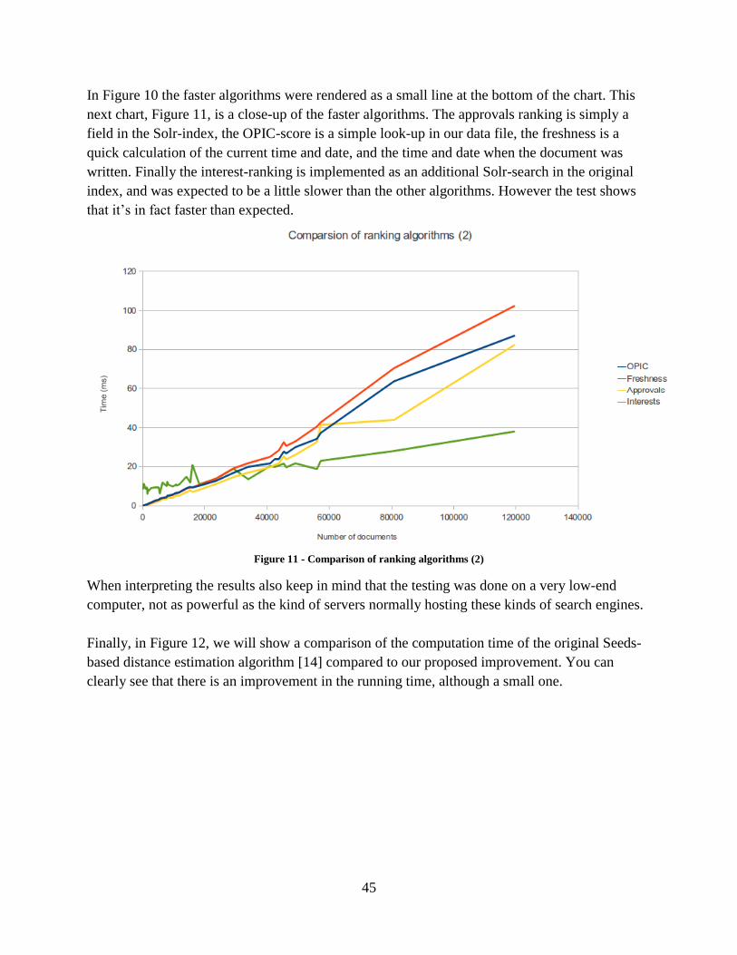
45

In Figure 10 the faster algorithms were rendered as a small line at the bottom of the chart. This

next chart, Figure 11, is a close-up of the faster algorithms. The approvals ranking is simply a

field in the Solr-index, the OPIC-score is a simple look-up in our data file, the freshness is a

quick calculation of the current time and date, and the time and date when the document was

written. Finally the interest-ranking is implemented as an additional Solr-search in the original

index, and was expected to be a little slower than the other algorithms. However the test shows

that it’s in fact faster than expected.

Figure 11 - Comparison of ranking algorithms (2)

When interpreting the results also keep in mind that the testing was done on a very low-end

computer, not as powerful as the kind of servers normally hosting these kinds of search engines.

Finally, in Figure 12, we will show a comparison of the computation time of the original Seeds-

based distance estimation algorithm [14] compared to our proposed improvement. You can

clearly see that there is an improvement in the running time, although a small one.

46

Figure 12 - Comparison of distance estimation algorithms

4.2.3 User testing

The user testing was carried out by six users that ran a total of 28 queries, each user doing

between 3 and 8 queries. Most queries were concerning special interests the test subjects have,

such as musical artists, movies or sport teams. Some queries were for celebrities, and some

concerned certain products, different kinds of cell phones seem to have been a popular topic. In

some cases several users was searching for the same phrase, and in at least one of those cases we

think that the users was searching for different things but with the same name. To protect the

integrity of our test subjects, we will not go into any more details about the queries asked.

In Figure 13 you can see the average NDCG values from all the tests with the different weight

values. The original Seeds-based algorithm is used to estimate a rank based on relationship

distances. Where the different weight values are as follows:

a) Text analysis

b) Popularity, i.e. OPIC weight

c) Combined weight for freshness and approvals

d) Estimated relationship distance

e) Interests

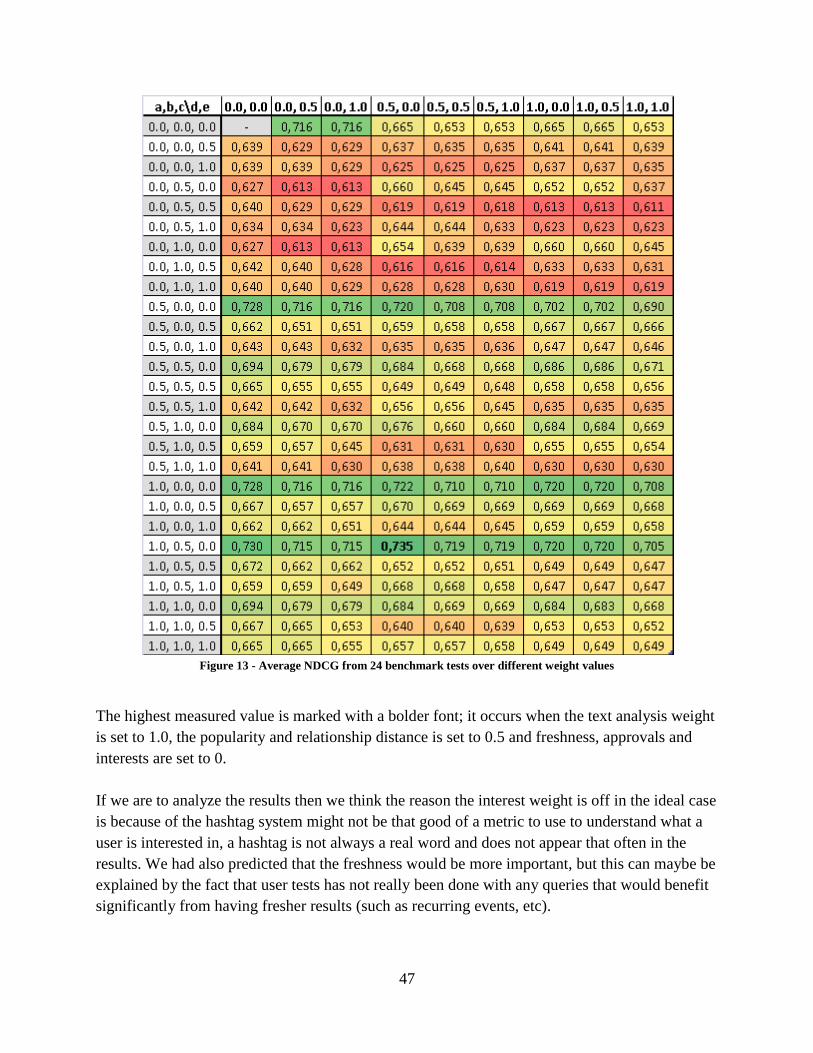
47

Figure 13 - Average NDCG from 24 benchmark tests over different weight values

The highest measured value is marked with a bolder font; it occurs when the text analysis weight

is set to 1.0, the popularity and relationship distance is set to 0.5 and freshness, approvals and

interests are set to 0.

If we are to analyze the results then we think the reason the interest weight is off in the ideal case

is because of the hashtag system might not be that good of a metric to use to understand what a

user is interested in, a hashtag is not always a real word and does not appear that often in the

results. We had also predicted that the freshness would be more important, but this can maybe be

explained by the fact that user tests has not really been done with any queries that would benefit

significantly from having fresher results (such as recurring events, etc).

48

This highest average NDCG value is 0.735 and if we look at the base case (where we would only

use the Lucene provided score as is the default ranking in Solr) which is 0.728, we have gained a

slight improvement.

We didn’t expect any values to be very much higher than the base case as it rarely is in these

kinds of tests in information retrieval. And as they argue in [8] even a small improvement in

information retrieval is statistically significant.

Also note that because of limited amount of space in the table we have increased the weights

with very coarse steps. This resulted in a test with all weights tested but with only a few values

tested on each weight. The accuracy could be increased with a test where more fine-grained steps

are used, and possibly with some clever machine learning algorithms applied to find out the

optimal weights, but that is left for future work.

4.2.4 Testing of the alternative version of the Seeds-based algorithm

To test our proposed improved seed based algorithm we calculated the distance from one node to

eight hundred other in our sample data with both the Seeds-based algorithm and the proposed.

Then we did the same test but with the breadth-first algorithm to get the actual distances. We

calculated how many steps off from the real value the different algorithms had estimated the

distance to, and from that took the amount of distances that was less than 10 steps from the real

distance.

This result from these tests is that 50 % of the results from the original Seeds-based algorithm

were less than 10 steps away from the real distance and in our proposed version of the Seeds-

based algorithm the same amount were 30 %.

The tests were conducted with the settings to use 10 % seeds for booth algorithms. This

generated a file of about 7 MB for the original Seeds-based algorithm and a file of 0.8 MB for

our proposed version.

So to conclude the results of the testing of the proposed improved seeds based algorithm is that

the accuracy is worse than the original algorithm. But the benefits of this algorithm are that the

file size of the pre-calculated distances is much smaller than the original algorithm and the online

calculations takes a little less time than in the original algorithm as stated in the performance

testing section earlier.

49

4.3 Discussion During the project there are a few things that we have learned and that we want to highlight.

4.3.1 You can’t index everything

While this statement might not be true for all social media services (a small corporate social

media on Yammer for example might be completely indexable), it’s something that almost

always will apply when it comes to social networks. The solution is however quite straight-

forward: know what you want. When creating a search solution you must know what kind of

data that should be index, and then apply some clever method to get just that. This problem isn’t

really something new, the same applies for all search engines that indexes the web, and there

aren’t any search engine that can guarantee to find everything on the web. Although there is an

important difference here. When it comes to social media the difference is that the limitations

might lie in the number of requests that can be sent the API and the hardware of where the

solution is running.

We deal with this problem by doing a focused crawling on the importance metric of an

individual user, by the number of followers he or she has, and the importance of those followers,

with some small additions (read more in section 3.4). We think this works well but that this can

be taken even further (read more in section 4.5).

4.3.2 Old relevance models are still useful

We have found out from our results that the old and tested models that has been used to measure

relevance on other sources (such as the web), are still good and useful in this context. Pagerank,

text analysis by TF-IDF and freshness are all good ways to measure relevance. Our user testing

shows that the TF-IDF ranking provided by Lucene is especially good here.

4.3.3 Personalized ranking

Social networks are really about what happens around you, what your friends are up to. We

suspected that a personalized ranking was an important element, and the user testing shows us

that we were right about that. And though the distance in a graph turned out to be more important

than the interest based ranking we still think that both these methods of ranking are useful,

although just as how useful one methods is over the other may be dependent on the context,

implementation, and what the user is looking for.

4.3.4 Efficient solutions with personalized ranking is possible

There are several ways to do personalized ranking. The more efficient way is by simply boosting

certain categories or phrases based upon the interests of the user searching. But doing

personalized ranking with the distance in the social graph between users instead is even better. In

order to do that one has to be clever. We don’t think there exist a good way of doing this with the

50

exact distance, but our user testing shows that calculating estimations of the distance is good

enough. And our performance testing shows that this can be done quite efficient. Usage of

offline calculations as much as possible is however a requirement.

4.4 Applications for search in social networks So, as we got a concept search engine for social networks, the question to ask is, what now? How

can this be used? We discuss some examples of what we think would be the main uses of this

kind of search application, but the possibilities are of course unlimited.

4.4.1 Personal search

We now have a search engine where you can connect your user in a social media to get the

benefit of ranking based upon your profile and your relationships, but this is currently limited to

searching in social media. We think that personal ranking using data from a users profile in a

social media can be applied to other kinds of search.

For example, when you analyze the profile of the user and finds out his or hers interests, you can

then use that information in ordinary web search and boost documents matching those interests.

4.4.2 One search engine, many sources

One of the goals with the project has been to make the relevance models as general as possible.

With this in mind, there should be no problems aggregating content from several social media

services into one search engine, and apply a unified relevance model to all of them.

You could also mix content from social media services with any other content, such as web

content, and make it all searchable from one single place.

4.4.3 Analyzing

If someone needs to understand what real people really thinks about something, such as a brand,

a product or an event, then microblogs, such as Twitter, would be good sources. A search engine

could quickly filter out and order what the user is looking for, and based upon the results you

could quickly get an understanding of the more common opinions of something.

4.4.4 A wall sorted on relevance

One of the features in most social media is a wall, where the statuses that your friends have

written appear. However with many friends writing content, this could quickly be very much

information, too much to read through. What if it was possible to order the unread statuses based

on a relevance model? There is nothing that says that a relevance model only could be applied on

search results, and we think that our model could be applied in different contexts as well.

51

4.5 Further development There are some ways to improve our work further. We have some ideas that we didn’t have the

time to investigate that we suggest for further development here.

4.5.1 Focused crawling

Since most social media contain very large amounts of data we suggested the use of focused

crawling to get around that. What we have implemented in our crawler is mainly to use a

common notion of popularity to get the most important users of Twitter. We also use an

estimation of the next update and let registered users get a queue over which users to crawl next.

But this can be extended further. Depending on the needs of those who implement the solution

we suggest improvements to the selection policy to get an even more focused crawling. This

assumes that those who implement the search engine know what they are looking for.

If OPIC or something similar is used, one could limit the crawl to a maximum depth from the

users that the crawl start with, in order to get away from getting the most popular users of

Twitter (like Barack Obama or Oprah Winfrey) which might be considered important to many

users but might be irrelevant for the specific search engine.

As mentioned we analyze the previous tweets of a users timeline in order to calculate the

estimated time of when he or she will write something new. In a similar way one could analyze

the content to find out what the user frequently writes about and based upon that determine how

interesting that is to the actual implementation. This can also be used to determine what language

the author is writing in (also note that you can get the language from the Twitter API although

that has to manually be set by the users and might not be very reliable).

4.5.2 Geographical search

In an age of location-aware devices such as smartphones with GPS-support, many social

networks let the user add location data to the statuses that is written. Twitter is no exception and

it would be quite simple to index the location of where a tweet was written. This could be used

either as a parameter to personalized ranking so that tweets that was written in your vicinity

would be ranked higher, or to do customized queries based on locations.

52

4.5.3 Streaming API

We have used the Restful API of Twitter. There is another API called the Streaming API that

could be used. The Streaming API does not have the same limitations as the Restful API but

provides some different limitations of its own. We think that if you want to index everything that

is written by a limited amount of users then you should use the Streaming API, but if you want to

get what is written by a broader number of users, but does not need to guarantee to get

everything they have written, then you should use the Restful API. It is possible however that

you could combine those APIs, to get an even more comprehensive coverage of Twitter.

53

5 Conclusion Social networks are a hot topic right now. Bringing order in the vast amount of information that

is generated in them is an equally hot topic. There is a lot of information produced and just

keeping up with what your friends are writing is a hard task, keeping up to date with the

coverage of some specific topic is even harder.

We think that there are different approaches to bringing order in information in social media, but

most of the solutions to these kinds of problems come down to ranking content based upon what

you, the user, would find most interesting. Then whether the application is presenting it to you as

the latest unread statuses, or presenting the content received from a search doesn’t matter,

because they can still be ordered by basically the same notion of personal relevance.

What we have looked on is just that. We have created a search engine, which uses some different

techniques to calculate a relevancy on a set of documents, based upon a specific user and a

specific search query. Some of these techniques are traditional and has been used in slightly

different contexts for a very long time (such as the Adaptive OPIC algorithm), some are brand

new from very recent research (such as the Seeds-based algorithm).

We have also created a crawler that indexes Twitter, and can be extended to index any social

media site, and fetches users and the documents they have written, in a specific order based upon

our notion of importance.

We see in the results from the testing that these algorithms used for searching are efficient and

that they can be used to improve the quality of the ordering of search results. Although the

NDCG score from the testing shows only a marginal improvement, one should keep in mind that

improvements often are smaller when it comes to tests based on the subjective opinions of users.

We think that the relevance models we have assembled are good and general and that they can be

used in similar search engines. It is important to consider however that the results of this thesis

should serve more as a guideline on what to focus on when creating a search solution rather than

a generic one-size-fits-em-all model for search in social networks. And although the model can

be extended and developed further, we are satisfied with our work, and think that we have

reached the goals we set up for the project.

54

6 References 1. Makice K. Twitter API: Up and Running: O’Reilly Media; 2009.

2. Twitter website. [Online]. Available from: http://www.twitter.com.

3. What is Twitter. [Online]. Available from: http://business.twitter.com/basics/what-is-twitter.

4. Yammer website. [Online]. Available from: https://www.yammer.com.

5. Twitter API documentation. [Online]. Available from: http://dev.twitter.com/doc.

6. OAuth website. [Online]. Available from: http://www.oauth.org.

7. Scribe java library. [Online]. Available from: https://github.com/fernandezpablo85/scribe-

java.

8. Schenkel R, et al. Social Wisdom for Search and Recommendation. Data engineering (IEEE

Computer Society). 2008; 31(2).

9. Fast Search & Transfer ASA. Book of Search. 2nd ed.; 2006.

10. Brin S, Page L. The PageRank Citation Ranking: Bringing Order to the Web; 1998.

11. Abiteboul S, Preda M, Cobena G. Adaptive On-Line Page Importance Computation. INRIA;

Xyleme SA; 2003.

12. Spärck KJ. A statistical interpretation of term specificity and its application in retrieval.

University of Cambridge; 1972.

13. Salton G, Buckley C. Term-weighting approaches in automatic text retrieval. Cornell

University; 1988.

14. Vieira MV, Fonseca BM, Damazio R, et al. Efficient Search Ranking in Social Networks.

CIKM. 07 November; p. 563-572.

15. Potamias M. Indexing distances in large graphs and applications in search tasks. National

Technical University of Athens; 2005.

16. Järvelin K, Kekäläinen J. IR evaluation methods for retrieving highly relevant documents.

University of Tampere; 2000.

17. Valizadegan H, Learning to Rank by Optimizing NDCG Measure. Michigan State

University; Advertising Sciences; Yahoo! Labs.

18. OpenPipeline website. [Online]. Available from: http://www.openpipeline.org/.

19. Solr website. [Online]. Available from: http://lucene.apache.org/solr/.

20. MySQL website. [Online]. Available from: http://www.mysql.com/.

21. David Smiley EP. Solr 1.4 Enterprise Search Server: Packt Publishing; 2009.