validation of insulated joints - chalmers publication...

Validation of insulated joints

Master’s Thesis in Solid and Fluid Mechanics

ANTON WAHNSTROM

Department of Applied MechanicsDivision of Material and Computational MechanicsCHALMERS UNIVERSITY OF TECHNOLOGYGothenburg, Sweden 2011Master’s Thesis 2011:04

MASTER’S THESIS 2011:04

Validation of insulated joints

Master’s Thesis in Solid and Fluid MechanicsANTON WAHNSTROM

Department of Applied MechanicsDivision of Material and Computational MechanicsCHALMERS UNIVERSITY OF TECHNOLOGY

Gothenburg, Sweden 2011

Validation of insulated jointsANTON WAHNSTROM

c©ANTON WAHNSTROM, 2011

Master’s Thesis 2011:04ISSN 1652-8557Department of Applied MechanicsDivision of Material and Computational MechanicsChalmers University of TechnologySE-412 96 GothenburgSwedenTelephone: + 46 (0)31-772 1000

Chalmers ReproserviceGothenburg, Sweden 2011

Validation of insulated jointsMaster’s Thesis in Solid and Fluid MechanicsANTON WAHNSTROMDepartment of Applied MechanicsDivision of Material and Computational Mechanics

Chalmers University of Technology

Abstract

In track engineering, insulated joints are widely used as a key component inthe signaling system to electrically insulate track sections and thereby locate trains.However, many problems with track deterioration and signaling malfunction are re-lated to them. In spite of this, the requirements on validation testing to assure themechanical quality of insulated joints are rather low. Trafikverket (Swedish Trans-port Administration) has a standard that specifies tension tests for insulated joints.However the related bending test is not specified, which makes comparisons betweentests cumbersome. There is therefore a need to establish a standardized bending testto compare and evaluate the quality of insulated joints. This thesis outlines such astandardized test.

Further, a crucial part in the validation is operational testing. This thesis scruti-nizes the issue of how tests should be designed to assure a high statistical confidence.

Keywords: Insulated joints, bending test

, Applied Mechanics, Master’s Thesis 2011:04 I

II , Applied Mechanics, Master’s Thesis 2011:04

Contents

Abstract I

Contents III

Preface V

1 Introduction 11.1 Background . . . . . . . . . . . . . . . . . . . . . . . . . . . . . . . . . . . 11.2 Method . . . . . . . . . . . . . . . . . . . . . . . . . . . . . . . . . . . . . 11.3 Function of an insulated joint . . . . . . . . . . . . . . . . . . . . . . . . . 11.4 Common joint damages . . . . . . . . . . . . . . . . . . . . . . . . . . . . . 11.5 Limitations . . . . . . . . . . . . . . . . . . . . . . . . . . . . . . . . . . . 3

2 Approach 42.1 Mesh influence . . . . . . . . . . . . . . . . . . . . . . . . . . . . . . . . . 42.2 Investigated parameters . . . . . . . . . . . . . . . . . . . . . . . . . . . . 8

3 Load modeling 93.1 Single and double axle bogies . . . . . . . . . . . . . . . . . . . . . . . . . 93.2 Dynamic load effects . . . . . . . . . . . . . . . . . . . . . . . . . . . . . . 123.3 Rail profile . . . . . . . . . . . . . . . . . . . . . . . . . . . . . . . . . . . . 123.4 Joint position . . . . . . . . . . . . . . . . . . . . . . . . . . . . . . . . . . 123.5 Insulation material . . . . . . . . . . . . . . . . . . . . . . . . . . . . . . . 133.6 Test specimen . . . . . . . . . . . . . . . . . . . . . . . . . . . . . . . . . . 133.7 Error margins . . . . . . . . . . . . . . . . . . . . . . . . . . . . . . . . . . 14

4 Test setup 164.1 Test procedure . . . . . . . . . . . . . . . . . . . . . . . . . . . . . . . . . 16

5 Evaluation of field validation tests 215.1 Determining which joint type that has the highest quality . . . . . . . . . . 215.2 Quality factor comparison . . . . . . . . . . . . . . . . . . . . . . . . . . . 235.3 Mean life estimation . . . . . . . . . . . . . . . . . . . . . . . . . . . . . . 25

5.3.1 Mean life time estimation, five joints of each type . . . . . . . . . . 265.3.2 Mean life time estimation, 15 joints of each type . . . . . . . . . . . 26

5.4 Some simplifications and assumptions made in the above study . . . . . . . 26

6 Concluding remarks 286.1 Laboratory test set-up . . . . . . . . . . . . . . . . . . . . . . . . . . . . . 286.2 Validation tests . . . . . . . . . . . . . . . . . . . . . . . . . . . . . . . . . 28

7 Appendix 29Here you can add preface and notations

, Applied Mechanics, Master’s Thesis 2011:04 III

IV , Applied Mechanics, Master’s Thesis 2011:04

Preface

This thesis work was carried out 2010-2011 at Chalmers University of Technology, De-partment of Applied Mechanics. It was made following an inquiry from Swedish TrafficAdministration (Trafikverket).

I would like to thank Anders Ekberg, Fredrik Jansson, Elena Kabo and Johan Sandstromfor invaluable help during the project.

Gothenburg March 2011Anton Wahnstrom

, Applied Mechanics, Master’s Thesis 2011:04 V

VI , Applied Mechanics, Master’s Thesis 2011:04

1 Introduction

To obtain a sustainable development the transport system in general rail traffic in particularis of significant interest. There is therefor a need for increasing the quality of the railoperation to achieve higher reliability and capacity. One important component in the railsystem is the insulated joint. The purpose of this project is to develop methods to increasethe quality of the joint designs.

1.1 Background

Requirements on insulated joints are, in spite of their importance and frequent use, ratherlow. In Sweden there is a standard for specification of tension tests for insulated joints [7],but yet no standard for bending test. To increase the quality of the insulating joints thereis therefore a need to develop a standard for bending tests.

In addition to the bending test, methods for field validation of joints has been developed.The algorithms that are used are not specific for insulating joints and can therefore beapplied to other kinds of statistical evaluation of tests.

1.2 Method

A finite element model of the track has been developed [5] and calibrated towards thecharacteristics of the track. The model was initially designed to evaluate the dynamiccharacteristics of the track but has in this project instead been used to compute the track’squasi-static responses. In the finite element program Abaqus the model was adopted fora variety of situations and from this it was possible to determine the influence of differentparameters such as single or double bogie, boundary conditions, length of test specimenetc.

1.3 Function of an insulated joint

The common signaling layout of a track consists of one un-sectioned rail (grounding rail),while the other rail is sectioned (with each section in normal cases around 1–2 kilometerslong) by insulated joints (see figure 1.1). A low voltage is applied to the rail sectionbetween the joints. A wheelset will short-circuit the rails, whereby the vehicle can bedetected and the signaling system and thereby prevent other trains from entering the area.If the insulated joint is short-circuited e.g. by detached metal chips the two adjacent railsections will from a signaling point of view act as one. Thus, it cannot be determined onwhich of these two sections the vehicle is located. This causes operational disturbances.Nota bene, a short-circuited joint can signal that a train is located on a section where it’snot, but it will not indicate a free section if there is a train on it.

1.4 Common joint damages

Several problems can affect insulated joints, including:

• cracked fishplates, usually initiated at the bolt holes (figures 1.2 and 1.3)

• plastic deformation, wear and fatigue damage in the vicinity of the insulated jointThese damages can cause detachment of metal flakes and subsequent short-circuiting

• detachment of the insulating layer from the rail ends

, Applied Mechanics, Master’s Thesis 2011:04 1

Figure 1.1: Insulated joints and sections.

Figure 1.2: Cross-section view of an insulated joint.

Figure 1.3: Side view of an insulated joint.

2 , Applied Mechanics, Master’s Thesis 2011:04

• macro-scale dipping of the insulating joint due to settling of the supporting sleepers,and also plastic deformation, wear etc. of the rail edge at the insulating layer

To evaluate the costs of an insulated joint one has to take into account the probability andrelated costs of all possible problems related to the joint.

The root cause of the problems listed above is the mechanical loading of passing trainsas well as stresses and strains due to restrained temperature expansion. The mechanicalloading can be considered both as a contact stress field (of relevance close to the point ofcontact), rail bending due to passing wheels, and longitudinal rail forces due to restrictedthermal contraction/expansion and traction/breaking of the wheels. In this project onlymechanical deterioration related to bending is investigated. Nevertheless it is importantto bear in mind also the other related phenomena since it is not economically feasible tosub-optimize a joint solely with respect to bending properties.

1.5 Limitations

On of the project’s aim is to develop a method for comparing the bending strength ofinsulated joints by laboratory experiments. The method is restricted to evaluate bendingstrength and therefore other tests will be needed to determine longitude tensile strengthand/or electrical insulation properties. The aim is not to deduce what material in rail andjoint that should be used. No economical analysis is carried out in the project, howeverthe results can serve as background for refined such analyses since it facilitates predictionsof lifetimes of insulated joints.

The model does not account for factors such as dynamic effects, the direction of passingvehicles or the acceleration or braking of passing trains. If the joint is located close to astation the train will accelerate or brake in while passing the joint, causing unsymmetricalwear on the joint region. The altered shape of the joint can increase the dynamical effectsand thereby shift the locations where forces and moments are the highest. This is howevernot covered in this project but it might be considered as a follow-up project. Finally theproposed solutions are scrutinized in the light of a proposed CEN norm. In particular,differences are highlighted and motivations for the suggestions in the current report aregiven.

In addition the project aims at outlining guidelines for validation of insulated joints byfield tests.


2 Approach

The numerical model was developed in the finite element code Abaqus [9]. A structuralmodel as detailed in [5] was employed. The geometry of the structure is shown in figure 2.1,rail 1 is the rail where the joint is located, and rail 2 is the continuous rail. To facilitatecomputations, it was assumed that the beams in the structure responded purely elastically.

The railtype used in the calculations is, if nothing else is stated, BV50.The ballast is modeled as an elastic foundation in Abaqus, with kz = 2.4 · 107N/m2.

The railpads are modeled as springs with ky = 2.0 · 107N/m and kz = 1.0 · 108N/m. Thesleepers under the rails were restricted in z-direction.

Lateral stiffness ky Vertical stiffness kz

Ballast − 2.4 · 107N/m2

Railpads 2.0 · 107N/m 1.0 · 108N/m

Table 2.1: Material properties for ballast and railpads.

The bolts which connects rail and fishplate are modeled as rigid beams consisting ofthree nodes, one in each fishplate and with the center node in the rail. The bolt nodes canbe seen in figure 2.2. The rigid bolt beams are allowed to rotate. A quasi-static approachwas employed. For each time-step point loads representing the loads of one (or in somecases two) wheel sets were applied to the rails. At each time increment the load was movedone node forward, see figures 2.3 and 2.4. The resulting bending moments and sectionalforces were analyzed in the post-processor Abaqus CAE. This analysis revealed the locationof critical points both along the rail and regarding wheelset position(s).

2.1 Mesh influence

Since finite element solutions are numerical approximations, it is important to understandthe related errors. To this end, a mesh convergence analysis was employed. As seen infigure 2.5 the results converge as the mesh size decreases. From the analysis a mesh withelement lengths in the rail ranging from 0.0175m to 0.035m was deemed sufficiently dense.

The element type that was used in Abaqus to model the rail was B31. It is a 2-nodelinear beam in space that allows for transverse shear deformation according to Timoshenkobeam theory.

Rail Sleepersection 1

Sleepersection 2

Sleepersection 3

Sleepersection 4

Sleepersection 5

Young’s modulus, E (Pa) 2.1 · 1011 4 · 1010 4 · 1010 4 · 1010 4 · 1010 4 · 1010

Shear modulus, G (Pa) 8.08 · 1010 1.74 · 1010 1.74 · 1010 1.74 · 1010 1.74 · 1010 1.74 · 1010

Poisson’s ratio, ν 0.3 0.15 0.15 0.15 0.15 0.15

Density, ρ (kg/m3) 7800 2400 2400 2400 2400 2400

Cross-section area, A (m2) 6.37 · 10−3 4.71 · 10−2 4.83 · 10−2 4.46 · 10−2 3.78 · 10−2 3.32 · 10−2

Area moment of inertia, I11 (m4) 20.5 · 10−6 1.69 · 10−4 1.81 · 10−4 1.67 · 10−4 1.18 · 10−4 8.98 · 10−5

Area moment of inertia, I22 (m4) 3.37 · 10−6 2.54 · 10−4 2.75 · 10−4 2.16 · 10−4 1.31 · 10−4 8.92 · 10−5

Transverse shear stiffness, kGA (N) 2.06 · 108 6.22 · 108 6.37 · 108 5.87 · 108 4.98 · 108 4.38 · 108

Table 2.2: Material properties for rail and sleeper beam elements. From [5]. The sleepersectioning is shown in figure 2.1


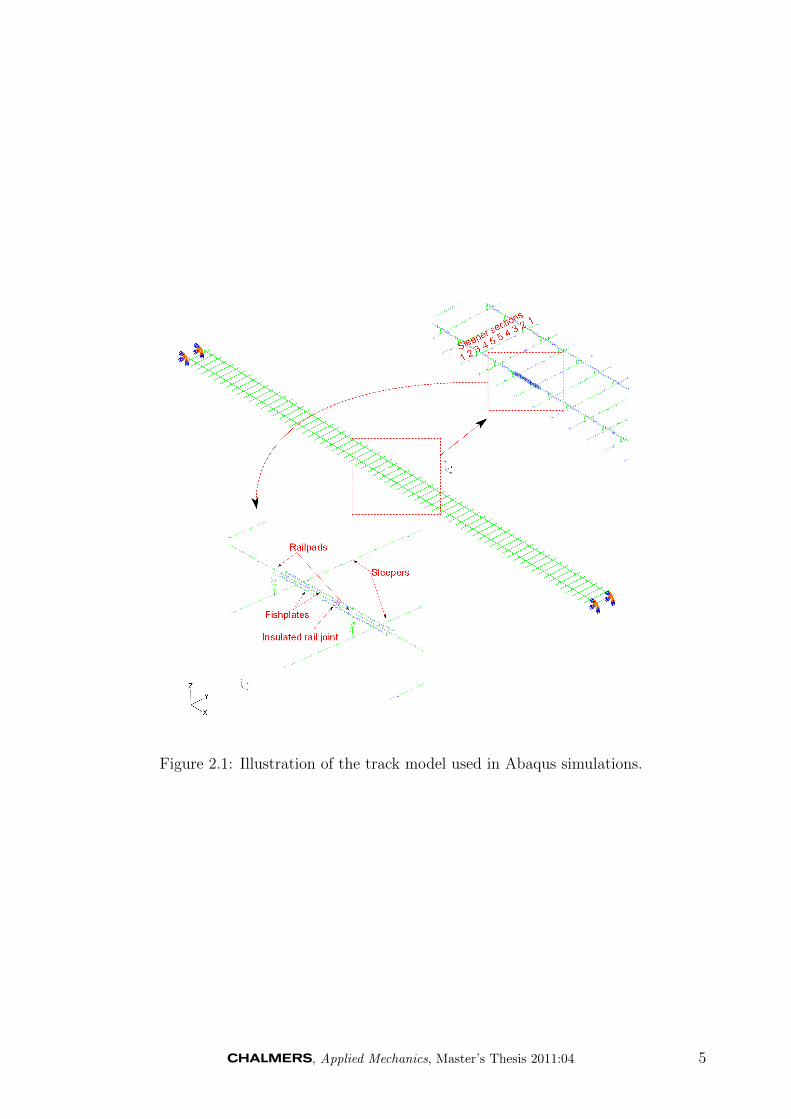
Figure 2.1: Illustration of the track model used in Abaqus simulations.


Figure 2.2: Location of bolt nodes used in the Abaqus model.

Figure 2.3: Zoomed in picture of rail 1 showing how the force is moved along the rail. Anidentical force with the same magnitude is applied on rail 2 (not shown in figure).


Figure 2.4: Illustration of the quasistatic approach in Abaqus for a bogie system with axledistance of 1 meter. There are five timesteps between each picture.

Figure 2.5: Maximum bending moment in fishplate given varying numbers of elements inthe fishplate.


Figure 2.6: Force convergence in element closest to first bolt, applied example load 10kN.

The shortest element lengths in the rail have here been employed close to the bolts.Two kinds of mesh convergence checks were used. Firstly all element lengths were reducedto check if the response distribution was similar. The refinements indicate that the meshis sufficiently dense to determine where the maxima are located.

Due to the refinement around the insulated joints, the element lengths are different inthe two rails, which results in that the forces of the left and right wheel are not applied atexactly the same coordinates along the rail. This is however not a big problem since theforce position on one rail does not have a major influence on the response in the other rail(the difference is less than 1%).

The mesh was thereafter refined in the regions where the responding forces were thehighest. The reason to confine the refinement to this region was to save computationaltime since the response in the intermediate regions was of less interest, the objective ofthe study was to localize the maxima, not to determine the exact response in every point.In figure 2.6 one can see that the force maxima converges in the studied regions, with amagnitude of the shear force range equal to the applied load, as expected (see table 2.3).

2.2 Investigated parameters

It is important to identify the parameters deemed most influential for joint degradation.In this project the axle distance (see chapter 3.1), the rail profile (3.3) and joint position(3.4) have been investigated. Dynamical effects from speed of the train and direction oftraffic have not been investigated but might be topics in follow-up projects.


Node distance at bolt 1 Maximal positive force Maximal negative force Force difference

30mm 1403N −7325N 8728N

10mm 1403N −8185N 9588N

2mm 1400N −8518N 9918N

0.4mm 1400N −8584N 9984N

Table 2.3: Force response in element closest to first bolt, applied example load 10kN.

3 Load modeling

In the simulations the loads acting on the rails have been applied as point loads in onenode per rail at each instant in time. The point of application is then moved along the rail.Based on the result of the convergence study (see chapter 2.1) the nodes are placed at aminimal distance of 17.5mm. Since the length of the actual contact pressure distribution inthe wheel-rail contact in practice could be at most some 30mm, and we are not evaluatingthe contact stress field but the bending moment in the rail, it is a reasonable simplificationto adopt point loads in the quasi-static simulation.

3.1 Single and double axle bogies

To evaluate the influence of the nearby wheelset in a bogie, and thus assess whetherthe bogie distance is of interest in the calculations, simulations with two different axledistances were carried out. The bogie load was modeled as four point loads (two on eachrail). These loads were then moved one node in each simulation increment, an illustrationof the procedure is shown in figure 2.4.

As can be seen in figure 3.1 the difference between the single bogie model and the doublebogie models is somewhat influenced by the different bogie distances. For distances of 3meters the maximum negative moment becomes larger and the maximum positive bendingmoment is almost identical to the single bogie situation. For an axle distance of 1 meterthe cycles interact so that the minimal bending moment between the positive peaks ispositive. If the rail profile is changed, the bending moment magnitude changes (see figure3.2) and hence also the effects of bogie distance.

Dynamic effects related to the different bogie distances might be larger. However, dy-namic effects are not considered in this study due to the complexity they include thatbasically makes any attempt at standardization futile, see further chapter 3.2.

Additionally, the aim of the project is to develop a standard for comparison betweendifferent insulated joint constructions subjected to loads that reflect the operational con-ditions. It is therefore not a primary concern to account for minor deviations due to thebogie construction, the main focus is to establish sufficiently realistic load scenarios underwhich the different joints can be tested and compared. The actual load conditions willthen vary depending on axle loads and speed (due to dynamic effects), bogie distances,support conditions etc.

Bogie distances affect the response, but it does not change the location of the criticalpoints.

Since the maximal moment is similar in all situations studied the conclusion from thispart of the investigation was to carry out the tests with loads corresponding to a singleaxle load system.


Figure 3.1: Bending moments for single and double bogie with axle distances of 1, 2 and3 meters.


Figure 3.2: Bending moments for rail profiles UIC60 and BV50.


3.2 Dynamic load effects

The loading generated by a moving vehicle on a rail can be divided into a (quasi-) staticand a dynamic contribution. The latter is governed by the dynamic response of the systemand influenced by parameters such as vehicle speed, sleeper spacing, dynamic propertiesof suspension etc. Thus, the dynamic contribution is strongly related to the operationalcharacteristics of the passing vehicles and also the rail foundation (sleepers, ballast etc).However, the aim of the current study is not to evaluate the loading of an insulated jointas accurately as possible, but rather to design a sufficiently realistic test set-up in whichdifferent insulated joints can be tested. For this reason, an analysis of the dynamic effectshas been excluded from the current study. This does of course not mean that insulatedjoints are not subjected to dynamic load effects. These may exist and may be significant,especially for run-down joints (see [5]). However they can be approximated by an increasein the applied static load magnitude.

It also does not mean that the dynamic load effects are the same for all insulated joints.They may vary depending on the design of the joint. This influence can be assessed ina separate analysis of the dynamical characteristics of the joint: The recommended testset-up (see 3.6) includes a step-increase of the applied loads. If one wants to roughlyevaluate the effects of dynamical load contributions, one could thus evaluate the responseat a higher load magnitude.

3.3 Rail profile

In Sweden, the two most frequently used rail profiles are UIC60 (60E1) and BV50 (50E3)(see figures 7.1, 7.2, 7.3 and 7.4). Simulations have been carried out to compare the result-ing bending moments and sectional forces in the joint components given the different railprofiles. As can be seen in figure 3.2 the results differ little between the two profiles regard-ing maximum bending moments, but somewhat more regarding the response distribution,which can be of interest if a double axle bogie model is used. In this project, as mentionedbefore, double axle bogie effects are not treated and therefore the difference between therail profiles is sufficiently small to be neglected in further calculations. Consequently, ifnothing else is stated, the BV50 profile is employed and analyzed below.

If for some reason more exact calibrations are needed, different test setups could beused for different rail profiles. However, as discussed above – the main aim is to establishsufficiently realistic test conditions that make tests of different joints comparable, not toexactly model the real situations.

3.4 Joint position

There are basically two philosophies of how the insulated joint shall be positioned, asshown in figure 3.3. When the joint is placed in the center of a sleeper span, the highestshear force in the full-scale model is found in bolt 2. It would however be desirable to havea testing procedure that is applicable for both positions of the joints. Since the materialstructure of the rail should be the same around both bolt 1 and 2 (the rail and fishplateprofiles are of same shapes, but the boundary conditions differs) it would be sufficient tojust measure on bolt 1 in the test even if it would be bolt 2 that gets the highest stress.In addition from a testing perspective it is easier to apply loads further apart from eachother, to apply loads on bolt 2 and over the area around the insulating material might betoo difficult to carry out.


Figure 3.3: Two common positions of the insulating joint relative to nearby sleepers.

3.5 Insulation material

Results from the literature [5] conclude that very limited amounts of the applied loadis carried by the insulating material. Consequently, the insulation layer is numericallymodeled as a gap in the current simulations. This simplification should have very smalleffect on the results since the elastic modulus of the joint is very low compared to that ofthe rail (2.5 · 109 and 2.1 · 1011N/m2, respectively).

3.6 Test specimen

The next step in developing a test set-up was to recommend a length of the test specimen.In addition it was important to conclude which load scheme that should be recommended,and which boundary conditions that would be feasible.

The boundary conditions were chosen as simply supported. The main reason was that itwould require very high clamping forces in the rail ends to maintain the beam inclinationand therefore it would have been difficult to make the tests reproducible and cost-effective.

To make it possible to accomplish the tests in as many labs as possible a goal was toreduce the length of the beam. The evaluation of a feasible beam length was based on ananalysis of where in the model the maximum force and the maximum bending momentarise. The next step would therefore be to design the test specimen such that the responsein the critical points would be as similar to the ”reality” as possible.

Instead of applying the load as a rolling wheel, which would have been both expensiveand inexact, the applied load was chosen as two point loads, one in each of the selectedcritical points (see figure 4.3). It is important that the load functions are not designed insuch way that the force and moment responses result in additional load cycles (see figure4.2). Except from that restriction, the time evolution of the loads is of less importance.According to fatigue design theory [2] the number of cycles to failure is related only to themaximum and mean load magnitude.

The loads are scaled such that the response (in terms of bending moment and shear forcemagnitude) corresponded to the complete rail structure. The reason why the two loads arenot scaled equally is that the point of application vary and thereby are differently affectedby the boundary conditions.

Since the shear force and bending moment ratios (min value divided by max value) differbetween the full-scale rail structure and the test set-up, this needs to be compensated for.


Maximum Minimum Equivalentmaximum

Quotient

Force in rail atbolt 1

−8600N 1400N 9270N 1.078

Bending mo-ment in fish-plate nearjoint

1077Nm −195Nm 1170Nm 1.086

Table 3.1: Maximum and minimum force at bolt and moment at joint for an applied forceof 10kN in the quasistatic FE simulation. From these magnitudes the equivalent maximaaccording to the Smith–Watson–Topper [4] criteria are calculated. Since the model islinear it is possible to scale the above values to desired level. The quotient is computed asEquivalent maximum/maximum.

To this end the Smith–Watson–Topper [4] criteria has been employed to evaluate equivalentforces and bending moments, see table 3.1.

There should be no complications related to the fact that the specimen only is loadedin two points and that measurements are made at two locations. This is because of theassumption that the areas around the bolts are assumed to behave in the same way andtherefore it is only important to apply load and measure the response in the most criticalpoint. It is important to ensure that the selected critical points are indeed the higheststressed.

3.7 Error margins

If the test specimen length is for some reason longer or shorter than proposed or if theloads are applied on other locations, it is important to predict if the structure behaves inanother way than if it is properly done. If the distance between the supports is increasedwith 0.01m in each end, the maximum bending moment is increased with less than 2% andif the beam length is decreased with 0.01m in each end the maximum bending momentdecreased with less than 2%. See figure 3.4.


Figure 3.4: Maximum bendin moment in test specimen for different lengths given anequivalent static force of 10kN .


4 Test setup

In Abaqus, a test specimen was modeled on which forces were applied in two points, seefigure 4.3. The aim is to get a similar force-response in the region close to bolt 1 and asimilar bending moment response in the region around the joint for the test specimen modelas compared to the quasi-static track model. To achieve this, two forces were applied, oneover bolt 1 and one over the joint. To model a situation similar to the quasi-static one theforces are to be applied as sinus-shaped waves as can be seen in figure 4.1 b), i.e. with aphase shift of half a period. The load on the joint starts when the load is maximum atbolt 1, and the load on bolt 1 reaches zero when the load is maximum at the joint.

In addition the set-up with two forces makes it less favorable to optimize only towardsbetter strength in one region (e.g. around the joint material / center of the fishplates).

4.1 Test procedure

The recommended test procedure is as follows: First the test is done with loads equiva-lent to 25 tonnes axle load for 200 000 cycles, thereafter the load is increased with stepsequivalent to 5 tonnes for 100 000 cycles each, see table 4.1. When the equivalent load hasreached 50 tonnes the test is run until breakage, or at most an additional 500 000 cycles.

Since the fatigue strength is independent of loading frequency and since the eigenfre-quency of the beam was computed to be around 197Hz which is much greater than what isfeasible in a laboratory, the frequency of the test can be chosen arbitrary. It is importantthat the frequencies of the two loading cycles are the same and that a phase shift as infigure 4.1 b) is adopted.

Between each change of load magnitude, photographes are to be taken to make it possibleto determine the specimen deterioration before break. Required photos are listed below.

Photographes to be taken between each load cycle:

1. From one side, perpendicular to the rail, at the joint

2. From the other side, perpendicular to the rail, at the joint

3. From one side, perpendicular to the rail, at bolt 1

4. From the other side, perpendicular to the rail, at bolt 1

5. From above on the joint

6. From below on the joint

7. From above on the point where the load is applied over bolt 1

8. From below the rail under bolt 1

Summary of load instructions:

1. At each increase in load magnitude the standardized electrical insulation test [7] shallbe done

2. Before the load cycles are started the given load on the joint shall be applied staticallyso that it is possible to measure the statical deformation of the rail.

3. The load cycles shall be sinus-shaped and pulsating (maxima equal to the double theamplitude)


Figure 4.1: Three different phase shift profiles with phase shift of 0.36, 0.5 and 0.81 ofthe period time, respectively. Figure 4.2 shows the bending moment response given thedifferent phase shifts.


Figure 4.2: Bending moment response given the different phase shifts shown in figure 4.1.Too small phase shift (green rhombus line) gives too high bending moment response. Ifthe phase shift is too large (red quadrat line) the bending moment response will containadditional load, which shorten the lifetime of the test specimen. Recommended phase shiftis half of the period time, which in this figure is represented by the blue line with circles.

Equivalentaxle load(tonnes)

Force over bolt 1 (N) Force over joint (N) Number of cycles

25 1.23 · 105 1.34 · 105 200 000

30 1.47 · 105 1.61 · 105 100 000

35 1.72 · 105 1.87 · 105 100 000

40 1.96 · 105 2.14 · 105 100 000

45 2.21 · 105 2.41 · 105 100 000

50 2.46 · 105 2.68 · 105 500 000∗

∗ The structure will probably break before reaching 500 000 cycles at this level, so it shallbe seen as an upper limit.

Table 4.1: Table of recommended load scheme.


Figure 4.3: Recommended test set-up for test specimen of profile BV50.

Figure 4.4: Recommended positions for strain-gauges and strain rosettes. See also figure4.5


Figure 4.5: Recommended positions for strain-gauge in profile view. See also figure 4.4

4. The load cycles over bolt and joint shall have the same period length

5. The load applied over the joint shall have half a period phase shift as compared tothe load applied over the bolt. First when the load over the joint has reached zeroa new load cycle shall begin over the bolt. This means that there is at least half aperiod between the pulses. See figure 4.1 b.


5 Evaluation of field validation tests

To conclude which type of insulated joint that gives the least amount of operational dis-ruptions (signalling errors) and the longest operational life-times statistical data have tobe compared.

When comparing different types of joints one type is considered as the reference (usuallythe model already in use) with which an alternative is compared. In the model presentedhere the different types of joints (e.g. two types – with 4mm and 6mm gaps) are treatedas two error-generating sources. Errors are here presumed as occur according to a Poissionprocess. The joints are not compared individually; it would be too difficult to measurethe performance of separate joints. Instead the two groups of joints (reference and ”new”)are compared. The comparison presumes that the groups are similarly affected from thesurrounding environment. It is therefore important that the joints to be compared areinstalled at the same time (and thus in different places) instead of comparing with thejoints that were placed at the same locations before. The reason is that both the jointsand the track degrade over time. In addition, operational conditions, such as tonnage,vehicle types and climate may change. Thus if the joints are not installed at the sametime, any comparison is very cumbersome. In particular comparing joints of different agewill be very misleading.

To compare the joints one option is to sort the joints into so called twin tests. Thisimplies that one combines the joints two and two such that each pair of joints (containingone ”reference” and one ”new” joint) has as equal surrounding and operational conditionsas possible. To conclude if there are any statistically significant differences between thetwo joint types the difference in error occurrence for each pair is used as the stochasticvariable. Although this is a very ”clean” approach, it would probably be too difficult sinceit is not obvious how to sort into similar joint configurations (average speed of passingtrains, average load, distance to station, frequency of passing trains etc).

The most practical way might instead be to randomly place the different joint typesto make all external disturbances as evenly distributed as possible between the two jointgroups. The randomness can be achieved as follows: First one determines all places wherethe joints shall be installed and the proportion of the two joint types (equal numbers ofeach type is not necessary but it makes the comparison easier). Then one randomizeswhich type of joint that shall be installed for each position. This procedure makes theexternal effects evenly spread from a statistical point of view and therefore the test morereliable.

The individual joints are not separately compared; instead the two types of joints aretreated as two independent entities. The occurrence of errors are expected to be Poissondistributed and the evaluation of the test is done by constructing a confidence interval forthe quotient of the failure intensities.

Here it should be noted that it is probably too difficult to carry out the analysis fora subdivision into different types of errors in the comparison. If deemed interesting, aseparate study can instead be made to establish whether the dominating error types varybetween the different joint types.

5.1 Determining which joint type that has the highest quality

To conclude if one of the joint types is more likely to generate errors, and therefore shouldbe avoided, one formulates a null hypothesis that λ1 = λ2, where λ1 = λ2 are the Poissonintensities for joints of type 1 and 2, respectively. If one can determine that the null hy-pothesis is false within a given confidence interval one concludes that there are statistically


Confidence interval Values for χ2(1)c

90% 2.706

95% 3.841

99% 6.635

Table 5.1: χ2-values for given confidence intervals. For a more detailed table, see [3]

significant differences in the failure probabilities. Following formula is then used [8]:

H0 : λ1 = λ2 (5.1)

Q =(n1 + n2)2

n1n2(x1 + x2)

(x1 −

n1(x1 + x2)

n1 + n2

)2

=

=(n1 + n2)2

n1n2(x1 + x2)

(n2x1 − n1x2

n1 + n2

)2

=

=(n2x1 − n1x2)2

n1n2(x1 + x2)(5.2)

Q(n1 = n2) =(x1 − x2)2

x1 + x2

(5.3)

λ1 Poisson intensity for joint type 1λ2 Poisson intensity for joint type 2n1 Number of joints of type 1n2 Number of joints of type 2x1 Number of errors generated by joint type 1 during the test periodx2 Number of errors generated by joint type 2 during the test periodx2c Required value of x2 to achieve a given confidence interval cχ2(1)c Value depending on given confidence interval, see table 5.1

If Q exceeds the prescribed values in column 2 of table 5.1 then the null hypothesisis false within a confidence interval of the value in column 1 on the corresponding row.The χ2-distribution is used since a division of Poisson variables is used and the degree offreedom of 1 is equal to the number of compared types minus 1 (one). To calculate therequired value x2c to achieve a confidence interval c for a given value of x1 the followingformula is used, given n1 = n2:

(x1 − x2c)2

x1 + x2c

> χ2(1)c

x22c − x2χ

2(1)c − 2x1x2c > x1χ2(1)c − x2

1(x2c −

(12χ2(1)c + x1

))> x1χ

2(1)c − x21 +

(12χ2(1)c + x1

)2

x22c >

12χ2(1)c + x1 +

√x1χ2(1)c − x2

1 +(

12χ2(1)c + x1

)2(5.4)

The formula shows greater significance the larger x1 and x2 are given same quota betweenthe numbers. Analogous to this the required quotient of x1 and x2 is lower the largerthe numbers become. For example, if n1 = n2, x1 = 10, x2 has to be 21 or higher toassure a 95% confidence interval for x2 > x1. If x1 = 100 then x2 has to be 130 for the


same confidence interval. This indicates that the higher the number of failures, the moresignificant results can be obtained in determining which of the two joint types that is moreprobable to generate errors.

It is possible to make more than one comparison, for example if one wants to know if aspecial type of insulated joint is more suitable for a specific situation. One should howeverbe careful not to divide the evaluation test into too small groups. As can be seen in table5.2 if one of the joints has generated 10 errors during the test period and the other onetwice as many (20) errors you do not even have a 95% confidence interval that the firstjoint is of higher quality. If you instead let the test run over a longer period of time and/orinclude more joints in the test so that one of the joint types generates 100 errors you can,within a 99% confidence interval conclude that this joint is of higher quality than the otherif the other one has generated twice as many (200) errors during the test period. Longertime intervals and more tested joints gives more robust conclusions as to whether one ofthe joints is more reliable than the other.

It is however possible, and recommendable to both compare error statistics on the wholeand error statistics for different parts of the validation study to identify any anomalies (e.g.,an excessive number of errors for a certain joint) that may not be related to the joint typein itself.

Conclusions for obtaining a high significance in validation testing:

• Remove external variables by randomizing the placement of the joints.

• Compare as few types of joints as possible, preferably only two types.

• Install the joints at same time to remove effects of weather, change in traffic etc.

• Include as many joints as economically and operationally possible – the more joints,the higher the significance of the test.

• Let the test continue over a long period of time, the longer the better. Preferablythe test should continue until all joints have reached their operational life and arereplaced or subjected to excessive revision. It might be that one type of joint isbetter in the short perspective in the sense that it generates less errors but insteadhas a shorter life-time. The results of such an analysis together with an analysis ofwhich joint type that is to be preferred – one with a long life-time or one with fewoperational errors – should form the decision for which joint type to adopt under agiven operational condition.

• Be sure to relate operational errors to the correct joint. If this cannot be done, thereliability in the evaluation is reduced.

• File the errors so that it can be possible after the tests to determine if special typesof joints are more suited for special locations etc. If possible, classify the error.

5.2 Quality factor comparison

The method above is not applicable to determine how big the difference is in qualitybetween the two types of joints, only to determine if you with a given confidence intervalcan conclude if one of the joints is less error prone than the other. To evaluate the actualdifference in quality could be of interest if the prices of the two joints are different and oneneeds to know if it is worth the higher price to reduce errors. For such a comparison, thefollowing methodology is used [8]:


Least number of x2 to achievegiven confidence interval

x1 90% 95% 99%

10 19 21 26

20 32 35 40

50 68 72 80

100 125 130 140

200 235 242 256

500 554 564 586

1000 1075 1090 1119

Table 5.2: Table of number of recorded errors required to achieve confidence intervals fordetermining which joint that is of highest quality.

H0 : f · λ1 = λ2 (5.5)

Q =(fx1 − x2)2

(x1 + x2)(5.6)

Where f is the factor of how much more erroneous the joint that has generated thehighest amount of errors is as compared to the other joint type. If f is 1.5 it means thatthe more erroneous joint in average generates 50% more errors than the less erroneousjoint. Then the following equations are used to determine the least required value of x2cf

(fx1 − x2cf )2

f(x1 + x2cf )> χ2(1)c

x22cf − fx2χ

2(1)c − 2fx1x2cf > fx1χ2(1)c − f 2x2

1(x2cf −

(12fχ2(1)c + fx1

))2> fx1χ

2(1)c − f 2x21 +

(12fχ2(1)c + fx1

)2

x22cf >

12fχ2(1)c + fx1 +

√fx1χ2(1)c − f 2x2

1 +(

12fχ2(1)c + fx1

)2

(5.7)

f Quality factor, see table 5.3x2cf Required number of x2 to achieve given confidence interval c if the quality factor

is set to f

In table 5.3 f -values of 1.1, 1.25 and 1.5 are used. If Q is higher than correspondingχ2(1)c-value one can reject H0 within a significance interval given by c. Some pre-calculatedvalues are given in table 5.3.

Example: Assume that you have two types of joints and one of the jointtypes (joint1) has generated 100 errors during the test period. If the other jointtype (joint2) has generated 145 errors during the same time period (which is≥ 142, see row 6, column 2 in table 5.3) errors during the same time periodyou can conclude within a 95% confidence interval that λ2 (the error densityvariable of joint2) is at least 10% higher than λ1. If x2 instead should havebeen 194 (≥ 191, see row 6, column 6) you would have had a 95% confidenceinterval that λ2 is at least 50% higher than λ1.


λ2/λ1 > 1.1 > 1.25 > 1.5

x1 95% 99% 95% 99% 95% 99%

10 23 28 26 31 31 37

20 41 48 43 49 51 58

50 79 88 89 98 105 116

100 142 153 161 173 191 206

200 265 280 299 316 357 376

500 619 642 701 726 838 867

1000 1197 1228 1357 1391 1623 1663

Table 5.3: Values for x2 required to achieve different confidence intervals for differentquotients of λ2/λ1. Calculated by equation 5.7

Normal distribution

Confidence interval c ac

90% 1.282

95% 1.645

99% 2.326

Table 5.4: Values for normal distribution parameter ac for different confidence intervals.

5.3 Mean life estimation

After the last joint has been replaced or been extensively revised it is possible to comparethe mean operational life of the two joint types. Here the two types are denoted x andy. To evaluate the confidence interval, the mean operational life is approximated as beingNormal distributed, see e.g. [1].

The joint with highest mean operational life during the test is denoted x. The lifetimesof the individual test joints are denoted xi, i = 1, ..., n and yj, j = 1, ...,m. From these,mean values x and y and variances s2

x and s2y are calculated as:

x =n∑i=1

xin

y =n∑i=1

yim

s2x =

∑(xi − x)2/(n− 1)

s2y =

∑(yi − y)2/(m− 1) (5.8)

Finally one can construct a confidence interval for the difference of the two expected meanlife times µx and µy. µx is greater than µy within a confidence interval of c if the followinginequality holds [6]:

x− y − ac ·√s2x

n+s2y

m≥ 0 (5.9)

Where ac is related to the Normal distribution as given in table 5.4.


5.3.1 Mean life time estimation, five joints of each type

Assume that there are 5 joints of type 1 and 5 of type 2 (n=5, m=5). The lifetimes arelisted in table 5.5.

Type1 Type2

5 4

6 5

7 6

8 7

9 8

Table 5.5: Lifetimes in years for two joint types.

x1 = 7, x2 = 6 Assume null hypothesis H0 that µ1 = µ2 Given 95% confidence, µx − µyis at least

x− y − a0.95 ·√s2x

n+s2y

m=

= 7 − 6 − 1.645 ·√

2.5

5+

2.5

5=

1 − 1.645 · 1 = −0.645 (5.10)

and since this value is not equal or greater than 0 the null hypothesis cannot be rejected.That means that we cannot with 95% certainity say that type 1 on average has a longeroperational life-time than type 2.

5.3.2 Mean life time estimation, 15 joints of each type

Assume instead that there are three times as many joints of each type, and that the lifetimesare distributed similar to the previous example. Life time distribution in this example isgiven in table 5.6.

For the same confidence interval as before (95%) µx − µy is at least

x− y − a0.95 ·√s2x

n+s2y

m=

= 7 − 6 − 1.645 ·√

2.143

15+

2.143

15=

= 1 − 1.645 · 0.535 = 0.121 (5.11)

since this value is greater than 0 the null hypothesis can be rejected within a 95%confidence interval, that is we can with 95% certainity say that type 1 on average has alonger operational life-time than type 2. This exemplifies how you can get more significantresults if you have more test objects.

5.4 Some simplifications and assumptions made in the abovestudy

Failure intensity is treated as constant over time. This assumption is made since no pre-knowledge exists on how failure intensities evolves over time. Failure intensity is also


Type1 Type2

5 4

5 4

5 4

6 5

6 5

6 5

7 6

7 6

7 6

8 7

8 7

8 7

9 8

9 8

9 8

Table 5.6: Lifetimes in years.

treated as unchanged by reparations. This is connected to the simplification that all kindof errors are treated equally in the statistics evaluation, and therefore it is not possible toinclude altered failure intensities after repair. No consideration is made regarding influenc-ing effects. However if the joints are randomly placed so that they on average are equallyaffected this should be no problem as discussed above.


6 Concluding remarks

6.1 Laboratory test set-up

It is important and inquired to have a standard for bending tests of insulated joints whichmakes it possible to compare different types of joints. This project is a step in thatdirection. The recommended test beam of length 1.17m should be sufficient to evaluate theperformance of different insulated joints under operational loading. Due to the relativelyshort length and simple boundary conditions, the test arrangement should be easy toaccomplish.

6.2 Validation tests

The statistical methods oulined in this report should be applicable in different comparisons,not only for insulated joints.


7 Appendix


Figure 7.1: Swedish railway administration’s drawing of rail profile BV50 / 50E3.


Figure 7.2: Swedish railway administration’s drawing of rail including fishplates for profileBV50 / 50E3.


Figure 7.3: Swedish railway administration’s drawing of rail profile UIC60 / 60E1.


Figure 7.4: Swedish railway administration’s drawing of rail including fishplates for profileUIC60 / 60E1.


References

[1] Gunnar Blom and Bjorn Holmquist. Statistikteori med tillampningar. Studentlitteratur,1998.

[2] Tore Dahlberg and Anders Ekberg. Failure Fracture Fatigue An Introduction. Stu-dentlitteratur, 2002.

[3] Lennart Rade and Bertil Westergren. Mathematics Handbook for Science and Engi-neering. Studentlitteratur, 2004.

[4] Norman E. Dowling. Mechanical behavior of materials. Pearson Education, Inc, 2007.

[5] Jens C O Nielsen Elena Kabo and Anders Ekberg. Alarm limits for wheel-rail impactloads – part 1: rail bending moments generated by wheel flats. Vehicle system dynamics,44:718–729, 2006.

[6] Urban Hjorth. Statistisk slutledning i ekonomi och praktik. Studentlitteratur, 1998.

[7] Fredrik Jansson. Trv 2010/87382 teknisk kravspecifikation for passraler med limmadeisolerskarvar, 2010.

[8] Igor Rychlik and Jesper Ryden. Probability and Risk Analysis An Introduction forEngineers. Springer, 2006.

[9] Dassault systems. Abaqus version 6.8. http://www.simulia.com, 2008.


http://www.simulia.com

validation of insulated joints - chalmers publication...

Documents