mary amiti and beata smarzynska javorcki - imf.org · wp/05/55 trade costs and location of foreign...

WP/05/55

Trade Costs and Location of Foreign Firms in China

Mary Amiti and

Beata Smarzynska Javorcki

© 2005 International Monetary Fund WP/05/55

IMF Working Paper

Research Department

Trade Costs and Location of Foreign Firms in China

Prepared by Mary Amiti and Beata Smarzynska Javorcki1

Authorized for distribution by Shang-Jin Wei

March 2005

Abstract

This Working Paper should not be reported as representing the views of the IMF. The views expressed in this Working Paper are those of the author(s) and do not necessarily represent those of the IMF or IMF policy. Working Papers describe research in progress by the author(s) and are published to elicit comments and to further debate.

This study examines the determinants of entry into by foreign firms, using information on 515 Chinese industries at the provincial level during 1998–2001. The analysis, rooted in the new economic geography, focuses on market and supplier access within and outside the province of entry, as well as production and trade costs. The results indicate that market and supplier access are the most important factors affecting foreign entry. Access to markets and suppliers in the province of entry matters more than access to the rest of China, which is consistent with market fragmentation due to underdeveloped transport infrastructure and informal trade barriers. JEL Classification Numbers: F1, F23 Keywords: Foreign direct investment, trade costs, market access, supply access Author(s) E-Mail Address: [email protected]; [email protected]

1 We would like to thank Caroline Freund, Mary Hallward-Driemeier, Will Martin, Stephen Redding, John Romalis, Tony Venables, Shang-Jin Wei, and participants at the Workshop on National Market Integration (World Bank and Development Research Council) in Bejing, September 2003, the Workshop on China’s Economic Geography and Regional Development in Hong Kong, December 2003, and the World Bank/IMF seminars for helpful comments and suggestions. We are also grateful to the China National Bureau of Statistics (NBS) and the China Customs Office for supplying us with the data, and to Sourafel Girma for providing some additional data.

- 2 -

Contents Page

I. Introduction.................................................................................................................3 II. Theory .........................................................................................................................5 III. Data and Measurement ...............................................................................................8 A. NBS Data ...........................................................................................................8 B. Entry and Exit of Foreign Firms ........................................................................9 C. Supplier Access..................................................................................................9 D. Market Access..................................................................................................10 E. Provincial Characteristics ................................................................................11 F. Model Specification .........................................................................................11 IV. Results.......................................................................................................................12

A. Sensitivity ........................................................................................................13 B. Extensions ........................................................................................................14 V. Conclusions...............................................................................................................14 Tables 1. Summary Statistics....................................................................................................16 2. Determinants of Foreign Entry .................................................................................17 3. Links to Domestic Firms...........................................................................................18 4. Domestic Market Oriented Firms .............................................................................19 5. Determinants of Foreign Entry - Extensions ............................................................20 Appendix Figures A.1 Net Entry of FIEs in Coastal Provinces in 2001.......................................................21 A.2 Net Entry of FIEs in Midland Provinces in 2001 .....................................................21 A.3 Net Entry of FIEs in Western Provinces in 2001......................................................22 Appendix Tables A.1 Industries with the Highest Net Entry of FIEs .........................................................23 References ..........................................................................................................................24

- 3 -

I. INTRODUCTION

Governments all over the world spend large sums of money to entice foreign direct investment(FDI), usually offering generous tax incentives. It is generally expected that foreign firms willgenerate positive externalities on domestic firms, particularly in developing countries. Forexample, Javorcik (2004) provides evidence consistent with the existence of positive inter-industryspillovers from foreign firms in Lithuania. However, the evidence on the success of tax incentivesin attracting FDI is rather mixed (see Desai and others 2004), which raises the question of whatfactors in fact influence where foreign firms locate.

The theoretical literature on firm location emphasizes a tension between production costs andaccess to large final goods markets and input suppliers. Recent work by Krugman and Venables(1995) and Markusen and Venables (1998, 2000) shows that while market size is an importantconsideration for firms, the higher number of firms in large markets bids up the cost of immobilefactors. The relative strength of these factors in determining location depends critically on tradecosts. The view that both market size and access to intermediate inputs affect foreign investors’decisions is supported by anecdotal evidence. For instance, a manager of Salcomp, a Finnishmobile phone company, justified the interest of the company in China by stating that “Our marketsare in China, our components are there and wages are much lower...” (Financial Times, May2004).

Building on the predictions of the theoretical literature on economic geography, this studyexamines the relative importance of market access, supplier access, trade costs, and factorcosts on the entry of foreign firms into China. While FDI determinants have been analyzedextensively (for example, see Caves, 1982; and Markusen, 1995), little attention has been paid tothe new economic geography aspects of the investment decision. Notable exceptions are studiesby Head and Mayer (2004) and Head and Ries (1996). The former study focuses on marketaccess and shows that there exists a positive correlation between entry of Japanese firms into theEuropean Union (EU) and market potential measures, which aggregate demand from multiple EUregions adjusted by distance. The latter study takes into account market and supplier access asdeterminants of foreign entry into China, but does not incorporate any spatial aspects. That is,their proxies for the availability of inputs are the total number of industrial enterprises and thetotal value of industrial output within the province of foreign entry in China.2

Our analysis extends the literature in several dimensions. First, we consider the importance ofboth market and supplier access in determining foreign entry, taking into account spatial aspects.We allow for the possibility that firms purchase inputs not only from within their own province,but also from other provinces within China and from the rest of the world. Second, our measuresof market and supplier access take into account the varying degrees of interindustry linkages.For example, proximity to a steel plant is likely to be more valuable to a car producer than atextile manufacturer. Third, by incorporating all the key factors highlighted in the new economic

2Head and Ries (1996) assume that firms buy all their inputs locally, and they do not distinguishin their analysis between various degrees of input availability in different industries.

- 4 -

geography literature, we are able to provide an assessment of the relative importance of productioncosts and market size effects in attracting new entry.

China is a particularly interesting country in which to analyze FDI flows. It was among thetop FDI recipients in the world during the period under study, receiving US$165 billion ofdirect investment flows between 1998 and 2001 (World Investment Report 2002, Annex TableB3). Rising inequality between Chinese provinces has been of growing concern to the Chinesegovernment which has introduced a number of policies aimed at mitigating this development.3

With over 90 percent of foreign investment being directed to the coastal regions, the influx of FDIhas widened regional disparities between coastal and central regions within China. By providingan assessment of the importance of market access and supplier access relative to productioncosts, this study provides some guidance on the kinds of policy instruments that would be mostsuccessful in attracting FDI to disadvantaged regions.

In addition to an intrinsic interest in determinants of FDI flows into China, our study sheds somelight on the economic impact of interprovincial barriers to trade. There exists evidence suggestingthat in an effort to protect industries from competition, local governments in China are erectingbarriers to entry of goods from other provinces. The presence of such barriers was reportedby Kumar (1994) and Young (2000) and is consistent with anecdotal evidence. For instance,managers of Chinese firms confirmed that they have indeed experienced some difficulties inaccessing markets in other provinces. A manager of a medical manufacturing plant reported thatthe shipments to other provinces are occasionally stopped by local rail officials for two to fourweeks for no apparent reason. The administrative units of the industry and commerce departmentwere reportedly obstructing access to markets through audits or local registration requirements.4Unfortunately, it is not possible to directly measure such barriers. As it is illegal to impose traderestrictions, the measures adopted to protect local industries from competition are usually moresubtle than a direct border tax. Thus the only way to assess the significance of such barriers isindirectly, as is the case in our study.5

Our analysis is based on a comprehensive data set provided by the China National Bureau

3Strong economic growth experienced by China during this time did not benefit all provincesequally. For instance, while in 1999 the GDP of coastal provinces increased by 7.2%, central andwestern provinces experienced a growth rate of only 3.8 and 4.7%, respectively. In the sameyear, coastal provinces accounted for 60% of Chinese GDP and almost three-quarters of nationaloutput of manufactured goods. See Amiti and Wen (2001) for a discussion on regional inequalityin earlier years and the spatial distribution of manufacturing industries in 1995.4Interviews with firms and government officials were conducted by Amiti in five differentprovinces in October 2001.5A number of researchers have tried to estimate the size of these provincial trade barriers usingindirect measures (see Poncet, 2003; Young, 2000; Naughton,1999; Huang and Wei, 2003; andBai and others, 2004), but none of them has considered the consequences of such barriers. Noneof the studies has ruled out the existence of provincial border barriers and some have foundevidence that such barriers have increased over time.

- 5 -

of Statistics (NBS) covering nearly all manufacturing industries, at a highly disaggregatedlevel (515 industries) in 29 Chinese provinces, during the period 1998–2001.6 Using theinformation on the value of output by industry and province, the national input/output table, andinter-provincial distances we construct measures of market access and supplier access. We alsocreate industry-specific measures of tariff rates on imported inputs. We then relate these measuresto the change in the number of foreign firms in each province and industry. We also control for avariety of provincial characteristics. Proxies for trade costs at the provincial level include transportinfrastructure and openness to international trade. Production costs are proxied by provincialwages and electricity prices. We consider separately market access and supplier access within andoutside the province of foreign entry. A lower magnitude of the coefficients pertaining to tradeoutside the province of entry relative to trade within the province would suggest that the internaltrade barriers may be restricting access of foreign investors to suppliers and customers in otherregions.

The results indicate that market access and supplier access are the most important factors affectingFDI inflows. Doubling either market access or supplier access is associated with a 40% increasein the entry of foreign firms. The presence of customers and suppliers in the province of entrymatters much more than market and supplier access to the rest of China, which is consistent withthe presence of interprovincial barriers to trade. Further, our analysis suggests that provinceswhich are more open to foreign trade attract more foreign firms. Similarly, the availability ofinfrastructure is positively correlated with foreign entry. Although production costs also play asignificant role in determining the location of foreign investment, the magnitude of these effectsis around half that of the market and supplier access effects. A doubling of wages or electricityprices reduces entry of foreign firms by 17% and 22%, respectively. Thus, our results suggestthat local governments may do well by reducing interprovincial barriers, and hence increasingthe extent of market and supplier access in surrounding provinces, in order to attract foreigninvestment.

The rest of the paper is organized as follows. Section II develops the formal model. Section IIIprovides background information on China and details of the data sources. Section IV presentsthe results, and section V concludes.

II. THEORY

We derive our estimating equation from a new economic geography model, based on Krugman

6Other studies on the determinants of FDI in China rely either on information on provincial FDIstocks (Cheng and Kwan, 2000), or on the Almanac of China’s Foreign Economic Relations andTrade which lists entry of individual firms (Head and Ries 1996, Dean, Lovely and Wang, 2002).The latter data set is, however, limited in coverage as it includes only about 10 percent of newforeign firms, focuses exclusively on joint ventures and stopped being published in 1996. It isalso unclear what criteria were used to select a particular sub-sample of all foreign investors forpublication.

- 6 -

and Venables (1995) and Amiti (2005).7 Firms are assumed to compete in a monopolisticallycompetitive environment, with each firm producing a differentiated variety. All varieties of finalgoods enter symmetrically into the consumer’s utility function and all varieties of intermediateinputs enter symmetrically in the firm’s cost function. Profits of a single representative firm inindustry i in province p are given by

πip = pipxip − wα

p rβp

¡P up

¢µi £bixip

¤− F. (1)

The total cost function comprises a fixed cost, F , a constant cost, bi, and factor prices, where wp

is the wage in province p, rp is the price of capital in province p or any other factor of production,and P u

p is the intermediate input price index. It is defined as

P up =

"PXl=1

nul¡pul t

ulp

¢1−σu# 11−σu

. (2)

The transport cost, tilp, of shipping a good from province l to p is modelled as Samuelsonianiceberg costs, with t ≥ 1. This means that a proportion of imported inputs, 1− 1

t, melts in transit.

Hence, to deliver one unit of any good from one province to another t units must be shipped asonly a fraction 1

tarrives. If t = 1 there is free trade and if t =∞ there is no trade.

The fob producer price is given by profit maximization, which gives the usual marginal revenueequals marginal cost condition, with prices proportional to marginal cost:

pip = wαp r

βp

¡P up

¢µibiθi, θi =

σi

σi − 1. (3)

The mark-up over marginal cost, θi, depends on the elasticity of substitution σi.

Output of each firm in industry i in province p, xip, is sold to consumers and firms located withinprovince p, in other provinces within China, and to the rest of the world. Product market clearingconditions give

xip =PXl=1

cipl +CXc=1

cipw. (4)

Demand for industry i goods produced in province p is given by

cipl =¡pip¢−σi ¡

tipl¢1−σi

Eil

¡P il

¢σi−1. (5)

7Amiti (2005) extends Krugman and Venables (1995) from a one-factor model to a two-factormodel, thus allowing for different production stages to vary in factor intensities.

- 7 -

Expenditure on industry i, Ei, not only comes from consumers but also from downstream firms,

Eil = silYl + µindl p

dl x

dl . (6)

Downstream firms spend a proportion µ of their total revenue, ndl pdl xdl , on goods produced byindustry i (the second term in equation 6). Demand from downstream firms is derived usingShepard’s lemma on the price index (as shown in Dixit and Stiglitz, 1977).

Summing across all locations within China and the rest of the world, we derive aggregate demand,and setting it equal to supply gives

xip =¡pip¢−σi ( PX

l=1

¡tipl¢1−σi

Eil

¡P il

¢σi−1+

WXp=1

¡tipw¢1−σi

Eiw

¡P iw

¢σi−1

). (7)

Substituting in the product market clearing condition (7) and the profit maximizing price (3) intothe profit function, (1), gives

πip =³wαp r

βp

¡P up

¢µi´1−σi ¡θi − 1

¢ ¡θi¢1−σi "(P+WX

l=1

¡tipl¢1−σi

Eil

¡P il

¢σi−1

)#− F. (8)

It is assumed that free entry and exit of firms ensures zero profits in equilibrium. Firms enter whenprofits are positive and exit when profits are negative. Any exogenous changes to, say, trade costswould affect profits and hence the number of firms in each location. We allow all variables to betime varying hence entry can be written as a function of the change in profits:

∆nip = nip,t − nip,t−1 = f(πip,t − πip,t−1). (9)

Note that profits, inclusive of the fixed cost π0 = π + F , if F is small then ln(π + F ) ' ln(π),hence taking natural logs of equation 8 we have8

lnπip,t = αi(1− σi) lnwp,t + β(1− σi) ln rp,t + µ(1− σi) lnP up,t (10)

+νI + νt + ln

(P+WXl=1

¡tipl¢1−σi

Eil

¡P il

¢σi−1

),

where νI represents industry fixed effects such as the degree of market power, θi, and νt representstime fixed effects. Taking first differences, denoted by ∆, these fixed effects are eliminated, and

8Note that in Krugman and Venables (1995), the fixed cost is also a function of the factor pricesand the intermediate input price index. To simplify the equation, we assume that foreign firms paya fixed cost with resources from the parent company.

- 8 -

our estimating equation becomes

∆nip,t = γ0 + γ1∆ lnwp,t + γ2∆ ln rp,t + γ3∆ lnP up,t (11)

+γ4∆ ln

(P+WXl=1

¡tipl,t¢1−σi

Eil,t

¡P il,t

¢σi−1

).

Thus in our empirical analysis we include average wages varying by province and time. Thetheory predicts a negative coefficient on wages, that is other things equal, firms prefer to locatein provinces that offer lower wages. As in the model, we assume that new entrants are too smallindividually to influence the provincial wage, so they take it as given. We also assume thatthe supply of workers in each province is given and workers are immobile between provincesand mobile between industries within a province. Thus in effect, we are treating each provinceanalogously to a country in the theoretical model. This assumption is a reasonable approximationin China, given the hukou system.9 The other province specific costs rp could include any otherfactors of production whose costs vary across provinces, for example electricity prices. Transportcost are modelled as a function of distance. Transport costs can also be affected by the availabilityof infrastructure, such as the number of sea berths, river berths, and lengths of railroads, which weinclude separately.

Our key variables of interest are market and supply access variables. We hypothesize thatprofits are positively related to better access to intermediate inputs, which are reflected in alower intermediate input price index, P u

p , which we will proxy by three different supplier accessvariables; and that firms are also concerned about good market access, reflected in the last term,which we will proxy by various market access variables. We define these variables in the nextsection.

III. DATA AND MEASUREMENT

A. NBS Data

The data used in the analysis have been collected by the China National Bureau of Statistics(NBS) at the firm level and then aggregated up to 600 industries by province, based on the 4 digitChinese Industrial Classification. Before releasing this data to us, the NBS removed all “sensitiveindustries” from the sample, and then we excluded agriculture, extractive industries and servicesin order to focus on the manufacturing sector. The information available includes the number offoreign firms, the value of output of foreign firms and the value of output of domestic firms. Allvariables vary by province, sector and time. Our sample covers the 1998-2001 period. It wasnot possible to include earlier years in the sample as data on the number of foreign firms wereunavailable.

The figures indicate that a vast majority of foreign entry in 2001 occurred in coastal provinces(see Appendix). Seven out of twelve provinces in the coastal region saw the number of foreign

9The hukou is a system of residence permits that regulates the movement of labor.

- 9 -

investment projects rising by more than a hundred. Guangdong and Zhejiang were the mostsuccessful provinces increasing the number of foreign investment enterprises (FIEs) by about 600each. Although midland provinces received much less net foreign investment, some province likeHunan recorded a net entry as high as 40, similar to some of the coastal provinces such as Beijing.

In terms of distribution of net entry across industries, both sectors producing consumer goodsand industrial parts and components appeared to be attractive to foreign investors. The moreattractive consumer industries included paper products, household plastic products, lamps andlanterns, and cotton knitting, while in the industrial categories there was a lot of foreign activityin electronic elements and automobile fittings and parts. In 2000 and 2001, manufacturing ofclothing (classification 1810) experienced the largest rise in the number of foreign projects, from160 to 260. See Table A.1 for details.

Foreign investment enterprises account for a significant share of industrial output produced inChina. In 2001 their share in total production was equal to 31.3 percent. The share of FIEs inprovincial output ranged from 2.4 percent in Xinjiang to 58 percent in Tianjin, 65 in Fujian and61 in Guangdong in 2001. In twenty sectors (out of 515 considered in our sample), foreignenterprises accounted for three-quarters or more of industrial output produced in China in 2001.These included some technology intensive industries, such as manufacturing of copying machines,computers, cameras and instruments, communication equipment, radio and tape recorders,integrated circuits as well as consumer good industries – processing of fish sauce and productionof soft drinks.

B. Entry and Exit of Foreign Firms

The dependent variable in our model is defined as the change in the number of foreign firmsoperating in industry i, province p, at time t, or in other words the net entry of foreign firms:∆nip,t = nip,t − nip,t−1. The variable is positive if the number of firms that entered is greater thanthe number of firms that exited; zero if there has been no change or the number of new firmsexactly equals the number of exiting firms; and negative if the number of exiting firms exceededthe number of new entrants.10

C. Supplier Access

We construct three measures of supplier access. The first one is SA_ownip,t which captures theavailability of inputs used by industry i in province p where it is operating:

SA_ownip,t =KXk=1

aikY kp,t

Y kCHINA,t

∗DIST−1pp , (12)

where Y kp,t is the output of industry k produced in province p at time t. It is divided by the total

output of industry k produced in China, to get the share of output of each industry k producedin each province. Since industries use more than one intermediate input, these output shares are

1020% of the observations are non-zero.

- 10 -

weighted by aik, which are the coefficients from the China national input-output (I/O) table for1997. Given that this is the most recent I/O table available, we assumed that the technology isconstant throughout the sample period. There is variation in the supplier access variables dueto entry and exit of firms. There are 70 manufacturing I/O codes, which we concord with theindustrial data. Thus, while we analyze entry for 515 industries, our proxies for supplier accessare defined for 70 I/O codes. In order to make this variable comparable with the proxy for inputavailability in other provinces (SA_outerip,t) we adjust it for the within province distance, which

is defined as DISTpp =q

Areapπ

.

The availability of intermediate inputs in the rest of China is proxied by

SA_outerip,t =KXk=1

aik

PXl 6=p

Y kl,t

Y kCHINA,t

∗DIST−1lp , (13)

which is analogous to the own province supplier access measure. To take account of the additionalcost of accessing inputs from other provinces, we weight the output shares produced in eachprovince by the inverse of distance from province p to province l. While this measure is intendedto capture the cost of transporting intermediate inputs it may also, to some extent, reflect localprotectionism.

The importance of intermediate supplies from the rest of the world is proxied by trade weightedtariffs imposed by China on imported intermediate inputs, weighted by the I/O coefficient aik, toreflect the fact that the relative importance of inputs varies by industry,

SA_abroadit =KXk=1

aik ∗ tariffskt . (14)

The information on trade weighted tariffs on products corresponding to the I/O codes comes fromthe World Bank’s World Integrated Trade Solution (WITS) database. It should be noted that manyindustries in China have access to duty free intermediate inputs through duty drawbacks and hencewould not be affected by tariffs on intermediate inputs. Nonetheless, there are many industriesthat do pay these tariffs and thus it is important to include this variable in the estimation.11

D. Market Access

We construct two measures of market access to reflect that firms can supply other firms andhouseholds within their own province and in other provinces. The own market access measure isdefined as

MA_ownip,t =

"KXk=1

bikY kp,t

Y kCHINA,t

+ biGDPp,t

GDPCHINA,t

#∗DIST−1

pp , (15)

11Approximately 40 per cent of imports are subject to tariffs.

- 11 -

where Y kp,t is the output of industry k produced in province p at time t. It is divided by the total

output of industry k produced in China, to get the share of industry k’s output produced in eachprovince. The share is then weighted by bik, which is the fraction of industry i’s output sold toindustry k as intermediate input, and bi is the fraction sold for final consumption to households.

Note thatKXk=1

bik + bi = 1. The coefficients bik and bi have been calculated based on the China

national I/O table for 1997.

Similarly, market access to the rest of China is defined as

MA_outerip,t =KXk=1

bik

PXl 6=p

Y kl,t

Y kCHINA,t

∗DIST−1lp + bi

PXl 6=p

GDPl,t

GDPCHINA,t

∗DIST−1lp , (16)

where each province’s consumption of industry’s i’s output is weighted by the inverse of distance.

E. Provincial characteristics

In addition to distance as a proxy for trade costs, we include in the estimation the number ofriver and sea berths and length of railroads, using information from the China Annual StatisticalYearbooks. The degree of openness of a province is constructed from international trade data fromthe Chinese Customs Office. The production cost variables at the provincial level include data onelectricity prices and wages obtained from the NBS. Wages are calculated as the ratio of the totalwage bill to employment by province and year. We include all locations in China except Tibetand Inner Mongolia because the latter two have very little industrial activity. This gives us 29locations comprising 25 provinces and 4 directly administered cities: Shanghai, Beijing, Tianjinand Chongqing. Table 1 provides summary statistics of all the variables.

F. Model Specification

Substituting in the proxies for supplier and market access, our estimating equation (11) can berewritten as

∆ni,p,t = α + βSA ln(SA_ownip,t + βSA_outerSA_outerip,t)

(SA_ownip,t−1 + βSA_outerSA_outerip,t−1)(17)

+βMA ln(MA_ownip,t + βMA_outerMA_outerip,t)

(MA_ownip,t−1 + βMA_outerMA_outerip,t−1)

+βSA_abroad∆ lnSA_abroadip,t + ∆ lnXp,tβ + εip,t.

We estimate equation (17) using ordinary least squares (OLS), omitting the outer terms, andwith nonlinear least squares (NLS), adjusting standard errors for clustering on I/O-code-yearcombinations. Since market access and supplier access variables tend to be highly correlated, in

- 12 -

addition to the full specification presented above we also estimate models with only market accessor supplier access variables.

IV. RESULTS

The results, presented in Table 2, confirm the importance of proximity to markets and suppliers.We present both OLS and NLS results in all the Tables to illustrate the importance of links to otherprovinces.12 Comparing the ols results in columns (1) to (3) to the nls results in columns (4) to(6), we see that the magnitudes of the coefficients on market access and supplier access variablesare much higher in the nls estimations, where we take account of access to other provinces.Comparing columns (1) and (4), where both market access and supplier access are included, thecoefficient on MA increases from 0.16 to 1.14, and the coefficient on SA increases from 0.26 to1.09, which suggests that access to other provinces is important for entry. Note that even thoughsome of the access variables are individually insignificant in column (4), F-tests indicate they arejointly significant with a p−value equal to 0. In columns (5) and (6), we reestimate the equationwith only SA in column (5) and only MA in column (6). Here we see that the coefficients on SAand MA are even larger than when they are included jointly, which is likely due to the correlationbetween the terms. Using estimates from column (4) with the full specification, the results indicatethat a doubling of either market access or supplier access increases the entry of foreign firms by0.8, and evaluated at the mean number of foreign firms (equal to 1.87), this is equivalent to a 40%increase in the number of foreign firms in an industry/province.

Interestingly, both the outer terms on market access and supplier access are positive and less thenone. Since both own and outer supplier access have been adjusted for distance, the parameterβSA_outer allows us to compare the relative magnitude of the two effects. A coefficient belowone would suggest that the presence of suppliers in other provinces is less important that theability to source within the own province. This indeed is the case as βSA_outer equals 0.14 incolumn (4); and the coefficient on βMA_outer is 0.42, which implies that outer supplier accessis approximately 14% of the total supplier access effect, and the outer market access effect isapproximately 40 percent of the total market access effect. This finding suggests that firms mayface some difficulties with accessing inputs and selling their products in neighboring provinceseither due to high transport costs and/or interprovincial barriers to trade.

Since foreign investors may also import some of their inputs, the model controls for the averagetariff charged on inputs used by industry i and the province’s openness to trade (defined asthe share of provincial imports and exports to GDP). As hypothesized, the average tariff bearsa negative sign, while openness to trade is positively correlated with foreign entry. Bothvariables are significant in all six specifications, which suggests that ease of access to importedintermediates is important to foreign investors.

12This also serves as an additional robustness test – the fact that coefficients on all the othervariables are similiar in both specifications adds confidence that the nonlinear estimations are infact global minima rather than local ones.

- 13 -

Production costs are also crucial in determining where foreign firms locate. As anticipated, thecoefficient on the average provincial wage is negative and significant suggesting that foreigninvestors are attracted to locations with lower labor costs. Further, provinces with cheaperelectricity appear to be more attractive as an investment destination. In all specifications in Table2, the coefficient on wage is equal to -0.6 and on electricity around -0.45. Thus a doubling ofproduction costs decreases foreign entry between 17% and 22%, respectively. This is about halfthe size of the effect of doubling either MA or SA.

The availability of infrastructure plays a role in the entry decision as well. The higher the numberof sea berths or the length of railroads the higher the foreign entry. The number of river berths, onthe other hand, appears to have a very small negative effect. The length of rail has the largest effectout of the infrastructure variables, with a coefficient equal to 0.85. This implies that doubling railincreases foreign entry by 32%, suggesting that transport costs are indeed a significant factor indetermining entry.

A. Sensitivity

Links to Domestic Firms To ensure that the output of the new entrants is not driving theresults, we reconstruct the MA and SA variables using only the output of domestic firms. Ideally,we would only purge the variables of the output of those new foreign entrants, however, sinceour data are at the industry level this information is not available. One drawback of removing allforeign output in the access variables is that it may be omitting important inter-industry linkagesin industries that may be dominated by foreign firms. The results are presented in Table 3. We seethat the inclusion of these domestic oriented linkage terms increases the size of the SA variablesand reduces the size of the MA variables. The coefficients on all other variables are very similarto the earlier estimates. In this case, it appears that the high correlation between MA and SAvariables may be affecting the MA coefficients when all of them are included, as the hypothesisthat βMA_own = βMA_outer = 0 cannot be rejected in column (4). Yet the F-test of the jointsignificance of the MA terms when they are included on their own as in column (6) indicates jointsignificance with a p-value equal to 0. The two SA coefficients have a higher magnitude thanbefore with both terms being statistically significant in column (5), which suggests that accessto inputs purchased from domestic firms is relatively more important than those purchased fromother foreign firms.

Domestic Oriented Foreign Firms The ability to sell products within China is likely tomatter less for export-oriented investors. Thus, to check the robustness of our earlier findings were-estimate the above models restricting the sample to industry-province-year combinations whereless than 30 percent of output is exported (see Table 4). The export-orientation of a given industryin a particular province is calculated by summing the value of exports of all firms operating in agiven industry, province and year combination and dividing it by the sum of the total production inthe same cell. If an observation for a particular year is missing it is substituted with an observation

- 14 -

for the closest year available.13 The results confirm our earlier findings. The effects of the MAand SA variables are of similar magnitudes to the previous results. Although the coefficients are abit smaller than in the full sample, they range between 0.6 and 0.7, as compared to 1.1 in Table 2,they correspond to a similar sized effect when evaluated at the mean number of firms: doublingSA is associated with a 51% increase in entry when evaluated at the mean number of foreign firmswhich is equal to one in this sub-sample, and doubling MA is associated with a 44% increase.

The signs and significance levels of other variables remain unchanged. To ensure that ourresults are not driven by choosing the cutoff at 30 percent, we also estimate the model forindustry-province-year combinations where the share of exported output is less than 50 percent.The conclusions with respect to our key variables remain unchanged.

B. Extensions

In Table 5, we explore the effect of additional controls for distance to port14 and the investmentclimate in the province, proxied by the total number of foreign firms in the province lagged oneperiod. The results suggest that provinces close to ports appear to be more attractive investmentdestinations, which is not surprising, since as we discussed earlier, coastal regions have been theprimary recipients of FDI in China. The negative coefficient in this first differenced equationsuggests that distance to ports has become more important over time.

The ‘total foreign firms’ variable is defined as the total number of foreign firms in all industriesin a province, rather than a particular industry as is the case with the dependent variable, andit enters as a one period lag. The coefficient is positive and significant. Provinces with a largenumber of foreign firms are more attractive to new entrants either due to agglomeration benefits ordue to a better investment climate that attracted the other firms. It seems that the competition forresources or congestion externalities have not yet outweighed the benefits of being in a provincewith many other foreign firms present. Controlling for distance to ports and the lagged number offoreign firms reduces the market access effects slightly but leaves the supplier access coefficientsunchanged.

V. CONCLUSION

This study examines factors driving entry of foreign firms in China, using a comprehensivedata set covering nearly all manufacturing industries at the provincial level during the period1998–2001. The analysis is based on a new economic geography model, and thus focuses on theimportance of market and supplier access effects both within and outside the province of entry,relative to production costs.

13This data series has been provided by Sourafel Girma. See Girma and Gong (2004) for detailedinformation on the data source.

14This is measured as the shortest distance to one of the three major ports: Shanghai, Hong KongSAR, and Qinhuangdao (Hebei).

- 15 -

The findings suggest that access to customers and suppliers of intermediate inputs are the keydeterminants of FDI inflows. The analysis also highlights the importance of taking into accountlinkages to neighboring regions. After allowing for such linkages, the effects of market andsupplier access increase significantly. The results show that doubling either market access orsupplier access is associated with a 40% increase in the entry of foreign firms, whereas the effectof doubling production costs reduces entry of foreign firms by roughly 20%.

The analysis also shows that the presence of customers and suppliers in the province of entrymatters much more than market and supplier access to the rest of China. This may be due to theunderdeveloped transport infrastructure and informal barriers to trade and is consistent with thefragmentation of the Chinese market.

Other trade costs also appear to play an important role in attracting FDI. For instance, theavailability of infrastructure, such as rail lines, is positively correlated with foreign entry, whereashigh tariffs on imported inputs deter entry. Provinces which are more open to foreign trade attractmore foreign firms. In sum, barriers to trade whether in the form on tariffs on imported inputs,informal barriers to inter-provincial trade or underdeveloped infrastructure play a significant rolein the decisions of foreign investors contemplating entry into China.

If China’s central government is serious about redressing regional inequality, it must address theissue of local protection and high internal trade costs. Dismantling interprovincial barriers, andimproving transport infrastructure will increase market and supplier access for both Chinese andforeign producers, attracting entry of new firms.

- 16 -

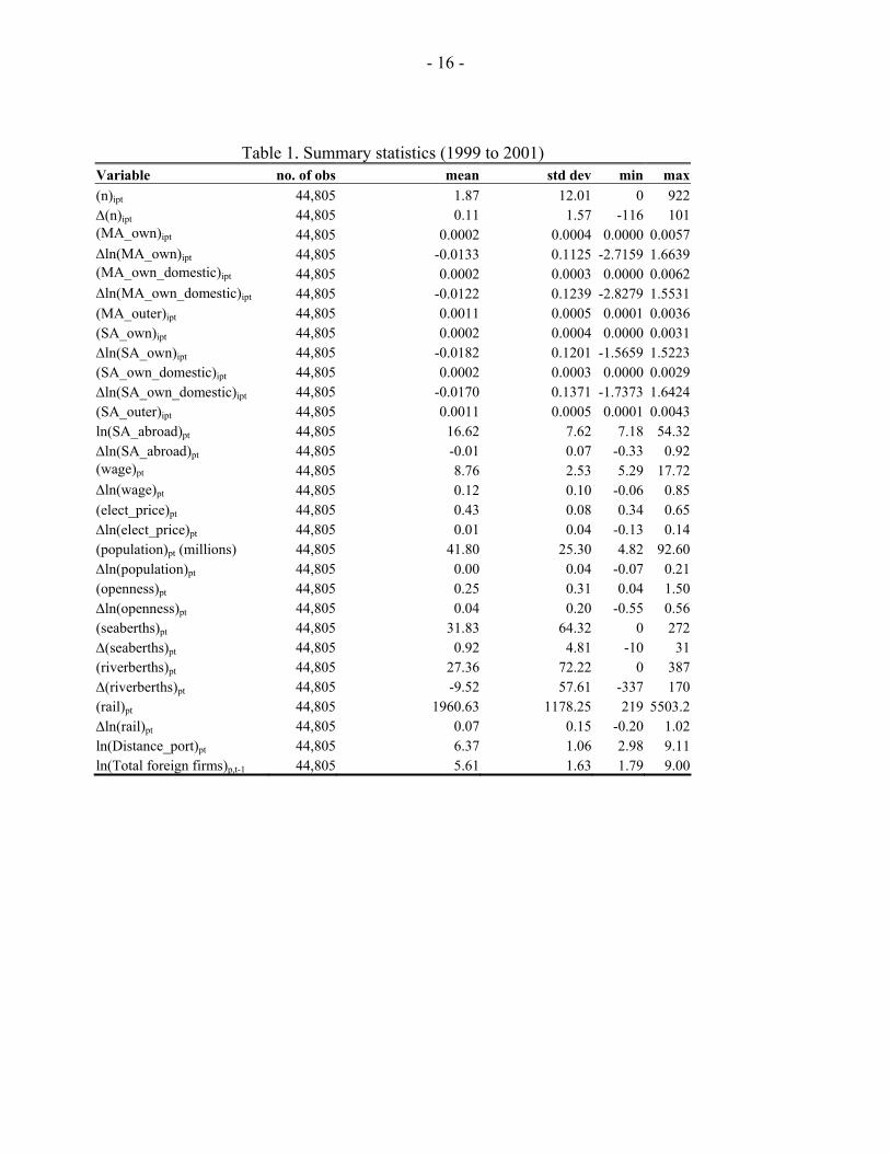
Table 1. Summary statistics (1999 to 2001) Variable no. of obs mean std dev min max (n)ipt 44,805 1.87 12.01 0 922 ∆(n)ipt 44,805 0.11 1.57 -116 101 (MA_own)ipt 44,805 0.0002 0.0004 0.0000 0.0057 ∆ln(MA_own)ipt 44,805 -0.0133 0.1125 -2.7159 1.6639 (MA_own_domestic)ipt 44,805 0.0002 0.0003 0.0000 0.0062 ∆ln(MA_own_domestic)ipt 44,805 -0.0122 0.1239 -2.8279 1.5531 (MA_outer)ipt 44,805 0.0011 0.0005 0.0001 0.0036 (SA_own)ipt 44,805 0.0002 0.0004 0.0000 0.0031 ∆ln(SA_own)ipt 44,805 -0.0182 0.1201 -1.5659 1.5223 (SA_own_domestic)ipt 44,805 0.0002 0.0003 0.0000 0.0029 ∆ln(SA_own_domestic)ipt 44,805 -0.0170 0.1371 -1.7373 1.6424 (SA_outer)ipt 44,805 0.0011 0.0005 0.0001 0.0043 ln(SA_abroad)pt 44,805 16.62 7.62 7.18 54.32 ∆ln(SA_abroad)pt 44,805 -0.01 0.07 -0.33 0.92 (wage)pt 44,805 8.76 2.53 5.29 17.72 ∆ln(wage)pt 44,805 0.12 0.10 -0.06 0.85 (elect_price)pt 44,805 0.43 0.08 0.34 0.65 ∆ln(elect_price)pt 44,805 0.01 0.04 -0.13 0.14 (population)pt (millions) 44,805 41.80 25.30 4.82 92.60 ∆ln(population)pt 44,805 0.00 0.04 -0.07 0.21 (openness)pt 44,805 0.25 0.31 0.04 1.50 ∆ln(openness)pt 44,805 0.04 0.20 -0.55 0.56 (seaberths)pt 44,805 31.83 64.32 0 272 ∆(seaberths)pt 44,805 0.92 4.81 -10 31 (riverberths)pt 44,805 27.36 72.22 0 387 ∆(riverberths)pt 44,805 -9.52 57.61 -337 170 (rail)pt 44,805 1960.63 1178.25 219 5503.2 ∆ln(rail)pt 44,805 0.07 0.15 -0.20 1.02 ln(Distance_port)pt 44,805 6.37 1.06 2.98 9.11 ln(Total foreign firms)p,t-1 44,805 5.61 1.63 1.79 9.00

- 17 -

Table 2. Determinants of Foreign Entry

Dependent Variable: ∆(n)ipt (1) (2) (3) (4) (5) (6) ols ols ols nls nls nls ∆ln(MA_own)ipt 0.159** 0.258*** 1.144 1.774*** (0.072) (0.082) (0.865) (0.752) (MA_outer)ipt

c 0.424 0.356 (0.477) (0.249) ∆ln(SA_own)ipt 0.269*** 0.321*** 1.094** 1.463*** (0.054) (0.054) (0.553) (0.539) (SA_outer)ipt

c 0.142 0.168* (0.113) (0.095) ∆ln(SA_abroad)pt -0.353** -0.354** -0.360** -0.364*** -0.364*** -0.364*** (0.143) (0.145) (0.139) (0.140) (0.141) (0.139) ∆ln (wage)pt -0.595*** -0.596*** -0.603*** -0.602*** -0.603*** -0.605*** (0.097) (0.097) (0.098) (0.097) (0.097) (0.097) ∆ln(elect_price)pt -0.473** -0.489*** -0.463** -0.419** -0.432*** -0.447*** (0.185) (0.184) (0.187) (0.182) (0.182) (0.185) ∆ln(population)pt 1.271*** 1.292*** 1.285*** 1.376*** 1.376*** 1.349*** (0.353) (0.354) (0.354) (0.355) (0.356) (0.356) ∆ln(openness)pt 0.182*** 0.180*** 0.180*** 0.176*** 0.176*** 0.176*** (0.067) (0.067) (0.066) (0.066) (0.066) (0.066) ∆ln(seaberths)pt 0.010*** 0.010*** 0.010*** 0.010*** 0.010*** 0.010*** (0.003) (0.003) (0.003) (0.003) (0.003) (0.003) ∆ln(riverberths)pt -0.0002** -0.0002* -0.0002* -0.0003** -0.0002** -0.0002* (0.0001) (0.0001) (0.0001) (0.0001) (0.0001) (0.0001) ∆ln(rail)pt 0.852*** 0.853*** 0.851*** 0.848*** 0.852*** 0.846*** (0.178) (0.178) (0.178) (0.177) (0.177) (0.178) H0: βMA_outer=0; βSA_outer=0 F=18.73

p-value=0 H0: βMA_own=0; βMA_outer=0 F=5.53

p-value=0 H0: βSA_own=0; βSA_outer=0 F=15.42

p-value=0 RSS 108778.96 108791.50 108819.98 108688.05 108714.87 108762.89 Observations 44805 44805 44805 44805 44805 44805 Notes: a)* significant at 10%; ** significant at 5%; *** significant at 1%; b) Robust standard errors corrected for clustering in parentheses; c) MA_outer and SAouter terms enter non-linearly as in equation (3.6).

- 18 -

Table 3. Links to Domestic Firms

Dependent Variable: ∆(n)ipt (1) (2) (3) (4) (5) (6) ols ols ols nls nls nls ∆ln(MA_own)ipt 0.072 0.139** 0.1071 0.7878 (0.046) (0.055) (0.771) (0.513) (MA_outer)ipt

c 0.780 0.315 (7.364) (0.304) ∆ln(SA_own)ipt 0.167*** 0.191*** 1.414 1.451** (0.056) (0.058) (0.881) (0.679) (SA_outer)ipt

c 0.4648 0.4672* (0.341) (0.273) ∆ln(SA_abroad)pt -0.358** -0.359** -0.361** -0.367*** -0.367*** -0.365*** (0.143) (0.144) (0.140) (0.141) (0.141) (0.139) ∆ln (wage)pt -0.596*** -0.596*** -0.604*** -0.601*** -0.601*** -0.605*** (0.096) (0.096) (0.098) (0.098) (0.097) (0.097) ∆ln(elect_price)pt -0.476** -0.485*** -0.470** -0.430*** -0.431*** -0.456*** (0.186) (0.186) (0.187) (0.183) (0.184) (0.185) ∆ln(population)pt 1.309*** 1.316*** 1.312*** 1.389*** 1.388*** 1.353*** (0.353) (0.353) (0.355) (0.356) (0.355) (0.358) ∆ln(openness)pt 0.179*** 0.178*** 0.178*** 0.181*** 0.180*** 0.177*** (0.067) (0.067) (0.066) (0.067) (0.067) (0.066) ∆ln(seaberths)pt 0.011*** 0.011*** 0.011*** 0.011*** 0.011*** 0.011*** (0.003) (0.003) (0.003) (0.003) (0.003) (0.003) ∆ln(riverberths)pt -0.0002* -0.0002* -0.0002* -0.0002* -0.0002* -0.0002* (0.0001) (0.0001) (0.0001) (0.0001) (0.0001) (0.0001) ∆ln(rail)pt 0.858*** 0.857*** 0.856*** 0.858*** 0.858*** 0.855*** (0.178) (0.178) (0.178) (0.177) (0.177) (0.178) H0: βMA_outer=0; βSA_outer=0 F=11.82


p-value=0.96 F=6.53

p-value=0 H0: βSA_own=0; βSA_outer=0 F=12.19


- 19 -

Table 4. Domestic Market-oriented Foreign Firms

Dependent Variable: ∆(n)ipt (1) (2) (3) (4) (5) (6) ols ols ols nls nls nls ∆ln(MA_own)ipt 0.069* 0.122*** 0.640 0.950* (0.035) (0.040) (0.585) (0.521) (MA_outer)ipt

c 0.915 0.476 (1.116) (0.388) ∆ln(SA_own)ipt 0.149*** 0.171*** 0.732* 0.940** (0.032) (0.031) (0.412) (0.413) (SA_outer)ipt

c 0.177 0.226 (0.144) (0.140) ∆ln(SA_abroad)pt -0.117* -0.118* -0.122** -0.124** -0.124** -0.125** (0.061) (0.062) (0.060) (0.060) (0.060) (0.060) ∆ln (wage)pt -0.202*** -0.202*** -0.206*** -0.207*** -0.207*** -0.208*** (0.050) (0.050) (0.050) (0.050) (0.050) (0.050) ∆ln(elect_price)pt -0.228** -0.236** -0.219** -0.200** -0.204** -0.213** (0.094) (0.094) (0.095) (0.093) (0.093) (0.095) ∆ln(population)pt 0.436** 0.447** 0.446** 0.497*** 0.497*** 0.481*** (0.187) (0.186) (0.187) (0.188) (0.188) (0.187) ∆ln(openness)pt 0.077** 0.076** 0.075** 0.075** 0.074** 0.074** (0.035) (0.035) (0.035) (0.035) (0.035) (0.035) ∆ln(seaberths)pt 0.006*** 0.006*** 0.006*** 0.006*** 0.006*** 0.006*** (0.002) (0.002) (0.002) (0.002) (0.002) (0.002) ∆ln(riverberths)pt -0.000 -0.000 0.000 0.000 0.000 0.000 (0.000) (0.000) (0.000) (0.0001) (0.0001) (0.0001) ∆ln(rail)pt 0.272*** 0.272*** 0.271*** 0.268*** 0.270*** 0.268*** (0.090) (0.090) (0.090) (0.090) (0.090) (0.090) H0: βMA_outer=0; βSA_outer=0 F=15.72


p-value=0.08 H0: βSA_own=0; βSA_outer=0 F=16.61


- 20 -

Table 5. Determinants of Foreign Entry – Extensions

Dependent Variable: ∆(n)ipt (1) (2) (3) (4) (5) (6) ols ols ols nls nls nls ∆ln(MA_own)ipt 0.130* 0.200*** 0.818 1.380** (0.066) (0.071) (0.760) (0.663) (MA_outer)ipt

c 0.290 0.273 (0.424) (0.219) ∆ln(SA_own)ipt 0.197*** 0.239*** 1.019* 1.312*** (0.052) (0.051) (0.550) (0.514) (SA_outer)ipt

c 0.144 0.159 (0.124) (0.098) ∆ln(SA_abroad)pt -0.271** -0.272** -0.275** -0.279*** -0.277*** -0.279*** (0.119) (0.120) (0.116) (0.117) (0.118) (0.116) ∆ln (wage)pt -0.474*** -0.475*** -0.481*** -0.475*** -0.476*** -0.479*** (0.086) (0.086) (0.086) (0.085) (0.086) (0.086) ∆ln(elect_price)pt -0.226 -0.238 -0.212 -0.178 -0.189 -0.197 (0.151) (0.150) (0.153) (0.149) (0.148) (0.152) ∆ln(population)pt 0.505 0.518 0.498 0.591* 0.579* 0.555 (0.337) (0.337) (0.339) (0.341) (0.340) (0.341) ∆ln(openness)pt 0.214*** 0.213*** 0.214*** 0.208*** 0.210*** 0.209*** (0.063) (0.063) (0.062) (0.062) (0.062) (0.062) ∆ln(seaberths)pt 0.006* 0.006* 0.006* 0.006* 0.006* 0.006* (0.003) (0.003) (0.003) (0.003) (0.003) (0.003) ∆ln(riverberths)pt -0.000* -0.000* -0.000* -0.0002** -0.0002** -0.0002* (0.000) (0.000) (0.000) (0.000) (0.000) (0.000) ∆ln(rail)pt 0.814*** 0.815*** 0.812*** 0.810*** 0.813*** 0.808*** (0.176) (0.175) (0.176) (0.175) (0.175) (0.175) (Distance_port)pt -0.042*** -0.042*** -0.040*** -0.045*** -0.044*** -0.042*** (0.011) (0.011) (0.011) (0.011) (0.011) (0.011) (Total foreign 0.045*** 0.046*** 0.048*** 0.044*** 0.045*** 0.046***

firms)p,t-1 (0.011) (0.011) (0.011) (0.011) (0.011) (0.011) H0: βMA_outer=0; βSA_outer=0 F=17.43


p-value=0.02 H0: βSA_own=0; βSA_outer=0 F=11.82


APPENDIX

- 21 -

Figure A.1. Net Entry of FIEs in Coastal Provinces in 2001

-100

0

100

200

300

400

500

600

700

Guang

dong

Zhejia

ng

Jiang

su

Shang

hai

Shand

ong

Fujian

Tianjin

Hebei

Guang

xi

Beijing

Liaon

ing

Hainan

No.

of f

irms

Figure A.2. Net Entry of FIEs in Midland Provinces in 2001

-10-505

1015202530354045

Hunan

Henan

Jiang

xi

Chong

qing

Shaan

xi

Heilon

gjian

g

Shanx

i

No.

of f

irms

APPENDIX

- 22 -

Figure A.3. Net Entry of FIEs in Western Provinces in 2001

-10

-5

0

5

10

15

20

Sichuan Guizhou Gansu Yunnan Qinghai Xinjiang Ningxia

No.

of f

irms

APPENDIX

- 23 -

Table A.1. Industries with the Highest Net Entry of Foreign Investment Enterprises (FIEs)

Rank Year Industry code Industry description Net entry1 2001 1810 Manufacture of clothing 260

2 2000 1810 Manufacture of clothing 160

3 2001 4160 Manufacture of electronic elements 131

4 2000 4160 Manufacture of electronic elements 83

5 2001 2230 Manufacture of paper products 79

6 2001 3070 Manufacture of household plastic products 70

7 2000 3727 Manufacture of automobile fittings and parts 69

8 2001 3727 Manufacture of automobile fittings and parts 64

9 2001 4073 Manufacture of lamp and lanterns 59

10 2001 1781 Manufacture of cotton knitting 58

11 1999 3090 Manufacture of other plastic products 51

12 2001 1390 Processing of other food 48

13 2001 1790 Other textile industry 48

14 2001 3434 Manufacture of abrasive tools 48 15 2001 2312 Printing of packing , decorating 47

- 24 -

REFERENCES

Amiti, Mary, 2005, "Location of Vertically Linked Industries: Agglomeration versus ComparativeAdvantage," European Economic Review, Vol. 49, No. 4, pp. 809–832.

————–, and Mei Wen, 2001, "Spatial Distribution of Manufacturing in China", in Modellingthe Chinese Economy, ed.by P.J. Lloyd and X.G. Zhang, (Cheltenham, UK: Edward Elgar).

Bai, Chong-En, Yingjuan Du, Zhigang Tao and Sarah Y. Tong, 2004, "Local Protection andRegional Specialization: Evidence from China’s Industries," Journal of InternationalEconomics, Vol. 63, pp. 397–417.

Caves, Richard E., 1982, Multinational Enterprise and Economic Analysis (New York:Cambridge University Press).

Cheng, Leonard K., and Yum K. Kwan, 2000,"What Are the Determinants of the Location ofForeign Direct Investment? The Chinese Experience," Journal of International Economics,Vol. 51, pp. 379–400.

Dean, Judith M., Mary E. Lovely, Hua Wang, 2002, "Foreign Direct Investment and PollutionHavens: Evaluating the Evidence from China" (unpublished; Washington: US InternationalTrade Commission).

Desai, Mihir A., Fritz C. Foley, and James R. Hines, Jr., 2004, "Foreign Direct Investment in aWorld of Multiple Taxes," Journal of Public Economics Vol. 88, pp. 2727–44.

Girma, Sourafel, and Yundan Gong, 2004, "Are there FDI-Generated Externalities to ChineseState-Owned Enterprises?" (unpublished; Leicester: University of Leicester).

Head, Keith, and John Ries, 1996, "Inter-City Competition for Foreign Investment: Static andDynamic Effects of China’s Incentive Areas," Journal of Urban Economics, Vol. 40, pp.38–60.

Head, Keith, and Thierry Mayer, 2004, "Market Potential and the Location of Japanese Investmentin the European Union" Review of Economics and Statistics, Vol. 86, No. 4, pp. 959–972.

Huang, Lin, and Shang-Jin Wei, 2002, "One China, Many Kingdoms? Using IndividualProduct Prices to Understand Local Protectionism in China", (unpublished; Washington:International Monetary Fund).

Javorcik, Beata S., 2004,."Does Foreign Direct Investment Increase the Productivity of DomesticFirms? In Search of Spillovers through Backward Linkages," American Economic Review,Vol. 93, pp. 605–627.

Krugman, Paul, and Anthony J. Venables, 1995, "Globalization and the Inequality of Nations,"Quarterly Journal of Economics, Vol. 110, pp. 857–880.

Kumar, Anjali, 1994, "China: Internal Market Development and Regulation," World BankCountry Study, Washington DC: World Bank.

Markusen, James R., 1995, "The Boundaries of Multinational Enterprises and the Theory ofInternational Trade," Journal of Economic Perspectives, Vol.9, No. 2, pp.169–189.

- 25 -

Markusen, James R,. and Anthony J. Venables, 2000, "The Theory of Endowment, Intra-industryand Multinational Trade," Journal of International Economics, Vol. 52, pp. 209–234.

——————, 1998, "Multinational Firms and New Trade Theory," Journal of InternationalEconomics Vol.46, pp. 183–203.

Naughton, Barry, 1999, "How Much Can Regional Integration Do to Unify China’s Market?"(unpublished; San Diego: University of California).

Poncet, Sandra, 2003, "Measuring Chinese Domestic and International Integration," ChinaEconomic Review Vol. 14, pp. 1-21.

Young, Alwyn, 2000, "The Razor’s Edge: Distortions and Incremental Reform in the People’sRepublic of China," Quarterly Journal of Economics, Vol. 115, pp.1091–1135.

World Investment Report, 2002, Transnational Corporations and Export Competitiveness, (NewYork: United Nations).

mary amiti and beata smarzynska javorcki - imf.org · wp/05/55 trade costs and location of foreign...

Documents