mark woodard - testbanklive.com · university of colorado at denver lyle cochran ......
TRANSCRIPT

INSTRUCTOR’S SOLUTIONS MANUAL
SINGLE VARIABLE MARK WOODARD
Furman University
CALCULUS SECOND EDITION
William Briggs University of Colorado at Denver
Lyle Cochran Whitworth University
Bernard Gillett University of Colorado at Boulder
with the assistance of
Eric Schulz Walla Walla Community College
Boston Columbus Indianapolis New York San Francisco Upper Saddle River
Amsterdam Cape Town Dubai London Madrid Milan Munich Paris Montreal Toronto Delhi Mexico City São Paulo Sydney Hong Kong Seoul Singapore Taipei Tokyo

The author and publisher of this book have used their best efforts in preparing this book. These efforts include the development, research, and testing of the theories and programs to determine their effectiveness. The author and publisher make no warranty of any kind, expressed or implied, with regard to these programs or the documentation contained in this book. The author and publisher shall not be liable in any event for incidental or consequential damages in connection with, or arising out of, the furnishing, performance, or use of these programs. Reproduced by Pearson from electronic files supplied by the author. Copyright © 2015, 2011 Pearson Education, Inc. Publishing as Pearson, 75 Arlington Street, Boston, MA 02116. All rights reserved. No part of this publication may be reproduced, stored in a retrieval system, or transmitted, in any form or by any means, electronic, mechanical, photocopying, recording, or otherwise, without the prior written permission of the publisher. Printed in the United States of America. ISBN-13: 978-0-321-95485-5 ISBN-10: 0-321-95485-8 1 2 3 4 5 6 OPM 17 16 15 14 www.pearsonhighered.com

Contents
1 Functions 5
1.1 Review of Functions . . . . . . . . . . . . . . . . . . . . . . . . . . . . . . . . . . . . . . . . . 5
1.2 Representing Functions . . . . . . . . . . . . . . . . . . . . . . . . . . . . . . . . . . . . . . . 15
1.3 Trigonometric Functions . . . . . . . . . . . . . . . . . . . . . . . . . . . . . . . . . . . . . . 31
Chapter One Review . . . . . . . . . . . . . . . . . . . . . . . . . . . . . . . . . . . . . . . . . . . . 39
2 Limits 47
2.1 The Idea of Limits . . . . . . . . . . . . . . . . . . . . . . . . . . . . . . . . . . . . . . . . . . 47
2.2 Definitions of Limits . . . . . . . . . . . . . . . . . . . . . . . . . . . . . . . . . . . . . . . . . 52
2.3 Techniques for Computing Limits . . . . . . . . . . . . . . . . . . . . . . . . . . . . . . . . . 60
2.4 Infinite Limits . . . . . . . . . . . . . . . . . . . . . . . . . . . . . . . . . . . . . . . . . . . . 68
2.5 Limits at Infinity . . . . . . . . . . . . . . . . . . . . . . . . . . . . . . . . . . . . . . . . . . . 74
2.6 Continuity . . . . . . . . . . . . . . . . . . . . . . . . . . . . . . . . . . . . . . . . . . . . . . 83
2.7 Precise Definitions of Limits . . . . . . . . . . . . . . . . . . . . . . . . . . . . . . . . . . . . 94
Chapter Two Review . . . . . . . . . . . . . . . . . . . . . . . . . . . . . . . . . . . . . . . . . . . . 101
3 Derivatives 109
3.1 Introducing the Derivative . . . . . . . . . . . . . . . . . . . . . . . . . . . . . . . . . . . . . 109
3.2 Working with Derivatives . . . . . . . . . . . . . . . . . . . . . . . . . . . . . . . . . . . . . . 120
3.3 Rules of Differentiation . . . . . . . . . . . . . . . . . . . . . . . . . . . . . . . . . . . . . . . 131
3.4 The Product and Quotient Rules . . . . . . . . . . . . . . . . . . . . . . . . . . . . . . . . . . 137
3.5 Derivatives of Trigonometric Functions . . . . . . . . . . . . . . . . . . . . . . . . . . . . . . 145
3.6 Derivatives as Rates of Change . . . . . . . . . . . . . . . . . . . . . . . . . . . . . . . . . . . 154
3.7 The Chain Rule . . . . . . . . . . . . . . . . . . . . . . . . . . . . . . . . . . . . . . . . . . . 167
3.8 Implicit Differentiation . . . . . . . . . . . . . . . . . . . . . . . . . . . . . . . . . . . . . . . 178
3.9 Related Rates . . . . . . . . . . . . . . . . . . . . . . . . . . . . . . . . . . . . . . . . . . . . 193
Chapter Three Review . . . . . . . . . . . . . . . . . . . . . . . . . . . . . . . . . . . . . . . . . . . 203
4 Applications of the Derivative 213
4.1 Maxima and Minima . . . . . . . . . . . . . . . . . . . . . . . . . . . . . . . . . . . . . . . . 213
4.2 What Derivatives Tell Us . . . . . . . . . . . . . . . . . . . . . . . . . . . . . . . . . . . . . . 229
4.3 Graphing Functions . . . . . . . . . . . . . . . . . . . . . . . . . . . . . . . . . . . . . . . . . 246
4.4 Optimization Problems . . . . . . . . . . . . . . . . . . . . . . . . . . . . . . . . . . . . . . . 278
4.5 Linear Approximation and Differentials . . . . . . . . . . . . . . . . . . . . . . . . . . . . . . 296
4.6 Mean Value Theorem . . . . . . . . . . . . . . . . . . . . . . . . . . . . . . . . . . . . . . . . 305
4.7 L’Hopital’s Rule . . . . . . . . . . . . . . . . . . . . . . . . . . . . . . . . . . . . . . . . . . . 310
4.8 Newton’s Method . . . . . . . . . . . . . . . . . . . . . . . . . . . . . . . . . . . . . . . . . . 316
4.9 Antiderivatives . . . . . . . . . . . . . . . . . . . . . . . . . . . . . . . . . . . . . . . . . . . . 329
Chapter Four Review . . . . . . . . . . . . . . . . . . . . . . . . . . . . . . . . . . . . . . . . . . . 338
1

2 Contents
5 Integration 3515.1 Approximating Areas under Curves . . . . . . . . . . . . . . . . . . . . . . . . . . . . . . . . 3515.2 Definite Integrals . . . . . . . . . . . . . . . . . . . . . . . . . . . . . . . . . . . . . . . . . . . 3705.3 Fundamental Theorem of Calculus . . . . . . . . . . . . . . . . . . . . . . . . . . . . . . . . . 3855.4 Working with Integrals . . . . . . . . . . . . . . . . . . . . . . . . . . . . . . . . . . . . . . . 4015.5 Substitution Rule . . . . . . . . . . . . . . . . . . . . . . . . . . . . . . . . . . . . . . . . . . 412Chapter Five Review . . . . . . . . . . . . . . . . . . . . . . . . . . . . . . . . . . . . . . . . . . . . 422
6 Applications of Integration 4356.1 Velocity and Net Change . . . . . . . . . . . . . . . . . . . . . . . . . . . . . . . . . . . . . . 4356.2 Regions Between Curves . . . . . . . . . . . . . . . . . . . . . . . . . . . . . . . . . . . . . . 4526.3 Volume by Slicing . . . . . . . . . . . . . . . . . . . . . . . . . . . . . . . . . . . . . . . . . . 4686.4 Volume by Shells . . . . . . . . . . . . . . . . . . . . . . . . . . . . . . . . . . . . . . . . . . . 4766.5 Length of Curves . . . . . . . . . . . . . . . . . . . . . . . . . . . . . . . . . . . . . . . . . . . 4856.6 Surface Area . . . . . . . . . . . . . . . . . . . . . . . . . . . . . . . . . . . . . . . . . . . . . 4906.7 Physical Applications . . . . . . . . . . . . . . . . . . . . . . . . . . . . . . . . . . . . . . . . 494Chapter Six Review . . . . . . . . . . . . . . . . . . . . . . . . . . . . . . . . . . . . . . . . . . . . 503
7 Logarithmic and Exponential Functions 5157.1 Inverse Functions . . . . . . . . . . . . . . . . . . . . . . . . . . . . . . . . . . . . . . . . . . 5157.2 The Natural Logarithmic and Exponential Functions . . . . . . . . . . . . . . . . . . . . . . 5267.3 Logarithmic and Exponential Functions with Other Bases . . . . . . . . . . . . . . . . . . . . 5387.4 Exponential Models . . . . . . . . . . . . . . . . . . . . . . . . . . . . . . . . . . . . . . . . . 5467.5 Inverse Trigonometric Functions . . . . . . . . . . . . . . . . . . . . . . . . . . . . . . . . . . 5517.6 L’Hopital’s Rule and Growth Rates of Functions . . . . . . . . . . . . . . . . . . . . . . . . . 5627.7 Hyperbolic Functions . . . . . . . . . . . . . . . . . . . . . . . . . . . . . . . . . . . . . . . . 570Chapter Seven Review . . . . . . . . . . . . . . . . . . . . . . . . . . . . . . . . . . . . . . . . . . . 580
8 Integration Techniques 5958.1 Basic Approaches . . . . . . . . . . . . . . . . . . . . . . . . . . . . . . . . . . . . . . . . . . 5958.2 Integration by Parts . . . . . . . . . . . . . . . . . . . . . . . . . . . . . . . . . . . . . . . . . 6018.3 Trigonometric Integrals . . . . . . . . . . . . . . . . . . . . . . . . . . . . . . . . . . . . . . . 6168.4 Trigonometric Substitutions . . . . . . . . . . . . . . . . . . . . . . . . . . . . . . . . . . . . 6258.5 Partial Fractions . . . . . . . . . . . . . . . . . . . . . . . . . . . . . . . . . . . . . . . . . . . 6428.6 Other Integration Strategies . . . . . . . . . . . . . . . . . . . . . . . . . . . . . . . . . . . . 6588.7 Numerical Integration . . . . . . . . . . . . . . . . . . . . . . . . . . . . . . . . . . . . . . . . 6678.8 Improper Integrals . . . . . . . . . . . . . . . . . . . . . . . . . . . . . . . . . . . . . . . . . . 6758.9 Introduction to Differential Equations . . . . . . . . . . . . . . . . . . . . . . . . . . . . . . . 688Chapter Eight Review . . . . . . . . . . . . . . . . . . . . . . . . . . . . . . . . . . . . . . . . . . . 696
9 Sequences and Infinite Series 7139.1 An Overview . . . . . . . . . . . . . . . . . . . . . . . . . . . . . . . . . . . . . . . . . . . . . 7139.2 Sequences . . . . . . . . . . . . . . . . . . . . . . . . . . . . . . . . . . . . . . . . . . . . . . . 7209.3 Infinite Series . . . . . . . . . . . . . . . . . . . . . . . . . . . . . . . . . . . . . . . . . . . . . 7339.4 The Divergence and Integral Tests . . . . . . . . . . . . . . . . . . . . . . . . . . . . . . . . . 7449.5 The Ratio, Root, and Comparison Tests . . . . . . . . . . . . . . . . . . . . . . . . . . . . . . 7539.6 Alternating Series . . . . . . . . . . . . . . . . . . . . . . . . . . . . . . . . . . . . . . . . . . 759Chapter Nine Review . . . . . . . . . . . . . . . . . . . . . . . . . . . . . . . . . . . . . . . . . . . 765
10 Power Series 77310.1 Approximating Functions With Polynomials . . . . . . . . . . . . . . . . . . . . . . . . . . . 77310.2 Properties of Power Series . . . . . . . . . . . . . . . . . . . . . . . . . . . . . . . . . . . . . 79210.3 Taylor Series . . . . . . . . . . . . . . . . . . . . . . . . . . . . . . . . . . . . . . . . . . . . . 79910.4 Working with Taylor Series . . . . . . . . . . . . . . . . . . . . . . . . . . . . . . . . . . . . . 810Chapter Ten Review . . . . . . . . . . . . . . . . . . . . . . . . . . . . . . . . . . . . . . . . . . . . 821
Copyright c© 2015 Pearson Education, Inc.

Contents 3
11 Parametric and Polar Curves 82911.1 Parametric Equations . . . . . . . . . . . . . . . . . . . . . . . . . . . . . . . . . . . . . . . . 82911.2 Polar Coordinates . . . . . . . . . . . . . . . . . . . . . . . . . . . . . . . . . . . . . . . . . . 84911.3 Calculus in Polar Coordinates . . . . . . . . . . . . . . . . . . . . . . . . . . . . . . . . . . . 86911.4 Conic Sections . . . . . . . . . . . . . . . . . . . . . . . . . . . . . . . . . . . . . . . . . . . . 881Chapter Eleven Review . . . . . . . . . . . . . . . . . . . . . . . . . . . . . . . . . . . . . . . . . . 901
Appendix A 919
Copyright c© 2015 Pearson Education, Inc.
4 Contents
Copyright c© 2015 Pearson Education, Inc.

Chapter 1
Functions
1.1 Review of Functions
1.1.1 A function is a rule which assigns each domain element to a unique range element. The independentvariable is associated with the domain, while the dependent variable is associated with the range.
1.1.2 The independent variable belongs to the domain, while the dependent variable belongs to the range.
1.1.3 The vertical line test is used to determine whether a given graph represents a function. (Specifically,it tests whether the variable associated with the vertical axis is a function of the variable associated withthe horizontal axis.) If every vertical line which intersects the graph does so in exactly one point, then thegiven graph represents a function. If any vertical line x = a intersects the curve in more than one point,then there is more than one range value for the domain value x = a, so the given curve does not represent afunction.
1.1.4 f(2) = 123+1 = 1
9 . f(y2) = 1
(y2)3+1 = 1y6+1 .
1.1.5 Item i. is true while item ii. isn’t necessarily true. In the definition of function, item i. is stipulated.However, item ii. need not be true – for example, the function f(x) = x2 has two different domain valuesassociated with the one range value 4, because f(2) = f(−2) = 4.
1.1.6 (f ◦ g)(x) = f(g(x)) = f(x3 − 2) =√x3 − 2
(g ◦ f)(x) = g(f(x)) = g(√x) = x3/2 − 2.
(f ◦ f)(x) = f(f(x)) = f(√x) =
√√x = 4
√x.
(g ◦ g)(x) = g(g(x)) = g(x3 − 2) = (x3 − 2)3 − 2 = x9 − 6x6 + 12x3 − 10
1.1.7 f(g(2)) = f(−2) = f(2) = 2. The fact that f(−2) = f(2) follows from the fact that f is an evenfunction.
g(f(−2)) = g(f(2)) = g(2) = −2.
1.1.8 The domain of f ◦ g is the subset of the domain of g whose range is in the domain of f . Thus, weneed to look for elements x in the domain of g so that g(x) is in the domain of f .
1.1.9
When f is an even function, we have f(−x) = f(x)for all x in the domain of f , which ensures thatthe graph of the function is symmetric about they-axis.
�2 �1 1 2x
1
2
3
4
5
6
y
5
6 Chapter 1. Functions
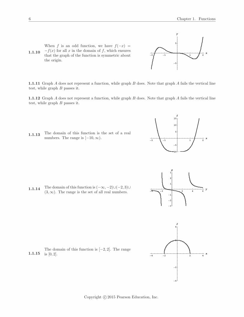
1.1.10
When f is an odd function, we have f(−x) =−f(x) for all x in the domain of f , which ensuresthat the graph of the function is symmetric aboutthe origin.
�2 �1 1 2x
�5
5
y
1.1.11 Graph A does not represent a function, while graph B does. Note that graph A fails the vertical linetest, while graph B passes it.
1.1.12 Graph A does not represent a function, while graph B does. Note that graph A fails the vertical linetest, while graph B passes it.
1.1.13 The domain of this function is the set of a realnumbers. The range is [−10,∞).
�2 �1 1 2x
�10
�5
5
10
15f
1.1.14 The domain of this function is (−∞,−2)∪(−2, 3)∪(3,∞). The range is the set of all real numbers. �4 �2 2 4 6
y
�3
�2
�1
1
2
3g
1.1.15The domain of this function is [−2, 2]. The rangeis [0, 2]. �4 �2 2 4
x
�4
�2
2
4f
Copyright c© 2015 Pearson Education, Inc.

1.1. Review of Functions 7
1.1.16 The domain of this function is (−∞, 2]. The rangeis [0,∞).
�3 �2 �1 0 1 2w
0.5
1.0
1.5
2.0F
1.1.17 The domain and the range for this function areboth the set of all real numbers. �5 5
u
�2
�1
1
2h
1.1.18 The domain of this function is [−5,∞). The rangeis approximately [−9.03,∞).
�4 �2 2 4 x
�10
10
20
30
40
50g
1.1.19 The domain of this function is [−3, 3]. The rangeis [0, 27].
�3 �2 �1 1 2 3 x
5
10
15
20
25
y
Copyright c© 2015 Pearson Education, Inc.

8 Chapter 1. Functions
1.1.20 The domain of this function is (−∞,∞)]. Therange is (0, 1].
�6 �4 �2 0 2 4 6 x
0.2
0.4
0.6
0.8
1.0
1.2
1.4
y
1.1.21 The independent variable t is elapsed time and the dependent variable d is distance above the ground.The domain in context is [0, 8]
1.1.22 The independent variable t is elapsed time and the dependent variable d is distance above the water.The domain in context is [0, 2]
1.1.23 The independent variable h is the height of the water in the tank and the dependent variable V isthe volume of water in the tank. The domain in context is [0, 50]
1.1.24 The independent variable r is the radius of the balloon and the dependent variable V is the volumeof the balloon. The domain in context is [0, 3
√3/(4π)]
1.1.25 f(10) = 96 1.1.26 f(p2) = (p2)2 − 4 = p4 − 4
1.1.27 g(1/z) = (1/z)3 = 1z3 1.1.28 F (y4) = 1
y4−3
1.1.29 F (g(y)) = F (y3) = 1y3−3 1.1.30 f(g(w)) = f(w3) = (w3)2 − 4 = w6 − 4
1.1.31 g(f(u)) = g(u2 − 4) = (u2 − 4)3
1.1.32 f(2+h)−f(2)h = (2+h)2−4−0
h = 4+4h+h2−4h = 4h+h2
h = 4 + h
1.1.33 F (F (x)) = F(
1x−3
)= 1
1x−3−3
= 11
x−3− 3(x−3)x−3
= 110−3xx−3
= x−310−3x
1.1.34 g(F (f(x))) = g(F (x2 − 4)) = g(
1x2−4−3
)=(
1x2−7
)31.1.35 f(
√x+ 4) = (
√x+ 4)2 − 4 = x+ 4− 4 = x.
1.1.36 F ((3x+ 1)/x) = 13x+1
x −3= 1
3x+1−3xx
= x3x+1−3x = x.
1.1.37 g(x) = x3 − 5 and f(x) = x10. The domain of h is the set of all real numbers.
1.1.38 g(x) = x6 + x2 + 1 and f(x) = 2x2 . The domain of h is the set of all real numbers.
1.1.39 g(x) = x4 + 2 and f(x) =√x. The domain of h is the set of all real numbers.
1.1.40 g(x) = x3 − 1 and f(x) = 1√x. The domain of h is the set of all real numbers for which x3 − 1 > 0,
which corresponds to the set (1,∞).
1.1.41 (f ◦g)(x) = f(g(x)) = f(x2−4) = |x2−4|. The domain of this function is the set of all real numbers.
1.1.42 (g ◦ f)(x) = g(f(x)) = g(|x|) = |x|2 − 4 = x2 − 4. The domain of this function is the set of all realnumbers.
Copyright c© 2015 Pearson Education, Inc.
1.1. Review of Functions 9
1.1.43 (f ◦G)(x) = f(G(x)) = f(
1x−2
)=∣∣∣ 1x−2
∣∣∣. The domain of this function is the set of all real numbers
except for the number 2.
1.1.44 (f ◦ g ◦G)(x) = f(g(G(x))) = f(g(
1x−2
))= f
((1
x−2
)2− 4
)=
∣∣∣∣( 1x−2
)2− 4
∣∣∣∣. The domain of this
function is the set of all real numbers except for the number 2.
1.1.45 (G ◦ g ◦ f)(x) = G(g(f(x))) = G(g(|x|)) = G(x2 − 4) = 1x2−4−2 = 1
x2−6 . The domain of this function
is the set of all real numbers except for the numbers ±√6.
1.1.46 (F ◦ g ◦ g)(x) = F (g(g(x))) = F (g(x2 − 4)) = F ((x2 − 4)2 − 4) =√(x2 − 4)2 − 4 =
√x4 − 8x2 + 12.
The domain of this function consists of the numbers x so that x4 − 8x2 + 12 ≥ 0. Because x4 − 8x2 + 12 =(x2 − 6) · (x2 − 2), we see that this expression is zero for x = ±√
6 and x = ±√2, By looking between these
points, we see that the expression is greater than or equal to zero for the set (−∞,−√6]∪[−√
2,√2]∪[√2,∞).
1.1.47 (g ◦ g)(x) = g(g(x)) = g(x2 − 4) = (x2 − 4)2 − 4 = x4 − 8x2 +16− 4 = x4 − 8x2 +12. The domain isthe set of all real numbers.
1.1.48 (G ◦G)(x) = G(G(x)) = G(1/(x− 2)) = 11
x−2−2= 1
1−2(x−2)x−2
= x−21−2x+4 = x−2
5−2x . Then G ◦G is defined
except where the denominator vanishes, so its domain is the set of all real numbers except for x = 52 .
1.1.49 Because (x2 + 3)− 3 = x2, we may choose f(x) = x− 3.
1.1.50 Because the reciprocal of x2 + 3 is 1x2+3 , we may choose f(x) = 1
x .
1.1.51 Because (x2 + 3)2 = x4 + 6x2 + 9, we may choose f(x) = x2.
1.1.52 Because (x2 + 3)2 = x4 + 6x2 + 9, and the given expression is 11 more than this, we may choosef(x) = x2 + 11.
1.1.53 Because (x2)2 + 3 = x4 + 3, this expression results from squaring x2 and adding 3 to it. Thus wemay choose f(x) = x2.
1.1.54 Because x2/3 + 3 = ( 3√x)2 + 3, we may choose f(x) = 3
√x.
1.1.55
a. (f ◦ g)(2) = f(g(2)) = f(2) = 4. b. g(f(2)) = g(4) = 1.
c. f(g(4)) = f(1) = 3. d. g(f(5)) = g(6) = 3.
e. f(f(8)) = f(8) = 8. f. g(f(g(5))) = g(f(2)) = g(4) = 1.
1.1.56
a. h(g(0)) = h(0) = −1. b. g(f(4)) = g(−1) = −1.
c. h(h(0)) = h(−1) = 0. d. g(h(f(4))) = g(h(−1)) = g(0) = 0.
e. f(f(f(1))) = f(f(0)) = f(1) = 0. f. h(h(h(0))) = h(h(−1)) = h(0) = −1.
g. f(h(g(2))) = f(h(3)) = f(0) = 1. h. g(f(h(4))) = g(f(4)) = g(−1) = −1.
i. g(g(g(1))) = g(g(2)) = g(3) = 4. j. f(f(h(3))) = f(f(0)) = f(1) = 0.
1.1.57 f(x+h)−f(x)h = (x+h)2−x2
h = (x2+2hx+h2)−x2
h = h(2x+h)h = 2x+ h.
1.1.58 f(x+h)−f(x)h = 4(x+h)−3−(4x−3)
h = 4x+4h−3−4x+3h = 4h
h = 4.
Copyright c© 2015 Pearson Education, Inc.
10 Chapter 1. Functions
1.1.59 f(x+h)−f(x)h =
2x+h− 2
x
h =2x−2(x+h)
x(x+h)
h = 2x−2x−2hhx(x+h) = − 2h
hx(x+h) = − 2x(x+h) .
1.1.60 f(x+h)−f(x)h = 2(x+h)2−3(x+h)+1−(2x2−3x+1)
h = 2x2+4xh+2h2−3x−3h+1−2x2+3x−1h =
4xh+2h2−3hh = h(4x+2h−3)
h = 4x+ 2h− 3.
1.1.61 f(x+h)−f(x)h =
x+hx+h+1− x
x+1
h =(x+h)(x+1)−x(x+h+1)
(x+1)(x+h+1)
h = x2+x+hx+h−x2−xh−xh(x+1)(x+h+1) =
hh(x+1)(x+h+1) =
1(x+1)(x+h+1)
1.1.62 f(x)−f(a)x−a = x4−a4
x−a = (x2−a2)(x2+a2)x−a = (x−a)(x+a)(x2+a2)
x−a = (x+ a)(x2 + a2).
1.1.63 f(x)−f(a)x−a = x3−2x−(a3−2a)
x−a = (x3−a3)−2(x−a)x−a = (x−a)(x2+ax+a2)−2(x−a)
x−a =(x−a)(x2+ax+a2−2)
x−a = x2 + ax+ a2 − 2.
1.1.64 f(x)−f(a)x−a = 4−4x−x2−(4−4a−a2)
x−a = −4(x−a)−(x2−a2)x−a = −4(x−a)−(x−a)(x+a)
x−a =(x−a)(−4−(x+a))
x−a = −4− x− a.
1.1.65 f(x)−f(a)x−a =
−4
x2 −−4
a2
x−a =−4a2+4x2
a2x2
x−a = 4(x2−a2)(x−a)a2x2 = 4(x−a)(x+a)
(x−a)a2x2 = 4(x+a)a2x2 .
1.1.66 f(x)−f(a)x−a =
1x−x2−( 1
a−a2)
x−a =1x− 1
a
x−a − x2−a2
x−a =a−xax
x−a − (x−a)(x+a)x−a = − 1
ax − (x+ a).
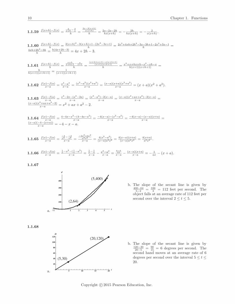
1.1.67
a.
�2,64�
�5,400�
�1 1 2 3 4 5 t
100
200
300
400
d
b. The slope of the secant line is given by400−645−2 = 336
3 = 112 feet per second. Theobject falls at an average rate of 112 feet persecond over the interval 2 ≤ t ≤ 5.
1.1.68
a.
�5,30�
�20,120�
5 10 15 20 t
20
40
60
80
100
120D
b. The slope of the secant line is given by120−3020−5 = 90
15 = 6 degrees per second. Thesecond hand moves at an average rate of 6degrees per second over the interval 5 ≤ t ≤20.
Copyright c© 2015 Pearson Education, Inc.

1.1. Review of Functions 11
1.1.69
a.
�1�2,4�
�2,1�
0.5 1.0 1.5 2.0 2.5 3.0 p
1
2
3
4
V
b. The slope of the secant line is given by1−4
2−(1/2) = − 33/2 = −2 cubic cm per atmo-
sphere. The volume decreases at an averagerate of 2 cubic cm per atmosphere over theinterval 0.5 ≤ p ≤ 2.
1.1.70
a.
�50,10 15 �
�150,30 5 �
20 40 60 80 100 120 140 l
10
20
30
40
50
60
S
b. The slope of the secant line is given by30
√5−10
√15
150−50 ≈ .2835 mph per foot. Thespeed of the car changes with an average rateof about .2835 mph per foot over the interval50 ≤ l ≤ 150.
1.1.71 This function is symmetric about the y-axis, because f(−x) = (−x)4+5(−x)2−12 = x4+5x2−12 =f(x).
1.1.72 This function is symmetric about the origin, because f(−x) = 3(−x)5 + 2(−x)3 − (−x) = −3x5 −2x3 + x = −(3x5 + 2x3 − x) = f(x).
1.1.73 This function has none of the indicated symmetries. For example, note that f(−2) = −26, whilef(2) = 22, so f is not symmetric about either the origin or about the y-axis, and is not symmetric aboutthe x-axis because it is a function.
1.1.74 This function is symmetric about the y-axis. Note that f(−x) = 2| − x| = 2|x| = f(x).
1.1.75 This curve (which is not a function) is symmetric about the x-axis, the y-axis, and the origin. Notethat replacing either x by −x or y by −y (or both) yields the same equation. This is due to the fact that(−x)2/3 = ((−x)2)1/3 = (x2)1/3 = x2/3, and a similar fact holds for the term involving y.
1.1.76 This function is symmetric about the origin. Writing the function as y = f(x) = x3/5, we see thatf(−x) = (−x)3/5 = −(x)3/5 = −f(x).
1.1.77 This function is symmetric about the origin. Note that f(−x) = (−x)|(−x)| = −x|x| = −f(x).
1.1.78 This curve (which is not a function) is symmetric about the x-axis, the y-axis, and the origin. Notethat replacing either x by −x or y by −y (or both) yields the same equation. This is due to the fact that| − x| = |x| and | − y| = |y|.
1.1.79 Function A is symmetric about the y-axis, so is even. Function B is symmetric about the origin, sois odd. Function C is also symmetric about the y-axis, so is even.
1.1.80 Function A is symmetric about the y-axis, so is even. Function B is symmetric about the origin, sois odd. Function C is also symmetric about the origin, so is odd.
Copyright c© 2015 Pearson Education, Inc.
12 Chapter 1. Functions
1.1.81
a. True. A real number z corresponds to the domain element z/2 + 19, because f(z/2 + 19) = 2(z/2 +19)− 38 = z + 38− 38 = z.
b. False. The definition of function does not require that each range element comes from a unique domainelement, rather that each domain element is paired with a unique range element.
c. True. f(1/x) = 11/x = x, and 1
f(x) =1
1/x = x.
d. False. For example, suppose that f is the straight line through the origin with slope 1, so that f(x) = x.Then f(f(x)) = f(x) = x, while (f(x))2 = x2.
e. False. For example, let f(x) = x+2 and g(x) = 2x−1. Then f(g(x)) = f(2x−1) = 2x−1+2 = 2x+1,while g(f(x)) = g(x+ 2) = 2(x+ 2)− 1 = 2x+ 3.
f. True. This is the definition of f ◦ g.g. True. If f is even, then f(−z) = f(z) for all z, so this is true in particular for z = ax. So if
g(x) = cf(ax), then g(−x) = cf(−ax) = cf(ax) = g(x), so g is even.
h. False. For example, f(x) = x is an odd function, but h(x) = x + 1 isn’t, because h(2) = 3, whileh(−2) = −1 which isn’t −h(2).
i. True. If f(−x) = −f(x) = f(x), then in particular −f(x) = f(x), so 0 = 2f(x), so f(x) = 0 for all x.
1.1.82
If n is odd, then n = 2k + 1 for some integer k,and (x)n = (x)2k+1 = x(x)2k, which is less than 0when x < 0 and greater than 0 when x > 0. Forany number P (positive or negative) the numbern√P is a real number when n is odd, and f( n
√P ) =
P . So the range of f in this case is the set of allreal numbers.If n is even, then n = 2k for some integer k, andxn = (x2)k. Thus g(−x) = g(x) = (x2)k ≥ 0 forall x. Also, for any nonnegative number M , wehave g( n
√M) = M , so the range of g in this case
is the set of all nonnegative numbers.
�4 �2 2 4x
�100
�50
50
100
f
�4 �2 2 4x
5
10
15
20
25
g
1.1.83
We will make heavy use of the fact that |x| is x ifx > 0, and is −x if x < 0. In the first quadrantwhere x and y are both positive, this equationbecomes x − y = 1 which is a straight line withslope 1 and y-intercept −1. In the second quad-rant where x is negative and y is positive, thisequation becomes −x− y = 1, which is a straightline with slope −1 and y-intercept −1. In the thirdquadrant where both x and y are negative, we ob-tain the equation −x − (−y) = 1, or y = x + 1,and in the fourth quadrant, we obtain x + y = 1.Graphing these lines and restricting them to theappropriate quadrants yields the following curve:
�4 �2 2 4x
�4
�2
2
4
y
Copyright c© 2015 Pearson Education, Inc.

1.1. Review of Functions 13
1.1.84
a. No. For example f(x) = x2 + 3 is an even function, but f(0) is not 0.
b. Yes. because f(−x) = −f(x), and because −0 = 0, we must have f(−0) = f(0) = −f(0), sof(0) = −f(0), and the only number which is its own additive inverse is 0, so f(0) = 0.
1.1.85 Because the composition of f with itself has first degree, f has first degree as well, so let f(x) = ax+b.Then (f ◦ f)(x) = f(ax+ b) = a(ax+ b) + b = a2x+ (ab+ b). Equating coefficients, we see that a2 = 9 andab+ b = −8. If a = 3, we get that b = −2, while if a = −3 we have b = 4. So the two possible answers aref(x) = 3x− 2 and f(x) = −3x+ 4.
1.1.86 Since the square of a linear function is a quadratic, we let f(x) = ax+b. Then f(x)2 = a2x2+2abx+b2.Equating coefficients yields that a = ±3 and b = ±2. However, a quick check shows that the middle termis correct only when one of these is positive and one is negative. So the two possible such functions f aref(x) = 3x− 2 and f(x) = −3x+ 2.
1.1.87 Let f(x) = ax2 + bx+ c. Then (f ◦ f)(x) = f(ax2 + bx+ c) = a(ax2 + bx+ c)2 + b(ax2 + bx+ c) + c.Expanding this expression yields a3x4 +2a2bx3 +2a2cx2 + ab2x2 +2abcx+ ac2 + abx2 + b2x+ bc+ c, whichsimplifies to a3x4 +2a2bx3 + (2a2c+ ab2 + ab)x2 + (2abc+ b2)x+ (ac2 + bc+ c). Equating coefficients yieldsa3 = 1, so a = 1. Then 2a2b = 0, so b = 0. It then follows that c = −6, so the original function wasf(x) = x2 − 6.
1.1.88 Because the square of a quadratic is a quartic, we let f(x) = ax2 + bx + c. Then the square of fis c2 + 2bcx + b2x2 + 2acx2 + 2abx3 + a2x4. By equating coefficients, we see that a2 = 1 and so a = ±1.Because the coefficient on x3 must be 0, we have that b = 0. And the constant term reveals that c = ±6. Aquick check shows that the only possible solutions are thus f(x) = x2 − 6 and f(x) = −x2 + 6.
1.1.89 f(x+h)−f(x)h =
√x+h−√
xh =
√x+h−√
xh ·
√x+h+
√x√
x+h+√x= (x+h)−x
h(√x+h+
√x)
= 1√x+h+
√x.
f(x)−f(a)x−a =
√x−√
ax−a =
√x−√
ax−a ·
√x+
√a√
x+√a= x−a
(x−a)(√x+
√a)
= 1√x+
√a.
1.1.90 f(x+h)−f(x)h =
√1−2(x+h)−√
1−2x
h =
√1−2(x+h)−√
1−2x
h ·√
1−2(x+h)+√1−2x√
1−2(x+h)+√1−2x
=
1−2(x+h)−(1−2x)
h(√
1−2(x+h)+√1−2x)
= − 2√1−2(x+h)+
√1−2x
.
f(x)−f(a)x−a =
√1−2x−√
1−2ax−a =
√1−2x−√
1−2ax−a ·
√1−2x+
√1−2a√
1−2x+√1−2a
= (1−2x)−(1−2a)
(x−a)(√1−2x+
√1−2a)
=(−2)(x−a)
(x−a)(√1−2x+
√1−2a)
= − 2(√1−2x+
√1−2a)
.
1.1.91 f(x+h)−f(x)h =
−3√x+h
− −3√x
h = −3(√x−√
x+h)
h√x√x+h
= −3(√x−√
x+h)
h√x√x+h
·√x+
√x+h√
x+√x+h
=−3(x−(x+h))
h√x√x+h(
√x+
√x+h)
= 3√x√x+h(
√x+
√x+h)
.
f(x)−f(a)x−a =
−3√x−−3√
a
x−a =−3
(√a−√
x√a√
x
)x−a = (−3)(
√a−√
x)(x−a)
√a√x
·√a+
√x√
a+√x= (3)(x−a)
(x−a)(√a√x)(
√a+
√x)
= 3√ax(
√a+
√x).
1.1.92 f(x+h)−f(x)h =
√(x+h)2+1−√
x2+1
h =
√(x+h)2+1−√
x2+1
h ·√
(x+h)2+1+√x2+1√
(x+h)2+1+√x2+1
=
(x+h)2+1−(x2+1)
h(√
(x+h)2+1+√x2+1)
= x2+2hx+h2−x2
h(√
(x+h)2+1+√x2+1)
= 2x+h√(x+h)2+1+
√x2+1
.
f(x)−f(a)x−a =
√x2+1−√
a2+1x−a =
√x2+1−√
a2+1x−a ·
√x2+1+
√a2+1√
x2+1+√a2+1
= x2+1−(a2+1)
(x−a)(√x2+1+
√a2+1)
=
(x−a)(x+a)
(x−a)(√x2+1+
√a2+1)
= x+a√x2+1+
√a2+1
.
Copyright c© 2015 Pearson Education, Inc.

14 Chapter 1. Functions
1.1.93
a. The formula for the height of the rocket isvalid from t = 0 until the rocket hits theground, which is the positive solution to−16t2 + 96t+ 80 = 0, which the quadraticformula reveals is t = 3 +
√14. Thus, the
domain is [0, 3 +√14]. b. 1 2 3 4 5 6
t
50
100
150
200
h
The maximum appears to occur at t = 3.The height at that time would be 224.
1.1.94
a. d(0) = (10− (2.2) · 0)2 = 100.
b. The tank is first empty when d(t) = 0, which is when 10− (2.2)t = 0, or t = 50/11.
c. An appropriate domain would [0, 50/11].
1.1.95 This would not necessarily have either kind of symmetry. For example, f(x) = x2 is an even functionand g(x) = x3 is odd, but the sum of these two is neither even nor odd.
1.1.96 This would be an odd function, so it would be symmetric about the origin. Suppose f is even and gis odd. Then (f · g)(−x) = f(−x)g(−x) = f(x) · (−g(x)) = −(f · g)(x).1.1.97 This would be an odd function, so it would be symmetric about the origin. Suppose f is even and g
is odd. Then fg (−x) = f(−x)
g(−x) = f(x)−g(x) = − f
g (x).
1.1.98 This would be an even function, so it would be symmetric about the y-axis. Suppose f is even andg is odd. Then f(g(−x)) = f(−g(x)) = f(g(x)).
1.1.99 This would be an even function, so it would be symmetric about the y-axis. Suppose f is even andg is even. Then f(g(−x)) = f(g(x)), because g(−x) = g(x).
1.1.100 This would be an odd function, so it would be symmetric about the origin. Suppose f is odd andg is odd. Then f(g(−x)) = f(−g(x)) = −f(g(x)).
1.1.101 This would be an even function, so it would be symmetric about the y-axis. Suppose f is even andg is odd. Then g(f(−x)) = g(f(x)), because f(−x) = f(x).
1.1.102
a. f(g(−1)) = f(−g(1)) = f(3) = 3 b. g(f(−4)) = g(f(4)) = g(−4) = −g(4) = 2
c. f(g(−3)) = f(−g(3)) = f(4) = −4 d. f(g(−2)) = f(−g(2)) = f(1) = 2
e. g(g(−1)) = g(−g(1)) = g(3) = −4 f. f(g(0)− 1) = f(−1) = f(1) = 2
g. f(g(g(−2))) = f(g(−g(2))) = f(g(1)) = f(−3) = 3 h. g(f(f(−4))) = g(f(−4)) = g(−4) = 2
i. g(g(g(−1))) = g(g(−g(1))) = g(g(3)) = g(−4) = 2
1.1.103
a. f(g(−2)) = f(−g(2)) = f(−2) = 4 b. g(f(−2)) = g(f(2)) = g(4) = 1
c. f(g(−4)) = f(−g(4)) = f(−1) = 3 d. g(f(5)− 8) = g(−2) = −g(2) = −2
e. g(g(−7)) = g(−g(7)) = g(−4) = −1 f. f(1− f(8)) = f(−7) = 7
Copyright c© 2015 Pearson Education, Inc.

1.2. Representing Functions 15
1.2 Representing Functions
1.2.1 Functions can be defined and represented by a formula, through a graph, via a table, and by usingwords.
1.2.2 The domain of every polynomial is the set of all real numbers.
1.2.3 The domain of a rational function p(x)q(x) is the set of all real numbers for which q(x) = 0.
1.2.4 A piecewise linear function is one which is linear over intervals in the domain.
1.2.5
�2 �1 1 2x
�15
�10
�5
5
10
15y
1.2.6
�2 �1 1 2x
�1.0
�0.5
0.5
1.0
y
1.2.7 Compared to the graph of f(x), the graph of f(x+ 2) will be shifted 2 units to the left.
1.2.8 Compared to the graph of f(x), the graph of −3f(x) will be scaled vertically by a factor of 3 andflipped about the x axis.
1.2.9 Compared to the graph of f(x), the graph of f(3x) will be scaled horizontally by a factor of 3.
1.2.10 To produce the graph of y = 4(x+ 3)2 + 6 from the graph of x2, one must
1. shift the graph horizontally by 3 units to left
2. scale the graph vertically by a factor of 4
3. shift the graph vertically up 6 units.
1.2.11 The slope of the line shown is m = −3−(−1)3−0 = −2/3. The y-intercept is b = −1. Thus the function
is given by f(x) = (−2/3)x− 1.
1.2.12 The slope of the line shown is m = 1−(5)5−0 = −4/5. The y-intercept is b = 5. Thus the function is
given by f(x) = (−4/5)x+ 5.
1.2.13
The slope is given by 5−32−1 = 2, so the equation of
the line is y − 3 = 2(x− 1), which can be writtenas y = 2x− 2 + 3, or y = 2x+ 1.
�2 �1 1 2 x
�2
2
4
y
Copyright c© 2015 Pearson Education, Inc.

16 Chapter 1. Functions
1.2.14
The slope is given by 0−(−3)5−2 = 1, so the equation
of the line is y − 0 = 1(x− 5), or y = x− 5. 2 4 6 8 10 x
�4
�2
2
4
y
1.2.15 Using price as the independent variable p and the average number of units sold per day as thedependent variable d, we have the ordered pairs (250, 12) and (200, 15). The slope of the line determined bythese points is m = 15−12
200−250 = − 350 . Thus the demand function has the form d(p) = (−3/50)p+ b for some
constant b. Using the point (200, 15), we find that 15 = (−3/50) · 200 + b, so b = 27. Thus the demandfunction is d = (−3/50)p + 27. While the domain of this linear function is the set of all real numbers, theformula is only likely to be valid for some subset of the interval (0, 450), because outside of that intervaleither p ≤ 0 or d ≤ 0.
100 200 300 400 p
5
10
15
20
25
d
1.2.16 The profit is given by p = f(n) = 8n− 175. The break-even point is when p = 0, which occurs whenn = 175/8 = 21.875, so they need to sell at least 22 tickets to not have a negative profit.
10 20 30 40 50 n
�100
100
200
p
1.2.17 The slope is given by the rate of growth, which is 24. When t = 0 (years past 2015), the populationis 500, so the point (0, 500) satisfies our linear function. Thus the population is given by p(t) = 24t + 500.In 2030, we have t = 15, so the population will be approximately p(15) = 360 + 500 = 860.
5 10 15 20 t
200
400
600
800
1000p
Copyright c© 2015 Pearson Education, Inc.

1.2. Representing Functions 17
1.2.18 The cost per mile is the slope of the desired line, and the intercept is the fixed cost of 3.5. Thus, thecost per mile is given by c(m) = 2.5m+ 3.5. When m = 9, we have c(9) = (2.5)(9) + 3.5 = 22.5 + 3.5 = 26dollars.
2 4 6 8 10 12 14 m
10
20
30
40
c
1.2.19 For x < 0, the graph is a line with slope 1 and y- intercept 3, while for x > 0, it is a line with slope−1/2 and y-intercept 3. Note that both of these lines contain the point (0, 3). The function shown can thusbe written
f(x) =
⎧⎨⎩x+ 3 if x < 0;
− 12x+ 3 if x ≥ 0.
1.2.20 For x < 3, the graph is a line with slope 1 and y- intercept 1, while for x > 3, it is a line with slope−1/3. The portion to the right thus is represented by y = (−1/3)x + b, but because it contains the point(6, 1), we must have 1 = (−1/3)(6) + b so b = 3. The function shown can thus be written
f(x) =
⎧⎨⎩x+ 1 if x < 3;
− 13x+ 3 if x ≥ 3.
Note that at x = 3 the value of the function is 2, as indicated by our formula.
1.2.21
The cost is given by
c(t) =
⎧⎨⎩0.05t for 0 ≤ t ≤ 60
1.2 + 0.03t for 60 < t ≤ 120.
20 40 60 80 100 120 t
1
2
3
4
y
1.2.22
The cost is given by
c(m) =
⎧⎨⎩3.5 + 2.5m for 0 ≤ m ≤ 5
8.5 + 1.5m for m > 5.
2 4 6 8 10 m
5
10
15
20
y
Copyright c© 2015 Pearson Education, Inc.

18 Chapter 1. Functions
1.2.23
1 2 3 4 x
1
2
3
4y
1.2.24
1 2 3 4 x
2
3
4
5y
1.2.25
�2 �1 1 2 x
�6
�4
�2
y
1.2.26
0.5 1.0 1.5 2.0 x
�1
1
2
3y
1.2.27
�2 �1 0 1 2 x
0.5
1.0
1.5
2.0
2.5
3.0y
1.2.28
�1 1 2 3 4 x
1
2
3
4y
1.2.29
a.
�2 �1 1 2 3 x
5
10
15y
b. The function is a polynomial, so its domain is the setof all real numbers.
c. It has one peak near its y-intercept of (0, 6) and onevalley between x = 1 and x = 2. Its x-intercept isnear x = −4/3.
Copyright c© 2015 Pearson Education, Inc.

1.2. Representing Functions 19
1.2.30
a.
�6 �4 �2 2 4 6x
�2
�1
1
2
3
4y
b. The function’s domain is the set of all real numbers.
c. It has a valley at the y-intercept of (0,−2), and is verysteep at x = −2 and x = 2 which are the x-intercepts.It is symmetric about the y-axis.
1.2.31
a. �8 �6 �4 �2 2 4 6x
5
10
15
20
25
y
b. The domain of the function is the set of all real num-bers except −3.
c. There is a valley near x = −5.2 and a peak nearx = −0.8. The x-intercepts are at −2 and 2, wherethe curve does not appear to be smooth. There is avertical asymptote at x = −3. The function is neverbelow the x-axis. The y-intercept is (0, 4/3).
1.2.32
a.
�15 �10 �5 5 10 15x
�2.0
�1.5
�1.0
�0.5
0.5
1.0
1.5
y
b. The domain of the function is (−∞,−2] ∪ [2,∞)
c. x-intercepts are at −2 and 2. Because 0 isn’t in thedomain, there is no y-intercept. The function has avalley at x = −4.
1.2.33
a.
�3 �2 �1 1 2 3 4 x
�4
�3
�2
�1
1
2
3y
b. The domain of the function is (−∞,∞)
c. The function has a maximum of 3 at x = 1/2, and ay-intercept of 2.
Copyright c© 2015 Pearson Education, Inc.

20 Chapter 1. Functions
1.2.34
a.
�1 1 2 3 x
�1.5
�1.0
�0.5
0.5
1.0
1.5y
b. The domain of the function is (−∞,∞)
c. The function contains a jump at x = 1. The max-imum value of the function is 1 and the minimumvalue is −1.
1.2.35 The slope of this line is constantly 2, so the slope function is s(x) = 2.
1.2.36 The function can be written as |x| =⎧⎨⎩−x if x ≤ 0
x if x > 0.
The slope function is s(x) =
⎧⎨⎩−1 if x < 0
1 if x > 0.
1.2.37 The slope function is given by s(x) =
⎧⎨⎩1 if x < 0;
−1/2 if x > 0.
1.2.38 The slope function is given by s(x) =
⎧⎨⎩1 if x < 3;
−1/3 if x > 3.
1.2.39
a. Because the area under consideration is that of a rectangle with base 2 and height 6, A(2) = 12.
b. Because the area under consideration is that of a rectangle with base 6 and height 6, A(6) = 36.
c. Because the area under consideration is that of a rectangle with base x and height 6, A(x) = 6x.
1.2.40
a. Because the area under consideration is that of a triangle with base 2 and height 1, A(2) = 1.
b. Because the area under consideration is that of a triangle with base 6 and height 3, the A(6) = 9.
c. Because A(x) represents the area of a triangle with base x and height (1/2)x, the formula for A(x) is12 · x · x
2 = x2
4 .
1.2.41
a. Because the area under consideration is that of a trapezoid with base 2 and heights 8 and 4, we haveA(2) = 2 · 8+4
2 = 12.
b. Note that A(3) represents the area of a trapezoid with base 3 and heights 8 and 2, so A(3) = 3· 8+22 = 15.
So A(6) = 15+(A(6)−A(3)), and A(6)−A(3) represents the area of a triangle with base 3 and height2. Thus A(6) = 15 + 6 = 21.
Copyright c© 2015 Pearson Education, Inc.

1.2. Representing Functions 21
c. For x between 0 and 3, A(x) represents the area of a trapezoid with base x, and heights 8 and 8− 2x.Thus the area is x · 8+8−2x
2 = 8x−x2. For x > 3, A(x) = A(3)+A(x)−A(3) = 15+2(x− 3) = 2x+9.Thus
A(x) =
⎧⎨⎩8x− x2 if 0 ≤ x ≤ 3;
2x+ 9 if x > 3.
1.2.42
a. Because the area under consideration is that of trapezoid with base 2 and heights 3 and 1, we haveA(2) = 2 · 3+1
2 = 4.
b. Note that A(6) = A(2)+(A(6)−A(2), and that A(6)−A(2) represents a trapezoid with base 6−2 = 4and heights 1 and 5. The area is thus 4 +
(4 · 1+5
2
)= 4 + 12 = 16.
c. For x between 0 and 2, A(x) represents the area of a trapezoid with base x, and heights 3 and 3− x.
Thus the area is x · 3+3−x2 = 3x− x2
2 . For x > 2, A(x) = A(2)+A(x)−A(2) = 4+(A(x)−A(2)). Notethat A(x) − A(2) represents the area of a trapezoid with base x − 2 and heights 1 and x − 1. Thus
A(x) = 4 + (x− 2) · 1+x−12 = 4 + (x− 2)
(x2
)= x2
2 − x+ 4. Thus
A(x) =
⎧⎨⎩3x− x2
2 if 0 ≤ x ≤ 2;
x2
2 − x+ 4 if x > 2.
1.2.43 f(x) = |x− 2|+3, because the graph of f is obtained from that of |x| by shifting 2 units to the rightand 3 units up.
g(x) = −|x + 2| − 1, because the graph of g is obtained from the graph of |x| by shifting 2 units to theleft, then reflecting about the x-axis, and then shifting 1 unit down.
1.2.44
a.
�4 �2 2 4x
�4
�2
2
4y
b. �4 �3 �2 �1 0 1 2x
1
2
3
4y
c. �2 �1 0 1 2 3 4x
1
2
3
4y
d. �4 �2 0 2 4x
2
4
6
8y
e. �4 �2 0 2 4x
2
4
6
8y
f. �4 �2 0 2 4x
2
4
6
8y
Copyright c© 2015 Pearson Education, Inc.

22 Chapter 1. Functions
1.2.45
a. Shift 3 units to the right.
�1 0 1 2 3 4 5x
2
4
6
8y
b. Horizontal scaling by a factor of 2, then shift 2 units to the right.
�1 0 1 2 3 4 5x
2
4
6
8y
c. Shift to the right 2 units, vertical scaling by a factor of 3 and flip, shift up 4 units.
�1 1 2 3 4 5x
�4
�2
2
4y
d. Horizontal scaling by a factor of 13 , horizontal shift right 2 units, vertical scaling by a factor of 6,
vertical shift up 1 unit.
�1 1 2 3 4 5x
�4
�2
2
4y
1.2.46
a. Shift 4 units to the left.
Copyright c© 2015 Pearson Education, Inc.

1.2. Representing Functions 23
�4 �3 �2 �1 0 1 2 3x
1
2
3
4y
b. Horizontal scaling by a factor of 2, shift 12 unit to the right, vertical scaling by a factor of 2.
�1 0 1 2 3 4 5 6x
1
2
3
4
5
6y
c. Shift 1 unit to the right.
0 1 2 3 4 5x
0.5
1.0
1.5
2.0
2.5
3.0y
d. Shift 1 unit to the right, vertical scaling by a factor of 3, vertical shift down 5 units.
1 2 3 4 5 6 7x
�5
�4
�3
�2
�1
1
2y
1.2.47The graph is obtained by shifting the graph of x2
two units to the right and one unit up.
�1 1 2 3 4 5 x
2
4
6
8
10y
Copyright c© 2015 Pearson Education, Inc.

24 Chapter 1. Functions
1.2.48
Write x2−2x+3 as (x2−2x+1)+2 = (x−1)2+2.The graph is obtained by shifting the graph of x2
one unit to the right and two units up.
�2 2 4 x
5
10
15
y
1.2.49This function is −3f(x) where f(x) = x2. Verti-cally scale the graph of f by a factor of 3 and thenflip.
�2 �1 1 2x
�12
�10
�8
�6
�4
�2
y
1.2.50This function is 2f(x) − 1 where f(x) = x3. Ver-tically scale the graph of f by a factor of 2 andthen vertically shift down 1 unit.
�1.5 �1.0 �0.5 0.5 1.0 1.5x
�8
�6
�4
�2
2
4
6y
1.2.51This function is 2f(x + 3) where f(x) = x2. Ver-tically scale the graph of f by a factor of 2 andthen shift left 3 units.
�6 �4 �2x
5
10
15
20
25
30
y
1.2.52
By completing the square, we have that p(x) =(x2+3x+(9/4))− (29/4) = (x+(3/2))2− (29/4).So it is f(x + (3/2)) − (29/4) where f(x) = x2.Shift the graph of f 3/2 units to the left and thendown 29/4 units.
�4 �3 �2 �1 1 2x
�6
�4
�2
2
4
y
Copyright c© 2015 Pearson Education, Inc.

1.2. Representing Functions 25
1.2.53
By completing the square, we have that h(x) =−4(x2 + x − 3) = −4
(x2 + x+ 1
4 − 14 − 3
)=
−4(x+ (1/2))2 + 13. So it is −4f(x+ (1/2)) + 13where f(x) = x2. Vertically scale the graph of fby a factor of 4, then reflect about the x-axis, thenshift left 1/2 unit, and then up 13 units.
�3 �2 �1 1 2 3x
�30
�20
�10
10
y
1.2.54
Because |3x−6|+1 = 3|x−2|+1, this is 3f(x−2)+1where f(x) = |x|. Shift the graph of f 2 units tothe right, vertically scale by a factor of 3, and thenshift 1 unit up.
�1 0 1 2 3 4x
2
4
6
8y
1.2.55
a. True. A polynomial p(x) can be written as the ratio of polynomials p(x)1 , so it is a rational function.
However, a rational function like 1x is not a polynomial.
b. False. For example, if f(x) = 2x, then (f ◦ f)(x) = f(f(x)) = f(2x) = 4x is linear, not quadratic.
c. True. In fact, if f is degree m and g is degree n, then the degree of the composition of f and g is m ·n,regardless of the order they are composed.
d. False. The graph would be shifted two units to the left.
1.2.56 The points of intersection are found by solving x2 + 2 = x + 4. This yields the quadratic equationx2 − x− 2 = 0 or (x− 2)(x+ 1) = 0. So the x-values of the points of intersection are 2 and −1. The actualpoints of intersection are (2, 6) and (−1, 3).
1.2.57 The points of intersection are found by solving x2 = −x2 + 8x. This yields the quadratic equation2x2 − 8x = 0 or (2x)(x− 4) = 0. So the x-values of the points of intersection are 0 and 4. The actual pointsof intersection are (0, 0) and (4, 16).
1.2.58 y = x+ 1, because the y value is always 1 more than the x value.
1.2.59 y =√x− 1, because the y value is always 1 less than the square root of the x value.
1.2.60 y = x3 − 1. The domain is (−∞,∞). �2 �1 1 2x
�5
5
y
Copyright c© 2015 Pearson Education, Inc.

26 Chapter 1. Functions
1.2.61
The car moving north has gone 30t miles aftert hours and the car moving east has gone 60tmiles. Using the Pythagorean theorem, we haves(t) =
√(30t)2 + (60t)2 =
√900t2 + 3600t2 =√
4500t2 = 30√5t miles. The context domain
could be [0, 4].1 2 3 4
s
50
100
150
200
250
t
1.2.62y = 50
x . Theoretically the domain is (0,∞), butthe world record for the “hour ride” is just shortof 50 miles.
10 20 30 40 50x
2
4
6
8
10
12
y
1.2.63
y = 3200x . Note that x dollars per gallon
32 miles per gallon · ymileswould represent the numbers of dollars, so thismust be 100. So we have xy
32 = 100, or y = 3200x .
We certainly have x > 0, and a reasonable upperbound to imagine for x is $5 (let’s hope), so thecontext domain is (0, 5].
0 1 2 3 4 5 x : dollars
1000
2000
3000
4000
5000
6000
7000y : miles
1.2.64
�3 �2 �1 1 2 3x
�3
�2
�1
1
2y
1.2.65
�3 �2 �1 1 2 3x
�2
�1
1
2
3y
Copyright c© 2015 Pearson Education, Inc.

1.2. Representing Functions 27
1.2.66
�1 0 1 2 3x
0.2
0.4
0.6
0.8
y
1.2.67
�1 1 2 3x
0.2
0.4
0.6
0.8
1.0y
1.2.68
�2 �1 1 2x
20
40
60
80
y
1.2.69
�2 �1 1 2 x
�2
�1
1
2
y
1.2.70
1 2 3 4 5x
0.5
1.0
1.5
2.0
y
1.2.71
a. The zeros of f are the points where the graph crosses the x-axis, so these are points A, D, F , and I.
b. The only high point, or peak, of f occurs at point E, because it appears that the graph has larger andlarger y values as x increases past point I and decreases past point A.
c. The only low points, or valleys, of f are at points B and H, again assuming that the graph of fcontinues its apparent behavior for larger values of x.
d. Past point H, the graph is rising, and is rising faster and faster as x increases. It is also rising betweenpoints B and E, but not as quickly as it is past point H. So the marked point at which it is risingmost rapidly is I.
e. Before point B, the graph is falling, and falls more and more rapidly as x becomes more and morenegative. It is also falling between points E and H, but not as rapidly as it is before point B. So themarked point at which it is falling most rapidly is A.
1.2.72
a. The zeros of g appear to be at x = 0, x = 1, x = 1.6, and x ≈ 3.15.
b. The two peaks of g appear to be at x ≈ 0.5 and x ≈ 2.6, with corresponding points ≈ (0.5, 0.4) and≈ (2.6, 3.4).
Copyright c© 2015 Pearson Education, Inc.
28 Chapter 1. Functions
c. The only valley of g is at ≈ (1.3,−0.2).
d. Moving right from x ≈ 1.3, the graph is rising more and more rapidly until about x = 2, at whichpoint it starts rising less rapidly (because, by x ≈ 2.6, it is not rising at all). So the coordinates of thepoint at which it is rising most rapidly are approximately (2.1, g(2)) ≈ (2.1, 2). Note that while thecurve is also rising between x = 0 and x ≈ 0.5, it is not rising as rapidly as it is near x = 2.
e. To the right of x ≈ 2.6, the curve is falling, and falling more and more rapidly as x increases. So thepoint at which it is falling most rapidly in the interval [0, 3] is at x = 3, which has the approximatecoordinates (3, 1.4). Note that while the curve is also falling between x ≈ 0.5 and x ≈ 1.3, it is notfalling as rapidly as it is near x = 3.
1.2.73
a. �15 �10 �5 5 10 15 �
0.2
0.4
0.6
0.8
1.0y
b. This appears to have a maximum when θ = 0. Ourvision is sharpest when we look straight ahead.
c. For |θ| ≤ .19◦. We have an extremely narrowrange where our eyesight is sharp.
1.2.74
a. f(.75) = .752
1−2(.75)(.25) = .9. There is a 90% chance that the server will win from deuce if they win 75%
of their service points.
b. f(.25) = .252
1−2(.25)(.75) = .1. There is a 10% chance that the server will win from deuce if they win 25%
of their service points.
1.2.75
a. Using the points (1986, 1875) and (2000, 6471) we see that the slope is about 328.3. At t = 0, the valueof p is 1875. Therefore a line which reasonably approximates the data is p(t) = 328.3t+ 1875.
b. Using this line, we have that p(9) = 4830.
1.2.76
a. We know that the points (32, 0) and (212, 100) are on our line. The slope of our line is thus 100−0212−32 =
100180 = 5
9 . The function f(F ) thus has the form C = (5/9)F + b, and using the point (32, 0) we see that0 = (5/9)32 + b, so b = −(160/9). Thus C = (5/9)F − (160/9)
b. Solving the system of equations C = (5/9)F −(160/9) and C = F , we have that F = (5/9)F −(160/9),so (4/9)F = −160/9, so F = −40 when C = −40.
1.2.77
a. Because you are paying $350 per month, the amount paid after m months is y = 350m+ 1200.
b. After 4 years (48 months) you have paid 350 · 48 + 1200 = 18000 dollars. If you then buy the car for$10,000, you will have paid a total of $28,000 for the car instead of $25,000. So you should buy thecar instead of leasing it.
Copyright c© 2015 Pearson Education, Inc.

1.2. Representing Functions 29
1.2.78
Because S = 4πr2, we have that r2 = S4π , so |r| =√
S2√π, but because r is positive, we can write r =
√S
2√π.
2 4 6 8S
0.2
0.4
0.6
0.8
r
1.2.79 The function makes sense for 0 ≤ h ≤ 2.
0.5 1.0 1.5 2.0h
1
2
3
4
V
1.2.80
a. Note that the island, the point P on shore, andthe point down shore x units from P form a righttriangle. By the Pythagorean theorem, the lengthof the hypotenuse is
√40000 + x2. So Kelly must
row this distance and then jog 600−xmeters to gethome. So her total distance d(x) =
√40000 + x2+
(600− x). 100 200 300 400 500 600x
200
400
600
800d
b. Because distance is rate times time, we have thattime is distance divided by rate. Thus T (x) =√
40000+x2
2 + 600−x4 .
100 200 300 400 500 600x
50
100
150
200
250
300
T
c. By inspection, it looks as though she should head to a point about 115 meters down shore from P .This would lead to a time of about 236.6 seconds.
1.2.81
a. The volume of the box is x2h, but because the boxhas volume 125 cubic feet, we have that x2h = 125,so h = 125
x2 . The surface area of the box is givenby x2 (the area of the base) plus 4 · hx, becauseeach side has area hx. Thus S = x2 + 4hx =x2 + 4·125·x
x2 = x2 + 500x .
0 5 10 15 20x
100
200
300
400
500y
b. By inspection, it looks like the value of x which minimizes the surface area is about 6.3.
1.2.82 Let f(x) = anxn + smaller degree terms and let g(x) = bmxm + some smaller degree terms.
Copyright c© 2015 Pearson Education, Inc.

30 Chapter 1. Functions
a. The largest degree term in f ·f is anxn ·anxn = a2nx
n+n, so the degree of this polynomial is n+n = 2n.
b. The largest degree term in f ◦ f is an · (anxn)n, so the degree is n2.
c. The largest degree term in f · g is anbmxm+n, so the degree of the product is m+ n.
d. The largest degree term in f ◦ g is an · (bmxm)n, so the degree is mn.
1.2.83 Suppose that the parabola f crosses the x-axis at a and b, with a < b. Then a and b are roots of thepolynomial, so (x− a) and (x− b) are factors. Thus the polynomial must be f(x) = c(x− a)(x− b) for somenon-zero real number c. So f(x) = cx2 − c(a + b)x + abc. Because the vertex always occurs at the x value
which is −coefficient on x2·coefficient on x2 we have that the vertex occurs at c(a+b)
2c = a+b2 , which is halfway between a and b.
1.2.84
a. We complete the square to rewrite the function f . Write f(x) = ax2+ bx+ c as f(x) = a(x2+ bax+
ca ).
Completing the square yields
a
((x2 +
b
ax+
b2
4a
)+
(c
a− b2
4a
))= a
(x+
b
2a
)2
+
(c− b2
4
).
Thus the graph of f is obtained from the graph of x2 by shifting b2a units to the left (and then
doing some scaling and vertical shifting) – moving the vertex from 0 to − b2a . The vertex is therefore(
−b2a , c− b2
4
).
b. We know that the graph of f touches the x-axis twice if the equation ax2 + bx + c = 0 has two realsolutions. By the quadratic formula, we know that this occurs exactly when the discriminant b2 − 4acis positive. So the condition we seek is for b2 − 4ac > 0, or b2 > 4ac.
1.2.85
a.n 1 2 3 4 5
n! 1 2 6 24 120
b.
1 2 3 4 5n
20
40
60
80
100
120
c. Using trial and error and a calculator yields that 10! is more than a million, but 9! isn’t.
1.2.86
a.n 1 2 3 4 5 6 7 8 9 10
S(n) 1 3 6 10 15 21 28 36 45 55
b. The domain of this function consists of the positive integers. The range is a subset of the set of positiveintegers.
c. Using trial and error and a calculator yields that S(n) > 1000 for the first time for n = 45.
1.2.87
a.n 1 2 3 4 5 6 7 8 9 10
T (n) 1 5 14 30 55 91 140 204 285 385
b. The domain of this function consists of the positive integers.
c. Using trial and error and a calculator yields that T (n) > 1000 for the first time for n = 14.
Copyright c© 2015 Pearson Education, Inc.
1.3. Trigonometric Functions 31
1.3 Trigonometric Functions
1.3.1 Let O be the length of the side opposite the angle x, let A be length of the side adjacent to the anglex, and let H be the length of the hypotenuse. Then sinx = O
H , cosx = AH , tanx = O
A , cscx = HO , secx = H
A ,
and cotx = AO .
1.3.2 We consider the angle formed by the positive x axis and the ray from the origin through the pointP (x, y). A positive angle is one for which the rotation from the positive x axis to the other ray is counter-
clockwise. We then define the six trigonometric functions as follows: let r =√
x2 + y2. Then sin θ = yr ,
cos θ = xr , tan θ = y
x , csc θ = ry , sec θ = r
x , and cot θ = xy .
1.3.3 The radian measure of an angle θ is the length of the arc s on the unit circle associated with θ.
1.3.4 The period of a function is the smallest positive real number k so that f(x + k) = f(x) for all x inthe domain of the function. The sine, cosine, secant, and cosecant function all have period 2π. The tangentand cotangent functions have period π.
1.3.5 sin2 x+ cos2 x = 1, 1 + cot2 x = csc2 x, and tan2 x+ 1 = sec2 x.
1.3.6 cscx = 1sin x , secx = 1
cos x , tanx = sin xcos x , and cotx = cos x
sin x .
1.3.7 The tangent function is undefined where cosx = 0, which is at all real numbers of the form π2 +
kπ, k an integer. This is the set of odd multiples of π/2.
1.3.8 secx is defined wherever cosx = 0, which is {x : x = π2 + kπ, k an integer}. This is the set of odd
multiples of π/2.
1.3.9
The point on the unit circle associated with 2π/3is (−1/2,
√3/2), so cos(2π/3) = −1/2.
��1
2,
3
2�
�1.0 �0.5 0.5 1.0
�1.0
�0.5
0.5
1.0
1.3.10 The point on the unit circle associated with 2π/3 is (−1/2,√3/2), so sin(2π/3) =
√3/2. See the
picture from the previous problem.
1.3.11
The point on the unit circle associated with −3π/4is (−√
2/2,−√2/2), so tan(−3π/4) = 1.
�� 2
2,� 2
2�
�1.0 �0.5 0.5 1.0
�1.0
�0.5
0.5
1.0
Copyright c© 2015 Pearson Education, Inc.

32 Chapter 1. Functions
1.3.12
The point on the unit circle associated with 15π/4is (
√2/2,−√
2/2), so tan(15π/4) = −1.
�2
2,� 2
2�
�1.0 �0.5 0.5 1.0
�1.0
�0.5
0.5
1.0
1.3.13
The point on the unit circle associated with−13π/3 is (1/2,−√
3/2), so cot(−13π/3) =−1/
√3 = −√
3/3.
�1
2,� 3
2�
�1.0 �0.5 0.5 1.0
�1.0
�0.5
0.5
1.0
1.3.14
The point on the unit circle associated with 7π/6is (−√
3/2,−1/2), so sec(7π/6) = −2/√3 =
−2√3/3.
�� 3
2,�1
2�
�1.0 �0.5 0.5 1.0
�1.0
�0.5
0.5
1.0
1.3.15
The point on the unit circle associated with−17π/3 is (1/2,
√3/2), so cot(−17π/3) = 1/
√3 =√
3/3.
�1
2,
3
2�
�1.0 �0.5 0.5 1.0
�1.0
�0.5
0.5
1.0
Copyright c© 2015 Pearson Education, Inc.

1.3. Trigonometric Functions 33
1.3.16
The point on the unit circle associated with 16π/3is (−1/2,−√
3/2), so sin(16π/3) = −√3/2.
��1
2,� 3
2�
�1.0 �0.5 0.5 1.0
�1.0
�0.5
0.5
1.0
1.3.17 Because the point on the unit circle associated with θ = 0 is the point (1, 0), we have cos 0 = 1.
1.3.18 Because −π/2 corresponds to a quarter circle clockwise revolution, the point on the unit circleassociated with −π/2 is the point (0,−1). Thus sin(−π/2) = −1.
1.3.19 Because −π corresponds to a half circle clockwise revolution, the point on the unit circle associatedwith −π is the point (−1, 0). Thus cos(−π) = −1.
1.3.20 Because 3π corresponds to one and a half counterclockwise revolutions, the point on the unit circleassociated with 3π is (−1, 0), so tan 3π = 0
−1 = 0.
1.3.21 Because 5π/2 corresponds to one and a quarter counterclockwise revolutions, the point on the unitcircle associated with 5π/2 is the same as the point associated with π/2, which is (0, 1). Thus sec 5π/2 isundefined.
1.3.22 Because π corresponds to one half circle counterclockwise revolution, the point on the unit circleassociated with π is (−1, 0). Thus cotπ is undefined.
1.3.23 From our definitions of the trigonometric functions via a point P (x, y) on a circle of radius r =√x2 + y2, we have sec θ = r
x = 1x/r = 1
cos θ .
1.3.24 From our definitions of the trigonometric functions via a point P (x, y) on a circle of radius r =√x2 + y2, we have tan θ = y
x = y/rx/r = sin θ
cos θ .
1.3.25 We have already established that sin2 θ+cos2 θ = 1. Dividing both sides by cos2 θ gives tan2 θ+1 =sec2 θ.
1.3.26 We have already established that sin2 θ+cos2 θ = 1. We can write this as sin θ(1/ sin θ) +
cos θ(1/ cos θ) = 1, or
sin θcsc θ + cos θ
sec θ = 1.
1.3.27
Using the triangle pictured, we see that
sec(π/2− θ) =c
a= csc θ.
This also follows from the sum identity cos(a+b) =cos a cos b − sin a sin b as follows: sec(π/2 − θ) =
1cos(π/2+(−θ)) = 1
cos(π/2) cos(−θ)−sin(π/2) sin(−θ) =1
0−(− sin(θ)) = csc(θ).
Π
2� Θ
Θ
a
bc
1.3.28 Using the trig identity for the cosine of a sum (mentioned in the previous solution) we have:
sec(x+ π) =1
cos(x+ π)=
1
cos(x) cos(π)− sin(x) sin(π)=
1
cos(x) · (−1)− sin(x) · 0 =1
− cos(x)= − secx.
Copyright c© 2015 Pearson Education, Inc.
34 Chapter 1. Functions
1.3.29 Using the fact that π12 = π/6
2 and the half-angle identity for cosine:
cos2(π/12) =1 + cos(π/6)
2=
1 +√3/2
2=
2 +√3
4.
Thus, cos(π/12) =
√2+
√3
4 .
1.3.30 Using the fact that 3π8 = 3π/4
2 and the half-angle identities for sine and cosine, we have:
cos2(3π/8) =1 + cos(3π/4)
2=
1 + (−√2/2)
2=
2−√2
4,
and using the fact that 3π/8 is in the first quadrant (and thus has positive value for cosine) we deduce that
cos(3π/8) =√2−√
2/2. A similar calculation using the sine function results in sin(3π/8) =√2 +
√2/2.
Thus tan(3π/8) =√
2+√2
2−√2, which simplifies as
√2 +
√2
2−√2· 2 +
√2
2 +√2=
√(2 +
√2)2
2=
2 +√2√
2= 1 +
√2.
1.3.31 First note that tanx = 1 when sinx = cosx. Using our knowledge of the values of the standardangles between 0 and 2π, we recognize that the sine function and the cosine function are equal at π/4. Then,because we recall that the period of the tangent function is π, we know that tan(π/4 + kπ) = tan(π/4) = 1for every integer value of k. Thus the solution set is {π/4 + kπ,where k is an integer}.1.3.32 Given that 2θ cos(θ) + θ = 0, we have θ(2 cos(θ) + 1) = 0. Which means that either θ = 0, or2 cos(θ) + 1 = 0. The latter leads to the equation cos θ = −1/2, which occurs at θ = 2π/3 and θ = 4π/3.Using the fact that the cosine function has period 2π the entire solution set is thus
{0} ∪ {2π/3 + 2kπ,where k is an integer} ∪ {4π/3 + 2lπ,where l is an integer}.1.3.33 Given that sin2 θ = 1
4 , we have |sin θ| = 12 , so sin θ = 1
2 or sin θ = − 12 . It follows that θ =
π/6, 5π/6, 7π/6, 11π/6.
1.3.34 Given that cos2 θ = 12 , we have |cos θ| = 1√
2=
√22 . Thus cos θ =
√22 or cos θ = −
√22 . We have
θ = π/4, 3π/4, 5π/4, 7π/4.
1.3.35 The equation√2 sin(x) − 1 = 0 can be written as sinx = 1√
2=
√22 . Standard solutions to this
equation occur at x = π/4 and x = 3π/4. Because the sine function has period 2π the set of all solutionscan be written as:
{π/4 + 2kπ,where k is an integer} ∪ {3π/4 + 2lπ,where l is an integer}.1.3.36 Let u = 3x. Note that because 0 ≤ x < 2π, we have 0 ≤ u < 6π. Because sinu =
√2/2 for u = π/4,
3π/4, 9π/4, 11π/4, 17π/4, and 19π/4, we must have that sin 3x =√2/2 for 3x = π/4, 3π/4, 9π/4, 11π/4,
17π/4, and 19π/4, which translates into
x = π/12, π/4, 3π/4, 11π/12, 17π/12, and 19π/12.
1.3.37 As in the previous problem, let u = 3x. Then we are interested in the solutions to cosu = sinu, for0 ≤ u < 6π.
This would occur for u = 3x = π/4, 5π/4, 9π/4, 13π/4, 17π/4, and 21π/4. Thus there are solutions for theoriginal equation at
x = π/12, 5π/12, 3π/4, 13π/12, 17π/12, and 7π/4.
1.3.38 sin2(θ) − 1 = 0 wherever sin2(θ) = 1, which is wherever sin(θ) = ±1. This occurs for θ = π/2 +kπ,where k is an integer.
Copyright c© 2015 Pearson Education, Inc.

1.3. Trigonometric Functions 35
1.3.39 If sin θ cos θ = 0, then either sin θ = 0 or cos θ = 0. This occurs for θ = 0, π/2, π, 3π/2.
1.3.40 If tan2 2θ = 1, then sin2 2θ = cos2 2θ, so we have either sin 2θ = cos 2θ or sin 2θ = − cos 2θ. Thisoccurs for 2θ = π/4, 3π/4, 5π/4, 7π/4 for 0 ≤ 2θ ≤ 2π, so the corresponding values for θ are π/8, 3π/8, 5π/8,7π/8, 0 ≤ θ ≤ π.
1.3.41
a. False. For example, sin(π/2 + π/2) = sin(π) = 0 = sin(π/2) + sin(π/2) = 1 + 1 = 2.
b. False. That equation has zero solutions, because the range of the cosine function is [−1, 1].
c. False. It has infinitely many solutions of the form π/6 + 2kπ,where k is an integer (among others.)
d. False. It has period 2ππ/12 = 24.
e. True. The others have a range of either [−1, 1] or (−∞,−1] ∪ [1,∞).
1.3.42 If sin θ = −4/5, then the Pythagorean identity gives | cos θ| = 3/5. But if π < θ < 3π/2, then thecosine of θ is negative, so cos θ = −3/5. Thus tan θ = 4/3, cot θ = 3/4, sec θ = −5/3, and csc θ = −5/4.
1.3.43 If cos θ = 5/13, then the Pythagorean identity gives | sin θ| = 12/13. But if 0 < θ < π/2, then thesine of θ is positive, so sin θ = 12/13. Thus tan θ = 12/5, cot θ = 5/12, sec θ = 13/5, and csc θ = 13/12.
1.3.44 If sec θ = 5/3, then cos θ = 3/5, and the Pythagorean identity gives | sin θ| = 4/5. But if 3π/2 < θ <2π, then the sine of θ is negative, so sin θ = −4/5. Thus tan θ = −4/3, cot θ = −3/4, and csc θ = −5/4.
1.3.45 If csc θ = 13/12, then sin θ = 12/13, and the Pythagorean identity gives | cos θ| = 5/13. But if0 < θ < π/2, then the cosine of θ is positive, so cos θ = 5/13. Thus tan θ = 12/5, cot θ = 5/12, andsec θ = 13/5.
1.3.46 The amplitude is 2, and the period is 2π2 = π.
1.3.47 The amplitude is 3, and the period is 2π1/3 = 6π.
1.3.48 The amplitude is 2.5, and the period is 2π1/2 = 4π.
1.3.49 The amplitude is 3.6, and the period is 2ππ/24 = 48.
1.3.50 Scale the graph of y = sinx horizontally by a factor of 2 (steepening it) and vertically by a factor of3.
�4 �2 2 4x
�3
�2
�1
1
2
3y
1.3.51 Stretch the graph of y = cosx horizontally by a factor of 3 and vertically by a factor of 2, and reflectacross the x-axis.
�20 �10 10 20x
�2
�1
1
2y
Copyright c© 2015 Pearson Education, Inc.

36 Chapter 1. Functions
1.3.52 Write p(x) = 3 sin((2((x− π
6
))+ 1. Shift the graph of y = sinx π
6 units to the right, then scalehorizontally by a factor of 2 (steepening it), then stretch vertically by a factor of 3 and then shift verticallyby 1 unit.
�4 �2 2 4x
�2
�1
1
2
3
4y
1.3.53 Stretch the graph of y = cosx horizontally by a factor of 24π , then stretch it vertically by a factor of
3.6 and then shift it up 2 units.
�40 �20 20 40x
�1
1
2
3
4
5
y
1.3.54 It is helpful to imagine first shifting the function horizontally so that the x intercept is where itshould be, then stretching the function horizontally to obtain the correct period, and then stretching thefunction vertically to obtain the correct amplitude. Because the old x-intercept is at x = 0 and the new oneshould be at x = 3 (halfway between where the maximum and the minimum occur), we need to shift thefunction 3 units to the right. Then to get the right period, we need to multiply (before applying the sinefunction) by π/6 so that the new period is 2π
π/6 = 12. Finally, to get the right amplitude and to get the max
and min at the right spots, we need to multiply on the outside by 4. Thus, the desired function is:
f(x) = 4 sin((π/6)(x− 3)) = 4 sin((π/6)x− π/2).
�2 2 4 6 8x
�4
�2
2
4y
1.3.55 It is helpful to imagine first shifting the function horizontally so that the x intercept is where itshould be, then stretching the function horizontally to obtain the correct period, and then stretching thefunction vertically to obtain the correct amplitude, and then shifting the whole graph up. Because the oldx-intercept is at x = 0 and the new one should be at x = 9 (halfway between where the maximum and theminimum occur), we need to shift the function 9 units to the right. Then to get the right period, we needto multiply (before applying the sine function) by π/12 so that the new period is 2π
π/12 = 24. Finally, to get
the right amplitude and to get the max and min at the right spots, we need to multiply on the outside by3, and then shift the whole thing up 13 units. Thus, the desired function is:
f(x) = 3 sin((π/12)(x− 9)) + 13 = 3 sin((π/12)x− 3π/4) + 13.
Copyright c© 2015 Pearson Education, Inc.
1.3. Trigonometric Functions 37
�10 �5 0 5 10 15x
5
10
15
20y
1.3.56 It is helpful to imagine first shifting the function horizontally so that the t intercept is where it shouldbe, then stretching the function horizontally to obtain the correct period, and then stretching the functionvertically to obtain the correct amplitude, and then shifting the whole graph up. Because the old t-interceptis at t = 0 and the new one should be at t = 12 (halfway between where the maximum and the minimumoccur), we need to shift the function 12 units to the right. Then to get the right period, we need to multiply(before applying the sine function) by π/12 so that the new period is 2π
π/12 = 24. Finally, to get the right
amplitude and to get the max and min at the right spots, we need to multiply on the outside by −10, andthen shift the whole thing up 15 units. Thus, the desired function is:
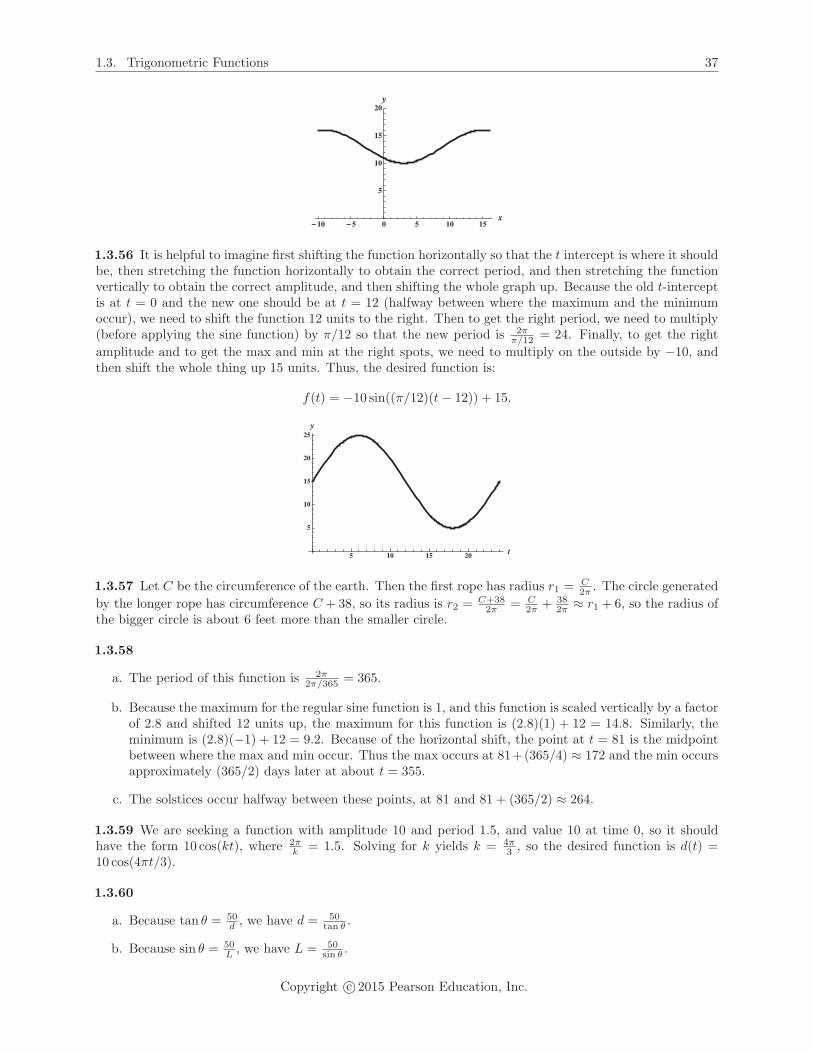
f(t) = −10 sin((π/12)(t− 12)) + 15.
5 10 15 20 t
5
10
15
20
25y
1.3.57 Let C be the circumference of the earth. Then the first rope has radius r1 = C2π . The circle generated
by the longer rope has circumference C + 38, so its radius is r2 = C+382π = C
2π + 382π ≈ r1 + 6, so the radius of
the bigger circle is about 6 feet more than the smaller circle.
1.3.58
a. The period of this function is 2π2π/365 = 365.
b. Because the maximum for the regular sine function is 1, and this function is scaled vertically by a factorof 2.8 and shifted 12 units up, the maximum for this function is (2.8)(1) + 12 = 14.8. Similarly, theminimum is (2.8)(−1) + 12 = 9.2. Because of the horizontal shift, the point at t = 81 is the midpointbetween where the max and min occur. Thus the max occurs at 81+(365/4) ≈ 172 and the min occursapproximately (365/2) days later at about t = 355.
c. The solstices occur halfway between these points, at 81 and 81 + (365/2) ≈ 264.
1.3.59 We are seeking a function with amplitude 10 and period 1.5, and value 10 at time 0, so it shouldhave the form 10 cos(kt), where 2π
k = 1.5. Solving for k yields k = 4π3 , so the desired function is d(t) =
10 cos(4πt/3).
1.3.60
a. Because tan θ = 50d , we have d = 50
tan θ .
b. Because sin θ = 50L , we have L = 50
sin θ .
Copyright c© 2015 Pearson Education, Inc.

38 Chapter 1. Functions
1.3.61 Let L be the line segment connecting the tops of the ladders and let M be the horizontal linesegment between the walls h feet above the ground. Now note that the triangle formed by the ladders and Lis equilateral, because the angle between the ladders is 60 degrees, and the other two angles must be equaland add to 120, so they are 60 degrees as well. Now we can see that the triangle formed by L, M and theright wall is similar to the triangle formed by the left ladder, the left wall, and the ground, because they areboth right triangles with one angle of 75 degrees and one of 15 degrees. Thus M = h is the distance betweenthe walls.
1.3.62 Let the corner point P divide the pole into two pieces, L1 (which spans the 3-ft hallway) and L2
(which spans the 4-ft hallway.) Then L = L1 + L2. Now L2 = 4sin θ , and
3L1
= cos θ (see diagram.) Thus
L = L1 + L2 = 3cos θ + 4
sin θ . When L = 10, θ ≈ .9273.
Θ P3
4
L1
L2
Θ
1.3.63 To find s(t) note that we are seeking a periodic function with period 365, and with amplitude 87.5(which is half of the number of minutes between 7:25 and 4:30). We need to shift the function 4 days plusone fourth of 365, which is about 95 days so that the max and min occur at t = 4 days and at half a yearlater. Also, to get the right value for the maximum and minimum, we need to multiply by negative one andadd 117.5 (which represents 30 minutes plus half the amplitude, because s = 0 corresponds to 4:00 AM.)Thus we have
s(t) = 117.5− 87.5 sin( π
182.5(t− 95)
).
A similar analysis leads to the formula
S(t) = 844.5 + 87.5 sin( π
182.5(t− 67)
).
The graph pictured shows D(t) = S(t)− s(t), the length of day function, which has its max at the summersolstice which is about the 172nd day of the year, and its min at the winter solstice.
�50 50 100 150 200 250 300t
200
400
600
800
D
1.3.64 Let θ1 be the viewing angle to the bottom of the television. Then tan θ1 =(
310
). Now tan(θ+ θ1) =
1010 = 1, so θ + θ1 = π
4 , so θ = π4 − θ1 ≈ 0.494.
1.3.65 The area of the entire circle is πr2. The ratio θ2π represents the proportion of the area swept out
by a central angle θ. Thus the area of a sector of a circle is this same proportion of the entire area, so it isθ2π · πr2 = r2θ
2 .
Copyright c© 2015 Pearson Education, Inc.

Chapter One Review 39
1.3.66 Using the given diagram, drop a perpendicular from the point (b cos θ, b sin θ) to the x axis, andconsider the right triangle thus formed whose hypotenuse has length c. By the Pythagorean theorem,(b sin θ)2 + (a− b cos θ)2 = c2. Expanding the binomial gives b2 sin2 θ + a2 − 2ab cos θ + b2 cos2 θ = c2. Nowbecause b2 sin2 θ + b2 cos2 θ = b2, this reduces to a2 + b2 − 2ab cos θ = c2.
1.3.67 Note that sinA = hc and sinC = h
a , so h = c sinA = a sinC. Thus
sinA
a=
sinC
c.
Now drop a perpendicular from the vertex A to the line determined by BC, and let h2 be the length ofthis perpendicular. Then sinC = h2
b and sinB = h2
C , so h2 = b sinC = c sinB. Thus
sinC
c=
sinB
b.
Putting the two displayed equations together gives
sinA
a=
sinB
b=
sinC
c.
Chapter One Review
1
a. True. For example, f(x) = x2 is such a function.
b. False. For example, cos(π/2 + π/2) = cos(π) = −1 = cos(π/2) + cos(π/2) = 0 + 0 = 0.
c. False. Consider f(1 + 1) = f(2) = 2m + b = f(1) + f(1) = (m + b) + (m + b) = 2m + 2b. (At leastthese aren’t equal when b = 0.)
d. True. f(f(x)) = f(1− x) = 1− (1− x) = x.
e. False. This set is the union of the disjoint intervals (−∞,−7) and (1,∞).
2
a. Because the quantity under the radical must be non-zero, the domain of f is [0,∞). The range is also[0,∞).
b. The domain is (−∞, 2)∪ (2,∞). The range is (−∞, 0)∪ (0,∞). (Note that if 0 were in the range then1
y−2 = 0 for some value of y, but this expression has no real solutions.)
c. Because h can be written h(z) =√(z − 3)(z + 1), we see that the domain is (−∞,−1] ∪ [3,∞). The
range is [0,∞). (Note that as z gets large, h(z) gets large as well.)
Copyright c© 2015 Pearson Education, Inc.

40 Chapter 1. Functions
3
a.
This line has slope 2−(−3)4−2 = 5/2. Therefore the
equation of the line is y − 2 = 52 (x − 4), so y =
52x− 8.
�2 �1 1 2 3 4x
�12
�10
�8
�6
�4
�2
2y
b.
This line has the form y = (3/4)x+b, and because(−4, 0) is on the line, 0 = (3/4)(−4) + b, so b =3. Thus the equation of the line is given by y =(3/4)x+ 3.
�6 �4 �2 2 4x
�2
2
4
6y
c.This line has slope 0−(−2)
4−0 = 12 , and the y-intercept
is given to be −2, so the equation of this line isy = (1/2)x− 2.
�4 �2 2 4 6x
�4
�3
�2
�1
1y
4
The function is a piecewise step function whichjumps up by one every half-hour step.
0.5 1.0 1.5 2.0 2.5 3.0x
1
2
3
4
5
6
7
y
Copyright c© 2015 Pearson Education, Inc.

Chapter One Review 41
5
Because |x| =⎧⎨⎩−x if x < 0;
x if x ≥ 0,we have
2(x− |x|) =⎧⎨⎩2(x− (−x)) = 4x if x < 0;
2(x− x) = 0 if x ≥ 0.
�2 �1 1 2x
�8
�6
�4
�2
y
6 Because the trip is 500 miles in a car that gets 35 miles per gallon, 50035 = 100
7 represents the number ofgallons required for the trip. If we multiply this times the number of dollars per gallon we will get the cost.Thus C = f(p) = 100
7 p dollars.
7
a.This is a straight line with slope 2/3 and y-intercept 10/3.
�2 �1 0 1 2x
1
2
3
4
5y
b.Completing the square gives y = (x2+2x+1)−4,or y = (x+1)2−4, so this is the standard parabolashifted one unit to the left and down 4 units. �4 �3 �2 �1 1 2
x
�4
�2
2
4
y
c.Completing the square, we have x2+2x+1+y2+4y+4 = −1+1+4, so we have (x+1)2+(y+2)2 = 4,a circle of radius 2 centered at (−1,−2).
�3 �2 �1 1x
�4
�3
�2
�1
y
Copyright c© 2015 Pearson Education, Inc.

42 Chapter 1. Functions
d.Completing the square, we have x2−2x+1+y2−8y+16 = −5+1+16, or (x− 1)2+(y− 4)2 = 12,which is a circle of radius
√12 centered at (1, 4).
�2 �1 0 1 2 3 4x
2
4
6
8y
8
To solve x1/3 = x1/4 we raise each side to the 12thpower, yielding x4 = x3. This gives x4−x3 = 0, orx3(x− 1) = 0, so the only solutions are x = 0 andx = 1 (which can be easily verified as solutions.)Between 0 and 1, x1/4 > x1/3, but for x > 1,x1/3 > x1/4.
1 2 3 4x
0.5
1.0
1.5
y
9 The domain of x1/7 is the set of all real numbers, as is its range. The domain of x1/4 is the set ofnon-negative real numbers, as is its range.
10
Completing the square in the second equation, wehave x2 + y2 − 7y + 49
4 = −8 + 494 , which can be
written as x2+(y− (7/2))2 = 174 . Thus we have a
circle of radius√17/2 centered at (0, 7/2), along
with the standard parabola. These intersect wheny = 7y−y2−8, which occurs for y2−6y+8 = 0, sofor y = 2 and y = 4, with corresponding x valuesof ±2 and ±√
2.
�3 �2 �1 1 2 3x
2
4
6
8
y
11 We are looking for the line between the points (0, 212) and (6000, 200). The slope is 212−2000−6000 = − 12
6000 =
− 1500 . Because the intercept is given, we deduce that the line is B = f(a) = − 1
500a+ 212.
12
a. The cost of producing x books is C(x) = 1000 + 2.5x.
b. The revenue generated by selling x books is R(x) = 7x.
Copyright c© 2015 Pearson Education, Inc.

Chapter One Review 43
c.The break-even point is where R(x) = C(x). Thisis where 7x = 1000 + 2.5x, or 4.5x = 1000. Sox = 1000
4.5 ≈ 222.
100 200 300 400x
500
1000
1500
2000
2500
y
13
a.
y�x2
y��x�3�2
�10 �5 5 x
20
40
60
80
100
y
b.
y�2�x�4�2
y�x2
�10 �5 5 10 15 x
100
200
300
400y
c.
y�x2
y���3x�2
�10 �5 5 10 x
�800
�600
�400
�200
y
d.
y�x2
y��2�x�3��2
�4 �2 0 2 4 6 8 x
10
20
30
40
50
60y
Copyright c© 2015 Pearson Education, Inc.

44 Chapter 1. Functions
14
a.
�4 �2 2 4x
�5
5
y
b.
�4 �2 2 4x
�10
�5
5
10
y
c.
�6 �4 �2 2 4 6x
�5
5
y
d.
�4 �2 2 4x
�5
5
y
15
a. h(g(π/2)) = h(1) = 1
b. h(f(x)) = h(x3) = x3/2.
c. f(g(h(x))) = f(g(√x)) = f(sin(
√x)) = (sin(
√x))3.
d The domain of g(f(x)) is R, because the domain of both functions is the set of all real numbers.
e. The range of f(g(x)) is [−1, 1]. This is because the range of g is [−1, 1], and on the restricted domain[−1, 1], the range of f is also [−1, 1].
16
a. If g(x) = x2 + 1 and f(x) = sinx, then f(g(x)) = f(x2 + 1) = sin(x2 + 1).
b. If g(x) = x2 − 4 and f(x) = x−3 then f(g(x)) = f(x2 − 4) = (x2 − 4)−3.
17 f(x+h)−f(x)h = (x+h)2−2(x+h)−(x2−2x)
h = x2+2hx+h2−2x−2h−x2+2xh = 2hx+h2−2h
h = 2x+ h− 2.
f(x)−f(a)x−a = x2−2x−(a2−2a)
x−a = (x2−a2)−2(x−a)x−a = (x−a)(x+a)−2(x−a)
x−a = x+ a− 2.
18 f(x+h)−f(x)h = 4−5(x+h)−(4−5x)
h = 4−5x−5h−4+5xh = − 5h
h = −5.
f(x)−f(a)x−a = 4−5x−(4−5a)
x−a = − 5(x−a)x−a = −5.
19 f(x+h)−f(x)h = (x+h)3+2−(x3+2)
h = x3+3x2h+3xh2+h3+2−x3−2h = h(3x2+3xh+h2)
h = 3x2 + 3xh+ h2.
f(x)−f(a)x−a = x3+2−(a3+2)
x−a = x3−a3
x−a = (x−a)(x2+ax+a2)x−a = x2 + ax+ a2.
20 f(x+h)−f(x)h =
7x+h+3− 7
x+3
h =7x+21−(7x+7h+21)
(x+3)(x+h+3)
h = − 7h(h)(x+3)(x+h+3) = − 7
(x+3)(x+h+3) .
f(x)−f(a)x−a =
7x+3− 7
a+3
x−a =7a+21−(7x+21)
(x+3)(a+3)
x−a = − 7(x−a)(x−a)(x+3)(a+3) = − 7
(x+3)(a+3) .
Copyright c© 2015 Pearson Education, Inc.

Chapter One Review 45
21
a. Because f(−x) = cos−3x = cos 3x = f(x), this is an even function, and is symmetric about the y-axis.
b. Because f(−x) = 3(−x)4 − 3(−x)2 + 1 = 3x4 − 3x2 + 1 = f(x), this is an even function, and issymmetric about the y-axis.
c. Because replacing x by −x and/or replacing y by −y gives the same equation, this represents a curvewhich is symmetric about the y-axis and about the origin and about the x-axis.
22
a. 1+cos θsin θ = 1+cos θ
sin θ · 1−cos θ1−cos θ = 1−cos2 θ
(sin θ)(1−cos θ) =sin2 θ
(sin θ)(1−cos θ) =sin θ
1−cos θ .
b. sec θ−1tan θ = sec θ−1
tan θ · sec θ+1sec θ+1 = sec2 θ−1
(tan θ)(sec θ+1) =tan2 θ
(tan θ)(sec θ+1) =tan θ
sec θ+1 .
23
a. A 135 degree angle measures 135 · (π/180) radians, which is 3π/4 radians.
b. A 4π/5 radian angle measues 4π/5 · (180/π) degrees, which is 144 degrees.
c. Because the length of the arc is the measure of the subtended angle (in radians) times the radius, thisarc would be 4π/3 · 10 = 40π
3 units long.
24
a. This function has period 2π1/2 = 4π and amplitude
4. �10 �5 5 10x
�4
�2
2
4y
b. This function has period 2π2π/3 = 3 and amplitude
2. �3 �2 �1 1 2 3Θ
�2
�1
1
2y
c.
This function has period 2π2 = π and amplitude
1. Compared to the ordinary cosine function it iscompressed horizontally, flipped about the x-axis,and shifted π/4 units to the right.
�3 �2 �1 1 2 3Θ
�1.0
�0.5
0.5
1.0y
Copyright c© 2015 Pearson Education, Inc.

46 Chapter 1. Functions
25
a. We need to scale the ordinary cosine function so that its period is 6, and then shift it 3 units to theright, and multiply it by 2. So the function we seek is y = 2 cos((π/3)(t− 3)) = −2 cos(πt/3).
b. We need to scale the ordinary cosine function so that its period is 24, and then shift it to the right6 units. We then need to change the amplitude to be half the difference between the maximum andminimum, which would be 5. Then finally we need to shift the whole thing up by 15 units. Thefunction we seek is thus y = 15 + 5 cos((π/12)(t− 6)) = 15 + 5 sin(πt/12).
26 The pictured function has a period of π, an amplitude of 2, and a maximum of 3 and a minimum of −1.It can be described by y = 1 + 2 cos(2(x− π/2)).
27
a. − sinx is pictured in F.
b. cos 2x is pictured in E.
c. tan(x/2) is pictured in D.
d. − secx is pictured in B.
e. cot 2x is pictured in C.
f. sin2 x is pictured in A.
28 If secx = 2, then cosx = 12 . This occurs for x = −π/3 and x = π/3, so the intersection points are
(−π/3, 2) and (π/3, 2).
29 sinx = − 12 for x = 7π/6 and for x = 11π/6, so the intersection points are (7π/6,−1/2) and (11π/6,−1/2).
30 Let N be the north pole, and C the center of the given circle, and consider the angle CNP . This anglemeasures π−ϕ
2 . (Note that the triangle CNP is isosceles.) Now consider the triangle NOX where O is the
origin and X is the point (x, 0). Using triangle NOX, we have tan(π−ϕ2
)= x
2R , so x = 2R tan(π−ϕ2
).
Copyright c© 2015 Pearson Education, Inc.

Chapter 2
Limits
2.1 The Idea of Limits
2.1.1 The average velocity of the object between time t = a and t = b is the change in position divided by
the elapsed time: vav = s(b)−s(a)b−a .
2.1.2 In order to compute the instantaneous velocity of the object at time t = a, we compute the average
velocity over smaller and smaller time intervals of the form [a, t], using the formula: vav = s(t)−s(a)t−a . We let t
approach a. If the quantity s(t)−s(a)t−a approaches a limit as t → a, then that limit is called the instantaneous
velocity of the object at time t = a.
2.1.3 The slope of the secant line between points (a, f(a)) and (b, f(b)) is the ratio of the differences f(b)−f(a) and b− a. Thus msec =
f(b)−f(a)b−a .
2.1.4 In order to compute the slope of the tangent line to the graph of y = f(t) at (a, f(a)), we compute the
slope of the secant line over smaller and smaller time intervals of the form [a, t]. Thus we consider f(t)−f(a)t−a
and let t → a. If this quantity approaches a limit, then that limit is the slope of the tangent line to the curvey = f(t) at t = a.
2.1.5 Both problems involve the same mathematics, namely finding the limit as t → a of a quotient of
differences of the form g(t)−g(a)t−a for some function g.
2.1.6
Because f(x) = x2 is an even function, f(−a) =f(a) for all a. Thus the slope of the secant linebetween the points (a, f(a)) and (−a, f(−a)) is
msec = f(−a)−f(a)−a−a = 0
−2a = 0. The slope of thetangent line at x = 0 is also zero.
�a, f �a����a, f ��a��
�4 �2 2 4 x
5
10
15
20
y
2.1.7 The average velocity is s(3)−s(2)3−2 = 156− 136 = 20.
2.1.8 The average velocity is s(4)−s(1)4−1 = 144−84
3 = 603 = 20.
47

48 Chapter 2. Limits
2.1.9
a. Over [1, 4], we have vav = s(4)−s(1)4−1 = 256−112
3 = 48.
b. Over [1, 3], we have vav = s(3)−s(1)3−1 = 240−112
2 = 64.
c. Over [1, 2], we have vav = s(2)−s(1)2−1 = 192−112
1 = 80.
d. Over [1, 1+h], we have vav = s(1+h)−s(1)1+h−1 = −16(1+h)2+128(1+h)−(112)
h = −16h2−32h+128hh = h(−16h+96)
h =96− 16h = 16(6− h).
2.1.10
a. Over [0, 3], we have vav = s(3)−s(0)3−0 = 65.9−20
3 = 15.3.
b. Over [0, 2], we have vav = s(2)−s(0)2−0 = 60.4−20
2 = 20.2.
c. Over [0, 1], we have vav = s(1)−s(0)1−0 = 45.1−20
1 = 25.1.
d. Over [0, h], we have vav = s(h)−s(0)h−0 = −4.9h2+30h+20−20
h = (h)(−4.9h+30)h = −4.9h+ 30.
2.1.11
a. s(2)−s(0)2−0 = 72−0
2 = 36.
b. s(1.5)−s(0)1.5−0 = 66−0
1.5 = 44.
c. s(1)−s(0)1−0 = 52−0
1 = 52.
d. s(0.5)−s(0)0.5−0 = 30−0
0.5 = 60.
2.1.12
a. s(2.5)−s(0.5)2.5−0.5 = 150−46
2 = 52.
b. s(2)−s(0.5)2−0.5 = 136−46
1.5 = 60.
c. s(1.5)−s(0.5)1.5−0.5 = 114−46
1 = 68.
d. s(1)−s(0.5)1−0.5 = 84−46
0.5 = 76.
2.1.13
0.5 1.0 1.5 2.0 2.5 t
50
100
150
s
The slope of the secant line is given bys(2)−s(0.5)
2−0.5 = 136−461.5 = 60. This represents the av-
erage velocity of the object over the time interval[0.5, 2].
Copyright c© 2015 Pearson Education, Inc.

2.1. The Idea of Limits 49
2.1.14
0.1 0.2 0.3 0.4 0.5 0.6 t
0.2
0.4
0.6
0.8
1.0
1.2s
The slope of the secant line is given bys(0.5)−s(0)
0.5−0 = 10.5 = 2. This represents the aver-
age velocity of the object over the time interval[0, 0.5].
2.1.15Time Interval [1, 2] [1, 1.5] [1, 1.1] [1, 1.01] [1, 1.001]
Average Velocity 80 88 94.4 95.84 95.984
The instantaneous velocity appears to be 96 ft/s.
2.1.16Time Interval [2, 3] [2, 2.25] [2, 2.1] [2, 2.01] [2, 2.001]
Average Velocity 5.5 9.175 9.91 10.351 10.395
The instantaneous velocity appears to be 10.4 m/s.
2.1.17 s(1.01)−s(1)0.01 = 47.84, while s(1.001)−s(1)
0.001 = 47.984 and s(1.0001)−s(1)0.0001 = 47.9984. It appears that the
instantaneous velocity at t = 1 is approximately 48.
2.1.18 s(2.01)−s(2)0.01 = −4.16, while s(2.001)−s(2)
0.001 = −4.016 and s(2.0001)−s(2)0.0001 = −4.0016. It appears that the
instantaneous velocity at t = 2 is approximately −4.
2.1.19Time Interval [2, 3] [2.9, 3] [2.99, 3] [2.999, 3] [2.9999, 3] [2.99999, 3]
Average Velocity 20 5.6 4.16 4.016 4.002 4.0002
The instantaneous velocity appears to be 4 ft/s.
2.1.20Time Interval [π/2, π] [π/2, π/2 + 0.1] [π/2, π/2 + .01] [π/2, π/2 + .001] [π/2, π/2 + .0001]
Average Velocity −1.90986 −0.149875 −0.0149999 −0.0015 −0.00015
The instantaneous velocity appears to be 0 ft/s.
2.1.21Time Interval [3, 3.1] [3, 3.01] [3, 3.001] [3, 3.0001]
Average Velocity −17.6 −16.16 −16.016 −16.002
The instantaneous velocity appears to be −16 ft/s.
2.1.22Time Interval [π/2, π/2 + 0.1] [π/2, π/2 + 0.01] [π/2, π/2 + 0.001] [π/2, π/2 + 0.0001]
Average Velocity −19.9667 −19.9997 −20.0000 −20.0000
The instantaneous velocity appears to be −20 ft/s.
2.1.23Time Interval [0, 0.1] [0, 0.01] [0, 0.001] [0, 0.0001]
Average Velocity 79.468 79.995 80.000 80.0000
The instantaneous velocity appears to be 80 ft/s.
2.1.24Time Interval [0, 1] [0, 0.1] [0, 0.01] [0, 0.001]
Average Velocity −10 −18.1818 −19.802 −19.98
The instantaneous velocity appears to be −20 ft/s.
Copyright c© 2015 Pearson Education, Inc.

50 Chapter 2. Limits
2.1.25x Interval [2, 2.1] [2, 2.01] [2, 2.001] [2, 2.0001]
Slope of Secant Line 8.2 8.02 8.002 8.0002
The slope of the tangent line appears to be 8.
2.1.26x Interval [π/2, π/2 + 0.1] [π/2, π/2 + 0.01] [π/2, π/2 + 0.001] [π/2, π/2 + 0.0001]
Slope of Secant Line −2.995 −2.99995 −3.0000 −3.0000
The slope of the tangent line appears to be −3.
2.1.27x Interval [−1,−0.9] [−1,−0.99] [−1,−0.999] [−1,−0.9999]
Slope of the Secant Line 0.524862 0.5025 0.50025 0.500025
The slope of the tangent line appears to be 0.5.
2.1.28x Interval [1, 1.1] [1, 1.01] [1, 1.001] [1, 1.0001]
Slope of the Secant Line 2.31 2.0301 2.003 2.0003
The slope of the tangent line appears to be 2.
2.1.29
a. Note that the graph is a parabola with ver-tex (2,−1).
b. At (2,−1) the function has tangent line withslope 0.
�1 1 2 3 4 5x
2
4
6
8y
c.x Interval [2, 2.1] [2, 2.01] [2, 2.001] [2, 2.0001]
Slope of the Secant Line .1 .01 .001 .0001
The slope of the tangent line at (2,−1) appears to be 0.
2.1.30
a. Note that the graph is a parabola with ver-tex (0, 4).
b. At (0, 4) the function has a tangent line withslope 0.
c. This is true for this function – because thefunction is symmetric about the y-axis andwe are taking pairs of points symmetricallyabout the y axis. Thus f(0 + h) = 4− (0 +h)2 = 4− (−h)2 = f(0− h). So the slope of
any such secant line is 4−h2−(4−h2)h−(−h) = 0
2h =0.
�2 �1 1 2x
�2
�1
1
2
3
4y
Copyright c© 2015 Pearson Education, Inc.

2.1. The Idea of Limits 51
2.1.31
a. Note that the graph is a parabola with ver-tex (4, 448).
b. At (4, 448) the function has tangent line withslope 0, so a = 4.
2 4 6 8x
100
200
300
400
y
c.x Interval [4, 4.1] [4, 4.01] [4, 4.001] [4, 4.0001]
Slope of the Secant Line −1.6 −0.16 −0.016 −0.0016
The slopes of the secant lines appear to beapproaching zero.
d. On the interval [0, 4) the instantaneous ve-locity of the projectile is positive.
e. On the interval (4, 9] the instantaneous ve-locity of the projectile is negative.
2.1.32
a. The rock strikes the water when s(t) = 96. This occurs when 16t2 = 96, or t2 = 6, whose only positivesolution is t =
√6 ≈ 2.45 seconds.
b.t Interval [
√6− 0.1,
√6] [
√6− 0.01,
√6] [
√6− 0.001,
√6] [
√6− 0.0001,
√6]
Average Velocity 76.7837 78.2237 78.3677 78.3821
When the rock strikes the water, its instantaneous velocity is about 78.38 ft/s.
2.1.33 For line AD, we have
mAD =yD − yAxD − xA
=f(π)− f(π/2)
π − (π/2)=
1
π/2≈ .63662.
For line AC, we have
mAC =yC − yAxC − xA
=f(π/2 + 0.5)− f(π/2)
(π/2 + 0.5)− (π/2)= −cos(π/2 + 0.5)
0.5≈ 0.958851.
For line AB, we have
mAB =yB − yAxB − xA
=f(π/2 + 0.05)− f(π/2)
(π/2 + 0.05)− (π/2)= −cos(π/2 + 0.05)
0.05≈ 0.999583.
Computing one more slope of a secant line:
msec =f(π/2 + 0.01)− f(π/2)
(π/2 + 0.01)− (π/2)= −cos(π/2 + 0.01)
0.01≈ 0.999983.
Conjecture: The slope of the tangent line to the graph of f at x = π/2 is 1.
Copyright c© 2015 Pearson Education, Inc.
52 Chapter 2. Limits
2.2 Definitions of Limits
2.2.1 Suppose the function f is defined for all x near a except possibly at a. If f(x) is arbitrarily close to anumber L whenever x is sufficiently close to (but not equal to) a, then we write lim
x→af(x) = L.
2.2.2 False. For example, consider the function f(x) =
⎧⎨⎩x2 if x = 0
4 if x = 0.
Then limx→0
f(x) = 0, but f(0) = 4.
2.2.3 Suppose the function f is defined for all x near a but greater than a. If f(x) is arbitrarily close to Lfor x sufficiently close to (but strictly greater than) a, then we write lim
x→a+f(x) = L.
2.2.4 Suppose the function f is defined for all x near a but less than a. If f(x) is arbitrarily close to L forx sufficiently close to (but strictly less than) a, then we write lim
x→a−f(x) = L.
2.2.5 It must be true that L = M .
2.2.6 Because graphing utilities generally just plot a sampling of points and “connect the dots,” they cansometimes mislead the user investigating the subtleties of limits.
2.2.7
a. h(2) = 5.
b. limx→2
h(x) = 3.
c. h(4) does not exist.
d. limx→4
f(x) = 1.
e. limx→5
h(x) = 2.
2.2.8
a. g(0) = 0.
b. limx→0
g(x) = 1.
c. g(1) = 2.
d. limx→1
g(x) = 2.
2.2.9
a. f(1) = −1.
b. limx→1
f(x) = 1.
c. f(0) = 2.
d. limx→0
f(x) = 2.
2.2.10
a. f(2) = 2.
b. limx→2
f(x) = 4.
c. limx→4
f(x) = 4.
d. limx→5
f(x) = 2.
2.2.11
a.x 1.9 1.99 1.999 1.9999 2 2.0001 2.001 2.01 2.1
f(x) = x2−4x−2 3.9 3.99 3.999 3.9999 undefined 4.0001 4.001 4.01 4.1
b. limx→2
f(x) = 4.
2.2.12
a.x .9 .99 .999 .9999 1 1.0001 1.001 1.01 1.1
f(x) = x3−1x−1 2.71 2.9701 2.997 2.9997 undefined 3.0003 3.003 3.0301 3.31
b. limx→1
x3 − 1
x− 1= 3
Copyright c© 2015 Pearson Education, Inc.

2.2. Definitions of Limits 53
2.2.13
a.t 8.9 8.99 8.999 9 9.001 9.01 9.1
g(t) = t−9√t−3
5.98329 5.99833 5.99983 undefined 6.00017 6.00167 6.01662
b. limt→9
t− 9√t− 3
= 6.
2.2.14
a.x .01 .001 .0001 .00001
f(x) = (1 + x)1/x 2.70481 2.71692 2.71815 2.71827
x −0.01 −0.001 −0.0001 −0.00001
f(x) = (1 + x)1/x 2.732 2.71964 2.71842 2.71830
b. limx→0
(1 + x)1/x ≈ 2.718.
c. limx→0
(1 + x)1/x = e.
2.2.15
a.
0 1 2 3 4 x
0.5
1.0
1.5
2.0y
b.x 1.8 1.9 1.99 2.01 2.1 2.2
f(x) 1.0067 1.00167 1.00002 1.00002 1.00167 1.0067
From both the graph and the table, the limit appears to be 1.
2.2.16
a.
�1.0 �0.5 0.5 1.0 x
0.5
1.0
1.5
2.0
2.5
y
b.x −0.2 −0.1 −0.01 0.01 0.1 0.2
f(x) 2.03336 2.00834 2.00008 2.00008 2.00834 2.03336
From both the graph and the table, the limit appears to be 2.
Copyright c© 2015 Pearson Education, Inc.

54 Chapter 2. Limits
2.2.17
a.
�1 1 2 3 x
0.5
1.0
1.5
2.0y
b.x 0.9 0.99 0.999 1.001 1.01 1.1
f(x) 1.993342 1.999933 1.999999 1.999999 1.999933 1.993342
From both the graph and the table, the limit appears to be 2.
2.2.18
a.
�1 1 2 3 x
0.5
1.0
1.5
2.0
2.5
3.0
3.5y
b.x −0.1 −0.01 −0.001 0.001 0.01 0.1
f(x) 2.8951 2.99 2.999 3.001 3.0099 3.0949
From both the graph and the table, the limit appears to be 3.
2.2.19
x 4.9 4.99 4.999 4.9999 5 5.0001 5.001 5.01 5.1
f(x) = x2−25x−5 9.9 9.99 9.999 9.9999 undefined 10.0001 10.001 10.01 10.1
limx→5+
x2 − 25
x− 5= 10, lim
x→5−
x2 − 25
x− 5= 10, and thus lim
x→5
x2 − 25
x− 5= 10.
2.2.20
x 99.9 99.99 99.999 99.9999 100 100.0001 100.001 100.01 100.1
f(x) = x−100√x−10
19.995 19.9995 19.99995 ≈ 20 undefined ≈ 20 20.0005 20.00005 20.005
limx→100+
x− 100√x− 10
= 20, limx→100−
x− 100√x− 10
= 20, and thus limx→100
x− 100√x− 10
= 20.
2.2.21
a. f(1) = 0. b. limx→1−
f(x) = 1. c. limx→1+
f(x) = 0.
d. limx→1
f(x) does not exist, since the two one-sided limits aren’t equal.
Copyright c© 2015 Pearson Education, Inc.

2.2. Definitions of Limits 55
2.2.22
a. g(2) = 3. b. limx→2−
g(x) = 2. c. limx→2+
g(x) = 3.
d. limx→2
g(x) does not exist. e. g(3) = 2. f. limx→3−
g(x) = 3.
g. limx→3+
g(x) = 2. h. g(4) = 3. i. limx→4
g(x) = 3.
2.2.23
a. f(1) = 3. b. limx→1−
f(x) = 2. c. limx→1+
f(x) = 2.
d. limx→1
f(x) = 2. e. f(3) = 2. f. limx→3−
f(x) = 4.
g. limx→3+
f(x) = 1. h. limx→3
f(x) does not exist. i. f(2) = 3.
j. limx→2−
f(x) = 3. k. limx→2+
f(x) = 3. l. limx→2
f(x) = 3.
2.2.24
a. g(−1) = 3. b. limx→−1−
g(x) = 2. c. limx→−1+
g(x) = 2.
d. limx→−1
g(x) = 2. e. g(1) = 2. f. limx→1
g(x) does not exist.
g. limx→3
g(x) = 4. h. g(5) = 5. i. limx→5−
g(x) = 5.
2.2.25
a.x 2
π23π
25π
27π
29π
211π
f(x) = sin(1/x) 1 −1 1 −1 1 −1
If xn = 2(2n+1)π , then f(xn) = (−1)n where n is a non-negative integer.
b. As x → 0, 1/x → ∞. So the values of f(x) oscillate dramatically between −1 and 1.
c. limx→0
sin(1/x) does not exist.
2.2.26
a.x 12
π123π
125π
127π
129π
1211π
f(x) = tan(3/x) 1 −1 1 −1 1 −1
We have alternating 1’s and −1’s.
b.tan 3x alternates between 1 and −1 infinitelymany times on (0, h) for any h > 0.
�0.5 0.5 1.0 1.5 2.0 2.5x
�10
�5
5
10
y
c. limx→0
tan(3/x) does not exist.
2.2.27
a. False. In fact limx→3
x2 − 9
x− 3= lim
x→3(x+ 3) = 6.
Copyright c© 2015 Pearson Education, Inc.

56 Chapter 2. Limits
b. False. For example, if f(x) =
⎧⎨⎩x2 if x = 0;
5 if x = 0and if a = 0 then f(a) = 5 but lim
x→af(x) = 0.
c. False. For example, the limit in part a of this problem exists, even though the corresponding functionis undefined at a = 3.
d. False. It is true that the limit of√x as x approaches zero from the right is zero, but because the
domain of√x does not include any numbers to the left of zero, the two-sided limit doesn’t exist.
e. True. Note that limx→π/2
cosx = 0 and limx→π/2
sinx = 1, so limx→π/2
cosx
sinx=
0
1= 0.
2.2.28
0.5 1.0 1.5 2.0 2.5 3.0 t
�4
�2
2
4
6y
2.2.29
1 2 3 4 x
�3
�2
�1
1
y
2.2.30
�2 �1 1 2 x
1
2
3
4y
2.2.31
�2 �1 1 2 3 4 x
0.5
1.0
1.5
2.0
2.5
3.0y
2.2.32
h 0.01 0.001 0.0001 −0.01 −0.001 −0.0001
sin(h)/h 0.99998 0.9999998 0.999999998 0.99998 0.9999998 0.999999998
limh→0
sin(h)
h= 1
2.2.33
h 0.01 0.001 0.0001 −0.01 −0.001 −0.0001
tan(3h)/h 3.0009 3.000009 3.00000009 3.0009 3.000009 3.00000009
limh→0
tan(3h)
h= 3
2.2.34
h 0.01 0.001 0.0001 −0.01 −0.001 −0.0001
(√(h+ 4)− 2)/h 0.24984 0.249984 0.25000 0.250156 0.250016 0.25000
Copyright c© 2015 Pearson Education, Inc.

2.2. Definitions of Limits 57
limh→0
√h+ 4− 2
h=
1
4
2.2.35
h 0.01 0.001 0.0001 −0.01 −0.001 −0.0001
(1− cos(h))/h 0.0049999 0.0005 0.00005 −0.0049999 −0.0005 −0.00005
limh→0
1− cos(h)
h= 0
2.2.36
a. Note that f(x) = |x|x is undefined at 0, and
limx→0−
f(x) = −1 and limx→0+
f(x) = 1.
b. limx→0
f(x) does not exist, since the two one-
side limits aren’t equal.
�2 �1 1 2 m
�1.0
�0.5
0.5
1.0
y
2.2.37
a. limx→−1−
�x = −2, limx→−1+
�x = −1, limx→2−
�x = 1, limx→2+
�x = 2.
b. limx→2.3−
�x = 2, limx→2.3+
�x = 2, limx→2.3
�x = 2.
c. In general, for an integer a, limx→a−
�x = a− 1 and limx→a+
�x = a.
d. In general, if a is not an integer, limx→a−
�x = limx→a+
�x = �a .
e. limx→a
�x exists and is equal to �a for non-integers a.
2.2.38
a. Note that the graph is piecewise constant.
b. limx→2−
�x� = 2, limx→1+
�x� = 2, limx→1.5
�x� = 2.
c. limx→a
�x� exists and is equal to �a� for non-
integers a. �2 �1 1 2 3x
�1
1
2
3y
2.2.39 By zooming in closely, you should be able to convince yourself that the answer is 0.
2.2.40 By zooming in closely, you should be able to convince yourself that the answer is 2.
2.2.41 By zooming in closely, you should be able to convince yourself that the answer is 16.
2.2.42 By zooming in closely, you should be able to convince yourself that the answer is 0.
Copyright c© 2015 Pearson Education, Inc.

58 Chapter 2. Limits
2.2.43
a. Note that the function is piecewise constant.
b. limw→3.3
f(w) = .95.
c. limw→1+
f(w) = .61 corresponds to the fact
that for any piece of mail that weighs slightlyover 1 ounce, the postage will cost 61 cents.lim
w→1−f(w) = .44 corresponds to the fact
that for any piece of mail that weighs slightlyless than 1 ounce, the postage will cost 44cents.
d. limw→4
f(w) does not exist because the two cor-
responding one-side limits don’t exist. (Thelimit from the left is .95, while the limit fromthe right is 1.12.)
1 2 3 4 5x
0.2
0.4
0.6
0.8
1.0
y
2.2.44
a. Note that H is piecewise constant.
b. limx→0−
H(x) = 0, limx→0+
H(x) = 1, and so
limx→0
H(x) does not exist.
�1.0 �0.5 0.5 1.0x
0.2
0.4
0.6
0.8
1.0
1.2
y
2.2.45
a. Because of the symmetry about the y axis, we must have limx→−2+
f(x) = 8.
b. Because of the symmetry about the y axis, we must have limx→−2−
f(x) = 5.
2.2.46
a. Because of the symmetry about the origin, we must have limx→−2+
g(x) = −8.
b. Because of the symmetry about the origin, we must have limx→−2−
g(x) = −5.
2.2.47
a.
�0.4 �0.2 0.2 0.4x
0.5
1.0
1.5
2.0
2.5
3.0
y
limx→0tan 2xsin x = 2.
�0.4 �0.2 0.2 0.4x
2
4
6
8
10
12
y
limx→0tan 3xsin x = 3.
Copyright c© 2015 Pearson Education, Inc.

2.2. Definitions of Limits 59
�0.3 �0.2 �0.1 0.1 0.2 0.3x
2
4
6
8
y
limx→0tan 4xsin x = 4.
b. It appears that limx→0
tan(px)
sinx= p.
2.2.48
a.
�1.0 �0.5 0.0 0.5 1.0x
1
2
3
4
5y
limx→0sin xx = 1.
�1.0 �0.5 0.0 0.5 1.0x
1
2
3
4
5y
limx→0sin 2x
x = 2.
�1.0 �0.5 0.0 0.5 1.0x
1
2
3
4
5y
limx→0sin 3x
x = 3.
�1.0 �0.5 0.0 0.5 1.0x
1
2
3
4
5y
limx→0sin 4x
x = 4.
b. It appears that limx→0
sin(px)
x= p.
2.2.49
For p = 8 and q = 2, it appears that the limit is 4.
�0.3 �0.2 �0.1 0.0 0.1 0.2 0.3x
1
2
3
4
5y
Copyright c© 2015 Pearson Education, Inc.

60 Chapter 2. Limits
For p = 12 and q = 3, it appears that the limit is 4.
�0.3 �0.2 �0.1 0.0 0.1 0.2 0.3x
1
2
3
4
5y
For p = 4 and q = 16, it appears that the limit is 1/4.
�0.15 �0.10 �0.05 0.00 0.05 0.10 0.15x
1
2
3
4
5y
For p = 100 and q = 50, it appears that the limit is 2.�0.3 �0.2 �0.1 0.1 0.2 0.3
x
�2
�1
1
2y
Conjecture: limx→0
sin px
sin qx=
p
q.
2.3 Techniques for Computing Limits
2.3.1 If f(x) = anxn + an−1x
n−1 + · · ·+ a1x+ a0, then limx→a
f(x) = limx→a
(anxn + an−1x
n−1 + · · ·+ a1x+ a0)
= an( limx→a
x)n + an−1( limx→a
x)n−1 + · · ·+ a1 limx→a
x+ limx→a
a0
= anan + an−1a
n−1 + · · ·+ a1a+ a0 = f(a).
2.3.2 If f(x) is a polynomial, then limx→a−
f(x) = limx→a+
f(x) = f(a).
2.3.3 For a rational function r(x), we have limx→a
r(x) = r(a) exactly for those numbers a which are in the
domain of r.
2.3.4 If f(x) = g(x) for x = 3, and limx→3
g(x) = 4, then limx→3
f(x) = 4 as well.
2.3.5 Because x2−7x+12x−3 = (x−3)(x−4)
x−3 = x− 4 (for x = 3), we can see that the graphs of these two functionsare the same except that one is undefined at x = 3 and the other is a straight line that is defined everywhere.
Thus the function x2−7x+12x−3 is a straight line except that it has a “hole” at (3,−1). The two functions have
the same limit as x → 3, namely limx→3
x2 − 7x+ 12
x− 3= lim
x→3(x− 4) = −1.
Copyright c© 2015 Pearson Education, Inc.

2.3. Techniques for Computing Limits 61
2.3.6 limx→2
f(x)2/3 =(limx→2
f(x))2/3
= (−8)2/3 = (−2)2 = 4.
2.3.7 If p and q are polynomials then limx→0
p(x)
q(x)=
limx→0
p(x)
limx→0
q(x)=
p(0)
q(0). Because this quantity is given to be
equal to 10, we have p(0)2 = 10, so p(0) = 20.
2.3.8 By a direct application of the squeeze theorem, limx→2
g(x) = 5.
2.3.9 limx→5
√x2 − 9 =
√limx→5
(x2 − 9) =√16 = 4.
2.3.10 limx→3−
f(x) = limx→3−
4 = 4, and limx→3+
f(x) = limx→3+
(x+ 2) = 5.
2.3.11 limx→4
(3x− 7) = 3 limx→4
x− 7 = 3 · 4− 7 = 5.
2.3.12 limx→1
(−2x+ 5) = −2 limx→1
x+ 5 = −2 · 1 + 5 = 3.
2.3.13 limx→−9
(5x) = 5 limx→−9
x = 5 · −9 = −45.
2.3.14 limx→2
(−3x) = −3 limx→2
x = −3 · 2 = −6.
2.3.15 limx→6
4 = 4.
2.3.16 limx→−5
π = π.
2.3.17 limx→1
4f(x) = 4 limx→1
f(x) = 4 · 8 = 32. This follows from the Constant Multiple Law.
2.3.18 limx→1
f(x)
h(x)=
limx→1
f(x)
limx→1
h(x)=
8
2= 4. This follows from the Quotient Law.
2.3.19 limx→1
(f(x)− g(x)) = limx→1
f(x)− limx→1
g(x) = 8− 3 = 5. This follows from the Difference Law.
2.3.20 limx→1
f(x)h(x) = limx→1
f(x) · limx→1
h(x) = 8 · 2 = 16. This follows from the Product Law.
2.3.21 limx→1
f(x)g(x)
h(x)=
limx→1
(f(x)g(x))
limx→1
h(x)=
limx→1
f(x) · limx→1
g(x)
limx→1
h(x)=
8 · 32
= 12. This follows from the Quotient
and Product Laws.
2.3.22 limx→1
f(x)
g(x)− h(x)=
limx→1
f(x)
limx→1
[g(x)− h(x)]=
limx→1
f(x)
limx→1
g(x)− limx→1
h(x)=
8
3− 2= 8. This follows from the
Quotient and Difference Laws.
2.3.23 limx→1
(h(x))5 =(limx→1
h(x))5
= (2)5 = 32. This follows from the Power Law.
2.3.24 limx→1
3√f(x)g(x) + 3 = 3
√limx→1
(f(x)g(x) + 3) = 3
√limx→1
f(x) · limx→1
g(x) + limx→1
3 = 3√8 · 3 + 3 =
3√27 =
3. This follows form the Root, Product, Sum and Constant Laws.
2.3.25 limx→1
(2x3−3x2+4x+5) = limx→1
2x3− limx→1
3x2+ limx→1
4x+ limx→1
5 = 2( limx→1
x)3−3( limx→1
x)2+4( limx→1
x)+5 =
2(1)3 − 3(1)2 + 4 · 1 + 5 = 8.
Copyright c© 2015 Pearson Education, Inc.

62 Chapter 2. Limits
2.3.26 limt→−2
(t2 +5t+7) = limt→−2
t2 + limt→−2
5t+ limt→−2
7 =
(lim
t→−2t
)2
+5 limt→−2
t+7 = (−2)2 +5 · (−2)+7 = 1.
2.3.27 limx→1
5x2 + 6x+ 1
8x− 4=
limx→1
(5x2 + 6x+ 1)
limx→1
(8x− 4)=
5( limx→1
x)2 + 6 limx→1
x+ limx→1
1
8 limx→1
x− limx→1
4=
5(1)2 + 6 · 1 + 1
8 · 1− 4= 3.
2.3.28 limt→3
3√t2 − 10 = 3
√limt→3
(t2 − 10) = 3
√limt→3
t2 − limt→3
10 =3
√(limt→3
t)2
− 10 = 3√(3)2 − 10 = −1.
2.3.29 limb→2
3b√4b+ 1− 1
=limb→2
3b
limb→2
(√4b+ 1− 1)
=3 limb→2
b
limb→2
√4b+ 1− lim
b→21=
3 · 2√limb→2
(4b+ 1)− 1=
6
3− 1= 3.
2.3.30 limx→2
(x2 − x)5 =(limx→2
(x2 − x))5
=(limx→2
x2 − limx→2
x)5
= (4− 2)5 = 32.
2.3.31 limx→3
−5x√4x− 3
=limx→3
−5x
limx→3
√4x− 3
=−5 lim
x→3x√
limx→3
(4x− 3)=
−5 · 3√4 limx→3
x− limx→3
3=
−15√4 · 3− 3
= −5.
2.3.32 limh→0
3√16 + 3h+ 4
=limh→0
3
limh→0
(√16 + 3h+ 4)
=3√
limh→0
(16 + 3h) + limh→0
4=
3√limh→0
16 + limh→0
3h+ 4=
3√16 + 3 · 0 + 4
=3
4 + 4=
3
8.
2.3.33
a. limx→−1−
f(x) = limx→−1−
(x2 + 1) = (−1)2 + 1 = 2.
b. limx→−1+
f(x) = limx→−1+
√x+ 1 =
√−1 + 1 = 0.
c. limx→−1
f(x) does not exist.
2.3.34
a. limx→−5−
f(x) = limx→−5−
0 = 0. b. limx→−5+
f(x) = limx→−5+
√25− x2 =
√25− 25 = 0.
c. limx→−5
f(x) = 0. d. limx→5−
f(x) = limx→5−
√25− x2 =
√25− 25 = 0.
e. limx→5+
f(x) = limx→5+
3x = 15. f. limx→5
f(x) does not exist.
2.3.35
a. limx→2+
√x− 2 =
√2− 2 = 0.
b. The domain of f(x) =√x− 2 is [2,∞). Thus, any question about this function that involves numbers
less than 2 doesn’t make any sense, because those numbers aren’t in the domain of f .
2.3.36
a. Note that the domain of f(x) =√
x−32−x is (2, 3]. lim
x→3−
√x− 3
2− x= 0.
b. Because the numbers to the right of 3 aren’t in the domain of this function, the limit as x → 3+ ofthis function doesn’t make any sense.
Copyright c© 2015 Pearson Education, Inc.

2.3. Techniques for Computing Limits 63
2.3.37 Using the definition of |x| given, we have limx→0−
|x| = limx→0−
(−x) = −0 = 0. Also, limx→0+
|x| = limx→0+
x =
0. Because the two one-sided limits are both 0, we also have limx→0
|x| = 0.
2.3.38If a > 0, then for x near a, |x| = x. So in this case, lim
x→a|x| = lim
x→ax = a = |a|.
If a < 0, then for x near a, |x| = −x. So in this case, limx→a
|x| = limx→a
(−x) = −a = |a|, (because a < 0).
If a = 0, we have already seen in a previous problem that limx→0
|x| = 0 = |0|.Thus in all cases, lim
x→a|x| = |a|.
2.3.39 limx→1
x2 − 1
x− 1= lim
x→1
(x+ 1)(x− 1)
x− 1= lim
x→1(x+ 1) = 2.
2.3.40 limx→3
x2 − 2x− 3
x− 3= lim
x→3
(x− 3)(x+ 1)
x− 3= lim
x→3(x+ 1) = 4.
2.3.41 limx→4
x2 − 16
4− x= lim
x→4
(x+ 4)(x− 4)
−(x− 4)= lim
x→4[−(x+ 4)] = −8.
2.3.42 limt→2
3t2 − 7t+ 2
2− t= lim
t→2
(t− 2)(3t− 1)
−(t− 2)= lim
t→2[−(3t− 1)] = −5.
2.3.43 limx→b
(x− b)50 − x+ b
x− b= lim
x→b
(x− b)50 − (x− b)
x− b= lim
x→b
(x− b)((x− b)49 − 1)
x− b=
limx→b
[(x− b)49 − 1] = −1.
2.3.44 limx→−b
(x+ b)7 + (x+ b)10
4(x+ b)= lim
x→−b
(x+ b)((x+ b)6 + (x+ b)9)
4(x+ b)= lim
x→−b
(x+ b)6 + (x+ b)9
4=
0
4= 0.
2.3.45 limx→−1
(2x− 1)2 − 9
x+ 1= lim
x→−1
(2x− 1− 3)(2x− 1 + 3)
x+ 1= lim
x→−1
2(x− 2)2(x+ 1)
x+ 1= lim
x→−14(x − 2) =
4 · (−3) = −12.
2.3.46 limh→0
15+h − 1
5
h= lim
h→0
(1
5+h − 15
)· 5 · (5 + h)
h · 5 · (5 + h)= lim
h→0
5− (5 + h)
5h(5 + h)= lim
h→0
−h
5h(5 + h)=
limh→0
−1
5(5 + h)=
−1
25.
2.3.47 limx→9
√x− 3
x− 9= lim
x→9
(√x− 3)(
√x+ 3)
(x− 9)(√x+ 3)
= limx→9
x− 9
(x− 9)(√x+ 3)
= limx→9
1√x+ 3
=1
6.
2.3.48 Expanding gives
limt→3
(4t− 2
t− 3
)(6 + t− t2
)= lim
t→3
(4t(6 + t− t2)− 2(6 + t− t2)
t− 3
)= lim
t→3
(4t(6 + t− t2)− 2(3− t)(2 + t)
t− 3
).
Now because t− 3 = −(3− t), we have
limt→3
(4t(6 + t− t2) + 2(2 + t)
)= 12(6 + 3− 9) + 2(2 + 3) = 10.
2.3.49 limx→a
x− a√x−√
a= lim
x→a
x− a√x−√
a·√x+
√a√
x+√a= lim
x→a
(x− a)(√x+
√a)
x− a= lim
x→a(√x+
√a) = 2
√a.
2.3.50 limx→a
x2 − a2√x−√
a= lim
x→a
x2 − a2√x−√
a·√x+
√a√
x+√a= lim
x→a
(x− a)(x+ a)(√x+
√a)
x− a=
(a+ a)(√a+
√a) = 4a3/2.
Copyright c© 2015 Pearson Education, Inc.

64 Chapter 2. Limits
2.3.51 limh→0
√16 + h− 4
h= lim
h→0
(√16 + h− 4)(
√16 + h+ 4)
h(√16 + h+ 4)
= limh→0
(16 + h)− 16
h(√16 + h+ 4)
= limh→0
h
h(√16 + h+ 4)
= limh→0
1
(√16 + h+ 4)
=1
8.
2.3.52 Note that x3 − a3 = (x− a)(x2 + ax+ a2), and thus as long as x = a, we have
x3 − a3
x− a= x2 + ax+ a2.
Thus,
limx→a
x3 − a3
x− a= lim
x→a(x2 + ax+ a2) = a2 + a2 + a2 = 3a2.
2.3.53
a. The statement we are trying to prove can be stated in cases as follows: For x > 0, −x ≤ x sin(1/x) ≤ x,and for x < 0, x ≤ x sin(1/x) ≤ −x.
Now for all x = 0, note that −1 ≤ sin(1/x) ≤ 1 (because the range of the sine function is [−1, 1]).We will consider the two cases x > 0 and x < 0 separately, but in each case, we will multiply thisinequality through by x, switching the inequalities for the x < 0 case.
For x > 0 we have −x ≤ x sin(1/x) ≤ x, and for x < 0 we have −x ≥ x sin(1/x) ≥ x, which are exactlythe statements we are trying to prove.
b.
�0.4 �0.2 0.2 0.4x
�0.3
�0.2
�0.1
0.1
0.2
0.3y
c. Because limx→0
−|x| = limx→0
|x| = 0, and
because −|x| ≤ x sin(1/x) ≤ |x|,the Squeeze Theorem assures us thatlimx→0
[x sin(1/x)] = 0 as well.
2.3.54
a.
�2 �1 1 2x
�1.0
�0.5
0.5
1.0y
b. Note that limx→0
[1− x2
2
]= 1 = lim
x→01. So
because 1 − x2
2 ≤ cosx ≤ 1, the squeezetheorem assures us that lim
x→0cosx = 1 as
well.
2.3.55
a. �2 �1 1 2x
0.2
0.4
0.6
0.8
1.0y
b. Note that limx→0
[1− x2
6
]= 1 = lim
x→01. So
because 1 − x2
6 ≤ sin xx ≤ 1, the squeeze
theorem assures us that limx→0
sinx
x= 1 as
well.
Copyright c© 2015 Pearson Education, Inc.
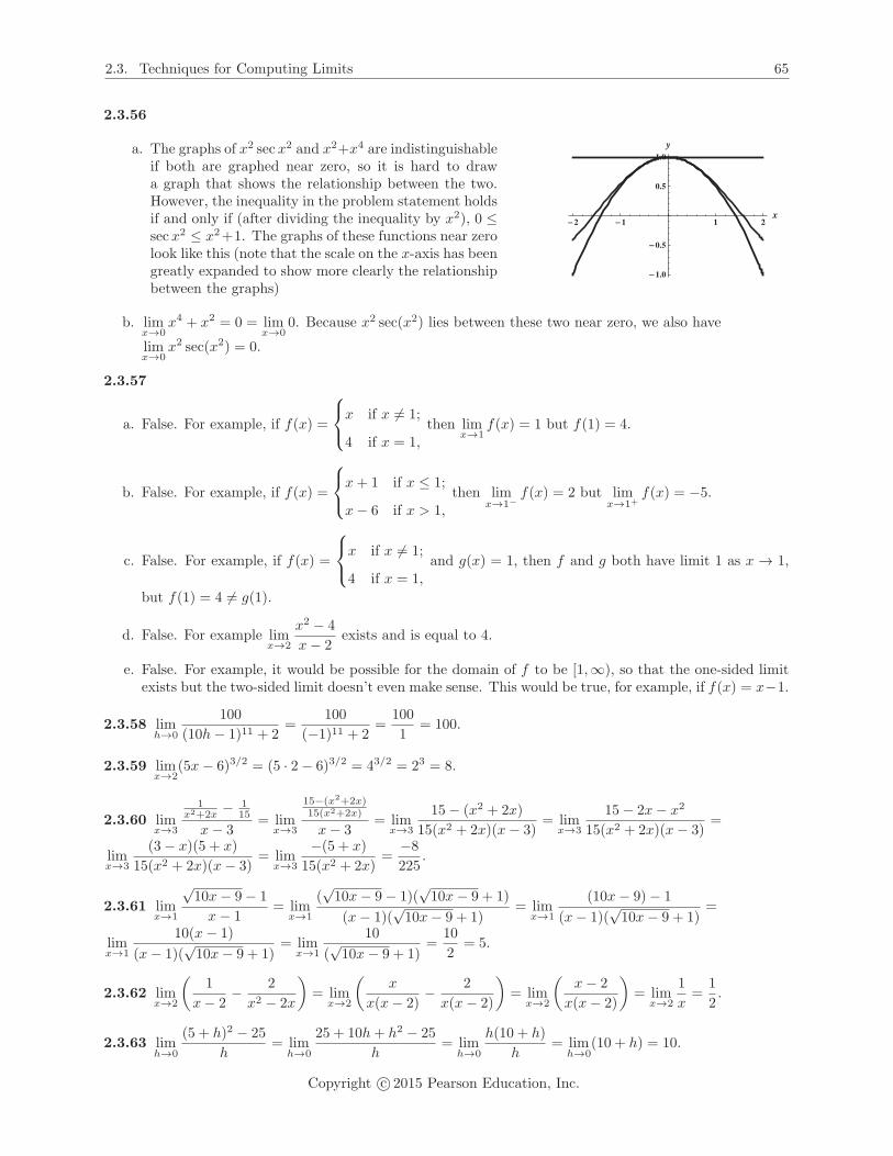
2.3. Techniques for Computing Limits 65
2.3.56
a. The graphs of x2 secx2 and x2+x4 are indistinguishableif both are graphed near zero, so it is hard to drawa graph that shows the relationship between the two.However, the inequality in the problem statement holdsif and only if (after dividing the inequality by x2), 0 ≤secx2 ≤ x2+1. The graphs of these functions near zerolook like this (note that the scale on the x-axis has beengreatly expanded to show more clearly the relationshipbetween the graphs)
�2 �1 1 2x
�1.0
�0.5
0.5
1.0y
b. limx→0
x4 + x2 = 0 = limx→0
0. Because x2 sec(x2) lies between these two near zero, we also have
limx→0
x2 sec(x2) = 0.
2.3.57
a. False. For example, if f(x) =
⎧⎨⎩x if x = 1;
4 if x = 1,then lim
x→1f(x) = 1 but f(1) = 4.
b. False. For example, if f(x) =
⎧⎨⎩x+ 1 if x ≤ 1;
x− 6 if x > 1,then lim
x→1−f(x) = 2 but lim
x→1+f(x) = −5.
c. False. For example, if f(x) =
⎧⎨⎩x if x = 1;
4 if x = 1,and g(x) = 1, then f and g both have limit 1 as x → 1,
but f(1) = 4 = g(1).
d. False. For example limx→2
x2 − 4
x− 2exists and is equal to 4.
e. False. For example, it would be possible for the domain of f to be [1,∞), so that the one-sided limitexists but the two-sided limit doesn’t even make sense. This would be true, for example, if f(x) = x−1.
2.3.58 limh→0
100
(10h− 1)11 + 2=
100
(−1)11 + 2=
100
1= 100.
2.3.59 limx→2
(5x− 6)3/2 = (5 · 2− 6)3/2 = 43/2 = 23 = 8.
2.3.60 limx→3
1x2+2x − 1
15
x− 3= lim
x→3
15−(x2+2x)15(x2+2x)
x− 3= lim
x→3
15− (x2 + 2x)
15(x2 + 2x)(x− 3)= lim
x→3
15− 2x− x2
15(x2 + 2x)(x− 3)=
limx→3
(3− x)(5 + x)
15(x2 + 2x)(x− 3)= lim
x→3
−(5 + x)
15(x2 + 2x)=
−8
225.
2.3.61 limx→1
√10x− 9− 1
x− 1= lim
x→1
(√10x− 9− 1)(
√10x− 9 + 1)
(x− 1)(√10x− 9 + 1)
= limx→1
(10x− 9)− 1
(x− 1)(√10x− 9 + 1)
=
limx→1
10(x− 1)
(x− 1)(√10x− 9 + 1)
= limx→1
10
(√10x− 9 + 1)
=10
2= 5.
2.3.62 limx→2
(1
x− 2− 2
x2 − 2x
)= lim
x→2
(x
x(x− 2)− 2
x(x− 2)
)= lim
x→2
(x− 2
x(x− 2)
)= lim
x→2
1
x=
1
2.
2.3.63 limh→0
(5 + h)2 − 25
h= lim
h→0
25 + 10h+ h2 − 25
h= lim
h→0
h(10 + h)
h= lim
h→0(10 + h) = 10.
Copyright c© 2015 Pearson Education, Inc.

66 Chapter 2. Limits
2.3.64 limx→c
x2 − 2cx+ c2
x− c= lim
x→c
(x− c)2
x− c= lim
x→cx− c = c− c = 0.
2.3.65 We have
limw→−k
w2 + 5kw + 4k2
w2 + kw= lim
w→−k
(w + 4k)(w + k)
(w)(w + k)= lim
w→−k
w + 4k
w=
−k + 4k
−k= −3.
If k = 0, we have limw→−k
w2 + 5kw + 4k2
w2 + kw= lim
w→0
w2
w2= 1.
2.3.66 In order for limx→2
f(x) to exist, we need the two one-sided limits to exist and be equal. We have
limx→2−
f(x) = limx→2−
(3x+ b) = 6 + b, and limx→2+
f(x) = limx→2+
(x− 2) = 0. So we need 6 + b = 0, so we require
that b = −6. Then limx→2
f(x) = 0.
2.3.67 In order for limx→−1
g(x) to exist, we need the two one-sided limits to exist and be equal. We have
limx→−1−
g(x) = limx→−1−
(x2 − 5x) = 6, and limx→−1+
g(x) = limx→−1+
(ax3 − 7) = −a− 7. So we need −a− 7 = 6, so
we require that a = −13. Then limx→−1
f(x) = 6.
2.3.68 limx→2
x5 − 32
x− 2= lim
x→2
(x− 2)(x4 + 2x3 + 4x2 + 8x+ 16)
x− 2= lim
x→2(x4 + 2x3 + 4x2 + 8x+ 16) = 16 + 16 +
16 + 16 + 16 = 80.
2.3.69 limx→1
x6 − 1
x− 1= lim
x→1
(x− 1)(x5 + x4 + x3 + x2 + x+ 1)
x− 1= lim
x→1(x5 + x4 + x3 + x2 + x+ 1) = 6.
2.3.70 limx→−1
x7 + 1
x+ 1= lim
x→−1
(x+ 1)(x6 − x5 + x4 − x3 + x2 − x+ 1)
x+ 1= lim
x→−1(x6 − x5 + x4 − x3 + x2 − x+ 1) = 7.
2.3.71 limx→a
x5 − a5
x− a= lim
x→a
(x− a)(x4 + ax3 + a2x2 + a3x+ a4)
x− a= lim
x→a(x4 + ax3 + a2x2 + a3x+ a4) = 5a4.
2.3.72 limx→a
xn − an
x− a= lim
x→a
(x− a)(xn−1 + axn−2 + · · ·+ an−2x+ an−1)
x− a= lim
x→a(xn−1+axn−2+· · ·+an−2x+
an−1) = nan−1.
2.3.73 limx→1
3√x− 1
x− 1= lim
x→1
3√x− 1
( 3√x− 1)(
3√x2 + 3
√x+ 1)
= limx→1
13√x2 + 3
√x+ 1
=1
3.
2.3.74 limx→16
4√x− 2
x− 16= lim
x→16
4√x− 2
( 4√x− 2)(
4√x3 + 2
4√x2 + 4 4
√x+ 8)
= limx→16
14√x3 + 2
4√x2 + 4 4
√x+ 8
=1
32.
2.3.75 limx→1
x− 1√x− 1
= limx→1
(x− 1)(√x+ 1)
(√x− 1)(
√x+ 1)
= limx→1
(x− 1)(√x+ 1)
x− 1= lim
x→1(√x+ 1) = 2.
2.3.76 limx→1
x− 1√4x+ 5− 3
= limx→1
(x− 1)(√4x+ 5 + 3)
(√4x+ 5− 3)(
√4x+ 5 + 3)
= limx→1
(x− 1)(√4x+ 5 + 3)
4x+ 5− 9=
limx→1
(x− 1)(√4x+ 5 + 3)
4(x− 1)= lim
x→1
(√4x+ 5 + 3)
4=
6
4=
3
2.
2.3.77 limx→43(x−4)
√x+5
3−√x+5
= limx→43(x−4)(
√x+5)(3+
√x+5)
(3−√x+5)(3+
√x+5)
= limx→43(x−4)(
√x+5)(3+
√x+5)
9−(x+5) =
limx→43(x−4)(
√x+5)(3+
√x+5)
−(x−4) = limx→4[−3(√x+ 5)(3 +
√x+ 5)] = (−3)(3)(3 + 3) = −54.
Copyright c© 2015 Pearson Education, Inc.

2.3. Techniques for Computing Limits 67
2.3.78 Assume c = 0. limx→0
x√cx+ 1− 1
= limx→0
x(√cx+ 1 + 1)
(√cx+ 1− 1)(
√cx+ 1 + 1)
= limx→0
x(√cx+ 1 + 1)
(cx+ 1)− 1=
limx→0
x(√cx+ 1 + 1)
cx= lim
x→0
(√cx+ 1 + 1)
c=
2
c.
2.3.79 Let f(x) = x− 1 and g(x) = 5x−1 . Then lim
x→1f(x) = 0, lim
x→1f(x)g(x) = lim
x→1
5(x− 1)
x− 1= lim
x→15 = 5.
2.3.80 Let f(x) = x2 − 1. Then limx→1
f(x)
x− 1= lim
x→1
x2 − 1
x− 1= lim
x→1(x+ 1) = 2.
2.3.81 Let p(x) = x2 + 2x− 8. Then limx→2
p(x)
x− 2= lim
x→2
(x− 2)(x+ 4)
x− 2= lim
x→2(x+ 4) = 6.
The constants are unique. We know that 2 must be a root of p (otherwise the given limit couldn’texist), so it must have the form p(x) = (x − 2)q(x), and q must be a degree 1 polynomial with leadingcoefficient 1 (otherwise p wouldn’t have leading coefficient 1.) So we have p(x) = (x− 2)(x+ d), but because
limx→2
p(x)
x− 2= lim
x→2(x + d) = 2 + d = 6, we are forced to realize that d = 4. Therefore, we have deduced that
the only possibility for p is p(x) = (x− 2)(x+ 4) = x2 + 2x− 8.
2.3.82
a. L(c/2) = L0
√1− (c/2)2
c2 = L0
√1− (1/4) =
√3L0/2.
b. L(3c/4) = L0
√1− (1/c2)(3c/4)2 = L0
√1− (9/16) =
√7L0/4.
c. It appears that that the observed length L of the ship decreases as the ship speed increases.
d. limx→c−
L0
√1− (ν2/c2) = L0 ·0 = 0. As the speed of the ship approaches the speed of light, the observed
length of the ship shrinks to 0.
2.3.83 limS→0+
r(S) = limS→0+
(1/2)
(√100 +
2S
π− 10
)= 0.
The radius of the circular cylinder approaches zero as the surface area approaches zero.
2.3.84 limt→200−
d(t) = limt→200−
(3 − 0.015t)2 = (3 − (0.015)(200))2 = (3 − 3)2 = 0. As time approaches 200
seconds, the depth of the water in the tank is approaching 0.
2.3.85 limx→10
E(x) = limx→10
4.35
x√x2 + 0.01
=4.35
10√100.01
≈ .0435 N/C.
2.3.86 Because limx→1
f(x) = 4, we know that f is near 4 when x is near 1 (but not equal to 1). It follows
that limx→−1
f(x2) = 4 as well, because when x is near but not equal to −1, x2 is near 1 but not equal to 1.
Thus f(x2) is near 4 when x is near −1.
2.3.87
a. As x → 0+, (1− x) → 1−. So limx→0+
g(x) = lim(1−x)→1−
f(1− x) = limz→1−
f(z) = 6. (Where z = 1− x.)
b. As x → 0−, (1− x) → 1+. So limx→0−
g(x) = lim(1−x)→1+
f(1− x) = limz→1+
f(z) = 4. (Where z = 1− x.)
2.3.88
a. Suppose 0 < θ < π/2. Note that sin θ > 0, so | sin θ| = sin θ. Also, sin θ = |AC|1 , so |AC| = | sin θ|.
Now suppose that −π/2 < θ < 0. Then sin θ is negative, so | sin θ| = − sin θ. We have sin θ = −|AC|1 ,
so |AC| = − sin θ = | sin θ|.
Copyright c© 2015 Pearson Education, Inc.

68 Chapter 2. Limits
b. Suppose 0 < θ < π/2. Because AB is the hypotenuse of triangle ABC, we know that |AB| > |AC|.We have | sin θ| = |AC| < |AB| < the length of arc AB = θ = |θ|.If −π/2 < θ < 0, we can make a similar argument. We have
| sin θ| = |AC| < |AB| < the length of arc AB = −θ = |θ|.
c. If 0 < θ < π/2, we have sin θ = | sin θ| < |θ|, and because sin θ is positive, we have −|θ| ≤ 0 < sin θ.Putting these together gives −|θ| < sin θ < |θ|.If −π/2 < θ < 0, then | sin θ| = − sin θ. From the previous part, we have | sin θ| = − sin θ < |θ|.Therefore, −|θ| < sin θ. Now because sin θ is negative on this interval, we have sin θ < 0 ≤ |θ|. Puttingthese together gives −|θ| < sin θ < |θ|.
d. If 0 < θ < π/2, we have
0 ≤ 1− cos θ = |OB| − |OC| = |BC| < |AB| < the length of arc AB = θ = |θ|.
For −π/2 < θ < 0, we have
0 ≤ 1− cos θ = |OB| − |OC| = |BC| < |AB| < the length of arc AB = −θ = |θ|.
2.3.89 limx→a
p(x) = limx→a
(anxn+an−1x
n−1+ · · ·+a1x+a0) = limx→a
(anxn)+ lim
x→a(an−1x
n−1)+ · · ·+ limx→a
(a1x)+
limx→a
a0 = an limx→a
xn+an−1 limx→a
xn−1+· · ·+a1 limx→a
x+a0 = an( limx→a
x)n+an−1( limx→a
x)n−1+· · ·+a1( limx→a
x)+a0 =
anan + an−1a
n−1 + · · ·+ a1a+ a0 = p(a).
2.4 Infinite Limits
2.4.1
limx→a+
f(x) = −∞ means that when x is very close
to (but a little bigger than) a, the correspondingvalues for f(x) are negative numbers whose abso-lute value is very large.
ax
y
2.4.2
limx→a
f(x) = ∞ means that when x is close to (but
not equal to) a, the corresponding values for f(x)are very large positive numbers.
y � f �x�
ax
y
2.4.3 A vertical asymptote for a function f is a vertical line x = a so that one or more of the following aretrue: lim
x→a−f(x) = ±∞, lim
x→a+f(x) = ±∞.
Copyright c© 2015 Pearson Education, Inc.

2.4. Infinite Limits 69
2.4.4 No. For example, if f(x) = x2 − 4 and g(x) = x − 2 and a = 2, we would have limx→2
f(x)
g(x)= 4, even
though g(2) = 0.
2.4.5 Because the numerator is approaching a non-zero constant while the denominator is approaching zero,the quotient of these numbers is getting big – at least the absolute value of the quotient is getting big. Thequotient is actually always negative, because a number near 100 divided by a negative number is always
negative. Thus limx→2
f(x)
g(x)= −∞.
2.4.6 Using the same sort of reasoning as in the last problem – as x → 3 the numerator is fixed at 1, butthe denominator is getting small, so the quotient is getting big. It remains to investigate the sign of thequotient. As x → 3−, the quantity x− 3 is negative, so the quotient of the positive number 1 and this smallnegative number is negative. On the other hand, as x → 3+, the quantity x− 3 is positive, so the quotient
of 1 and this number is positive. Thus: limx→3−
1
x− 3= −∞, and lim
x→3+
1
x− 3= ∞.
2.4.7
x x+1(x−1)2 x x+1
(x−1)2
1.1 210 .9 190
1.01 20,100 .99 19,900
1.001 2,001,000 .999 1,999,000
1.0001 200,010,000 .9999 199,990,000
From the data given, it appears that limx→1
f(x) = ∞.
2.4.8 limx→3
f(x) = ∞, and limx→−1
f(x) = −∞.
2.4.9
a. limx→1−
f(x) = ∞. b. limx→1+
f(x) = ∞. c. limx→1
f(x) = ∞.
d. limx→2−
f(x) = ∞. e. limx→2+
f(x) = −∞. f. limx→2
f(x) does not exist.
2.4.10
a. limx→2−
g(x) = ∞. b. limx→2+
g(x) = −∞. c. limx→2
g(x) does not exist.
d. limx→4−
g(x) = −∞. e. limx→4+
g(x) = −∞. f. limx→4
g(x) = −∞.
2.4.11
a. limx→−2−
h(x) = −∞. b. limx→−2+
h(x) = −∞. c. limx→−2
h(x) = −∞.
d. limx→3−
h(x) = ∞. e. limx→3+
h(x) = −∞. f. limx→3
h(x) does not exist.
2.4.12
a. limx→−2−
p(x) = −∞. b. limx→−2+
p(x) = −∞. c. limx→−2
p(x) = −∞.
d. limx→3−
p(x) = −∞. e. limx→3+
p(x) = −∞. f. limx→3
p(x) = −∞.
Copyright c© 2015 Pearson Education, Inc.

70 Chapter 2. Limits
2.4.13
a. limx→0−
1
x2 − x= ∞.
b. limx→0+
1
x2 − x= −∞.
c. limx→1−
1
x2 − x= −∞.
d. limx→1+
1
x2 − x= ∞.
0 1 x
2.4.14
a. limx→π+
x cotx = ∞.
b. limx→π−
x cotx = −∞.
c. limx→−π+
x cotx = −∞.
d. limx→−π−
x cotx = ∞.
�4 �2 2 4 x
�10
�5
5
10
15
y
2.4.15
1 2 3 4 x
�4
�2
2
4
y
2.4.16
2 4 6 8 x
�5
5
y
2.4.17
a. limx→2+
1
x− 2= ∞. b. lim
x→2−
1
x− 2= −∞. c. lim
x→2
1
x− 2does not exist.
2.4.18
a. limx→3+
2
(x− 3)3= ∞. b. lim
x→3−
2
(x− 3)3= −∞. c. lim
x→3
2
(x− 3)3does not exist.
2.4.19
a. limx→4+
x− 5
(x− 4)2= −∞. b. lim
x→4−
x− 5
(x− 4)2= −∞. c. lim
x→4
x− 5
(x− 4)2= −∞.
2.4.20
a. limx→1+
x− 2
(x− 1)3= −∞. b. lim
x→1−
x− 2
(x− 1)3= ∞. c. lim
x→1
x− 2
(x− 1)3does not exist.
Copyright c© 2015 Pearson Education, Inc.

2.4. Infinite Limits 71
2.4.21
a. limx→3+
(x− 1)(x− 2)
(x− 3)= ∞. b. lim
x→3−
(x− 1)(x− 2)
(x− 3)= −∞. c. lim
x→3
(x− 1)(x− 2)
(x− 3)does not exist.
2.4.22
a. limx→−2+
(x− 4)
x(x+ 2)= ∞. b. lim
x→−2−
(x− 4)
x(x+ 2)= −∞. c. lim
x→−2
(x− 4)
x(x+ 2)does not exist.
2.4.23
a. limx→2+
x2 − 4x+ 3
(x− 2)2= −∞. b. lim
x→2−
x2 − 4x+ 3
(x− 2)2= −∞. c. lim
x→2
x2 − 4x+ 3
(x− 2)2= −∞.
2.4.24
a. limx→−2+
x3 − 5x2 + 6x
x4 − 4x2= lim
x→−2+
x(x− 2)(x− 3)
x2(x− 2)(x+ 2)= lim
x→−2+
x− 3
x(x+ 2)= ∞.
b. limx→−2−
x3 − 5x2 + 6x
x4 − 4x2= lim
x→−2−
x(x− 2)(x− 3)
x2(x− 2)(x+ 2)= lim
x→−2−
x− 3
x(x+ 2)= −∞.
c. Because the two one-sided limits differ, limx→−2
x3 − 5x2 + 6x
x4 − 4x2does not exist.
d. limx→2
x3 − 5x2 + 6x
x4 − 4x2= lim
x→2
x− 3
x(x+ 2)=
−1
8.
2.4.25 limx→0
x3 − 5x2
x2= lim
x→0
x2(x− 5)
x2= lim
x→0(x− 5) = −5.
2.4.26 limt→5
4t2 − 100
t− 5= lim
t→5
4(t− 5)(t+ 5)
t− 5= lim
t→5[4(t+ 5)] = 40.
2.4.27 limx→1+
x2 − 5x+ 6
x− 1= lim
x→1+
(x− 2)(x− 3)
x− 1= ∞. (Note that as x → 1+, the numerator is near 2, while
the denominator is near zero, but is positive. So the quotient is positive and large.)
2.4.28 limz→4
z − 5
(z2 − 10z + 24)2= lim
z→4
z − 5
(z − 4)2(z − 6)2= −∞. (Note that as z → 4, the numerator is near −1
while the denominator is near zero but is positive. So the quotient is negative with large absolute value.)
2.4.29
a. limx→5
x− 5
x2 − 25= lim
x→5
1
x+ 5=
1
10, so there isn’t a vertical asymptote at x = 5.
b. limx→−5−
x− 5
x2 − 25= lim
x→−5−
1
x+ 5= −∞, so there is a vertical asymptote at x = −5.
c. limx→−5+
x− 5
x2 − 25= lim
x→−5+
1
x+ 5= ∞. This also implies that x = −5 is a vertical asymptote, as we
already noted in part b.
2.4.30
a. limx→7−
x+ 7
x4 − 49x2= lim
x→7−
x+ 7
x2(x+ 7)(x− 7)= lim
x→7−
1
x2(x− 7)= −∞, so there is a vertical asymptote
at x = 7.
Copyright c© 2015 Pearson Education, Inc.

72 Chapter 2. Limits
b. limx→7+
x+ 7
x4 − 49x2= lim
x→7+
x+ 7
x2(x+ 7)(x− 7)= lim
x→7+
1
x2(x− 7)= ∞. This also implies that there is a
vertical asymptote at x = 7, as we already noted in part a.
c. limx→−7
x+ 7
x4 − 49x2= lim
x→−7
x+ 7
x2(x+ 7)(x− 7)= lim
x→−7
1
x2(x− 7)=
1
−686. So there is not a vertical
asymptote at x = 7.
d. limx→0
x+ 7
x4 − 49x2= lim
x→0
x+ 7
x2(x+ 7)(x− 7)= lim
x→0
1
x2(x− 7)= −∞. So there is a vertical asymptote at
x = 0.
2.4.31 f(x) = x2−9x+14x2−5x+6 = (x−2)(x−7)
(x−2)(x−3) . Note that x = 3 is a vertical asymptote, while x = 2 appears to be
a candidate but isn’t one. We have limx→3+
f(x) = limx→3+
x− 7
x− 3= −∞ and lim
x→3−f(x) = lim
x→3−
x− 7
x− 3= ∞, and
thus limx→3
f(x) doesn’t exist. Note that limx→2
f(x) = 5.
2.4.32 f(x) = cos xx(x+2) has vertical asymptotes at x = 0 and at x = −2. Note that cosx is near 1 when x is
near 0 , and cosx is near −.4 when x is near −2. Thus, limx→0+
f(x) = +∞, limx→0−
f(x) = −∞, limx→−2+
f(x) = ∞,
and limx→−2−
f(x) = −∞.
2.4.33 f(x) = x+1x3−4x2+4x = x+1
x(x−2)2 . There are vertical asymptotes at x = 0 and x = 2. We have
limx→0−
f(x) = limx→0−
x+ 1
x(x− 2)2= −∞, while lim
x→0+f(x) = lim
x→0+
x+ 1
x(x− 2)2= ∞, and thus lim
x→0f(x) doesn’t
exist.
Also we have limx→2−
f(x) = limx→2−
x+ 1
x(x− 2)2= ∞, while lim
x→2+f(x) = lim
x→2+
x+ 1
x(x− 2)2= ∞, and thus
limx→2
f(x) = ∞ as well.
2.4.34 g(x) = x3−10x2+16xx2−8x = x(x−2)(x−8)
x(x−8) . This function has no vertical asymptotes.
2.4.35 limθ→0+
csc θ = limθ→0+
1
sin θ= ∞.
2.4.36 limx→0−
cscx = limx→0−
1
sinx= −∞.
2.4.37 limx→0+
−10 cotx = limx→0+
−10 cosx
sinx= −∞. (Note that as x → 0+, the numerator is near −10 and the
denominator is near zero, but is positive. Thus the quotient is a negative number whose absolute value islarge.)
2.4.38 limθ→(π/2)+
1
3tan θ = lim
θ→(π/2)+
sin θ
3 cos θ= −∞. (Note that as θ → (π/2)+, the numerator is near 1 and
the denominator is near 0, but is negative. Thus the quotient is a negative number whose absolute value islarge.)
2.4.39
a. limx→(π/2)+
tanx = −∞.
b. limx→(π/2)−
tanx = ∞.
c. limx→(−π/2)+
tanx = −∞.
d. limx→(−π/2)−
tanx = ∞.
�3 �2 �1 1 2 3 x
�10
�5
5
10y
Copyright c© 2015 Pearson Education, Inc.

2.4. Infinite Limits 73
2.4.40
a. limx→(π/2)+
secx tanx = ∞.
b. limx→(π/2)−
secx tanx = ∞.
c. limx→(−π/2)+
secx tanx = −∞.
d. limx→(−π/2)−
secx tanx = −∞.
�3 �2 �1 1 2 3 x
�10
�5
5
10y
2.4.41
a. False. limx→1−
f(x) = limx→1+
f(x) = limx→1
f(x) = limx→1
(x− 1)(x− 6)
(x− 1)(x+ 1)=
−5
2.
b. True. For example, limx→−1+
f(x) = limx→−1+
(x− 1)(x− 6)
(x− 1)(x+ 1)= −∞.
c. False. For example g(x) = 1x−1 has lim
x→1+g(x) = ∞, but lim
x→1−g(x) = −∞.
2.4.42
One such function is f(x) = x2−4x+3x2−3x+2 =
(x−1)(x−3)(x−1)(x−2) .
�1 1 2 3 x
�4
�2
2
4
6
y
2.4.43 One example is f(x) = 1x−6 .
2.4.44function a b c d e f
graph D C F B A E
2.4.45 f(x) = x2−3x+2x10−x9 = (x−2)(x−1)
x9(x−1) . f has a vertical asymptote at x = 0, because limx→0+
f(x) = −∞ (and
limx→0−
f(x) = ∞.) Note that limx→1
f(x) = −1, so there isn’t a vertical asymptote at x = 1.
2.4.46 g(x) = cot(x− π
2
)has vertical asymptotes at x = ±π
2, because lim
x→π/2−cot(x− π
2
)= −∞, and
limx→−π/2+
cot(x− π
2
)= ∞.
2.4.47 h(x) =cosx
(x+ 1)3has a vertical asymptote at x = −1, because lim
x→−1+
cosx
(x+ 1)3= ∞, and because
limx→−1−
h(x) = −∞.
2.4.48 p(x) = sec(πx/2) = 1cos(πx/2) has a vertical asymptote on (−2, 2) at x = ±1.
Copyright c© 2015 Pearson Education, Inc.

74 Chapter 2. Limits
2.4.49 g(θ) = tan(πθ/10) = sin(πθ/10)cos(πθ/10) has a vertical asymptote at each θ = 10n + 5 where n is an integer.
This is due to the fact that cos(πθ/10) = 0 when πθ/10 = π/2+nπ where n is an integer, which is the sameas {θ : θ = 10n+ 5, n an integer}. Note that at all of these numbers which make the denominator zero, thenumerator isn’t zero.
2.4.50 q(s) = πs−sin s has a vertical asymptote at s = 0. Note that this is the only number where sin s = s.
2.4.51 f(x) = 1√x sec x
= cos x√x
has a vertical asymptote at x = 0.
2.4.52 Note that g(x) is defined only when x(x2−1) > 0, i.e. for x ∈ (−1, 0)∪(1,∞). Then limx→−1+
g(x) = ∞,
limx→0−
g(x) = ∞, limx→1+
g(x) = ∞, so that g(x) has vertical asymptotes for x = ±1, 0.
2.4.53
a. Note that the numerator of the given expression factors as (x− 3)(x− 4). So if a = 3 or if a = 4 the
limit would be a finite number. In fact, limx→3
(x− 3)(x− 4)
x− 3= −1 and lim
x→4
(x− 3)(x− 4)
x− 4= 1.
b. For any number other than 3 or 4, the limit would be either ±∞. Because x − a is always positiveas x → a+, the limit would be +∞ exactly when the numerator is positive, which is for a in the set(−∞, 3) ∪ (4,∞).
c. The limit would be −∞ for a in the set (3, 4).
2.4.54
a. The slope of the secant line is given by f(h)−f(0)h = h1/3
h = h−2/3.
b. limh→0
13√h2
= ∞. This tells us that the slope of the tangent line is infinite – which means that the
tangent line at (0, 0) is vertical.
2.4.55
a. The slope of the secant line is f(h)−f(0)h = h2/3
h = h−1/3.
b. limh→0+
1
h1/3= ∞, and lim
h→0−
1
h1/3= −∞. The tangent line is infinitely steep at the origin (i.e., it is a
vertical line.)
2.5 Limits at Infinity
2.5.1
As x < 0 becomes large in absolute value, thecorresponding values of f level off near 10.
x
10y
2.5.2 A horizontal asymptote is a horizontal line y = L so that either limx→∞ f(x) = L or lim
x→−∞ f(x) = L (or
both.)
Copyright c© 2015 Pearson Education, Inc.

2.5. Limits at Infinity 75
2.5.3 If f(x) → 100, 000 as x → ∞ and g(x) → ∞ as x → ∞, then the ratio f(x)g(x) → 0 as x → ∞. (Because
eventually the values of f are small compared to the values of g.)
2.5.4 As x → ±∞, sinx remains between −1 and 1, so that limx→∞ g(x) = 0 and limx→−∞ g(x) = 0.
2.5.5 limx→∞(−2x3) = −∞, and lim
x→−∞(−2x3) = ∞.
2.5.6 The line y = 0 may be a horizontal asymptote, the line y = a where a = 0 may be a horizontalasymptote, and the limit at ±∞ may not exist either with or without a slant asymptote.
2.5.7
limx→∞
1− x
2x= −1
2, lim
x→∞1− x
x2= 0, lim
x→∞1− x2
2x= −∞
2.5.8
As x → ∞ (or as x → −∞), cosx oscillates between −1and 1. Thus neither lim
x→∞ cosx nor limx→−∞ cosx exists. x
y
�0.5
0.5
1.0
�1.0
�5�10 5 10
2.5.9 limx→∞(3 + 10/x2) = 3 + lim
x→∞(10/x2) = 3 + 0 = 3.
2.5.10 limx→∞(5 + 1/x+ 10/x2) = 5 + lim
x→∞(1/x) + limx→∞(10/x2) = 5 + 0 + 0 = 5.
2.5.11 limθ→∞
cos θ
θ2= 0. Note that −1 ≤ cos θ ≤ 1, so − 1
θ2 ≤ cos θθ2 ≤ 1
θ2 . The result now follows from the
squeeze theorem.
2.5.12 limx→∞
3 + 2x+ 4x2
x2= lim
x→∞3
x2+ lim
x→∞2x
x2+ lim
x→∞4x2
x2= 0 + lim
x→∞2
x+ lim
x→∞ 4 = 0 + 0 + 4 = 4.
2.5.13 limx→∞
cosx5
√x
= 0. Note that −1 ≤ cosx5 ≤ 1, so −1√x≤ cos x5√
x≤ 1√
x. Because lim
x→∞1√x= lim
x→∞−1√x=
0, we have limx→∞
cosx5
√x
= 0 by the squeeze theorem.
2.5.14 limx→−∞
(5 +
100
x+
sin4(x3)
x2
)= 5 + 0 + 0 = 5. For this last limit, note that 0 ≤ sin4(x3) ≤ 1, so
0 ≤ sin4(x3)x2 ≤ 1
x2 . The result now follows from the squeeze theorem.
2.5.15 limx→∞x12 = ∞. Note that x12 is positive when x > 0.
2.5.16 limx→−∞ 3x11 = −∞. Note that x11 is negative when x < 0.
Copyright c© 2015 Pearson Education, Inc.

76 Chapter 2. Limits
2.5.17 limx→∞x−6 = lim
x→∞1
x6= 0.
2.5.18 limx→−∞x−11 = lim
x→−∞1
x11= 0.
2.5.19 limx→∞(3x12 − 9x7) = ∞.
2.5.20 limx→−∞(3x7 + x2) = −∞.
2.5.21 limx→−∞(−3x16 + 2) = −∞.
2.5.22 limx→−∞ 2x−8 = lim
x→−∞2
x8= 0.
2.5.23 limx→∞(−12x−5) = lim
x→∞−12
x5= 0.
2.5.24 limx→−∞(2x−8 + 4x3) = 0 + lim
x→−∞ 4x3 = −∞.
2.5.25 limx→∞
4x
20x+ 1= lim
x→∞4x
20x+ 1· 1/x1/x
= limx→∞
4
20 + 1/x=
4
20=
1
5. Thus, the line y = 1
5 is a horizontal
asymptote.
limx→−∞
4x
20x+ 1= lim
x→−∞4x
20x+ 1· 1/x1/x
= limx→−∞
4
20 + 1/x=
4
20=
1
5. This shows that the curve is also
asymptotic to the asymptote in the negative direction.
2.5.26 limx→∞
3x2 − 7
x2 + 5x= lim
x→∞3x2 − 7
x2 + 5x· 1/x
2
1/x2= lim
x→∞3− (7/x2)
1 + (5/x)=
3− 0
1 + 0= 3. Thus, the line y = 3 is a
horizontal asymptote.
limx→−∞
3x2 − 7
x2 + 5x= lim
x→−∞3x2 − 7
x2 + 5x· 1/x
2
1/x2= lim
x→−∞3− (7/x2)
1 + (5/x)=
3− 0
1 + 0= 3. Thus, the curve is also
asymptotic to the asymptote in the negative direction.
2.5.27 limx→∞
(6x2 − 9x+ 8)
(3x2 + 2)· 1/x
2
1/x2= lim
x→∞6− 9/x+ 8/x2
3 + 2/x2=
6− 0 + 0
3 + 0= 2. Similarly lim
x→−∞ f(x) = 2. The
line y = 2 is a horizontal asymptote.
2.5.28 limx→∞
(4x2 − 7)
(8x2 + 5x+ 2)· 1/x
2
1/x2= lim
x→∞4− 7/x2
8 + 5/x+ 2/x2=
4− 0
8 + 0 + 0=
1
2. Similarly lim
x→−∞ f(x) =1
2. The
line y = 12 is a horizontal asymptote.
2.5.29 limx→∞
3x3 − 7
x4 + 5x2= lim
x→∞3x3 − 7
x4 + 5x2· 3/x
4
1/x4= lim
x→∞1/x− (7/x4)
1 + (5/x2)=
0− 0
1 + 0= 0. Thus, the line y = 0 (the
x-axis) is a horizontal asymptote.
limx→−∞
3x3 − 7
x4 + 5x2= lim
x→−∞3x3 − 7
x4 + 5x2· 3/x
4
1/x4= lim
x→−∞1/x− (7/x4)
1 + (5/x2)=
0− 0
1 + 0= 0. Thus, the curve is
asymptotic to the x-axis in the negative direction as well.
2.5.30 limx→∞
x4 + 7
x5 + x2 − x= lim
x→∞x4 + 7
x5 + x2 − x· 1/x
5
1/x5= lim
x→∞(1/x) + (7/x5)
1 + (1/x3)− (1/x4)=
0 + 0
1 + 0− 0= 0. Thus, the
line y = 0 (the x-axis) is a horizontal asymptote.
limx→−∞
x4 + 7
x5 + x2 − x= lim
x→−∞x4 + 7
x5 + x2 − x· 1/x
5
1/x5= lim
x→−∞(1/x) + (7/x5)
1 + (1/x3)− (1/x4)=
0 + 0
1 + 0− 0= 0. Thus, the
curve is asymptotic to the x-axis in the negative direction as well.
Copyright c© 2015 Pearson Education, Inc.
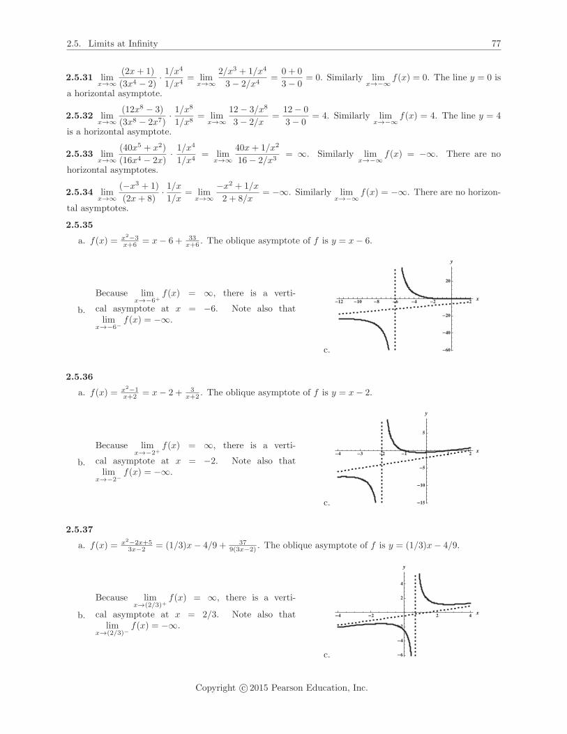
2.5. Limits at Infinity 77
2.5.31 limx→∞
(2x+ 1)
(3x4 − 2)· 1/x
4
1/x4= lim
x→∞2/x3 + 1/x4
3− 2/x4=
0 + 0
3− 0= 0. Similarly lim
x→−∞ f(x) = 0. The line y = 0 is
a horizontal asymptote.
2.5.32 limx→∞
(12x8 − 3)
(3x8 − 2x7)· 1/x
8
1/x8= lim
x→∞12− 3/x8
3− 2/x=
12− 0
3− 0= 4. Similarly lim
x→−∞ f(x) = 4. The line y = 4
is a horizontal asymptote.
2.5.33 limx→∞
(40x5 + x2)
(16x4 − 2x)· 1/x
4
1/x4= lim
x→∞40x+ 1/x2
16− 2/x3= ∞. Similarly lim
x→−∞ f(x) = −∞. There are no
horizontal asymptotes.
2.5.34 limx→∞
(−x3 + 1)
(2x+ 8)· 1/x1/x
= limx→∞
−x2 + 1/x
2 + 8/x= −∞. Similarly lim
x→−∞ f(x) = −∞. There are no horizon-
tal asymptotes.
2.5.35
a. f(x) = x2−3x+6 = x− 6 + 33
x+6 . The oblique asymptote of f is y = x− 6.
b.
Because limx→−6+
f(x) = ∞, there is a verti-
cal asymptote at x = −6. Note also thatlim
x→−6−f(x) = −∞.
c.
�12 �10 �8 �6 �4 �2 2 x
�60
�40
�20
20
y
2.5.36
a. f(x) = x2−1x+2 = x− 2 + 3
x+2 . The oblique asymptote of f is y = x− 2.
b.
Because limx→−2+
f(x) = ∞, there is a verti-
cal asymptote at x = −2. Note also thatlim
x→−2−f(x) = −∞.
c.
�4 �3 �2 �1 1 2 x
�15
�10
�5
5
y
2.5.37
a. f(x) = x2−2x+53x−2 = (1/3)x− 4/9 + 37
9(3x−2) . The oblique asymptote of f is y = (1/3)x− 4/9.
b.
Because limx→(2/3)+
f(x) = ∞, there is a verti-
cal asymptote at x = 2/3. Note also thatlim
x→(2/3)−f(x) = −∞.
c.
�4 �2 2 4 x
�6
�4
�2
2
4
y
Copyright c© 2015 Pearson Education, Inc.

78 Chapter 2. Limits
2.5.38
a. f(x) = 3x2−2x+72x−5 = (3/2)x+ 11/4 + 83
4(2x−5) . The oblique asymptote of f is y = (3/2)x+ 11/4.
b.
Because limx→(5/2)+
f(x) = ∞, there is a verti-
cal asymptote at x = 5/2. Note also thatlim
x→(5/2)−f(x) = −∞.
c.
1 2 3 4 x
�20
20
40
y
2.5.39
a. f(x) = 4x3+4x2+7x+41+x2 = 4x+ 4 + 3x
1+x2 . The oblique asymptote of f is y = 4x+ 4.
b. There are no vertical asymptotes.
c.
�3 �2 �1 1 2 3 x
�5
5
10
15
y
2.5.40
a. f(x) = 3x2−2x+53x+4 = x− 2 + 13
3x+4 . The oblique asymptote of f is y = x− 2.
b.
Because limx→(−4/3)+
f(x) = ∞, there is a verti-
cal asymptote at x = −4/3. Note also thatlim
x→(−4/3)−f(x) = −∞.
c.
�4 �2 2 4 x
�15
�10
�5
5
10
y
2.5.41 First note that√x6 = x3 if x > 0, but
√x6 = −x3 if x < 0. We have lim
x→∞4x3 + 1
(2x3 +√16x6 + 1)
·1/x3
1/x3=
limx→∞
4 + 1/x3
2 +√
16 + 1/x6=
4 + 0
2 +√16 + 0
=2
3.
However, limx→−∞
4x3 + 1
(2x3 +√16x6 + 1)
· 1/x3
1/x3= lim
x→−∞4 + 1/x3
2−√16 + 1/x6=
4 + 0
2−√16 + 0
=4
−2= −2.
So y = 23 is a horizontal asymptote (as x → ∞) and y = −2 is a horizontal asymptote (as x → −∞).
2.5.42 First note that√x2 = x for x > 0, while
√x2 = −x for x < 0. Then lim
x→∞ f(x) can be written as
limx→∞
√x2 + 1
2x+ 1· 1/
√x2
1/x= lim
x→∞
√1 + 1/x2
2 + 1/x=
1
2.
Copyright c© 2015 Pearson Education, Inc.
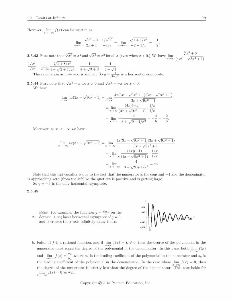
2.5. Limits at Infinity 79
However, limx→−∞ f(x) can be written as
limx→−∞
√x2 + 1
2x+ 1· 1/
√x2
−1/x= lim
x→−∞
√1 + 1/x2
−2− 1/x= −1
2.
2.5.43 First note that3√x6 = x2 and
√x4 = x2 for all x (even when x < 0.) We have lim
x→∞
3√x6 + 8
(4x2 +√3x4 + 1)
·1/x2
1/x2= lim
x→∞
3√1 + 8/x6
4 +√3 + 1/x4
=1
4 +√3 + 0
=1
4 +√3.
The calculation as x → −∞ is similar. So y = 14+
√3is a horizontal asymptote.
2.5.44 First note that√x2 = x for x > 0 and
√x2 = −x for x < 0.
We have
limx→∞ 4x(3x−
√9x2 + 1) = lim
x→∞4x(3x−√
9x2 + 1)(3x+√9x2 + 1)
3x+√9x2 + 1
= limx→∞
(4x)(−1)
(3x+√9x2 + 1)
· 1/x1/x
= limx→∞− 4
3 +√9 + 1/x2
= −4
6= −2
3.
Moreover, as x → −∞ we have
limx→−∞ 4x(3x−
√9x2 + 1) = lim
x→−∞4x(3x−√
9x2 + 1)(3x+√9x2 + 1)
3x+√9x2 + 1
= limx→−∞
(4x)(−1)
(3x+√9x2 + 1)
· 1/x1/x
= limx→−∞− 4
3−√9 + 1/x2= ∞.
Note that this last equality is due to the fact that the numerator is the constant −4 and the denominatoris approaching zero (from the left) so the quotient is positive and is getting large.
So y = − 23 is the only horizontal asymptote.
2.5.45
a.False. For example, the function y = sin x
x on thedomain [1,∞) has a horizontal asymptote of y = 0,and it crosses the x-axis infinitely many times.
10 20 30 40 50x
�0.10
�0.05
0.05
0.10
y
b. False. If f is a rational function, and if limx→∞ f(x) = L = 0, then the degree of the polynomial in the
numerator must equal the degree of the polynomial in the denominator. In this case, both limx→∞ f(x)
and limx→−∞ f(x) =
anbn
where an is the leading coefficient of the polynomial in the numerator and bn is
the leading coefficient of the polynomial in the denominator. In the case where limx→∞ f(x) = 0, then
the degree of the numerator is strictly less than the degree of the denominator. This case holds forlim
x→−∞ f(x) = 0 as well.
Copyright c© 2015 Pearson Education, Inc.

80 Chapter 2. Limits
c. True. There are only two directions which might lead to horizontal asymptotes: there could be one asx → ∞ and there could be one as x → −∞, and those are the only possibilities.
2.5.46
a. limx→∞
x2 − 4x+ 3
x− 1= ∞, and lim
x→−∞x2 − 4x+ 3
x− 1= −∞. There are no horizontal asymptotes.
b. It appears that x = 1 is a candidate to be a vertical asymptote, but note that f(x) = x2−4x+3x−1 =
(x−1)(x−3)x−1 . Thus lim
x→1f(x) = lim
x→1(x− 3) = −2. So f has no vertical asymptotes.
2.5.47
a. limx→∞
2x3 + 10x2 + 12x
x3 + 2x2· (1/x
3)
(1/x3)= lim
x→∞2 + 10/x+ 12/x2
1 + 2/x= 2. Similarly, lim
x→−∞ f(x) = 2. Thus, y = 2
is a horizontal asymptote.
b. Note that f(x) = 2x(x+2)(x+3)x2(x+2) . So lim
x→0+f(x) = lim
x→0+
2(x+ 3)
x= ∞, and similarly, lim
x→0−f(x) = −∞.
There is a vertical asymptote at x = 0. Note that there is no asymptote at x = −2 because limx→−2
f(x) =
−1.
2.5.48
a. We have limx→∞
√16x4 + 64x2 + x2
2x2 − 4· (1/x
2)
(1/x2)= lim
x→∞
√16 + 64/x2 + 1
2− 4/x2=
5
2. Similarly, lim
x→−∞ f(x) =5
2.
So y = 52 is a horizontal asymptote.
b. limx→√
2+f(x) = lim
x→−√2−f(x) = ∞, and lim
x→√2−f(x) = lim
x→−√2+f(x) = −∞ so there are vertical asymp-
totes at x = ±√2.
2.5.49
a. We have limx→∞
3x4 + 3x3 − 36x2
x4 − 25x2 + 144· (1/x
4)
(1/x4)= lim
x→∞3 + 3/x− 36/x2
1− 25/x2 + 144/x4= 3. Similarly, lim
x→−∞ f(x) = 3.
So y = 3 is a horizontal asymptote.
b. Note that f(x) = 3x2(x+4)(x−3)(x+4)(x−4)(x+3)(x−3) . Thus, lim
x→−3+f(x) = −∞ and lim
x→−3−f(x) = ∞. Also,
limx→4−
f(x) = −∞ and limx→4+
f(x) = ∞. Thus there are vertical asymptotes at x = −3 and x = 4.
2.5.50
a. First note that
f(x) = 16x2(4x2 −√
16x4 + 1) · 4x2 +
√16x4 + 1
4x2 +√16x4 + 1
= − 16x2
4x2 +√16x4 + 1
.
We have limx→∞− 16x2
4x2 +√16x4 + 1
· (1/x2)
(1/x2)= lim
x→∞− 16
4 +√16 + 1/x4
= −2. Similarly, the limit as
x → −∞ of f(x) is −2 as well. so y = −2 is a horizontal asymptote.
b. f has no vertical asymptotes.
2.5.51
a. limx→∞
x2 − 9
x2 − 3x· (1/x
2)
(1/x2)= lim
x→∞1− 9/x2
1− 3/x= 1. A similar result holds as x → −∞. So y = 1 is a horizontal
asymptote.
Copyright c© 2015 Pearson Education, Inc.

2.5. Limits at Infinity 81
b. Because limx→0+
f(x) = limx→0+
x+ 3
x= ∞ and lim
x→0−f(x) = −∞, there is a vertical asymptote at x = 0.
2.5.52
a. limx→∞
x− 1
x2/3 − 1· 1/x
2/3
1/x2/3= lim
x→∞x1/3 − 1/x2/3
1− 1/x2/3= ∞. Similarly, lim
x→−∞ f(x) = −∞. So there are no
horizontal asymptotes.
b. There is a vertical asymptote at x = −1. The easiest way to see this is to factor the denominator asthe difference of squares, and the numerator as the difference of cubes. We have
f(x) =x− 1
x2/3 − 1=
(x1/3 − 1)(x2/3 + x1/3 + 1)
(x1/3 + 1)(x1/3 − 1).
Thus,
limx→−1+
f(x) = limx→−1+
x2/3 + x1/3 + 1
x1/3 + 1= ∞.
Similarly, limx→−1−
f(x) = −∞.
2.5.53
a. First note that f(x) =√x2+2x+6−3
x−1 ·√x2+2x+6+3√x2+2x+6+3
= x2+2x+6−9(x−1)(
√x2+2x+6+3)
= (x−1)(x+3)
(x−1)(√x2+2x+6+3)
.
Thus
limx→∞ f(x) = lim
x→∞x+ 3√
x2 + 2x+ 6 + 3· 1/x1/x
= limx→∞
1 + 3/x√1 + 2/x+ 6/x2 + 3/x
= 1.
Using the fact that√x2 = −x for x < 0, we have lim
x→−∞ f(x) = −1. Thus the lines y = 1 and y = −1
are horizontal asymptotes.
b. f has no vertical asymptotes.
2.5.54
a. Note that when x is large |1 − x2| = x2 − 1. We have limx→∞
|1− x2|x2 + x
= limx→∞
x2 − 1
x2 + x= 1. Likewise
limx→−∞
|1− x2|x2 + x
= limx→−∞
x2 − 1
x2 + x= 1. So there is a horizontal asymptote at y = 1.
b. Note that when x is near 0, we have |1−x2| = 1−x2 = (1−x)(1+x). So limx→0+
f(x) = limx→0+
1− x
x= ∞.
Similarly, limx→0−
f(x) = −∞. There is a vertical asymptote at x = 0.
2.5.55
a. Note that when x > 1, we have |x| = x and |x− 1| = x− 1. Thus
f(x) = (√x−√
x− 1) ·√x+
√x− 1√
x+√x− 1
=1√
x+√x− 1
.
Thus limx→∞ f(x) = 0.
When x < 0, we have |x| = −x and |x− 1| = 1− x. Thus
f(x) = (√−x−√
1− x) ·√−x+
√1− x√−x+
√1− x
= − 1√−x+√1− x
.
Thus, limx→−∞ f(x) = 0. There is a horizontal asymptote at y = 0.
b. f has no vertical asymptotes.
Copyright c© 2015 Pearson Education, Inc.

82 Chapter 2. Limits
2.5.56
One possible such graph is:�10 �5 5 10 x
�2
�1
1
2y
2.5.57
One possible such graph is:�6 �4 �2 2 4 6
x
�5
5
y
2.5.58
limx→±∞
2x√x2 − x− 2
= limx→±∞
2√1− 1/x− 2/x2
= 2,
so that f(x) has a horizontal asymptote at y = 2. It has vertical asymptotes where the denominator is zero,which happens when x2−x−2 = (x−2)(x+1) = 0. Thus the vertical asymptotes are at x = 2 and x = −1.
2.5.59 limx→0+
cosx+ 2√x√
x= ∞. lim
x→∞cosx+ 2
√x√
x= lim
x→∞
(2 +
cosx√x
)= 2. There is a vertical asymptote
at x = 0 and a horizontal asymptote at y = 2.
2.5.60 limt→∞ p(t) = lim
t→∞2500
t+ 1= 0. The steady state exists. The steady state value is 0.
2.5.61 limt→∞ p(t) = lim
t→∞3500t
t+ 1= 3500. The steady state exists. The steady state value is 3500.
2.5.62 limt→∞
1500t2
2t2 + 3= lim
t→∞1500
2 + 3/t2= 750, so that the steady-state population value is 750.
2.5.63 limt→∞ a(t) = lim
t→∞ 2
(t+ sin t
t
)= lim
t→∞ 2
(1 +
sin t
t
)= 2. The steady state exists. The steady state
value is 2.
2.5.64 limn→∞ f(n) = lim
n→∞4
n= 0.
2.5.65 limn→∞ f(n) = lim
n→∞n− 1
n= lim
n→∞[1− (1/n)] = 1.
2.5.66 limn→∞ f(n) = lim
n→∞n2
n+ 1= lim
n→∞n
1 + 1/n= ∞, so the limit does not exist.
2.5.67 limn→∞ f(n) = lim
n→∞n+ 1
n2= lim
n→∞[1/n+ 1/n2] = 0.
Copyright c© 2015 Pearson Education, Inc.

2.6. Continuity 83
2.5.68
a. Suppose m = n.
limx→±∞ f(x) = lim
x→±∞p(x)
q(x)· 1/x
n
1/xn
= limx→±∞
an + an−1/x+ · · ·+ a1/xn−1 + a0/x
n
bn + bn−1/x+ · · ·+ b1/xn−1 + b0/xn
=anbn
.
b. Suppose m < n.
limx→±∞ f(x) = lim
x→±∞p(x)
q(x)· 1/x
n
1/xn
= limx→±∞
an/xn−m + an−1/x
n−m+1 + · · ·+ a1/xn−1 + a0/x
n
bn + bn−1/x+ · · ·+ b1/xn−1 + b0/xn
=0
bn= 0.
2.5.69
a. No. If m = n, there will be a horizontal asymptote, and if m = n+ 1, there will be a slant asymptote.
b. Yes. For example, f(x) = x4√x6+1
has a slant asymptote of y = x as x → ∞ and a slant asymptote ofy = −x as x → −∞.
2.6 Continuity
2.6.1
a. a(t) is a continuous function during the time period from when she jumps from the plane and whenshe touches down on the ground, because her position is changing continuously with time.
b. n(t) is not a continuous function of time. The function “jumps” at the times when a quarter must beadded.
c. T (t) is a continuous function, because temperature varies continuously with time.
d. p(t) is not continuous – it jumps by whole numbers when a player scores a point.
2.6.2 In order for f to be continuous at x = a, the following conditions must hold:
• f must be defined at a (i.e. a must be in the domain of f),
• limx→a
f(x) must exist, and
• limx→a
f(x) must equal f(a).
2.6.3 A function f is continuous on an interval I if it is continuous at all points in the interior of I, and itmust be continuous from the right at the left endpoint (if the left endpoint is included in I) and it must becontinuous from the left at the right endpoint (if the right endpoint is included in I.)
Copyright c© 2015 Pearson Education, Inc.

84 Chapter 2. Limits
2.6.4 The words “hole” and “break” are not mathematically precise, so a strict mathematical definition cannot be based on them.
2.6.5
a. A function f is continuous from the left at x = a if a is in the domain of f , and limx→a−
f(x) = f(a).
b. A function f is continuous from the right at x = a if a is in the domain of f , and limx→a+
f(x) = f(a).
2.6.6 A rational function is discontinuous at each point not in its domain.
2.6.7 The domain of f(x) =√1− x2 is the set of real numbers x so that 1 − x2 ≥ 0, i.e. [−1, 1]. The
function is continuous on its domain.
2.6.8 The Intermediate Value Theorem says that if f is continuous on [a, b] and if L is strictly betweenf(a) and f(b), then there must be a domain value c (with a < c < b) where f(c) = L. This means that acontinuous function assumes all the intermediate values between the values at the endpoints of an interval.
2.6.9 f is discontinuous at x = 1, at x = 2, and at x = 3. At x = 1, f(1) does not exist (so the firstcondition is violated). At x = 2, f(2) exists and lim
x→2f(x) exists, but lim
x→2f(x) = f(2) (so condition 3 is
violated). At x = 3, limx→3
f(x) does not exist (so condition 2 is violated).
2.6.10 f is discontinuous at x = 1, at x = 2, and at x = 3. At x = 1, limx→1
f(x) = f(1) (so condition 3 is
violated). At x = 2, limx→2
f(x) does not exist (so condition 2 is violated). At x = 3, f(3) does not exist (so
condition 1 is violated).
2.6.11 f is discontinuous at x = 1, at x = 2, and at x = 3. At x = 1, limx→1
f(x) does not exist, and f(1) does
not exist (so conditions 1 and 2 are violated). At x = 2, limx→2
f(x) does not exist (so condition 2 is violated).
At x = 3, f(3) does not exist (so condition 1 is violated).
2.6.12 f is discontinuous at x = 2, at x = 3, and at x = 4. At x = 2, limx→2
f(x) does not exist (so condition
2 is violated). At x = 3, f(3) does not exist and limx→3
f(x) does not exist (so conditions 1 and 2 are violated).
At x = 4, limx→4
f(x) = f(4) (so condition 3 is violated).
2.6.13 The function is defined at 5, in fact f(5) = 50+15+125+25 = 66
50 = 3325 . Also, lim
x→5f(x) = lim
x→5
2x2 + 3x+ 1
x2 + 5x=
33
25= f(5). The function is continuous at a = 5.
2.6.14 The number −5 is not in the domain of f , because the denominator is equal to 0 when x = −5.Thus, the function is not continuous at −5.
2.6.15 f is discontinuous at 1, because 1 is not in the domain of f .
2.6.16 g is discontinuous at 3 because 3 is not in the domain of g.
2.6.17 f is discontinuous at 1, because limx→1
f(x) = f(1). In fact, f(1) = 3, but limx→1
f(x) = 2.
2.6.18 f is continuous at 3, because limx→3
f(x) = f(3). In fact, f(3) = 2 and limx→3
f(x) = limx→3
(x− 3)(x− 1)
x− 3=
limx→3
(x− 1) = 2.
2.6.19 f is discontinuous at 4, because 4 is not in the domain of f .
Copyright c© 2015 Pearson Education, Inc.

2.6. Continuity 85
2.6.20 f is discontinuous at −1 because limx→−1
f(x) = limx→−1
x(x+ 1)
x+ 1= lim
x→−1x = −1 = f(−1) = 2.
2.6.21 Because f is a polynomial, it is continuous on all of R.
2.6.22 Because g is a rational function, it is continuous on its domain, which is all of R. (Because x2+x+1has no real roots.)
2.6.23 Because f is a rational function, it is continuous on its domain. Its domain is (−∞,−3) ∪ (−3, 3) ∪(3,∞).
2.6.24 Because s is a rational function, it is continuous on its domain. Its domain is (−∞,−1) ∪ (−1, 1) ∪(1,∞).
2.6.25 Because f is a rational function, it is continuous on its domain. Its domain is (−∞,−2) ∪ (−2, 2) ∪(2,∞).
2.6.26 Because f is a rational function, it is continuous on its domain. Its domain is (−∞,−2) ∪ (−2, 2) ∪(2,∞).
2.6.27 Because f(x) =(x8 − 3x6 − 1
)40is a polynomial, it is continuous everywhere, including at 0. Thus
limx→0
f(x) = f(0) = (−1)40 = 1.
2.6.28 Because f(x) =(
32x5−4x2−50
)4is a rational function, it is continuous at all points in its domain,
including at x = 2. So limx→2
f(x) = f(2) =81
16.
2.6.29 Because f(x) =(
x+5x+2
)4is a rational function, it is continuous at all points in its domain, including
at x = 1. Thus limx→1
f(x) = f(1) = 16.
2.6.30 limx→∞
(2x+ 1
x
)3
= limx→∞(2 + (1/x))3 = 23 = 8.
2.6.31 Because x3 − 2x2 − 8x = x(x2 − 2x− 8) = x(x− 4)(x+ 2), we have (as long as x = 4)√x3 − 2x2 − 8x
x− 4=√
x(x+ 2).
Thus, limx→4
√x3 − 2x2 − 8x
x− 4= lim
x→4
√x(x+ 2) =
√24, using Theorem 2.11 and the fact that the square root
is a continuous function.
2.6.32 Note that t− 4 = (√t− 2)(
√t+ 2), so for t = 4, we have
t− 4√t− 2
=√t+ 2.
Thus, limt→4
t− 4√t− 2
= limt→4
(√t + 2) = 4. Then using Theorem 2.11 and the fact that the tangent function is
continuous at 4, we have limt→4
tan
(t− 4√t− 2
)= tan
(limt→4
t− 4√t− 2
)= tan 4.
2.6.33 Recall that limx→0
sinx
x= 1. Now noting that the function f(x) = cos 2x is continuous at 1, we have
by Theorem 2.11 that limx→0
cos
(2 sinx
x
)= cos
(2
(limx→0
sinx
x
))= cos(2 · 1) = cos 2.
Copyright c© 2015 Pearson Education, Inc.

86 Chapter 2. Limits
2.6.34 First note that
limx→0
x√16x+ 1− 1
= limx→0
x
(√16x+ 1− 1)
· (√16x+ 1 + 1)
(√16x+ 1 + 1)
= limx→0
x(√16x+ 1 + 1)
16x=
2
16=
1
8.
Then because f(x) = x1/3 is continuous at 1/8, we have limx→0
(x√
16x+ 1− 1
)1/3
=
(1
8
)1/3
=1
2, by
Theorem 2.11.
2.6.35 f is continuous on [0, 1), on (1, 2), on (2, 3], and on (3, 4].
2.6.36 f is continuous on [0, 1), on (1, 2], on (2, 3), and on (3, 4].
2.6.37 f is continuous on [0, 1), on (1, 2), on [2, 3), and on (3, 5].
2.6.38 f is continuous on [0, 2], on (2, 3) , on (3, 4), and on (4, 5].
2.6.39
a. f is defined at 1. We have f(1) = 12+(3)(1) = 4. To see whether or not limx→1
f(x) exists, we investigate
the two one-sided limits. limx→1−
f(x) = limx→1−
2x = 2, and limx→1+
f(x) = limx→1+
(x2 + 3x) = 4, so limx→1
f(x)
does not exist. Thus f is discontinuous at x = 1.
b. f is continuous from the right, because limx→1+
f(x) = 4 = f(1).
c. f is continuous on (−∞, 1) and on [1,∞).
2.6.40
a. f is defined at 0, in fact f(0) = 1. However, limx→0− f(x) = limx→0−(x3 + 4x + 1) = 1, while
limx→0+ f(x) = limx→0+ 2x3 = 0. So limx→0 f(x) does not exist.
b. f is continuous from the left at 0, because limx→0− f(x) = f(0) = 1.
c. f is continuous on (−∞, 0] and on (0,∞).
2.6.41 f is continuous on (−∞,−√8] and on [
√8,∞).
2.6.42 g is continuous on (−∞,−1] and on [1,∞).
2.6.43 Because f is the composition of two functions which are continuous everywhere, it is continuouseverywhere.
2.6.44 f is continuous on (−∞,−1] and on [1,∞).
2.6.45 Because f is the composition of two functions which are continuous everywhere, it is continuouseverywhere.
2.6.46 f is continuous on [1,∞).
2.6.47 limx→2
√4x+ 10
2x− 2=
√18
2= 3.
2.6.48 limx→−1
(x2 − 4 +
3√x2 − 9
)= (−1)2 − 4 + 3
√(−1)2 − 9 = −3 + 3
√−8 = −3 +−2 = −5.
2.6.49 limx→3
√x2 + 7 =
√9 + 7 = 4.
Copyright c© 2015 Pearson Education, Inc.

2.6. Continuity 87
2.6.50 limt→2
t2 + 5
1 +√t2 + 5
=9
1 +√9=
9
4.
2.6.51 f(x) = cscx isn’t defined at x = kπ where k is an integer, so it isn’t continuous at those points. So it is
continuous on intervals of the form (kπ, (k+1)π) where k is an integer. limx→π/4
cscx =√2. lim
x→2π−cscx = −∞.
2.6.52 f(x) =√sinx is continuous wherever it is defined. It is defined when sinx ≥ 0, i.e. for 2nπ ≤ x ≤
(2n+ 1)π where n is an integer. Then limx→π/2
√sinx =
√sinπ/2 = 1, and lim
x→0
√sinx =
√sin 0 = 0.
2.6.53 f isn’t defined for any number of the form π/2 + kπ where k is an integer, so it isn’t continuousthere. It is continuous on intervals of the form (π/2 + kπ, π/2 + (k + 1)π), where k is an integer.
limx→π/2−
f(x) = ∞. limx→4π/3
f(x) =1−√
3/2
−1/2=
√3− 2.
2.6.54 f(x) =1
2 cosx− 1is continuous where it is defined. It is defined when 2 cosx − 1 = 0, i.e. for all
real numbers x except for x = ±π/3 + 2nπ where n is an integer. Then
limx→π/6
1
2 cosx− 1=
1
2(√3/2)− 1
=1√3− 1
.
2.6.55
a. Because A is a continuous function of r on [0, .08], and because A(0) = 5000 and A(.08) ≈ 11098.2, (and7000 is an intermediate value between these two numbers) the Intermediate Value Theorem guaranteesa value of r between 0 and .08 where A(r) = 7000.
b.
Solving 5000(1 + (r/12))120 = 7000 for r, we seethat (1+ (r/12))120 = 7/5, so 1+ r/12 = 120
√7/5,
so r = 12( 120√7/5− 1) ≈ 0.034.
0.02 0.04 0.06 0.08r
2000
4000
6000
8000
10 000
A
2.6.56
a. Because m is a continuous function of r on [.06, .08], and because m(.06) ≈ 899.33 and m(.08) ≈1100.65, (and 1000 is an intermediate value between these two numbers) the Intermediate Value The-orem guarantees a value of r between .06 and .08 where m(r) = 1000.
b.Using a computer algebra system, we see that therequired interest rate is about 0.0702.
0.065 0.070 0.075 0.080r
950
1000
1050
1100m
Copyright c© 2015 Pearson Education, Inc.

88 Chapter 2. Limits
2.6.57
a. Note that f(x) = 2x3 + x − 2 is continuous everywhere, so in particular it is continuous on [−1, 1].Note that f(−1) = −5 < 0 and f(1) = 1 > 0. Because 0 is an intermediate value between f(−1) andf(1), the Intermediate Value Theorem guarantees a number c between −1 and 1 where f(c) = 0.
b.
Using a graphing calculator and a computer al-gebra system, we see that the root of f is about0.835.
c.
�1.0 �0.5 0.5 1.0x
�5
�4
�3
�2
�1
1y
2.6.58
a. Note that f(x) =√x4 + 25x3 + 10 − 5 is continuous on its domain, so in particular it is continuous
on [0, 1]. Note that f(0) =√10 − 5 < 0 and f(1) = 6 − 5 = 1 > 0. Because 0 is an intermediate
value between f(0) and f(1), the Intermediate Value Theorem guarantees a number c between 0 and1 where f(c) = 0.
b.Using a graphing calculator and a computer alge-bra system, we see the root of f(x) is at about.834.
c.
0.2 0.4 0.6 0.8 1.0x
�1.5
�1.0
�0.5
0.5
1.0y
2.6.59
a. Note that f(x) = x3 − 5x2 + 2x is continuous everywhere, so in particular it is continuous on [−1, 5].Note that f(−1) = −8 < −1 and f(5) = 10 > −1. Because −1 is an intermediate value between f(−1)and f(5), the Intermediate Value Theorem guarantees a number c between −1 and 5 where f(c) = −1.
b.
Using a graphing calculator and a computer alge-bra system, we see that there are actually threedifferent values of c between −1 and 5 for whichf(c) = −1. They are c ≈ −0.285, c ≈ 0.778, andc ≈ 4.507.
c.
�1 1 2 3 4 5x
�2.0
�1.5
�1.0
�0.5
0.5
1.0y
2.6.60
a. Note that f(x) = −x5− 4x2+2√x+5 is continuous on its domain, so in particular it is continuous on
[0, 3]. Note that f(0) = 5 > 0 and f(3) ≈ −270.5 < 0. Because 0 is an intermediate value between f(0)and f(3), the Intermediate Value Theorem guarantees a number c between 0 and 3 where f(c) = 0.
Copyright c© 2015 Pearson Education, Inc.

2.6. Continuity 89
b.Using a graphing calculator and a computer alge-bra system, we see that the value of c guaranteedby the theorem is about 1.141.
c.
0.5 1.0 1.5 2.0 2.5 3.0x
�50
�40
�30
�20
�10
10y
2.6.61
a. Note that f(x) = cosx − x is continuous on its domain, so in particular it is continuous on [0, π/2].Note that f(0) = 1 > 0 and f(π/2) = −π/2 < 0. Because 0 is an intermediate value between f(0) andf(π/2), the Intermediate Value Theorem guarantees a number c between 0 and π/2 where f(c) = 0.
b.Using a graphing calculator and a computer alge-bra system, we see that the value of c guaranteedby the theorem is about 0.739085.
c.
0.5 1.0 1.5 x
�1.5
�1.0
�0.5
0.5
1.0y
2.6.62
a. Note that f(x) = 1+x+sinx is continuous on its domain, so in particular it is continuous on [−π/2, 0].Note that f(−π/2) = −π/2 < 0 and f(0) = 1 > 0. Because 0 is an intermediate value between f(−π/2)and f(0), the Intermediate Value Theorem guarantees a number c between −π/2 and 0 where f(c) = 0.
b.Using a graphing calculator and a computer alge-bra system, we see that the value of c guaranteedby the theorem is about −0.510973.
c.
�1.5 �1.0 �0.5 x
�1.5
�1.0
�0.5
0.5
1.0y
2.6.63
a. True. If f is right continuous at a, then f(a) exists and the limit from the right at a exists and is equalto f(a). Because it is left continuous, the limit from the left exists — so we now know that the limitas x → a of f(x) exists, because the two one-sided limits are both equal to f(a).
b. True. If limx→a
f(x) = f(a), then limx→a+
f(x) = f(a) and limx→a−
f(x) = f(a).
c. False. The statement would be true if f were continuous. However, if f isn’t continuous, then the
statement doesn’t hold. For example, suppose that f(x) =
⎧⎨⎩0 if 0 ≤ x < 1;
1 if 1 ≤ x ≤ 2,Note that f(0) = 0 and
f(2) = 1, but there is no number c between 0 and 2 where f(c) = 1/2.
Copyright c© 2015 Pearson Education, Inc.

90 Chapter 2. Limits
d. False. Consider f(x) = x2 and a = −1 and b = 1. Then f is continuous on [a, b], but f(1)+f(−1)2 = 1,
and there is no c on (a, b) with f(c) = 1.
2.6.64 Let f(x) = |x|.For values of a other than 0, it is clear that lim
x→a|x| = |a| because f is defined to be either the polynomial
x (for values greater than 0) or the polynomial −x (for values less than 0.) For the value of a = 0, we havelim
x→0+f(x) = lim
x→0+x = 0 = f(0). Also, lim
x→0−f(x) = lim
x→0−(−x) = −0 = 0. Thus lim
x→0f(x) = f(0), so f is
continuous at 0.
2.6.65 Because f(x) = x3 +3x− 18 is a polynomial, it is continuous on (−∞,∞), and because the absolutevalue function is continuous everywhere, |f(x)| is continuous everywhere.2.6.66 Let f(x) = x+4
x2−4 . Then f is continuous on (−∞,−2) ∪ (−2, 2) ∪ (2,∞). So g(x) = |f(x)| is alsocontinuous on this set.
2.6.67 Let f(x) = 1√x−4
. Then f is continuous on [0, 16) ∪ (16,∞). So h(x) = |f(x)| is continuous on this
set as well.
2.6.68 Because x2 + 2x + 5 is a polynomial, it is continuous everywhere, as is |x2 + 2x + 5|. So h(x) =|x2 + 2x+ 5|+√
x is continuous on its domain, namely [0,∞).
2.6.69 limx→π
cos2 x+ 3 cosx+ 2
cosx+ 1= lim
x→π
(cosx+ 1)(cosx+ 2)
cosx+ 1= lim
x→π(cosx+ 2) = 1.
2.6.70 limx→3π/2
sin2 x+ 6 sinx+ 5
sin2 x− 1= lim
x→3π/2
(sinx+ 5)(sinx+ 1)
(sinx− 1)(sinx+ 1)= lim
x→3π/2
sinx+ 5
sinx− 1=
4
−2= −2.
2.6.71 limx→π/2
sinx− 1√sinx− 1
= limx→π/2
(√sinx+ 1) = 2.
2.6.72 limθ→0
12+sin θ − 1
2
sin θ· (2)(2 + sin θ)
(2)(2 + sin θ)= lim
θ→0
2− (2 + sin θ)
(sin θ)(2)(2 + sin θ)= lim
θ→0− 1
2(2 + sin θ)= −1
4.
2.6.73 limx→0
cosx− 1
sin2 x= lim
x→0
cosx− 1
1− cos2 x= lim
x→0
cosx− 1
(1− cosx)(1 + cosx)= lim
x→0− 1
1 + cosx= −1
2.
2.6.74 limx→0+
1− cos2 x
sinx= lim
x→0+
sin2 x
sinx= lim
x→0+sinx = 0.
2.6.75 Because −1 ≤ sin t ≤ 1 for all t, we have −1t2 ≤ sin t
t2 ≤ 1t2 , so by the Squeeze Theorem, lim
t→∞sin t
t2= 0.
2.6.76 Recall that cos 0 = 1, so as x → 0+, the numerator of cos xx is approaching 1, while the denominator
is approaching 0 (but is positive,) so the ratio is increasing without bound. Thus limx→0+
cosx
x= ∞.
2.6.77
The graph shown isn’t drawn correctly at the in-tegers. At an integer a, the value of the functionis 0, whereas the graph shown appears to take onall the values from 0 to 1.Note that in the correct graph, lim
x→a−f(x) = 1 and
limx→a+
f(x) = 0 for every integer a.
�2 �1 1 2x
0.2
0.4
0.6
0.8
1.0y
Copyright c© 2015 Pearson Education, Inc.

2.6. Continuity 91
2.6.78The graph as drawn on most graphing calculators appears to be continuous at x = 0, but it isn’t, of
course (because the function isn’t defined at x = 0). A better drawing would show the “hole” in the graphat (0, 1).
a. �3 �2 �1 0 1 2 3x
0.5
1.0
1.5
2.0y
b. �3 �2 �1 0 1 2 3x
0.5
1.0
1.5
2.0y
c. It appears that limx→0
sinx
x= 1.
2.6.79 With slight modifications, we can use the examples from the previous two problems.
a. The function y = x − �x is defined at x = 1 butisn’t continuous there.
�2 �1 1 2x
0.2
0.4
0.6
0.8
1.0y
b. The function y = sin(x−1)x−1 has a limit at x = 1,
but isn’t defined there, so isn’t continuous there.
0.5 1.0 1.5 2.0 2.5 3.0x
0.2
0.4
0.6
0.8
1.0y
2.6.80 In order for this function to be continuous at x = −1, we require limx→−1
f(x) = f(−1) = a. So the
value of a must be equal to the value of limx→−1
x2 + 3x+ 2
x+ 1= lim
x→−1
(x+ 2)(x+ 1)
x+ 1= lim
x→−1(x+ 2) = 1. Thus
we must have a = 1.
2.6.81
a. In order for g to be continuous from the left at x = 1, we must have limx→1−
g(x) = g(1) = a. We have
limx→1−
g(x) = limx→1−
(x2 + x) = 2. So we must have a = 2.
b. In order for g to be continuous from the right at x = 1, we must have limx→1+
g(x) = g(1) = a. We have
limx→1+
g(x) = limx→1+
(3x+ 5) = 8. So we must have a = 8.
Copyright c© 2015 Pearson Education, Inc.

92 Chapter 2. Limits
c. Because the limit from the left and the limit from the right at x = 1 don’t agree, there is no value ofa which will make the function continuous at x = 1.
2.6.82 Let f(x) = x3 + 10x2 − 100x + 50. Note that f(−20) < 0, f(−5) > 0, f(5) < 0, and f(10) > 0.Because the given polynomial is continuous everywhere, the Intermediate Value Theorem guarantees us aroot on (−20,−5), at least one on (−5, 5), and at least one on (5, 10). Because there can be at most 3 rootsand there are at least 3 roots, there must be exactly 3 roots. The roots are x1 ≈ −16.32, x2 ≈ 0.53 andx3 ≈ 5.79.
2.6.83 Let f(x) = 70x3 − 87x2 +32x− 3. Note that f(0) < 0, f(.2) > 0, f(.55) < 0, and f(1) > 0. Becausethe given polynomial is continuous everywhere, the Intermediate Value Theorem guarantees us a root on(0, .2), at least one on (.2, .55), and at least one on (.55, 1). Because there can be at most 3 roots and thereare at least 3 roots, there must be exactly 3 roots. The roots are x1 = 1/7, x2 = 1/2 and x3 = 3/5.
2.6.84 The function is continuous on (0, 15], on (15, 30], on (30, 45], and on (45, 60].
2.6.85
a. Note that A(.01) ≈ 2615.55 and A(.1) ≈ 3984.36. By the Intermediate Value Theorem, there must bea number r0 between .01 and .1 so that A(r0) = 3500.
b. The desired value is r0 ≈ 0.0728 or 7.28%.
2.6.86
a. We have f(0) = 0, f(2) = 3, g(0) = 3 and g(2) = 0.
b. h(t) = f(t)− g(t), h(0) = −3 and h(2) = 3.
c. By the Intermediate Value Theorem, because h is a continuous function and 0 is an intermediate valuebetween −3 and 3, there must be a time c between 0 and 2 where h(c) = 0. At this point f(c) = g(c),and at that time, the distance from the car is the same on both days, so the hiker is passing over theexact same point at that time.
2.6.87 We can argue essentially like the previous problem, or we can imagine an identical twin to the originalmonk, who takes an identical version of the original monk’s journey up the winding path while the monk istaking the return journey down. Because they must pass somewhere on the path, that point is the one weare looking for.
2.6.88
a. Because | − 1| = 1, |g(x)| = 1, for all x.
b. The function g isn’t continuous at x = 0, because limx→0+
g(x) = 1 = −1 = limx→0−
g(x).
c. This constant function is continuous everywhere, in particular at x = 0.
d. This example shows that in general, the continuity of |g| does not imply the continuity of g.
2.6.89 The discontinuity is not removable, because limx→a
f(x) does not exist. The discontinuity pictured is a
jump discontinuity.
2.6.90 The discontinuity is not removable, because limx→a
f(x) does not exist. The discontinuity pictured is
an infinite discontinuity.
2.6.91 Note that limx→2
x2 − 7x+ 10
x− 2= lim
x→2
(x− 2)(x− 5)
x− 2= lim
x→2(x− 5) = −3. Because this limit exists, the
discontinuity is removable.
Copyright c© 2015 Pearson Education, Inc.

2.6. Continuity 93
2.6.92 Note that limx→1
x2 − 1
1− x= lim
x→1
(x− 1)(x+ 1)
1− x= lim
x→1[−(x + 1)] = −2. Because this limit exists, the
discontinuity is removable.
2.6.93
a. Note that −1 ≤ sin(1/x) ≤ 1 for all x = 0, so −x ≤ x sin(1/x) ≤ x (for x > 0. For x < 0 we wouldhave x ≤ x sin(1/x) ≤ −x.) Because both x → 0 and −x → 0 as x → 0, the Squeeze Theorem tells usthat lim
x→0x sin(1/x) = 0 as well. Because this limit exists, the discontinuity is removable.
b. Note that as x → 0+, 1/x → ∞, and thus limx→0+
sin(1/x) does not exist. So the discontinuity is not
removable.
2.6.94 This is a jump discontinuity, because limx→2+
f(x) = 1 and limx→2−
f(x) = −1.
2.6.95 Note that h(x) = x3−4x2+4xx(x−1) = x(x−2)2
x(x−1) . Thus limx→0
h(x) = −4, and the discontinuity at x = 0 is
removable. However, limx→1
h(x) does not exist, and the discontinuity at x = 1 is not removable (it is infinite.)
2.6.96 Because g is continuous at a, as x → a, g(x) → g(a). Because f is continuous at g(a), as z → g(a),f(z) → f(g(a)). Let z = g(x), and suppose x → a. Then g(x) = z → g(a), so f(z) = f(g(x)) → f(g(a)), asdesired.
2.6.97
a. Consider g(x) = x + 1 and f(x) = |x−1|x−1 . Note that both g and f are continuous at x = 0. However
f(g(x)) = f(x+ 1) = |x|x is not continuous at 0.
b. The previous theorem says that the composition of f and g is continuous at a if g is continuous at a andf is continuous at g(a). It does not say that if g and f are both continuous at a that the compositionis continuous at a.
2.6.98 The Intermediate Value Theorem requires that our function be continuous on the given interval. Inthis example, the function f is not continuous on [−2, 2] because it isn’t continuous at 0.
2.6.99
a. Using the hint, we have
sinx = sin(a+ (x− a)) = sin a cos(x− a) + sin(x− a) cos a.
Note that as x → a, we have that cos(x− a) → 1 and sin(x− a) → 0.
So,
limx→a
sinx = limx→a
sin(a+(x−a)) = limx→a
(sin a cos(x− a) + sin(x− a) cos a) = (sin a) ·1+0 · cos a = sin a.
b. Using the hint, we have
cosx = cos(a+ (x− a)) = cos a cos(x− a)− sin a sin(x− a).
So,
limx→a
cosx = limx→a
cos(a+(x−a)) = limx→a
((cos a) cos(x− a)− (sin a) sin(x− a)) = (cos a)·1−(sin a)·0 = cos a.
Copyright c© 2015 Pearson Education, Inc.

94 Chapter 2. Limits
2.7 Precise Definitions of Limits
2.7.1 Note that all the numbers in the interval (1, 3) are within 1 unit of the number 2. So |x − 2| < 1 istrue for all numbers in that interval. In fact, {x : 0 < |x− 2| < 1} is exactly the set (1, 3) with x = 2.
2.7.2 Note that all the numbers in the interval (2, 6) are within 2 units of the number 4. So |f(x)− 4| < εfor ε = 2.
2.7.3
(3, 8) has center 5.5, so it is not symmetric about the number 5.
(1, 9) and (4, 6) and (4.5, 5.5) are symmetric about the number 5.
2.7.4 No. At x = a, we would have |x− a| = 0, not |x− a| > 0, so a is not included in the given set.
2.7.5 limx→a
f(x) = L if for any arbitrarily small positive number ε, there exists a number δ, so that f(x) is
within ε units of L for any number x within δ units of a (but not including a itself).
2.7.6 The set of all x for which |f(x) − L| < ε is the set of numbers so that the value of the function f atthose numbers is within ε units of L.
2.7.7 We are given that |f(x) − 5| < .1 for values of x in the interval (0, 5), so we need to ensure that theset of x values we are allowing fall in this interval.
Note that the number 0 is two units away from the number 2 and the number 5 is three units away fromthe number 2. In order to be sure that we are talking about numbers in the interval (0, 5) when we write|x − 2| < δ, we would need to have δ = 2 (or a number less than 2). In fact, the set of numbers for which|x− 2| < 2 is the interval (0, 4) which is a subset of (0, 5).
If we were to allow δ to be any number greater than 2, then the set of all x so that |x − 2| < δ wouldinclude numbers less than 0, and those numbers aren’t on the interval (0, 5).
2.7.8
limx→a
f(x) = ∞, if for any N > 0, there exists δ > 0
so that if 0 < |x− a| < δ then f(x) > N .y � f �x�
a� Δ a� Δax
N
y
2.7.9
a. In order for f to be within 2 units of 5, it appears that we need x to be within 1 unit of 2. So δ = 1.
b. In order for f to be within 1 unit of 5, it appears that we would need x to be within 1/2 unit of 2. Soδ = .5.
2.7.10
a. In order for f to be within 1 unit of 4, it appears that we would need x to be within 1 unit of 2. Soδ = 1.
b. In order for f to be within 1/2 unit of 4, it appears that we would need x to be within 1/2 unit of 2.So δ = 1/2.
Copyright c© 2015 Pearson Education, Inc.

2.7. Precise Definitions of Limits 95
2.7.11
a. In order for f to be within 3 units of 6, it appears that we would need x to be within 2 units of 3. Soδ = 2.
b. In order for f to be within 1 unit of 6, it appears that we would need x to be within 1/2 unit of 3. Soδ = 1/2.
2.7.12
a. In order for f to be within 1 unit of 5, it appears that we would need x to be within 3 units of 4. Soδ = 3.
b. In order for f to be within 1/2 unit of 5, it appears that we would need x to be within 2 units of 4.So δ = 2.
2.7.13
a.
If ε = 1, we need |x3 + 3 − 3| < 1. So we need|x| < 3
√1 = 1 in order for this to happen. Thus
δ = 1 will suffice, or any δ so that 0 < δ ≤ 1.
�2 �1 1 2x
2
4
6
y
b.
If ε = .5, we need |x3 + 3 − 3| < .5. So we need|x| < 3
√.5 in order for this to happen. Thus δ =
3√.5 ≈ .079 will suffice, or any δ so that 0 < δ ≤
0.79.
�2 �1 1 2x
1
2
3
4
5y
2.7.14
a.By looking at the graph, it appears that for ε = 1,we would need δ to be about 0.4 or less. So δshould satisfy 0 < δ ≤ 0.4.
1.5 2.0 2.5 3.0x
22
24
26
28y
Copyright c© 2015 Pearson Education, Inc.

96 Chapter 2. Limits
b.
By looking at the graph, it appears that for ε =0.5, we would need δ to be about 0.2 or less. So δshould satisfy 0 < δ ≤ 0.2.
1.5 2.0 2.5 3.0x
23
24
25
26y
2.7.15
a. For ε = 1, the required value of δ would also be 1. A larger value of δ would work to the right of 2,but this is the largest one that would work to the left of 2. So we require 0 < δ ≤ 1.
b. For ε = 1/2, the required value of δ would also be 1/2, so we require 0 < δ ≤ 1/2.
c. It appears that for a given value of ε with 0 < ε < 2, it would be wise to let δ satisfy 0 < δ ≤ ε.
2.7.16
a. For ε = 2, the required value of δ would be 1 (or smaller). This is the largest value of δ that works oneither side, so we are requiring 0 < δ ≤ 1.
b. For ε = 1, the required value of δ would be 1/2 (or smaller). This is the largest value of δ that workson the right of 4, so we are requiring 0 < δ ≤ 1/2.
c. It appears that for a given value of ε with 0 < ε < 2, the corresponding value of δ should satisfy0 < δ ≤ ε/2.
2.7.17
a. For ε = 2, it appears that a value of δ = 1 (or smaller) would work.
b. For ε = 1, it appears that a value of δ = 1/2 (or smaller) would work.
c. For an arbitrary ε, a value of δ = ε/2 or smaller appears to suffice.
2.7.18
a. For ε = 1/2, it appears that a value of δ = 1 (or smaller) would work.
b. For ε = 1/4, it appears that a value of δ = 1/2 (or smaller) would work.
c. For an arbitrary ε, a value of 2ε or smaller appears to suffice.
2.7.19 For any ε > 0, let δ = ε/8. Then if 0 < |x− 1| < δ, we would have |x− 1| < ε/8. Then |8x− 8| < ε,so |(8x + 5) − 13| < ε. This last inequality has the form |f(x) − L| < ε, which is what we were attemptingto show. Thus, lim
x→1(8x+ 5) = 13.
2.7.20 For any ε > 0, let δ = ε/2. Then if 0 < |x− 3| < δ, we would have |x− 3| < ε/2. Then |2x− 6| < ε,so | − 2x+ 6| < ε, so |(−2x+ 8)− 2| < ε. This last inequality has the form |f(x)−L| < ε, which is what wewere attempting to show. Thus, lim
x→3(−2x+ 8) = 2.
2.7.21 First note that if x = 4, f(x) = x2−16x−4 = x+ 4.
Now if ε > 0 is given, let δ = ε. Now suppose 0 < |x− 4| < δ. Then x = 4, so the function f(x) can bedescribed by x+4. Also, because |x−4| < δ, we have |x−4| < ε. Thus |(x+4)−8| < ε. This last inequality
has the form |f(x)− L| < ε, which is what we were attempting to show. Thus, limx→4
x2 − 16
x− 4= 8.
Copyright c© 2015 Pearson Education, Inc.

2.7. Precise Definitions of Limits 97
2.7.22 First note that if x = 3, f(x) = x2−7x+12x−3 = (x−4)(x−3)
x−3 = x− 4.Now if ε > 0 is given, let δ = ε. Now suppose 0 < |x− 3| < δ. Then x = 3, so the function f(x) can be
described by x − 4. Also, because |x − 3| < δ, we have |x − 3| < ε. Thus |(x − 4) − (−1)| < ε. This lastinequality has the form |f(x)− L| < ε, which is what we were attempting to show. Thus, lim
x→3f(x) = −1.
2.7.23 Let ε > 0 be given. Let δ =√ε. Then if 0 < |x− 0| < δ, we would have |x| < √
ε. But then |x2| < ε,which has the form |f(x)− L| < ε. Thus, lim
x→0f(x) = 0.
2.7.24 Let ε > 0 be given. Let δ =√ε. Then if 0 < |x − 3| < δ, we would have |x − 3| < √
ε. But then|(x− 3)2| < ε, which has the form |f(x)− L| < ε. Thus, lim
x→3f(x) = 0.
2.7.25 Let ε > 0 be given.Because lim
x→af(x) = L, we know that there exists a δ1 > 0 so that |f(x)−L| < ε/2 when 0 < |x−a| < δ1.
Also, because limx→a
g(x) = M , there exists a δ2 > 0 so that |g(x)−M | < ε/2 when 0 < |x− a| < δ2.
Now let δ = min(δ1, δ2).Then if 0 < |x − a| < δ, we would have |f(x) − g(x) − (L − M)| = |(f(x) − L) + (M − g(x))| ≤
|f(x) − L| + |M − g(x)| = |f(x) − L| + |g(x) − M | ≤ ε/2 + ε/2 = ε. Note that the key inequality in thissentence follows from the triangle inequality.
2.7.26 First note that the theorem is trivially true if c = 0. So assume c = 0.Let ε > 0 be given. Because lim
x→af(x) = L, there exists a δ > 0 so that if 0 < |x − a| < δ, we have
|f(x)− L| < ε/|c|. But then |c||f(x)− L| = |cf(x)− cL| < ε, as desired. Thus, limx→a
cf(x) = cL.
2.7.27
a. Let ε > 0 be given. It won’t end up mattering what δ is, so let δ = 1. Note that the statement|f(x)−L| < ε amounts to |c− c| < ε, which is true for any positive number ε, without any restrictionson x. So lim
x→ac = c.
b. Let ε > 0 be given. Let δ = ε. Note that the statement |f(x)− L| < ε has the form |x− a| < ε, whichfollows whenever 0 < |x− a| < δ (because δ = ε). Thus lim
x→ax = a.
2.7.28 First note that if m = 0, this follows from exercise 27a. So assume m = 0.Let ε > 0 be given. Let δ = ε/|m|. Now if 0 < |x−a| < δ, we would have |x−a| < ε/|m|, so |mx−ma| < ε.
This can be written as |(mx+ b)− (ma+ b)| < ε, which has the form |f(x)−L| < ε. Thus, limx→a
f(x) = f(a),
which implies that f is continuous at x = a by the definition of continuity at a point. Because a is anarbitrary number, f must be continuous at all real numbers.
2.7.29 Let N > 0 be given. Let δ = 1/√N . Then if 0 < |x− 4| < δ, we have |x− 4| < 1/
√N . Taking the
reciprocal of both sides, we have 1|x−4| >
√N , and squaring both sides of this inequality yields 1
(x−4)2 > N .
Thus limx→4
f(x) = ∞.
2.7.30 Let N > 0 be given. Let δ = 1/ 4√N . Then if 0 < |x − (−1)| < δ, we have |x + 1| < 1/ 4
√N . Taking
the reciprocal of both sides, we have 1|x+1| >
4√N , and raising both sides to the 4th power yields 1
(x+1)4 > N .
Thus limx→−1
f(x) = ∞.
2.7.31 Let N > 1 be given. Let δ = 1/√N − 1. Suppose that 0 < |x− 0| < δ. Then |x| < 1/
√N − 1, and
taking the reciprocal of both sides, we see that 1/|x| > √N − 1. Then squaring both sides yields 1
x2 > N−1,so 1
x2 + 1 > N . Thus limx→0
f(x) = ∞.
2.7.32 Let N > 0 be given. Let δ = 1/ 4√N + 1. Then if 0 < |x − 0| < δ, we would have |x| < 1/ 4
√N + 1.
Taking the reciprocal of both sides yields 1|x| >
4√N + 1, and then raising both sides to the 4th power gives
1x4 > N + 1, so 1
x4 − 1 > N . Now because −1 ≤ sinx ≤ 1, we can surmise that 1x4 − sinx > N as well,
because 1x4 − sinx ≥ 1
x4 − 1. Hence limx→0
(1
x4− sinx
)= ∞.
Copyright c© 2015 Pearson Education, Inc.

98 Chapter 2. Limits
2.7.33
a. False. In fact, if the statement is true for a specific value of δ1, then it would be true for any value ofδ < δ1. This is because if 0 < |x− a| < δ, it would automatically follow that 0 < |x− a| < δ1.
b. False. This statement is not equivalent to the definition – note that it says “for an arbitrary δ thereexists an ε” rather than “for an arbitrary ε there exists a δ.”
c. True. This is the definition of limx→a
f(x) = L.
d. True. Both inequalities describe the set of x’s which are within δ units of a.
2.7.34
a. We want it to be true that |f(x)−2| < .25. So we need |x2−2x+3−2| = |x2−2x+1| = (x−1)2 < .25.Therefore we need |x− 1| < √
.25 = .5. Thus we should let δ = .5.
b. We want it to be true that |f(x)− 2| < ε. So we need |x2 − 2x+ 3− 2| = |x2 − 2x+ 1| = (x− 1)2 < ε.Therefore we need |x− 1| < √
ε. Thus we should let δ =√ε.
2.7.35 Assume |x− 3| < 1, as indicated in the hint. Then 2 < x < 4, so 14 < 1
x < 12 , and thus
∣∣ 1x
∣∣ < 12 .
Also note that the expression∣∣ 1x − 1
3
∣∣ can be written as∣∣x−3
3x
∣∣.Now let ε > 0 be given. Let δ = min(6ε, 1). Now assume that 0 < |x− 3| < δ. Then
|f(x)− L| =∣∣∣∣x− 3
3x
∣∣∣∣ <∣∣∣∣x− 3
6
∣∣∣∣ < 6ε
6= ε.
Thus we have established that∣∣ 1x − 1
3
∣∣ < ε whenever 0 < |x− 3| < δ.
2.7.36 Note that for x = 4, the expression x−4√x−2
= x−4√x−2
·√x+2√x+2
=√x + 2. Also note that if |x − 4| < 1,
then x is between 3 and 5, so√x > 0. Then it follows that
√x + 2 > 2, and therefore 1√
x+2< 1
2 . We will
use this fact below.Let ε > 0 be given. Let δ = min(2ε, 1). Suppose that 0 < |x− 4| < δ, so |x− 4| < 2ε. We have
|f(x)− L| = |√x+ 2− 4| = |√x− 2| =∣∣∣∣ x− 4√
x+ 2
∣∣∣∣<
|x− 4|2
<2ε
2= ε.
2.7.37 Assume |x− (1/10)| < (1/20), as indicated in the hint. Then 1/20 < x < 3/20, so 203 < 1
x < 201 , and
thus∣∣ 1x
∣∣ < 20.
Also note that the expression∣∣ 1x − 10
∣∣ can be written as∣∣ 10x−1
x
∣∣.Let ε > 0 be given. Let δ = min(ε/200, 1/20). Now assume that 0 < |x− (1/10)| < δ. Then
|f(x)− L| =∣∣∣∣10x− 1
x
∣∣∣∣ < |(10x− 1) · 20|
≤ |x− (1/10)| · 200 <ε
200· 200 = ε.
Thus we have established that∣∣ 1x − 10
∣∣ < ε whenever 0 < |x− (1/10)| < δ.
2.7.38 Note that if |x − 5| < 1, then 4 < x < 6, so that 9 < x + 5 < 11, so |x + 5| < 11. Note also that16 < x2 < 36, so 1
x2 < 116 .
Let ε > 0 be given. Let δ = min(1, 40011 ε). Assume that 0 < |x− 5| < δ. Then
|f(x)− L| =∣∣∣∣ 1x2
− 1
25
∣∣∣∣ = |x+ 5||x− 5|25x2
<11|x− 5|25x2
<11
25 · 16 |x− 5| < 11
400
400ε
11= ε.
Copyright c© 2015 Pearson Education, Inc.

2.7. Precise Definitions of Limits 99
2.7.39 Because we are approaching a from the right, we are only considering values of x which are close to,but a little larger than a. The numbers x to the right of a which are within δ units of a satisfy 0 < x−a < δ.
2.7.40 Because we are approaching a from the left, we are only considering values of x which are close to,but a little smaller than a. The numbers x to the left of a which are within δ units of a satisfy 0 < a−x < δ.
2.7.41
a. Let ε > 0 be given. let δ = ε/2. Suppose that 0 < x < δ. Then 0 < x < ε/2 and
|f(x)− L| = |2x− 4− (−4)| = |2x| = 2|x|= 2x < ε.
b. Let ε > 0 be given. let δ = ε/3. Suppose that 0 < 0− x < δ. Then −δ < x < 0 and −ε/3 < x < 0, soε > −3x. We have
|f(x)− L| = |3x− 4− (−4)| = |3x| = 3|x|= −3x < ε.
c. Let ε > 0 be given. Let δ = ε/3. Because ε/3 < ε/2, we can argue that |f(x) − L| < ε whenever0 < |x| < δ exactly as in the previous two parts of this problem.
2.7.42
a. This statement holds for δ = 2 (or any number less than 2).
b. This statement holds for δ = 2 (or any number less than 2).
c. This statement holds for δ = 1 (or any number less than 1).
d. This statement holds for δ = .5 (or any number less than 0.5).
2.7.43 Let ε > 0 be given, and let δ = ε2. Suppose that 0 < x < δ, which means that x < ε2, so that√x < ε. Then we have
|f(x)− L| = |√x− 0| = √x < ε.
as desired.
Copyright c© 2015 Pearson Education, Inc.

100 Chapter 2. Limits
2.7.44
a. Suppose that limx→a−
f(x) = L and limx→a+
f(x) = L. Let ε > 0 be given. There exists a number δ1 so
that |f(x) − L| < ε whenever 0 < x − a < δ1, and there exists a number δ2 so that |f(x) − L| < εwhenever 0 < a − x < δ2. Let δ = min(δ1, δ2). It immediately follows that |f(x) − L| < ε whenever0 < |x− a| < δ, as desired.
b. Suppose limx→a
f(x) = L, and let ε > 0 be given. We know that a δ exists so that |f(x)−L| < ε whenever
0 < |x− a| < δ. In particular, it must be the case that |f(x)−L| < ε whenever 0 < x− a < δ and alsothat |f(x)− L| < ε whenever 0 < a− x < δ. Thus lim
x→a+f(x) = L and lim
x→a−f(x) = L.
2.7.45
a. We say that limx→a+
f(x) = ∞ if for each positive number N , there exists δ > 0 such that
f(x) > N whenever a < x < a+ δ.
b. We say that limx→a−
f(x) = −∞ if for each negative number N , there exists δ > 0 such that
f(x) < N whenever a− δ < x < a.
c. We say that limx→a−
f(x) = ∞ if for each positive number N , there exists δ > 0 such that
f(x) > N whenever a− δ < x < a.
2.7.46 Let N < 0 be given. Let δ = −1/N , and suppose that 1 < x < 1 + δ. Then 1 < x < N−1N , so
1−NN < −x < −1, and therefore 1 + 1−N
N < 1 − x < 0, which can be written as 1N < 1 − x < 0. Taking
reciprocals yields the inequality N > 11−x , as desired.
2.7.47 Let N > 0 be given. Let δ = 1/N , and suppose that 1 − δ < x < 1. Then N−1N < x < 1, so
1−NN > −x > −1, and therefore 1 + 1−N
N > 1 − x > 0, which can be written as 1N > 1 − x > 0. Taking
reciprocals yields the inequality N < 11−x , as desired.
2.7.48 Let M < 0 be given. Let δ =√−2/M . Suppose that 0 < |x − 1| < δ. Then (x − 1)2 < −2/M , so
1(x−1)2 > M
−2 , and−2
(x−1)2 < M , as desired.
2.7.49 Let M < 0 be given. Let δ = 4√−10/M . Suppose that 0 < |x+ 2| < δ. Then (x+ 2)4 < −10/M , so
1(x+2)4 > M
−10 , and−10
(x+2)4 < M , as desired.
2.7.50 Let ε > 0 be given. Let N = 10ε . Suppose that x > N . Then x > 10
ε so 0 < 10x < ε. Thus, | 10x −0| < ε,
as desired.
2.7.51 Let ε > 0 be given. LetN = 1/ε. Suppose that x > N . Then 1x < ε, and so |f(x)−L| = |2+ 1
x−2| < ε.
2.7.52 Let M > 0 be given. Let N = 100M . Suppose that x > N . Then x > 100M , so x100 > M , as
desired.
2.7.53 Let M > 0 be given. Let N = M − 1. Suppose that x > N . Then x > M − 1, so x + 1 > M , and
thus x2+xx > M , as desired.
2.7.54 Let ε > 0 be given. Because limx→a
f(x) = L, there exists a number δ1 so that |f(x)−L| < ε whenever
0 < |x − a| < δ1. And because limx→a
h(x) = L, there exists a number δ2 so that |h(x) − L| < ε whenever
0 < |x − a| < δ2. Let δ = min(δ1, δ2), and suppose that 0 < |x − a| < δ. Because f(x) ≤ g(x) ≤ h(x) forx near a, we also have that f(x) − L ≤ g(x) − L ≤ h(x) − L. Now whenever x is within δ units of a (butx = a), we also note that −ε < f(x)− L ≤ g(x)− L ≤ h(x)− L < ε. Therefore |g(x)− L| < ε, as desired.
Copyright c© 2015 Pearson Education, Inc.
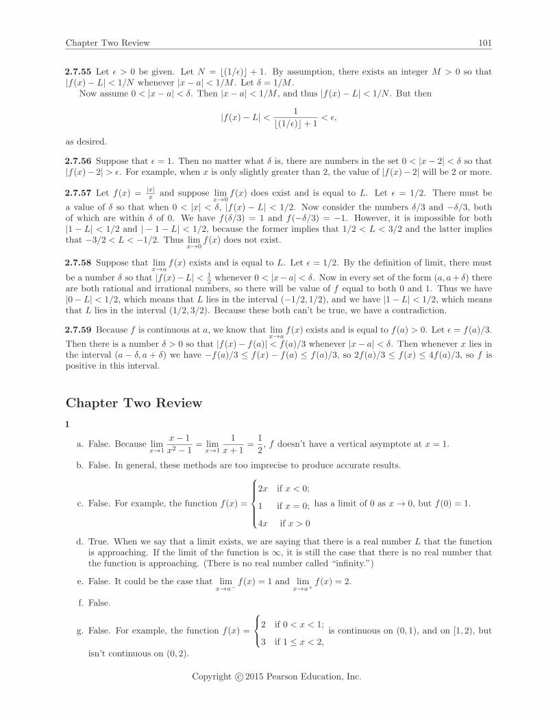
Chapter Two Review 101
2.7.55 Let ε > 0 be given. Let N = �(1/ε) + 1. By assumption, there exists an integer M > 0 so that|f(x)− L| < 1/N whenever |x− a| < 1/M . Let δ = 1/M .
Now assume 0 < |x− a| < δ. Then |x− a| < 1/M , and thus |f(x)− L| < 1/N . But then
|f(x)− L| < 1
�(1/ε) + 1< ε,
as desired.
2.7.56 Suppose that ε = 1. Then no matter what δ is, there are numbers in the set 0 < |x− 2| < δ so that|f(x)− 2| > ε. For example, when x is only slightly greater than 2, the value of |f(x)− 2| will be 2 or more.
2.7.57 Let f(x) = |x|x and suppose lim
x→0f(x) does exist and is equal to L. Let ε = 1/2. There must be
a value of δ so that when 0 < |x| < δ, |f(x) − L| < 1/2. Now consider the numbers δ/3 and −δ/3, bothof which are within δ of 0. We have f(δ/3) = 1 and f(−δ/3) = −1. However, it is impossible for both|1 − L| < 1/2 and | − 1 − L| < 1/2, because the former implies that 1/2 < L < 3/2 and the latter impliesthat −3/2 < L < −1/2. Thus lim
x→0f(x) does not exist.
2.7.58 Suppose that limx→a
f(x) exists and is equal to L. Let ε = 1/2. By the definition of limit, there must
be a number δ so that |f(x)−L| < 12 whenever 0 < |x− a| < δ. Now in every set of the form (a, a+ δ) there
are both rational and irrational numbers, so there will be value of f equal to both 0 and 1. Thus we have|0− L| < 1/2, which means that L lies in the interval (−1/2, 1/2), and we have |1− L| < 1/2, which meansthat L lies in the interval (1/2, 3/2). Because these both can’t be true, we have a contradiction.
2.7.59 Because f is continuous at a, we know that limx→a
f(x) exists and is equal to f(a) > 0. Let ε = f(a)/3.
Then there is a number δ > 0 so that |f(x)− f(a)| < f(a)/3 whenever |x− a| < δ. Then whenever x lies inthe interval (a − δ, a + δ) we have −f(a)/3 ≤ f(x) − f(a) ≤ f(a)/3, so 2f(a)/3 ≤ f(x) ≤ 4f(a)/3, so f ispositive in this interval.
Chapter Two Review
1
a. False. Because limx→1
x− 1
x2 − 1= lim
x→1
1
x+ 1=
1
2, f doesn’t have a vertical asymptote at x = 1.
b. False. In general, these methods are too imprecise to produce accurate results.
c. False. For example, the function f(x) =
⎧⎪⎪⎪⎨⎪⎪⎪⎩2x if x < 0;
1 if x = 0;
4x if x > 0
has a limit of 0 as x → 0, but f(0) = 1.
d. True. When we say that a limit exists, we are saying that there is a real number L that the functionis approaching. If the limit of the function is ∞, it is still the case that there is no real number thatthe function is approaching. (There is no real number called “infinity.”)
e. False. It could be the case that limx→a−
f(x) = 1 and limx→a+
f(x) = 2.
f. False.
g. False. For example, the function f(x) =
⎧⎨⎩2 if 0 < x < 1;
3 if 1 ≤ x < 2,is continuous on (0, 1), and on [1, 2), but
isn’t continuous on (0, 2).
Copyright c© 2015 Pearson Education, Inc.

102 Chapter 2. Limits
h. True. limx→a
f(x) = f(a) if and only if f is continuous at a.
2
a. f(−1) = 1 b. limx→−1−
f(x) = 3. c. limx→−1+
f(x) = 1.
d. limx→−1
f(x) does not exist. e. f(1) = 5. f. limx→1
f(x) = 5.
g. limx→2
f(x) = 4. h. limx→3−
f(x) = 3. i. limx→3+
f(x) = 5.
j. limx→3
f(x) does not exist.
3 This function is discontinuous at x = −1, at x = 1, and at x = 3. At x = −1 it is discontinuous becauselim
x→−1f(x) does not exist. At x = 1, it is discontinuous because lim
x→1f(x) = f(1). At x = 3, it is discontinuous
because f(3) does not exist, and because limx→3
f(x) does not exist.
4
a. The graph drawn by most graphing calculators andcomputer algebra systems doesn’t show the disconti-nuities where sin θ = 0.
b. It appears to be equal to 2
c. Using a trigonometric identity, limθ→0
sin 2θ
sin θ=
limθ→0
2 sin θ cos θ
sin θ. This can then be seen to be
limθ→0
2 cos θ = 2.
�6 �4 �2 2 4 6x
�2
�1
1
2y
True graph, showing discontinuitieswhere sin θ = 0.
�6 �4 �2 2 4 6x
�2
�1
1
2y
Graph shown without discontinuities.
5
a.x .9π/4 .99π/4 .999π/4 .9999π/4
f(x) 1.4098 1.4142 1.4142 1.4142
x 1.1π/4 1.01π/4 1.001π/4 1.0001π/4
f(x) 1.4098 1.4142 1.4142 1.4142
The limit appears to be approximately 1.4142.
b. limx→π/4
cos 2x
cosx− sinx= lim
x→π/4
cos2 x− sin2 x
cosx− sinx= lim
x→π/4(cosx+ sinx) =
√2.
Copyright c© 2015 Pearson Education, Inc.
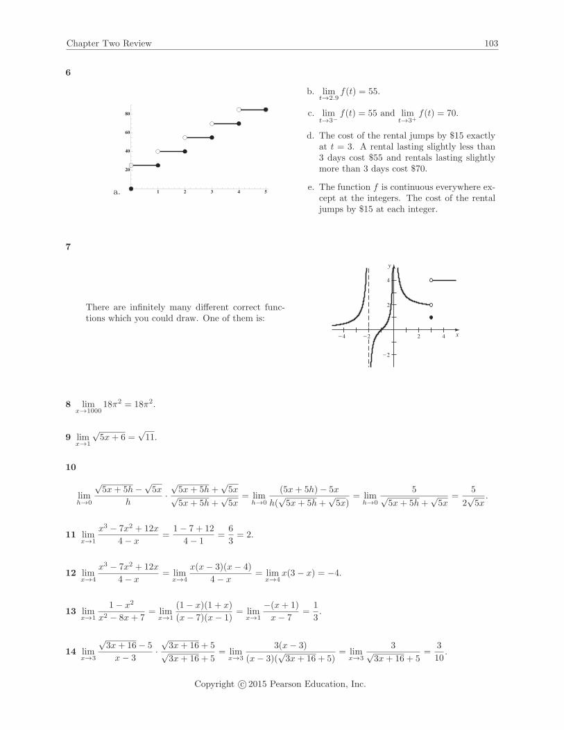
Chapter Two Review 103
6
a. 1 2 3 4 5
20
40
60
80
b. limt→2.9
f(t) = 55.
c. limt→3−
f(t) = 55 and limt→3+
f(t) = 70.
d. The cost of the rental jumps by $15 exactlyat t = 3. A rental lasting slightly less than3 days cost $55 and rentals lasting slightlymore than 3 days cost $70.
e. The function f is continuous everywhere ex-cept at the integers. The cost of the rentaljumps by $15 at each integer.
7
There are infinitely many different correct func-tions which you could draw. One of them is:
2
4
�2
2 4�2�4
y
x
8 limx→1000
18π2 = 18π2.
9 limx→1
√5x+ 6 =
√11.
10
limh→0
√5x+ 5h−√
5x
h·√5x+ 5h+
√5x√
5x+ 5h+√5x
= limh→0
(5x+ 5h)− 5x
h(√5x+ 5h+
√5x)
= limh→0
5√5x+ 5h+
√5x
=5
2√5x
.
11 limx→1
x3 − 7x2 + 12x
4− x=
1− 7 + 12
4− 1=
6
3= 2.
12 limx→4
x3 − 7x2 + 12x
4− x= lim
x→4
x(x− 3)(x− 4)
4− x= lim
x→4x(3− x) = −4.
13 limx→1
1− x2
x2 − 8x+ 7= lim
x→1
(1− x)(1 + x)
(x− 7)(x− 1)= lim
x→1
−(x+ 1)
x− 7=
1
3.
14 limx→3
√3x+ 16− 5
x− 3·√3x+ 16 + 5√3x+ 16 + 5
= limx→3
3(x− 3)
(x− 3)(√3x+ 16 + 5)
= limx→3
3√3x+ 16 + 5
=3
10.
Copyright c© 2015 Pearson Education, Inc.

104 Chapter 2. Limits
15
limx→3
1
x− 3
(1√x+ 1
− 1
2
)= lim
x→3
2−√x+ 1
2(x− 3)√x+ 1
· (2 +√x+ 1)
(2 +√x+ 1)
= limx→3
4− (x+ 1)
2(x− 3)(√x+ 1)(2 +
√x+ 1)
= limx→3
−(x− 3)
2(x− 3)(√x+ 1)(2 +
√x+ 1)
= limx→3
− 1
2√x+ 1(2 +
√x+ 1)
= − 1
16.
16 limt→1/3
t− 13
(3t− 1)2= lim
t→1/3
3t− 1
3(3t− 1)2= lim
t→1/3
1
3(3t− 1), which does not exist.
17 limx→3
x4 − 81
x− 3= lim
x→3
(x− 3)(x+ 3)(x2 + 9)
x− 3= lim
x→3(x+ 3)(x2 + 9) = 108.
18 Note that p5−1p−1 = p4 + p3 + p2 + p+ 1. (Use long division.)
limp→1
p5 − 1
p− 1= lim
p→1(p4 + p3 + p2 + p+ 1) = 5.
19 limx→81
4√x− 3
x− 81= lim
x→81
4√x− 3
(√x+ 9)( 4
√x+ 3)( 4
√x− 3)
= limx→81
1
(√x+ 9)( 4
√x+ 3)
=1
108.
20 limθ→π/4
sin2 θ − cos2 θ
sin θ − cos θ= lim
θ→π/4
(sin θ − cos θ)(sin θ + cos θ)
sin θ − cos θ= lim
θ→π/4(sin θ + cos θ) =
√2.
21 limx→π/2
1√sin x
− 1
x+ π/2=
0
π= 0.
22 The domain of f(x) =√
x−1x−3 is (−∞, 1] and (3,∞), so lim
x→1+f(x) doesn’t exist.
However, we have limx→1−
f(x) = 0.
23
a. �1.0 �0.5 0.5 1.0x
0.8
1.0
1.2
1.4
y
b. Because limx→0
cosx = limx→0
1
cosx= 1, the squeeze
theorem assures us that limx→0
sinx
x= 1 as well.
24 Note that limx→0
(sin2 x + 1) = 1. Thus if 1 ≤ g(x) ≤ sin2 x + 1, the squeeze theorem assures us that
limx→0
g(x) = 1 as well.
25 limx→5
x− 7
x(x− 5)2= −∞.
26 limx→−5+
x− 5
x+ 5= −∞.
Copyright c© 2015 Pearson Education, Inc.

Chapter Two Review 105
27 limx→3−
x− 4
x2 − 3x= lim
x→3−
x− 4
x(x− 3)= ∞.
28 limx→0+
u− 1
sinu= −∞.
29 limx→0−
2
tanx= −∞.
30
First note that f(x) = x2−5x+6x2−2x = (x−3)(x−2)
x(x−2) .
a. limx→0−
f(x) = limx→0−
(x− 3)(x− 2)
x(x− 2)= ∞.
limx→0+
f(x) = limx→0+
(x− 3)(x− 2)
x(x− 2)= −∞.
limx→2−
f(x) = limx→2−
x− 3
x= −1
2.
limx→2+
f(x) = limx→2+
x− 3
x= −1
2.
b. By the above calculations and the definition ofvertical asymptote, f has a vertical asymptote atx = 0.
c. Note that the actual graph has a “hole” at thepoint (2,−1/2), because x = 2 isn’t in the domain,but lim
x→2f(x) = −1/2.
�4 �2 2 4x
�5
5
y
31 limx→∞
2x− 3
4x+ 10= lim
x→∞2− (3/x)
4 + (10/x)=
2
4=
1
2.
32 limx→∞
x4 − 1
x5 + 2= lim
x→∞(1/x)− (1/x5)
1 + (2/x5)=
0− 0
1 + 0= 0.
33 limx→−∞(−3x3 + 5) = ∞.
34 limx→∞
x√4x2 + 1
= limx→∞
1√4 + 1/x2
=1
2.
35 limx→∞
√25x2 + 8
x+ 2= lim
x→∞
√25 + 8/x2
1 + 2/x= 5.
36 Because cos r oscillates between −1 and 1, this limit does not exist. For any N > 0, there are values of r
with |r| > N such that cos r = 0, cos r = 1, or cos r = −1. Thus the value of the expression1
cos r + 1takes
on the values 1, 1/2, and is undefined infinitely often as r → ∞.
37 limx→∞
4x3 + 1
1− x3= lim
x→∞4 + (1/x3)
(1/x3)− 1=
4 + 0
0− 1= −4. A similar result holds as x → −∞. Thus, y = −4 is a
horizontal asymptote as x → ∞ and as x → −∞.
38 First note that√
1x2 =
∣∣ 1x
∣∣ =⎧⎨⎩
1x if x > 0;
− 1x if x < 0.
.
limx→∞
x+ 1√9x2 + x
= limx→∞
1 + (1/x)√9 + 1
x
=1
3.
Copyright c© 2015 Pearson Education, Inc.

106 Chapter 2. Limits
On the other hand, limx→−∞
x+ 1√9x2 + x
= limx→∞
1 + (1/x)
−√
9 + 1x
= −1
3.
So y = 13 is a horizontal asymptote as x → ∞, and y = − 1
3 is a horizontal asymptote as x → −∞.
39 limx→±∞
12x2
√16x4 + 7
= limx→±∞
12√16 + 7/x4
= 3.
40 limx→±∞
3
√8x+ 1
x− 3= lim
x→±∞3
√8 + 1/x
1− 3/x=
3√8 = 2.
41 limx→±∞
x2 − x
x2 − 1= lim
x→±∞x
x+ 1= lim
x→±∞1
1 + 1/x= 1, so that f(x) has a horizontal asymptote of y = 1.
There is a vertical asymptote where x+ 1 = 0, i.e. for x = −1.
42 Note that f(x) = 2x2+62x2+3x−2 = 2(x2+3)
(2x−1)(x+2) .
We have limx→∞ f(x) = lim
x→∞2 + 6/x2
2 + 3/x− 2/x2= 1. A similar result holds as x → −∞.
limx→1/2−
f(x) = −∞. limx→1/2+
f(x) = ∞.
limx→−2−
f(x) = ∞. limx→−2+
f(x) = −∞.
Thus, y = 1 is a horizontal asymptote as x → ∞ and as x → −∞. Also, x = 12 and x = −2 are vertical
asymptotes.
43 limx→∞
3x2 + 2x− 1
4x+ 1= lim
x→∞3x2 + 2x− 1
4x+ 1· 1/x1/x
= limx→∞
3x+ 2− 1/x
4 + 1/x= ∞.
limx→−∞
3x2 + 2x− 1
4x+ 1= lim
x→−∞3x2 + 2x− 1
4x+ 1· 1/x1/x
= limx→−∞
3x+ 2− 1/x
4 + 1/x= −∞.
By long division, we can write f(x) as f(x) = 3x4 + 5
16 + −21/164x+1 , so the line y = 3x
4 + 516 is the slant
asymptote.
44 limx→∞
9x2 + 4
(2x− 1)2= lim
x→∞9x2 + 4
4x2 − 4x+ 1· 1/x
2
1/x2= lim
x→∞9 + 4/x2
4− 4/x+ 1/x2=
9
4.
limx→−∞
9x2 + 4
(2x− 1)2= lim
x→−∞9x2 + 4
4x2 − 4x+ 1·1/x
2
1/x2= lim
x→−∞9 + 4/x2
4− 4/x+ 1/x2=
9
4. Because there is a horizontal
asymptote, there is not a slant asymptote.
45 limx→∞
1 + x− 2x2 − x3
x2 + 1= lim
x→∞1 + x− 2x2 − x3
x2 + 1· 1/x
2
1/x2= lim
x→∞1/x2 + 1/x− 2− x
1 + 1/x2= −∞.
limx→−∞
1 + x− 2x2 − x3
x2 + 1= lim
x→−∞1 + x− 2x2 − x3
x2 + 1· 1/x
2
1/x2= lim
x→−∞1/x2 + 1/x− 2− x
1 + 1/x2= ∞.
By long division, we can write f(x) as f(x) = −x−2+ 2x+3x2+1 , so the line y = −x−2 is the slant asymptote.
46 limx→∞
x(x+ 2)3
3x2 − 4x= lim
x→∞x4 + 6x3 + 12x2 + 8x
3x2 − 4x· 1/x
2
1/x2= lim
x→∞x2 + 6x+ 12 + 8/x
3− 4/x= ∞.
limx→−∞
x(x+ 2)3
3x2 − 4x= lim
x→−∞x4 + 6x3 + 12x2 + 8x
3x2 − 4x· 1/x
2
1/x2= lim
x→−∞x2 + 6x+ 12 + 8/x
3− 4/x= ∞.
Because the degree of the numerator of this rational function is two more than the degree of the denom-inator, there is no slant asymptote.
47 f is discontinuous at 5, because f(5) does not exist, and also because limx→5
f(x) does not exist
48 g is discontinuous at 4 because limx→4
g(x) = limx→4
(x+ 4)(x− 4)
x− 4= 8 = g(4).
Copyright c© 2015 Pearson Education, Inc.

Chapter Two Review 107
49 h is not continuous at 3 because limx→3−
h(x) does not exist, so limx→3
h(x) does not exist.
50 g is continuous at 4 because limx→4
g(x) = limx→4
(x+ 4)(x− 4)
x− 4= 8 = g(4).
51 The domain of f is (−∞,−√5] and [
√5,∞), and f is continuous on that domain.
52 The domain of g is all x such that x2 − 5x+6 = (x− 3)(x− 2) ≥ 0, i.e. (−∞, 2]∪ [3,∞). g is continuouson its domain. At x = 2 the function is continuous from the left only; at x = 3 it is continuous from theright only.
53 The domain of h is (−∞,−5), (−5, 0), (0, 5), (5,∞), and like all rational functions, it is continuous onits domain.
54 The domain of g is the set of real numbers x such that x ≥ 0 (so that√x is defined). g is continuous on
its domain; at x = 0 it is continuous from the right only.
55 In order for g to be left continuous at 1, it is necessary that limx→1−
g(x) = g(1), which means that
a = 3. In order for g to be right continuous at 1, it is necessary that limx→1+
g(x) = g(1), which means that
a+ b = 3 + b = 3, so b = 0.
56
a. Because the domain of h is (−∞,−3] and [3,∞), there is no way that h can be left continuous at 3.
b. h is right continuous at 3, because limx→3+
h(x) = 0 = h(3).
57
One such possible graph is pictured to the right.
0.5 1.0 1.5 2.0x
1.5
2.0
2.5
3.0
3.5
4.0y
58 a. Consider the function f(x) = x5 + 7x+ 5. f is continuous everywhere, and f(−1) = −3 < 0 whilef(0) = 5 > 0. Therefore, 0 is an intermediate value between f(−1) and f(0). By the IVT, there musta number c between 0 and 1 so that f(c) = 0.
b. Using a computer algebra system, one can find that c ≈ −0.691671 is a root.
59
a. Any such rectangle with length x has width y = 100/x, so its perimeter is
P (x) = 2x+ 2y = 2x+200
x.
b. P is continuous for x > 0. P (10) = 40 while P (30) = 60 + 20030 > 60. Thus by the Intermediate Value
Theorem, there must be some x with 10 ≤ x ≤ 30 and P (x) = 50.
Copyright c© 2015 Pearson Education, Inc.
108 Chapter 2. Limits
c. The rectangle with perimeter 50 can be determined by solving P (x) = 50.
2x+200
x= 50
2x2 − 50x+ 200 = 0
x = 5, 20
So a perimeter of 50 occurs for a 5× 20 or a 20× 5 rectangle.
d. If there were a rectangle with perimeter 30, it would be a solution to P (x) = 30, so
2x+200
x= 30, 2x2 − 30x+ 200 = 0
The discriminant of this quadratic is 900− 1600 < 0, so the quadratic has no (real) solution.
e. Plotting P (x) for various viewing windows seems to show that the smallest possible perimeter is 40,for a 10× 10 rectangle.
60 Let ε > 0 be given. Let δ = ε/5. Now suppose that 0 < |x− 1| < δ.Then
|f(x)− L| = |(5x− 2)− 3| = |5x− 5|= 5|x− 1| < 5 · ε
5= ε.
61 Let ε > 0 be given. Let δ = ε. Now suppose that 0 < |x− 5| < δ.Then
|f(x)− L| =∣∣∣∣x2 − 25
x− 5− 10
∣∣∣∣ =∣∣∣∣ (x− 5)(x+ 5)
x− 5− 10
∣∣∣∣ = |x+ 5− 10|
= |x− 5| < ε.
62
a. Assume L > 0. (If L = 0, the result follows immediately because that would imply that the functionf is the constant function 0, and then f(x)g(x) is also the constant function 0.) Assume that δ1 is anumber so that |f(x)| ≤ L for |x− a| < δ1.
Let ε > 0 be given. Because limx→a
g(x) = 0, we know that there exists a number δ2 > 0 so that
|g(x)| < ε/L whenever 0 < |x− a| < δ2. Let δ = min(δ1, δ2).
Then|f(x)g(x)− 0| = |f(x)||g(x)| < L · ε
L= ε,
whenever 0 < |x− a| < δ.
b. Let f(x) = x2
x−2 . Then
limx→2
f(x)(x− 2) = limx→2
x2(x− 2)
x− 2= lim
x→2x2 = 4 = 0.
This doesn’t violate the previous result because the given function f is not bounded near x = 2.
c. Because |H(x)| ≤ 1 for all x, the result follows directly from part a) of this problem (using L = 1,a = 0, f(x) = H(x), and g(x) = x).
63 Let N > 0 be given. Let δ = 1/ 4√N . Suppose that 0 < |x− 2| < δ. Then |x− 2| < 1
4√N, so 1
|x−2| >4√N ,
and 1(x−2)4 > N , as desired.
Copyright c© 2015 Pearson Education, Inc.