maintenance and investment: complements or substitutes… · maintenance and investment:...
TRANSCRIPT
Maintenance and Investment: Complements orSubstitutes? A Reappraisal
R. Boucekkine∗, G. Fabbri†, F. Gozzi‡
April 28, 2009
Abstract
A benchmark AK optimal growth model with maintenance expendituresand endogenous utilization of capital is considered within an explicit vin-tage capital framework. Scrapping is endogenous, and the model allowsfor a clean distinction between age and usage dependent capital deprecia-tion and obsolescence. It is also shown that in this set-up past investmentprofile completely determines the size of current maintenance expendi-tures. Among other findings, a closed-form solution to optimal dynam-ics is provided taking advantage of very recent development in optimalcontrol of infinite dimensional systems. More importantly, and in con-trast to the pre-existing literature, we study investment and maintenanceco-movements without any postulated ad-hoc depreciation function. Inparticular, we find that optimal investment and maintenance do move to-gether in the short-run in response to neutral technological shocks, whichseems to be more consistent with the data.
Keywords: Maintenance, investment, optimal control, dynamic program-ming, infinite dimensional problem
JEL classification: E22, E32, O40
∗Corresponding author. Department of Economics and CORE, Place Montesquieu 3,Universite catholique de Louvain, Louvain-La-Neuve, Belgium; Department of Economics,University of Glasgow, Scotland. E-mail: [email protected]
†Dipartimento di Studi Economici, Universita di Napoli ”‘Parthenope”’, Naples, Italy.E-mail: [email protected]
‡Dipartimento di Scienze Economiche ed Aziendali, Universita LUISS - Guido Carli Rome,Italy. E-mail: [email protected]
1
1 Introduction
There is an increasing effort to incorporate maintenance and repair activitiesin the core of investment theory, and therefore in the core of growth theory.While traditional Jorgensonian investment theory relies on the assumption ofconstant capital depreciation rate, several authors have been pointing at thenumerous shortcomings arising from such an assumption, therefore challengingthe ability of the standard model to account for the investment decision eitherat the firm or the aggregate levels. Feldstein and Rothschild (1974) and Nickell(1975) are two pioneering works in this respect.
Yet the incorporation of maintenance and repair costs in macroeconomicmodels of investment and growth has truly started with the illuminating workof McGrattan and Schmitz (1999). Indeed the lack of economy-wide surveysassessing the importance of maintenance costs was usually invoked to disregardthem. McGrattan and Schmitz were the first to exploit a Canadian (economy-wide) survey, and to highlight why and how investment theory can account forthese costs. Their argument was actually easy to make as maintenance andrepair expenditures averaged about 6% of the Canadian GDP and nearly 50%of spending on new equipment over the period 1961-1993.
Since then, several research projects have been launched on the topic. Letus mention briefly some of the directions taken. A first bulk of papers studiedthe implications of accounting for maintenance expenditures within otherwisestandard models of investment and/or growth. For example Licandro et al.(2001) introduced maintenance in optimal growth by specifying capital de-preciation as a decreasing function of maintenance. They studied accordinglyhow the latter affects the typical convergence properties inherent to neoclas-sical theory. Boucekkine and Ruiz-Tamarit (2003) took a tighter avenue, thestandard neoclassical investment firm model,1 but they allowed for a moreflexible relationship between depreciation, maintenance expenditures and therate of capital utilization. They showed that depending on some deep charac-teristics of the latter relationship, investment and maintenance decisions canrespond (or not) in the same way to various neutral technological shocks. Co-movements of investment and maintenance are the central motivation of ourpaper, so we will come back later to this point. Note however that the previouspapers only provide characterizations around steady state equilibria, while ourpaper solves out the short-term optimal dynamics.
On the quantitative macroeconomics ground, more papers have been writ-ten recently.2 Important contributions to this line of research are due toKalaitzidakis and Kalyvitis (2004, 2005) who studied how maintenance of pub-lic capital affects long-term growth and how to fix optimally maintenance ex-penditures in this respect. More recently, Boucekkine et al. (2008, 2009) have
1Another paper taking this avenue is Kalyvitis (2006) who empirically found that the in-corporation of maintenance and repair expenditures into the q-model of investment improvesthe relevance of the latter.
2An early investigation of the role of maintenance in the business cycle is due to Collardand Kollintzas (2000).
2
shown how to incorporate maintenance and support costs in vintage capitalmodels.3 In contrast to all the other papers listed so far, the approach fol-lowed does not build on a given functional form directly relating maintenanceto depreciation (initiated by McGrattan and Schmitz, 1999) but derives de-preciation partly as a result of the endogenous scrapping decision of obsoletecapital items. Therefore the main advantage of the approach is to allow foran endogenous identification of depreciation due to obsolescence on one hand,and depreciation due to aging and utilization on the other. Boucekkine et al.(2009) consider a multi-sector model with both investment-specific and neu-tral technological progress, and Cobb-Douglas production function in the finalgoods sector. In contrast, the model developed in the 2008 paper is a muchsimpler AK one-sector model with neutral technological progress.
Our paper also takes this approach. In particular, the baseline modelconsidered is a version of the AK model described by Boucekkine et al. (2008).However, while these authors focus on the steady state, we are able to:
1. find a closed-form solution to optimal dynamics by applying the dynamicprogramming strategy developed by Fabbri and Gozzi (2008a);
2. and accordingly to study how optimal investment and maintenance movein response to technological shocks, not only in the long-run, but also inthe short-run.
In this sense, our paper has a double technical contribution: on one hand,it derives a closed-form solution to the optimal dynamics in the vintage AKmodel of Boucekkine et al. (2008), and on the other, it shows how to apply thedynamic programming approach of Fabbri and Gozzi to an AK model withendogenous scrapping. The first application, provided by the authors them-selves, was on the AK vintage capital model of Boucekkine et al. (2005) whichhas exogenous scrapping time. Because the involved optimal control problemhas a differential-difference state equation, the problem is infinite dimensional,and the dynamics cannot be studied with the standard techniques. Technicaldetails will be given along the way.
More importantly, our paper brings out an original contribution to an im-portant question in the literature, investment and maintenance co-movements.In the earlier papers devoted to this issue, notably those devoted to the studyof business fluctuations (see Collard and Kollintzas (2000) and specially Li-candro and Puch (2000)), the specification of the depreciation function waschosen in order to replicate some key stylized facts. To make our argumentneater and more precise, whence the depreciation function δ(U,M) is postu-lated, with U the capital utilization rate and M maintenance expenditures,assumptions on second-order derivatives of function δ(U,M) are made to fitthe data. In particular, it turned out that the sign of the second-order crossderivative δUM (U,M) is crucial for the shape of investment and maintenanceco-movements. As mentioned above, Boucekkine and Ruiz-Tamarit (2003)have provided with a systematic analysis of the problem depending on the
3Another paper taking this approach is due to Saglam and Veliov (2008).
3
sign of this cross-derivative. When δUM (U,M) ≥ 0, then investment andmaintenance move in the same direction (Proposition 3, Boucekkine and Ruiz-Tamarit, 2003). This case is considered to be compatible with data by Li-candro and Puch (2000). However, when δUM (U,M) < 0, things are muchtrickier, and under certain circumstances, maintenance can act as a substituteto investment, as previously claimed by McGrattan and Schmitz (1999). Ourpaper offers a sounder framework to study these co-movements. First of all,in contrast to Boucekkine and Ruiz-Tamarit (2003), we leave the steady stateand address the problem along optimal transitional dynamics. Second of all,in contrast to the papers mentioned just above, there is no postulated depre-ciation function, and the depreciation rate is identified in particular throughan endogenous scrapping decision. Our main result is that in such a frame-work, optimal investment and maintenance do move together in the short-runin response to neutral technological shocks.
The paper is organized as follows. Section 2 gives a brief description of theAK model of Boucekkine et al. (2008) (from now BRM model). Section 3 istwofold: it first presents the infinite dimensional optimal control problem underconsideration recalling the principles of the dynamic programming approachused to solve it, then (from Subsection 3.2 on) it attacks the problem derivingclosed form solutions and studying the properties of the optimal paths. Section4 compiles some numerical exercises conducted to study optimal investmentand maintenance co-movements. Section 5 concludes.
2 The model
The model is one-sector AK model with vintage capital. The aggregate pro-duction function is AK:
Y (t) = Akt, A > 0where kt is the stock of capital at time t, which is given by
kt =∫ t
t−T (t)x (z, t) i (z) dz (1)
where i (z) is investment at time z, and T (t) is the age of the oldest machinestill in use at time t. x (z, t) is a key decision variable in the model: The morecapital goods of vintage z are efficient at time t, the more they are used andthe larger is x(z, t). The latter thus measures at the same time the utilizationintensity and productivity of machines of vintage z at time t. Notice howeverthat strictly speaking, there is no investment-specific technical progress in ourmodel, the unique (exogenous) technical progress indicator in the model is pa-rameter A, which may reflect the state of disembodied (neutral) technologicalchange in the sense that all operating machines are affected in the same wayby technological accelerations through A. By taking this avenue, comparisonwith more standard RBC approaches like Licandro and Puch (2000) is moreappropriate.
Another interesting specification in BRM is the introduction of mainte-nance and repair expenditures. It extends a previous specification of Whelan
4
(2002) by assuming a variable maintenance cost.4 More specifically, the unitmaintenance and repair cost of vintage z at time t is assumed to be an increas-ing function of its age, t− z, and its relative average productivity,
ω (t− z, x (z, t)) = βeγ(t−z)x (z, t)µ + η, β > 0 , η > 0, µ > 1.
When β = 0, we get Whelan’s specification, maintenance costs becomeequal to a constant support cost. Notice that the specification is completelygeneric: beside aging, maintenance costs increase with utilization. µ > 1and η > 0 are needed to have a finite optimal choice of utilization and for afinite time scrapping to be possible respectively. Indeed, production net of themaintenance and repair costs is
y (t) =∫ t
t−T (t)B (t− z, x (z, t)) i (z) dz, (2)
whereB (t− z, x (z, t)) = Ax (z, t)− ω (t− z, x (z, t)) (3)
is the average (and marginal) profitability of vintage z at time t. The uti-lization intensities x(z, t) are chosen to maximize the average profitability,B (t− z, x (z, t)). The first order condition of this maximization problem im-plies that x(z, t) depends only on the difference t− z and
x (t− z) = x0e− γ
µ−1(t−z)
. (4)
where x0 =(
Aβµ
) 1µ−1 , inducing a decreasing age profile for utilization. The
profile is shifted upward by neutral technological improvements through pa-rameter A, and shifted down if the maintenance technology worsens throughparameters β and γ.
Finally a machine of vintage z is scrapped whence its profitability drops tozero. Substitution from x (t− z) into (3) yields:
B (t− z) ≡ B (t− z, x (t− z)) = Ωe− γ
µ−1(t−z) − η, (5)
where Ω = (µ − 1) β xµ0 , which implies that a vintage will be utilized until a
finite age T > 0 such that
B (T ) = Ωe− γ
µ−1T − η = 0. (6)
It is easy to prove that whence Ω > η > 0, a finite (and positive) scrappingtime exists (and is unique: T = µ−1
γ ln Ωη ). It is also straightforward to see that
T is an increasing function of A and a decreasing function of β, γ and η. Tech-nological improvement through A increases the profitability of ALL vintages,leading to lengthening their lifetime. Notice that this property arises becausetechnological progress is neutral in the latter case. Investment-specific techno-logical progress would lead to shorter lifetimes, see Boucekkine et al. (2009).Here, since we are interested in investment and maintenance co-movements,and mainly for comparison with the results gathered by Licandro and Puch
4Whelan (2002) considered a constant support cost for any vintage at any time.
5
(2000) or Boucekkine and Ruiz-Tamarit (2003) for example, we consider neu-tral technological progress accelerations in a one-sector model.5
Finally and as announced in the introduction, our model allows to dis-entangle obsolescence and physical depreciation in a quite easy and naturalway. The stock of capital at time t can vary due to (i) gross investment, (ii)the change of the relative average productivity of capital, which is physicaldepreciation, and (iii) the scrapping of unprofitable vintages, which is calledobsolescence. Differentiating equation (1), and using that x (t− z) is given by(4), yields the following evolution law of capital:
·k (t) = x0i (t)− (ξ (t) + δ) k (t) (7)
whereξ (t) = x0e
− γµ−1
T i(t− T )k(t)
(8)
is related to the fraction of scrapped capital at time t, and
δ =γ
µ− 1(9)
is the decline rate of the average relative productivity or equivalently utilizationintensity of each vintage. For quite intuitive reasons, we shall call ξ(t) the rateof obsolescence, and the constant δ the rate of physical depreciation since it isrelated to aging and usage.
There is a big difference between the behavior of the obsolescence rate andthe physical depreciation rate. While the physical depreciation rate is constant,the obsolescence rate is not so because it depends on the scrapped investment-capital ratio and it could fluctuate due to the existence of echo effects thatgenerally characterize the dynamics of vintage capital models as proved byBoucekkine et al. (2005). On the other hand, and more importantly for ourpaper, the rate of physical depreciation need not respond in the same way totechnological accelerations or other shocks. For example, if A increases, therate δ is unaffected while the obsolescence rate ξ(t) is likely to respond giventhat the impact of A’s increase on lifetime T does affect ξ(t) in several ways.We shall come back to these questions later.
In the next section, after presenting the optimal control problem tackledby BRM, we provide with the dynamic programming strategy allowing to findout a closed-form solution to the optimal dynamics.
3 The optimal control problem
The optimal growth problem stated in BRM is standard in that it consistsin maximizing intertemporal utility subject to the AK production technology.The per-period utility function is CARA (with 1
σ , σ > 0, the elasticity of in-tertemporal substitution in consumption), and an interesting feature in BRM’s
5Needless to say, considering investment-specific technological progress requires at leasttwo sectors, consumption and capital sectors. See Boucekkine et al. (2009).
6
approach is the possibility to save one control variable, maintenance, by usingthe net production function (2). Needless to say, capital, maintenance andreplacement investment can be reconstructed from the computed controls andstates. Indeed, these three variables, k(·), M(t) and ir(·) respectively, aredetermined by:
k(t) =∫ t
t−Tx0e
−δ(t−τ)i(τ)dτ, (10)
M(t) =∫ t
t−Tω(t− τ, x(τ, t)i(τ)dτ =
∫ t
t−T
[eγ(t−τ)xµ
0e−δµ(t−τ) + η]i(τ)dτ
(11)=
∫ t
t−T
[Ω
µ− 1e−δ(t−τ) + η
]i(τ)dτ
and
ir(t) = δk(t) + x0e−δT i(t− T ) = x0
[∫ t
t−Tδe−δ(t−τ)i(τ)dτ + e−δT i(t− T )
].
(12)
It should be also noted that by the same argument, we can also identify theoptimal path of the endogenous obsolescence rate, ξ(t), thanks to equation (8).We will be then able to investigate, among others, the issue of substitutabilityVs complementarity of investment and maintenance expenditures. Because ofthe delayed integral representation of capital, maintenance and replacementinvestment in terms of the investment profile, see (10)-(12), the co-movementsof each of the three variables and gross investment are not obvious at all. Yet(10)-(12) exhibit a quite striking property, at least for maintenance: by (11),past investment profile i(z), t − T ≤ z ≤ t, completely determines the sizeof maintenance expenditures at t. This is not at all the way maintenance ex-penditures are determined in the recent literature following the path-breakingcontribution of McGrattan and Schmitz (1999). Therefore, our modeling doesbring a new approach to the study of the relationship between investment andmaintenance.
Let us now dig deeper in our optimal control problem. If consumption isc(t) = y(t)− i(t), then the optimal control problem is:
Max
∫ +∞
0
(y(t)− i(t)
1− σ
)1−σ
dt
subject to (for t ≥ 0):
y(t) =∫ t
t−T(Ωe−δ(t−s) − η)i(s) ds, i(s) given for s ∈ [−T, 0). (13)
The integral equation (13) is the net production function obtained using(2) and (5), T is the scrapping time identified by (6). It is possible to put theintegral equation above into a more standard differential equation by differen-tiating it. Then we get the following state equation (for t ≥ 0):
y(t) = (Ω− η)i(t)− δΩ∫ 0
−Teδri(r + t)dr, i(s) given for s ∈ [−T, 0). (14)
7
The problem has some standard features but it entails a definitely non-standard characteristic. It has one control, investment, and one state, netoutput. The state equation is a delay-differential equation, which implies thatthe problem is infinite dimensional. BRM only studied some properties ofthe balanced growth paths. This section is devoted to provide a closed-formsolution to optimal dynamics, including asymptotics. The technique used isinspired by Fabbri and Gozzi (2008a). We first explain its general principles,then we apply it to BRM.
Apart from small changes some results given in this section can be provedas in Fabbri and Gozzi (2008a) so we do not repeat them here simply referringto that paper. Nevertheless some other results (especially Propositions 3.2,3.3, 3.10, 3.11 and Theorems 3.2, 3.3) are essentially different and cannot bederived from known results since they use the peculiar characteristics of theBRM model. We prove them in the Appendix A.
3.1 The method
The optimal control problem is treated following the procedure used by Fab-bri and Gozzi (2008a).6 First we write the problem as an optimal controlproblem driven by a Delay Differential Equation (DDE) (Section 3.2) givingsome preliminary results. Then we translate it7 as an optimal control prob-lem driven by an Ordinary Differential Equation (ODE) (without delay) in asuitable Hilbert space. At that point we apply the dynamic programming tothis problem: we write and solve explicitly the HJB equation in the Hilbertspace, we prove that the solution is the value function and we use the explicitexpression of the value function to find the optimal feedback in closed form.
Solving the HJB equation is in general a difficult task: as well known, itis impossible in general to find an explicit solution even to finite dimensionalHJB equations, so, a fortiori, explicit solutions of infinite dimensional HJBequations are very rare. Here we have to use the particular structure of theproblem. The explicit form of the value function allows us to solve the infinitedimensional problem and to find the closed loop solutions. All the job requiredto handle the infinite dimensional nature of the problem is performed in Sub-section 3.3. Eventually we translate back the solution to the DDE setting andwe find a closed loop solution of our original problem (Subsection 3.4).
3.2 Statement of the optimal control problem in DDE formand preliminary results
We first introduce a notation useful to rewrite more formally (14):Notation 3.1 We call ι : [−T, 0) → R+, the initial datum, i : [0,+∞) → R+
the control strategy and ı : [−T, +∞) → R+ the function:6We briefly outline the procedure in this subsection and we refer the reader to Fabbri and
Gozzi (2008a) (Sections 1.2, 1.3, 2) and to its extended version Fabbri and Gozzi (2008b) formore details on the techniques and on the literature.
7Using the techniques introduced by Delfour (1986) and Vinter and Kwong (1981), seealso Bensoussan et al. (2007) chapter 4.
8
ı(s) =
ι(s) s ∈ [−T, 0)i(s) s ∈ [0, +∞). (15)
As explained before, standard pointwise initial conditions are not enough todetermine solution paths to the DDEs involved. Rather we need an initialfunction on a particular time span depending on the particular delays involved.Accordingly, we shall work on functional spaces. Hereafter, we give the neededconcepts to get through this problem, four useful functional spaces are defined.
L2([−T, 0);R) denotes to the space of all functions from [−T, 0) to R thatare Lebesgue measurable and square integrable. L2
loc([0, +∞);R) is the spaceof all functions from [0, +∞) to R that are Lebesgue measurable and squareintegrable on all bounded intervals. W 1,2([−T, 0);R) denotes the space ofthe functions in L2([−T, 0);R) whose first derivative belongs to L2([−T, 0);R)too. Eventually W 1,2
loc ([0, +∞);R) denotes the space of all functions be-longing, together their first derivatives, to L2
loc([0, +∞);R). We denote byL2([−T, 0);R+) the subset of L2([−T, 0);R) made by positive functions. Sim-ilarly we define L2
loc([0, +∞);R+).
The state equation (14) can now be written as the following DDE (on R+):
y(t) = (Ω− η)ı(t)− δΩ∫ 0−T eδr ı(r + t)dr
ı(s) = ι(s) ∀s ∈ [−T, 0)y(0) =
∫ 0−T ι(s)(Ωeδs − η)ds
(16)
where ι(·) and y(0) are the initial conditions.8 We will assume ι(·) ≥ 0 andι(·) 6≡ 0 so y(0) > 0. Moreover we impose that ι(·) ∈ L2([−T, 0),R+). Thanksto what we said in the previous sections T, Ω, δ, σ, ρ are strictly positive con-stants, moreover we assume that σ 6= 1. For every i : R+ → R locally integrableand every ι ∈ L2([−T, 0),R) the (16) admits a unique locally absolutely con-tinuous solution (so (16) must be understood in integral sense). Thanks to (6)the solution is:
yι,i(t) =∫ t
(t−T )ı(s)(Ωe−δ(t−s) − η)ds (17)
The functional to maximize is
J(ι; i)def=
∫ ∞
0e−ρs (yι,i(t)− i(t))1−σ
(1− σ)ds
over the set
Iιdef= i(·) ∈ L2
loc([0, +∞);R+) : i(t) ∈ [0, yι,i(t)] for almost all t ∈ R+.The choice of Iι ensures that yι,i(·) ∈ W 1,2
loc ([0, +∞);R+) and then it is contin-uous. We call Problem (P) the problem of finding an optimal control strategyi.e. an i∗(·) ∈ Iι such that:
J(ι; i∗) = V (ι)def= sup
i(·)∈Iι
∫ ∞
0e−ρs (yι,i(t)− i(t))1−σ
(1− σ)ds
. (18)
V is called value function.8Indeed y(0) is not a datum as it depends on ι(·) but (as we will see below) it is convenient
to consider it a datum.
9
3.2.1 Preliminary results
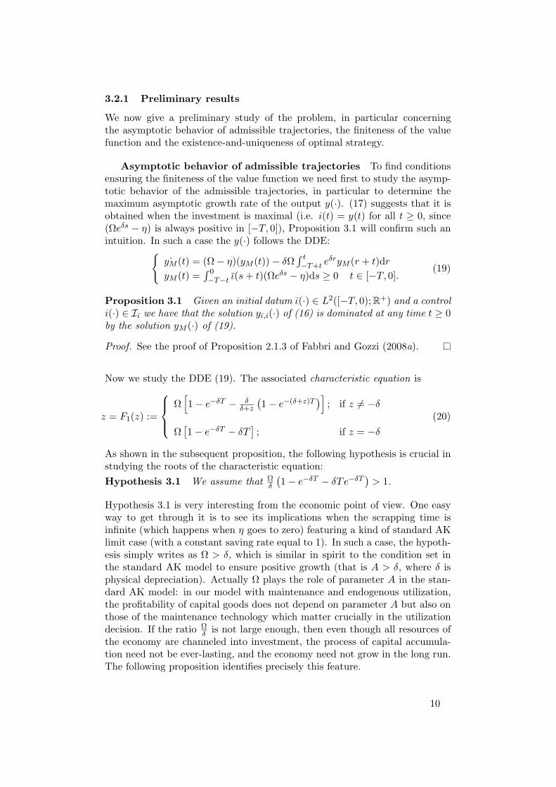
We now give a preliminary study of the problem, in particular concerningthe asymptotic behavior of admissible trajectories, the finiteness of the valuefunction and the existence-and-uniqueness of optimal strategy.
Asymptotic behavior of admissible trajectories To find conditionsensuring the finiteness of the value function we need first to study the asymp-totic behavior of the admissible trajectories, in particular to determine themaximum asymptotic growth rate of the output y(·). (17) suggests that it isobtained when the investment is maximal (i.e. i(t) = y(t) for all t ≥ 0, since(Ωeδs − η) is always positive in [−T, 0]), Proposition 3.1 will confirm such anintuition. In such a case the y(·) follows the DDE:
˙yM (t) = (Ω− η)(yM (t))− δΩ
∫ t−T+t eδryM (r + t)dr
yM (t) =∫ 0−T−t ι(s + t)(Ωeδs − η)ds ≥ 0 t ∈ [−T, 0].
(19)
Proposition 3.1 Given an initial datum ι(·) ∈ L2([−T, 0);R+) and a controli(·) ∈ Iι we have that the solution yι,i(·) of (16) is dominated at any time t ≥ 0by the solution yM (·) of (19).
Proof. See the proof of Proposition 2.1.3 of Fabbri and Gozzi (2008a).
Now we study the DDE (19). The associated characteristic equation is
z = F1(z) :=
Ω[1− e−δT − δ
δ+z
(1− e−(δ+z)T
)]; if z 6= −δ
Ω[1− e−δT − δT
]; if z = −δ
(20)
As shown in the subsequent proposition, the following hypothesis is crucial instudying the roots of the characteristic equation:Hypothesis 3.1 We assume that Ω
δ
(1− e−δT − δTe−δT
)> 1.
Hypothesis 3.1 is very interesting from the economic point of view. One easyway to get through it is to see its implications when the scrapping time isinfinite (which happens when η goes to zero) featuring a kind of standard AKlimit case (with a constant saving rate equal to 1). In such a case, the hypoth-esis simply writes as Ω > δ, which is similar in spirit to the condition set inthe standard AK model to ensure positive growth (that is A > δ, where δ isphysical depreciation). Actually Ω plays the role of parameter A in the stan-dard AK model: in our model with maintenance and endogenous utilization,the profitability of capital goods does not depend on parameter A but also onthose of the maintenance technology which matter crucially in the utilizationdecision. If the ratio Ω
δ is not large enough, then even though all resources ofthe economy are channeled into investment, the process of capital accumula-tion need not be ever-lasting, and the economy need not grow in the long run.The following proposition identifies precisely this feature.
10
Proposition 3.2 There exists a strictly positive root π to the characteristicequation (20) if and only if Hypothesis 3.1 is satisfied; in this case we havethat:
(i) the only real roots of (20) are 0 and π and they are simple;(ii) all the complex roots are simple (except at most two).
Proof. See Appendix A.
From now on, we assume that Hypothesis 3.1 holds and we call π the strictlypositive root of the characteristic equation. As one can infer from the discussionabove, π is the maximal long-run growth rate the economy can generate. IfHypothesis 3.1 does not hold, π cannot be positive. The next propositionformalizes this point in more accurate terms.Proposition 3.3 Given any initial datum ι(·) ∈ L2([−T, 0);R+) the solutionof (19) is continuous on [0, +∞) and
yM (t) = αeπt + o(eπt) for t → +∞where α is a coefficient depending on ι.
Proof. See Appendix A.
Finiteness of the value function As stated in the subsequent proposi-tion, an immediate consequence of Proposition 3.1 and Proposition 3.3 is thatthe following hypothesis a sufficient to ensure that V is finite:Hypothesis 3.2 We assume that ρ > π(1− σ).
Proposition 3.4 If Hypotheses 3.2 hold then −∞ < V (ι) < +∞ for all ι inL2([−T, 0);R+).
Proof. See the proof of Propositions 2.1.10 and 2.1.11 of Fabbri and Gozzi(2008a).
From now on we always assume that Hypotheses 3.1 and 3.2 are satisfied.
Existence and uniqueness of the optimal strategy The followingproposition gives an existence and uniqueness result for the optimal strategy:Proposition 3.5 Given an initial datum ι(·) ∈ L2([−T, 0);R+) there exists aunique optimal control in Iι, i.e. we can find in Iι a unique admissible strategyi∗(·) such that V (ι) = J(ι; i∗).
Proof. For the existence see the proof of Proposition 2.1.12 of Fabbri andGozzi (2008a), for uniqueness it is enough to use in a standard way the strictconcavity of the functional J .
The above existence result is an application of the direct method (i.e. wetake a maximizer sequence and prove that it converges to a maximum point)in the space of the Lebesgue measurable functions from [0+∞) to R integrablewith respect to the measure dµ(t) = e(ε−ξ)tdt where dt is the Lebesgue measure
11
and ε a strictly positive constant (the same argument is used in Askenazy andLe Van (1999)).
3.3 The equivalent problem in infinite dimensions and its so-lution
3.3.1 Rewriting the problem in infinite dimensions
Given t ≥ 0 the “history” of investments at time t will be indicated by ıtdefined as:
ıt : [−T, 0] → R; ıt(s) = ı(t + s) (21)
Moreover if we define the continuous linear mappings:
C : C[−T, 0] → R; C : f 7→ (Ω− η)f(0)− δΩ∫ 0
−Teδrf(r)dr, (22)
R : L2([−T, 0),R) → R; R : f 7→∫ 0
−Tf(s)(Ωeδs − η)ds (23)
we can rewrite the state equation (16) asy(t) = C(ıt), t > 0; (y(0), ı0) = (R(ι), ι) (24)
Note that (24) has not a pointwise meaning and has to be understood inintegral sense as (16). In treating the infinite dimensional problem, we willconsider the state equation with general initial condition leaving aside the linkbetween the initial conditions ι(·) and y(0):
y(t) = C(ıt), t > 0; (y(0), ı0) = (y0, ι). (25)
Its solution is
y(y0,ι),i(t) = y0 −R(ι) +∫ 0
−Tıt(s)(Ωeδs − η)ds. (26)
Of course we have that y(R(ι),ι),i(·) = yι,i(·) as defined in (17).As in Fabbri and Gozzi (2008a), we rewrite the problem in the infinite
dimensional spaceM2 def
= R× L2([−T, 0),R).
A generic element x ∈ M2 is denoted as a couple (x0, x1). The scalar productin M2 will be the standard one in a product of Hilbert spaces i.e.:
〈(x0, x1), (z0, z1)〉M2def= x0z0 + 〈x1, z1〉L2 , for all (x0, x1), (z0, z1) ∈ M2.
We introduce the operator A on M2:
D(A)def= (ψ0, ψ1) ∈ M2 : ψ1 ∈ W 1,2([−T, 0),R), ψ0 = ψ1(0)
A : D(A) → M2; A(ψ0, ψ1)def= (0, Dψ1).
With an abuse of notation we can identify, on D(A), ψ1(0) with ψ0. So wecan redefine the operator C on D(A) as
C : D(A) → RC(ψ0, ψ1) = Cψ1 = (Ω− η)ψ1(0)− δΩ
∫ 0−T eδrψ1(r)dr.
12
We now introduce the state of the infinite dimensional problem: the so called“structural state”. First we denote by F the function
F : L2([−T, 0),R) → L2([−T, 0),R); F : i 7→ F (i).
F (i)(s)def=
∫ s
−T−δΩi(−s + r)eδrdr, s ∈ [−T, 0). (27)
Definition 3.1 Let y0 ∈ R+, ι(·) ∈ L2([−T, 0),R+) be the initial data; let
i(·) ∈ L2loc([0, +∞);R+) and y(y0,ι),i(·) as in (26). Set z
def= (y0, F (ι)) ∈ M2
(the initial datum in the Hilbert setting). The structural state of the system is
the couple xz,i(t) = (x0z,i(t), x
1z,i(t))
def= (y(y0,ι),i(t), F (ıt)) ∈ M2 for all t ≥ 0.
The theorem below links the dynamics of y(·) with that of the structural state.Theorem 3.1 For all τ > 0, the structural state xz,i(·) is the unique solution9
inΠ
def=
f ∈ C([0, τ ];M2) :
d
dtf ∈ L2((0, τ);D(A)′)
(29)
of the equation: ddtx(t) = A∗x(t) + C∗i(t), t > 0x(0) = z = (y0, F (ι))
(30)
where A∗ and C∗ are the duals of the continuous linear operators A : D(A) →M2 and C : D(A) → R.
Proof. See e.g. Bensoussan et al. (2007) Theorem 5.1 page 282.
Before proceeding, we need an existence and uniqueness result for the stateequation for all initial conditions, not only for the ones given in (30).Theorem 3.2 The equation
d
dtx(t) = A∗x(t) + C∗i(t), t > 0; x(0) = z
for z ∈ M2, i(·) ∈ L2loc([0,+∞);R) has a unique solution in Π (defined in
(29))
Proof. See Appendix A.
Now we can formulate our optimal control problem in infinite dimension.The state space is M2, the control space is R, the time is continuous. Thestate equation in M2 is given by
d
dtx(t) = A∗x(t) + C∗i(t); t > 0, x(0) = z (31)
for z ∈ M2, i(·) ∈ L2loc([0,+∞);R). Thanks to Theorem 3.2 it has a unique
solution xz,i(·) in Π (it extends the structural state defined in Definition 3.1only for positive initial data and control), so t 7→ x0
z,i(t) is continuous and itmakes sense to consider the set of controls
9Here the solution is meant in the following weak sense: for every ψ ∈ D(A)ddt〈ψ, x(t)〉 = 〈Aψ, x(t)〉M2 + i(t)C(ψ), t ∈ (0, τ ]
〈ψ, x(0)〉M2 = ψ0y0 +ψ1, F (ι)
L2 .
(28)
13
I0z
def= i(·) ∈ L2
loc([0,+∞);R+) : i(t) ∈ [0, x0z,i(t)] for a.e. t ∈ R+
The objective functional is
J0(z; i)def=
∫ ∞
0e−ρs
(x0z,i(t)− i(t))1−σ
(1− σ)ds.
The value function is then
V0(z)def= sup
i(·)∈Iz
J0(z; i) if Iz 6= ∅,
while V0(z)def= −∞ if I0
z = ∅.Remark 3.1 (Connection with the starting problem) If we have, for someι(·) ∈ L2([−T, 0);R+), z =
(R(ι), F (ι)
), we find I0
z = Iι, J0(z; i) = J(ι; i)and V0(z) = V (ι) and the solution of (31) is given by Theorem 3.1. 2
3.3.2 Solving the infinite dimensional problem with dynamic pro-gramming
The HJB equation and its explicit solution The current value Hamil-tonian is a function with values in the extended real line R and defined onE
def= ((x, P, i) ∈ M2 ×M2 × R : x0 > 0, i ∈ [0, x0], P ∈ D(A). Its form is
the following (〈i, CP 〉R is the product on R):
HCV ((x0, x1), P, i)def= 〈(x0, x1), AP 〉M2 + 〈i, CP 〉R +
(x0 − i)1−σ
(1− σ)
in the points in which x0 6= i and, for σ ∈ (0, 1), also for x0 = i. When σ > 1the above is not defined in the points in which x0 = i. In such points we setthen HCV = −∞.
The maximum value Hamiltonian (or simply call Hamiltonian) real func-
tion defined on Gdef= (x, P ) ∈ M2 ×M2 : x0 > 0, P ∈ D(A) as
H(x, P ) = supi∈[0,x0]
HCV (x, P, i).
The HJB equation of our system is
ρV0(x)−H(x,DV0(x)) = 0. (32)
We now recall the definition of solution of the HJB equation, and then weprovide the explicit solution.Definition 3.2 Let Θ be an open set of M2 and Θ1 ⊆ Θ a closed subset. Afunction g ∈ C1(Θ;R) satisfies the HJB equation (32) on Θ1 if, for all z ∈ Θ1,(x,Dg(z)) ∈ G and ρg(z)−H(
z, Dg(z))
= 0
Remark 3.2 If P ∈ D(A) and (CP )−1/σ ∈ (0, x0], by elementary arguments,the function HCV (x, P, ·) : [0, x0] → R admits a unique maximum point givenby iMAX = x0− (CP )−1/σ ∈ [0, x0) and then we can write the Hamiltonian ina simplified form:
H(x, P ) = 〈x,AP 〉M2 + x0CP +σ
1− σ(CP )
σ−1σ . (33)
The expression for iMAX will be used to write the solution of the problem (P)in closed-loop form. 2
14
We define Xdef=
x ∈ M2 : x0 > 0,
(x0 +
∫ 0−T eπsx1(s)ds
)> 0
and,
calling νdef= ρ−π(1−σ)
σπ ,
Ydef=
(x0, x1) ∈ X :
∫ 0
−Teπsx1(s)ds ≤ x0 1− ν
ν
(34)
It is easy to see that X is an open set of M2 and Y ⊆ X is closed in X. Wedefine, for x ∈ M2 the quantity
Γ0(x)def= x0 +
∫ 0
−Teπsx1(s)ds. (35)
It is now possible to identify an explicit solution to the HJB equation (32)using the functional Γ0(.) just defined. This is given in the next proposition.Proposition 3.6 Under the Hypotheses 3.1 and 3.2 the function
v : X → R; v(x)def= aΓ0(x)1−σ
witha
def= ν−σ 1
(1− σ)π=
(ρ− π(1− σ)
σπ
)−σ 1(1− σ)π
(36)
is differentiable in all x ∈ X and is a solution to the HJB equation (32) in allthe points of Y in the sense of Definition 3.2.
Proof. See the proof of Proposition 2.2.9 of Fabbri and Gozzi (2008a).
The crucial proposition above deserves some comments. In the standard AKoptimal growth model10, it is trivial to show that the solution to the corre-sponding HJB equation is actually k1−σ (times a multiplicative constant). Inour infinite dimensional case, the role of capital is played by Γ0(x), which is theequivalent concept of capital in our infinite dimensional problem. This conceptis introduced and justified clearly in Fabbri and Gozzi (2008a).11 Things willbe immediate in Section 3.4 once we apply this methodology to our economicproblem, that is once Γ0(x) is explicitly expressed in terms of the economicvariables.
The Closed Loop control in infinite dimensions Once the valuefunction identified, it is possible to study the closed loop control (feedbackstrategy), or in other words, the policy function. Things are apparently morecomplicated in infinite dimensions. Indeed, a preliminary definition is needed.Definition 3.3 Given ι(·) ∈ L2([−T, 0);R+) with and ι 6≡ 0, we call φ ∈C(M2) an admissible feedback strategy associated to ι(·) if the equation.
ddtxφ(t) = A∗xφ(t) + C∗(φ(xφ(t))), t > 0xφ(0) = (R(ι), F (ι))
10To be precise, without irreversibility constraint on investment.11In particular, these authors show that when T goes to infinity, featuring the standard AK
model, their concept of equivalent capital converges well to the standard concept of capitalin the one-dimensional case.
15

has an unique solution xφ(·) in Π and φ(xφ(·)) ∈ Iι. We denote the set ofadmissible feedback strategies associated to ι(·) with AFSι. We say that anadmissible feedback strategy associated to ι(·) is an optimal feedback strategy
associated to ι(·) if V (ι) = V0(R(ι), F (ι)) =∫ +∞0 e−ρt
(x0
φ(t)−φ(xφ(t)))1−σ
(1−σ) dt.The set of optimal feedback strategies related to ι(·) will be denoted by OFSι.
We want to use the solution v of the HJB equation (32) given in Proposition3.6 to find the feedback strategy. v is a solution of the HJB equation only in apart of the state space (the set Y ). The function v will be the value functionand the associated closed loop strategy (iMAX defined in Remark 3.2 where Pis the gradient of v) is optimal if and only if the related trajectory remains inY . To guarantee this we have to impose another condition on the parametersof the problem. It substantially requires to rule out corner solutions.
Hypothesis 3.3 We assume that ν(1− δ
δ+πe−(δ+π)T)≤ 1.
From now on we will assume that Hypotheses 3.1, 3.2, 3.3 are satisfied. Atthis stage, a further (anticipated) point can be made on the latter assumption.While it is designed to rule out corner solution, it is consistent with a furtherrequirement. Indeed, we will see in Theorem 3.4 that the optimal paths growsat most as egt where g = π−ρ
σ . So the condition to have a strictly positivegrowth of the BGP is g > 0 i.e. ρ < π. It is easy to see that the conditiong > 0 implies Hypothesis 3.3 so our assumptions include all cases of strictlypositive growth and also cases with possibly negative growth.
It’s time now to state our results on optimal feedback strategies. Thefollowing theorem is useful.Theorem 3.3 For all ι(·) ∈ L2([−T, 0);R+) with ι(·) 6≡ 0 the function
φ : M2 → R; φ(x)def= x0 − νΓ0(x) (37)
is in OFSι.
Proof. See Appendix A.
Finally, we get the explicit expression for the value function V0:Corollary 3.1 Given any ι(·) ∈ L2([−T, 0);R+) and setting z = (R(ι), F (ι))we have that V (ι) = V0(z) = v(z) where v is given in Proposition 3.6.
Proof. See the proof of Corollary 2.2.14 of Fabbri and Gozzi (2008a).
3.4 Going back: solution to the original problem
Now we use the results we found in the infinite dimensional setting to solve theoriginal optimal control problem P. The results of this subsection are immedi-ate corollaries of those of the previous one so we do not prove them. First of allobserve that, given any f(·) ∈ L2([−T, 0),R+) and writing z = (R(f), F (f)),the quantity Γ0(z) defined in (35) becomes
Γ(f)def= Γ0 (R(f), F (f)) = y(0)−
∫ 0
−Teπs
∫ s
−TδΩf(−s + r)eδrdrds. (38)
16
We will use such an expression both when f is the initial datum (f = ι) andwhen f is the history f = ıt for some t ≥ 0. From Corollary 3.1 we get thefollowing:Proposition 3.7 The explicit expression for the value function V related toproblem P is
V (ι) = a(Γ(ι))1−σ = a
(y(0)−
∫ 0
−Teπs
∫ s
−TδΩι(−s + r)eδrdrds
)1−σ
(39)
where a is defined in (36).
From Theorem 3.3 we get the optimal strategies of problem P in closedloop form:Proposition 3.8 The optimal control for problem P i∗ and the related statetrajectory y∗ satisfy, for all t ≥ 0, i∗(t) = y∗(t) − νΓ(ı∗t (·)). In particular,for all t ≥ 0, the optimal consumption path c∗(t) = y∗(t) − i∗(t) satisfiesc∗(t) = νΓ(ı∗t (·)).
3.5 Dynamic behavior of the optimal paths
We analyze here the dynamic behavior of the optimal paths using the results ofprevious subsection. First we prove that the consumption c∗(·) is exponentialand we write a suitable DDE for y∗(·) and i∗(·):Theorem 3.4 Let ι(·) ∈ L2([−T, 0);R+). Taking the initial data (y(0), ı0) =(R(ι), ι) in (16), we have
c∗(t) = Λegt, ∀t ≥ 0 (40)
where g = π−ρσ and
Λdef= νΓ(ι) = ν
(y(0)−
∫ 0
−Teπs
∫ s
−TδΩι(−s + r)eδrdrds
). (41)
Moreover the optimal control for problem P i∗(t) is the unique solution inW 1,2
loc ([0, +∞);R+) of the following DDE:
i∗(t) =∫ t
(t−T )i∗(s)(Ωe−δ(t−s) − η)ds− Λegt; i∗0 = ι (42)
and the optimal y∗(·) is the unique solution in W 1,2loc ([0, +∞);R+) of the fol-
lowing integral equation
y∗(t) =∫ 0
(t−T )∧0(Ωeδs − η)ι(s)ds +
∫ t
(t−T )∨0[y∗(s)− Λegs] ds, t ≥ 0. (43)
Proof. See the proof of Lemma 2.3.3 and Theorem 2.3.4 of Fabbri and Gozzi(2008a).
The previous proposition completely determines the optimal dynamics.Consistently with the AK vintage models studied in Boucekkine et al. (2005)and Fabbri and Gozzi (2008a), detrended consumption is constant as in the
17
standard AK model. The growth rate g = π−ρσ is easily interpretable having
in mind the previous comments on π in Section 3.2.1. The constant detrendedconsumption level, Λ, depends here on several factors. First of all, it dependson the whole investment history, and not only on the initial capital stock asin the standard AK model.12 Second, it depends on ALL the parameters ofthe model, including those of the maintenance technology through parameterΩ. Countries having different maintenance strategies (reflected in different Ω)are likely to have different optimal consumption levels, and more importantlyfrom the economic development point of view, different output levels. Indeed,once optimal consumption dynamics singled out, the dynamics of optimal in-vestment (and thus output) follow simple linear (but non-autonomous) DDEsthat can be solved either in closed form or numerically. Therefore in contrastto consumption, both investment and output optimal paths are not simpleexponential functions. Before getting to the dynamics, let us investigate theirasymptotic behavior. The following easy proposition is accurate enough.
Proposition 3.9 Defining, for t ≥ 0, the optimal detrended paths as:
yg(t)def= e−gty∗(t), ig(t)
def= e−gti∗(t), cg(t)
def= e−gtc∗(t), t ≥ 0
we have that the optimal detrended consumption path cg(t) =(yg(t) − ig(t)
)is constant and equal to Λ (defined in (41)). Moreover there exist positiveconstants iB and yB such that
limt→+∞ ig(t) = iB and lim
t→+∞ yg(t) = yB.
We have, when g 6= −δ,
iB = Λ
(R 0−T Ω(eδs−e−δT )egsds)−1
, yB = Λ + Λ
(R 0−T Ω(eδs−e−δT )egsds)−1
. (44)
Proof. See the proof of Proposition 2.3.5 of Fabbri and Gozzi (2008a).
Not surprisingly, both investment and output grow at the same asymptoticrate as consumption. More interestingly, the long-run investment and outputlevels iB and yB do depend on the initial conditions, which is a common featureof endogenous growth models, and on the relevant parameters of the model,including the parameters of the maintenance technology as expected. Butthe latter dependence is quite complicated to investigate analytically. Thisis consistent with the balanced growth path (BGP) analysis undertaken byBoucekkine et al. (2008). Of course we can also develop a balanced growthpath analysis as usual in growth theory, starting from the following definition.
Definition 3.4 We will say that the system is on a Balanced Growth Path(BGP) if there exists a0, b0 > 0, and real numbers a1, b1 such that, for alls ∈ [−T, +∞), ı∗(s) = a0e
a1s and, for all s ∈ [0, +∞), y∗(s) = b0eb1s.
12Countries sharing the same initial capital stock but having a different initial investmentdatum will have a different consumption level.
18
Notice that our definition accounts for the delayed nature of the operatorsdriving the dynamics of the model like in equation (42). This features thedependence of the BGP on the initial investment datum. The next propositionhighlights this sensitive property.Proposition 3.10 If g > 0 the system admits BGPs. More precisely, ifg > 0, all the possible BGPs are those related to initial data of the formι(s) = a0e
gs (for all s ∈ [−T, 0)) for some a0 ∈ [0, +∞). In this case wehave that ı∗(s) = a0e
gs for all s ≥ −T and y∗(s) = b0egs for all s ≥ 0 where
b0 =∫ 0−T Ω(eδs − e−δT )a0e
gsds.
Proof. See Appendix A.
We study now the particular case in which the initial datum has the formι(s) = ceg0s, for all s ∈ [−T, 0), for some real constants c and g0 (c positive).This is the case we analyze in the numerical simulations in Section 4 and itssimplicity allows to solve the integrals we found in our study and to provide aclosed-form solution to the whole optimal dynamics, and not only the BGPs.The next proposition does the job.
Proposition 3.11 Let c > 0, g0 > 0 and let
ι : [−T, 0] → R; ι(s) = ceg0s.
Taking the initial data (y(0), ı0) = (R(ι), ι) in (16) we have:
(i)
F (ι) : [−T, 0) → RF (ι)(s) = −δΩce−g0s 1
g0+δ
(e(g0+δ)s − e−(g0+δ)T
), s ∈ [−T, 0);
(ii) Γ(ι) =(
Ωcδ+g0
(1− e−(δ+g0)T
)− ηcg0
(1− e−g0T
)− δΩcδ+g0
1δ+π
(1− e−(δ+π)T
)
+ δΩcδ+g0
1π−g0
e−(g0+δ)T(1− e−(π−g0)T
));
(iii) Λ = νΓ(ι) and V (ι) = ν−σ 1(1−σ)πΓ(ι)1−σ;
(iv) iB = 1
Ω
1g+δ
(1−e−(δ+g)T )− e−δT
g(1−e−gT )
−1
Λ and yB = (iB + 1)Λ.
Proof. See Appendix A.
Items (i) and (ii) of the proposition give the explicit forms of functionalsF (.) and Γ(.) (applied to initial datum) which are enough to obtain a closedform solution to optimal investment dynamics by Theorem 3.8 in Section 3.4.We shall now investigate the implications of such solutions for the optimalinvestment and maintenance co-movements.
19
4 Optimal investment and maintenance co-movements
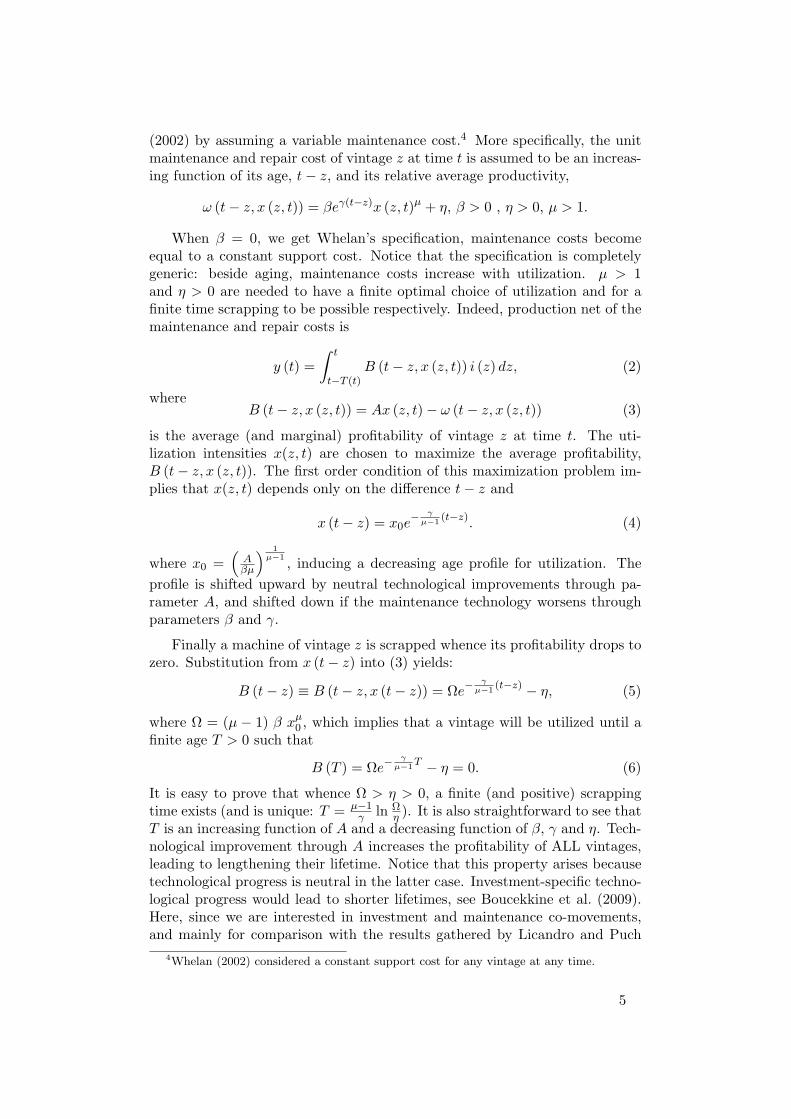
In this section, we run some numerical experiments using the analytical find-ings of the previous section. We choose to present the results of a non-anticipated, permanent and positive shock on the productivity parameters A.13
Before the shock, the parameters are chosen so that the long-run growth rateof the economy is between 2% and 3%, the ratio maintenance to investment isabout 50% as documented by McGrattan and Schmitz (1999), capital lifetimeis between 10 and 15 years, and an obsolescence rate between 1% and 3%, bothfigures being quite common in the literature.14 Figures 1 to 4 show an exampleof the optimal dynamics following a non-anticipated permanent 1% increasein the productivity parameter A for investment, maintenance, replacement in-vestment and the obsolescence rate. The first three variables are detrended inthe sense that each variable, say q(t), is reported as q(t) = q(t) e−gt, ∀t ≥ 0,where g is the long-run growth rate resulting from the permanent shock. Need-less to say, the value of machines’ lifetime, T , is adjusted from t = 0, since theA-shock also affects this variable.15 Last by not least, the figures are generatedwith an initial investment profile of the form ι(s) = ceg0s as anticipated in theprevious section. In the numerical illustration considered here, we set c = 1and g0 is the long-run growth rate of the economy before the A-shock, hereg0 = 2.54%.
Figures 1 and 2 give the optimal investment and maintenance dynamicsrespectively. Because initial investment profile is ι(s) = eg0s, detrended invest-ment satisfies:
limt→0−
ˆι(t) = limt→0−
e(g0−g)t = 1.
Figure 1 thus shows clearly that the permanent technological stimulus inducesa neat increase in (detrended) investment just after the shock relative to thecorresponding level just before the shock: Investment jumps at t = 0! This dis-continuity is quite common in the DDE literature (see Boucekkine et al., 2005).More importantly, Figure 1 captures very well the essential features of optimaladjustment in this kind of models: Investment is stimulated in the short andlong-run, though the long-run “multiplier” is smaller. In the middle, the dy-namics are much more persistent than in a model with homogeneous capitaldue to replacement dynamics. Due to these dynamics, which are themselvesinduced by the optimal constant lifetime of machines, convergence to the newbalanced growth paths is oscillatory (although the scale of the figures does notreflect this so neatly after t = 3T
2 ). This is again consistent with the availableAK theory with vintage capital. Figure 2 displays the optimal dynamics of
13We have also studied the consequences of shocks on the support cost, η.14More precisely, three parameters were fixed and four varied. The fixed parameters are:
β = 1, σ = 4 and ρ = 3%. The four varying parameters were: γ, A, η and µ.15In Figure 1 to 4, we have: A = 0.62 before the shock, γ = 1.89, η = 0.0296 and µ = 10.
This implies a long-run growth rate equal to 2.54% before the shock, and equal to 2.68%after the shock. The ratio maintenance expenditures to investment is close to 50%, and themachines’ lifetime is equal to 12.5 before the shock. The latter increases very slightly to 12.55years after the shock. The resulting obsolescence rate is equal to 1.30% before the shock.
20
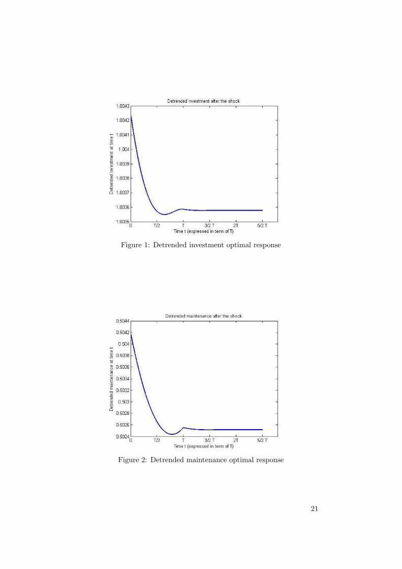
Figure 1: Detrended investment optimal response
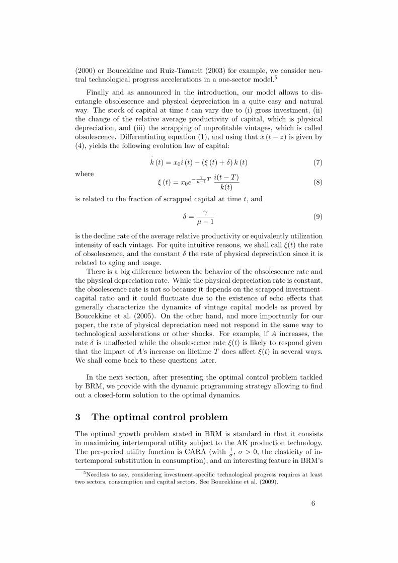
Figure 2: Detrended maintenance optimal response
21
capital maintenance. For a careful interpretation of the dynamics, the readershould note that given our parameterization
limt→0−
M(t) = 0.5008.
Figure 2 thus implies even the maintenance variable jumps at t = 0, which ismuch more surprising than the investment jump. Indeed, M(t) is not a controlvariable, and moreover, it is a weighted time integral of the investment profilefrom t to t−T , as reflected in equation (11). So why this jump? This jump oc-curs because the increase in the productivity parameter A changes the value ofoptimal lifetime from t = 0. Therefore the lower integration bound appearingin (11) gets modified, inducing the jump. More interestingly, one can noticethat investment and maintenance move in the same way. Maintenance goesup at t = 0 because capital lifetime increases (slightly) inducing a larger set ofvintages to maintain. The remaining maintenance dynamics are explained byinvestment dynamics given the integral law of motion (11).16 Overall, one cansee that optimal investment and maintenance patterns show a great degree ofcomplementarity, a property which we found to be robust to a wide variety ofshocks and initial conditions.17
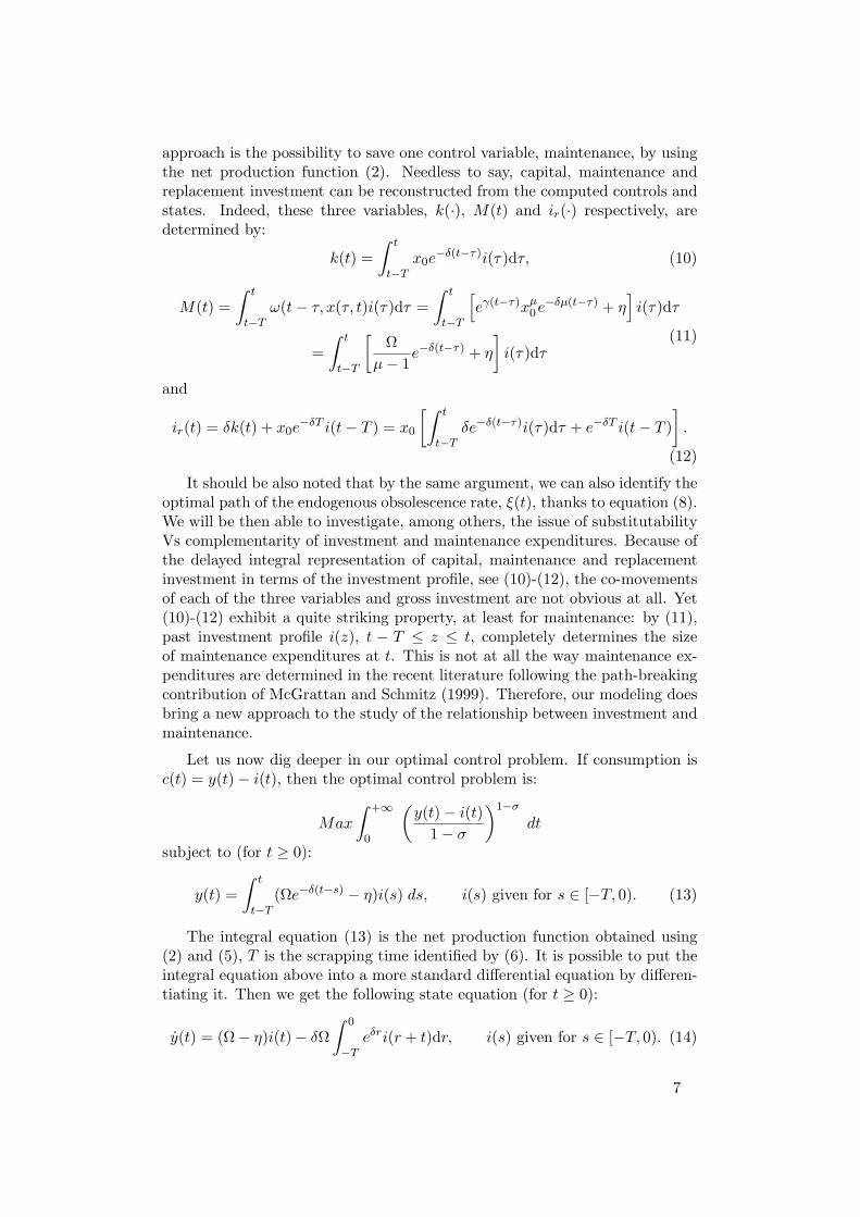
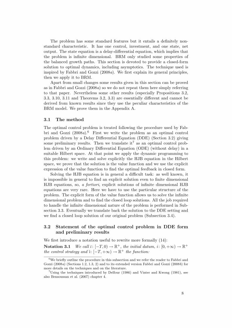
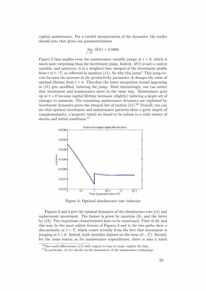
Figure 3: Optimal obsolescence rate behavior
Figures 3 and 4 give the optimal dynamics of the obsolescence rate ξ(t) andreplacement investment. The former is given by equation (8), and the latterby (12). Two important characteristics have to be mentioned. First of all, andthis may be the most salient feature of Figures 3 and 4, the two paths show adiscontinuity at t = T , which comes trivially from the fact that investment isjumping at t = 0. Indeed, both variables depend on the term i(t−T ). Second,for the same reason as for maintenance expenditures, there is also a much
16One could differentiate (11) with respect to time to make explicit the link.17In particular, we try shocks on the parameters of the maintenance technology.
22
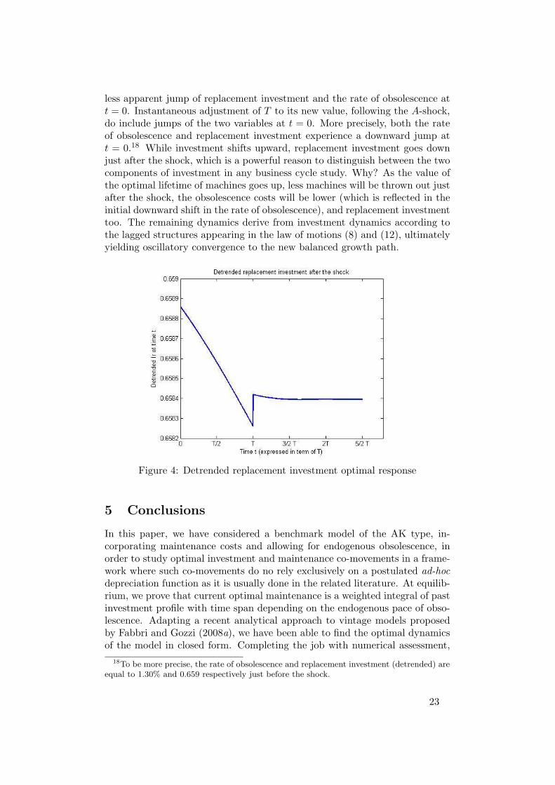
less apparent jump of replacement investment and the rate of obsolescence att = 0. Instantaneous adjustment of T to its new value, following the A-shock,do include jumps of the two variables at t = 0. More precisely, both the rateof obsolescence and replacement investment experience a downward jump att = 0.18 While investment shifts upward, replacement investment goes downjust after the shock, which is a powerful reason to distinguish between the twocomponents of investment in any business cycle study. Why? As the value ofthe optimal lifetime of machines goes up, less machines will be thrown out justafter the shock, the obsolescence costs will be lower (which is reflected in theinitial downward shift in the rate of obsolescence), and replacement investmenttoo. The remaining dynamics derive from investment dynamics according tothe lagged structures appearing in the law of motions (8) and (12), ultimatelyyielding oscillatory convergence to the new balanced growth path.
Figure 4: Detrended replacement investment optimal response
5 Conclusions
In this paper, we have considered a benchmark model of the AK type, in-corporating maintenance costs and allowing for endogenous obsolescence, inorder to study optimal investment and maintenance co-movements in a frame-work where such co-movements do no rely exclusively on a postulated ad-hocdepreciation function as it is usually done in the related literature. At equilib-rium, we prove that current optimal maintenance is a weighted integral of pastinvestment profile with time span depending on the endogenous pace of obso-lescence. Adapting a recent analytical approach to vintage models proposedby Fabbri and Gozzi (2008a), we have been able to find the optimal dynamicsof the model in closed form. Completing the job with numerical assessment,
18To be more precise, the rate of obsolescence and replacement investment (detrended) areequal to 1.30% and 0.659 respectively just before the shock.
23
we found that investment and maintenance move in the same way in responseto neutral technological shocks, which suggest that they act as complementaryto each other, which seems to be consistent with data.
Deviating from AK framework for more comprehensive empirical work willof course disable the analytical approach mostly taken in this paper. Forexample, with less stylized Cobb-Douglas technologies as in Boucekkine et al.(2009), the involved state equations are no longer linear delay differential equa-tions, so that one can only resort to a full computational approach. Moreover,accounting for investment-specific technological progress will make the analy-sis of investment and maintenance co-movements even trickier. Indeed, whileaccelerations in neutral technical progress lengthen capital lifetime as shownin this paper, investment-specific technological progress tends rather to de-crease it (see again Boucekkine et al. (2009)). In a model with both formsof technological progress, investment and maintenance co-movements wouldtherefore depend a lot on the composition of technological progress and on thesensitivity of the scrapping decision to each form of technical progress. Thisgoes much beyond the scope of this paper. But precisely because the lattergeneral problem seems quite hard to address properly, we do believe that thebenchmark analysis provided in this article is a necessary step in this researchprogram.
A Appendix: Proofs
We start by proving the following lemma that will be used in the proof of Proposition3.2Lemma A.1 The function F1 defined in (20) is strictly increasing and strictlyconcave. Moreover F1(−∞) = −∞, F1(0) = 0, F1(+∞) = Ω
(1− e−δT
)and
F ′1(0) = Ωδ
(1− e−δT − δTe−δT
).
Proof. It is not difficult to see that, setting h(x) = 1− e−x − xe−x, we have
F ′1(z) =Ωδ
(δ + z)2h((δ + z)T ), if z 6= −δ and F ′1(z) =
12ΩδT 2, if z = −δ
(45)while, setting g(x) = −2h(x) + xh′(x) = −2 + 2e−x + 2xe−x + x2e−x we get
F ′′1 (z) =Ωδ
(δ + z)3g((δ+z)T ), if z 6= −δ and F ′′1 (z) = −1
3ΩδT 3, if z = −δ.
(46)Now by simple computations we can see that
h(x) > 0, ∀x ∈ R− 0 andg(x)x3
< 0, ∀x ∈ R− 0.
so the whole claim of the Lemma easily follows.
Proof of Proposition 3.2The first statement is an immediate consequence of Lemma A.1. Statement (i) followsobserving that F ′1(0) > 1 by Hypothesis 3.1 and F ′1(π) < 1 by the strict monotonicity
24
and concavity of F1.To prove (ii) we first observe that (20) can be rewritten, multiplying by δ + z 6= 0, as
z2 +[−Ω
(1− e−δT
)+ δ
]z + δΩe−δT − δΩe−(δ+z)T = 0. (47)
All complex roots of (20) are also roots of (47): they are at most countable andhave the form λk = ak ± ibk for two sequences of real numbers ak and bk.Now a characteristic root is non-simple if and only if it satisfies also the equa-tion 2z +
(−Ω((1− e−δT
)+ δ
)+ δΩTe−(δ+z)T = 0. Combining the two equations
we get that a non simple characteristic root z must solve the quadratic equation
z2 +[
2T − Ω
(1− e−δT
)+ δ
]z + δΩe−δT +
Ω((1−e−δT )−δ
T . This means that there areat most two complex conjugate non simple characteristic roots. 2
Proof of Proposition 3.3By Diekmann et al. (1995) page. 34 and the Proposition 3.2 it follows that the solutionof (19) is continuous on R+ and
yM (t) = o(eπt) + αeπt +N∑
j=1
pj(t)eλjt for t → +∞
where λj are the finitely many roots of the characteristic equation with real partexceeding π and pj are C-valued polynomial in t. Now we can easily see that thepart due to the trigonometric polynomial
∑Nj=1 pj(t)eλjt vanish because the solution
remain always positive, due to the following property: if the initial datum ι(·) is notidentically zero then yM (t) remains positive for all t. Indeed, the solution is continuousand its value in 0 is strictly positive. If there exists a first point t in which the solutionis zero it satisfies:
yM (t) =∫ t
(t−T )∧0
yM (s + t)(Ωeδs − η)ds +∫ 0
(t−T )∨0
ι(s + t)(Ωeδs − η)ds
but the right hand side of equation is strictly positive because t is the first positivepoint in which yM (t) = 0. 2
Proof of Theorem 3.2Thanks to Theorem 5.1 page 282 in Bensoussan et al. (2007) we know that a so-lution exists for all i(·) ∈ L2
loc([0, +∞);R) when the initial datum z is in N :=R× F (L2([−T, 0);R)). Moreover the same theorem ensures that having a weak solu-tion as defined in (28) is equivalent to having a solution in the following mild sense:x(·) in Π is a (mild) solution if, for all ψ ∈ D(A),
〈ψ, x(t)〉 =⟨etAψ, z
⟩+
∫ t
0
C(e(t−r)Aψ
)i(s)ds (48)
that gives, for all z1, z2 ∈ N and i(·) ∈ L2loc([0, +∞);R), (xz1,i − xz2,i) = etA∗(z1−z2).
Moreover it is easy to see that N is dense in M2 and, fixed i(·) ∈ L2loc([0, +∞);R),
given z ∈ M2 and zn ∈ N with znn→∞−−−−→M2
z, that xzn,i(·) converges in Π to a xz,i(·)that is the solution we were looking for. 2
Proof of Theorem 3.3First of all we prove that φ ∈ AFSι. We divide the proof in two steps.Step 1: We claim that
ddtxφ(t) = A∗xφ(t) + C∗(φ(xφ(t))), t > 0xφ(0) = z = (R(ι), F (ι)) (49)
has a unique solution in Π.To prove this first step we consider the solution i(·) of the following delay differentialequation
25
i(t) = (1− ν)
(∫ t
(t−T )i(s)(Ωe−δ(t−s) − η)ds
)− ν
∫ 0
−TeπsF (it)(s)ds
i(s) = ι ∀ s ∈ [−T, 0)(50)
that has an absolute continuous solution i on [0,+∞) (see for example Bensoussanet al. (2007) page 287 for a proof). Then we consider the equation
ddtx = A∗x + C∗(i(t)), t > 0x(0) = z = (R(ι), F (ι)). (51)
We know, thanks to Theorem 3.1, that the only solution in Π of (51) is x(t) :=(y(t), F (it)) for all t ≥ 0, where y(·) is the solution of
y(t) = C(it); (y(0), i0) = (R(ι), ι).
We claim that x(t) is solution of (49) indeed
φ(x(t)) = y(t)− ν
( ∫ 0
−T
eπsF (it)(s)ds + y(t))
(52)
and so (by (50):
φ(x(t)) = y(t) (1− ν) + i(t)− (1− ν)( ∫ t
(t−T )
i(s)(Ωe−δ(t−s) − η)ds
)
and by (51) we conclude that φ(x(t)) = i(t) for all t ≥ 0 and so x(·) = xφ(·) is asolution of (49) and is in Π. Moreover thanks to the linearity of φ it is easy to observethat xφ(·) is the unique solution in Π.Step 2: We claim that φ(xφ(·)) ∈ Iι.We have to prove that, for all t ≥ 0, φ(xφ(t)) = i(t) ∈ [0, x0
φ(t)]. First we prove
that i(t) ≥ 0, i.e. that ν(∫ 0
−Teπsx1
φ(t)(s)ds + x0φ(t)
)≤ x0
φ(t). By Step 1 we havexφ(t) = (R(it), F (it)) so, using the definitions of R and F and the Fubini Theoremwe get:
ν
( ∫ 0
−T
eπsx1φ(t)(s)ds + x0
φ(t))
= ν
( ∫ 0
−T
Ωit(r)(
eδr − e−δT
− δ
δ + πeδre(δ+π)r +
δ
δ + πeδre−(δ+π)T
)dr
)
≤ ν
( ∫ 0
−T
Ωit(r)((eδr − e−δT )
(1− δ
δ + πe−T (δ+π)
))dr
)
= ν(1− δ
δ + πe−(δ+π)T
)R(it) ≤ R(it) = x0
φ(t) (53)
where the last inequality follows by Hypothesis 3.3.We prove now that, for all t ≥ 0, i(t) ≤ x0
φ(t) i.e. that
ν(x0
φ(t) +∫ 0
−Teπsx1
φ(t)(s)ds)≥ 0. Using the expressions of R and F as above
we get
x0φ(t) +
∫ 0
−T
eπsx1φ(t)(s)ds = R(it) +
∫ 0
−T
eπsF (it)(s)ds=∫ 0
−T
Ωi(r + t)Φ(r)dr
where the function Φ: [−T, 0] → R is given by
Φ: r 7→ eδr − e−δT − δ
δ + πeδr
(e(δ+π)r − e−(δ+π)T
).
Now by elementary computation we can prove that Φ(−T ) = 0 and Φ(r) > 0 for allr ∈ (−T, 0]. Using that i(t) ≥ 0 for all t > −T we have the claim.
26
This concludes the proof of the fact that φ is an admissible strategy related to ι.The optimality can be proved using the same arguments used by Fabbri and Gozzi(2008a) in the proof of Theorem II.2.13. 2
Proof of Proposition 3.10It is enough to try the solution a0e
a1s in (42). We find:
a0ea1s =
( ∫ 0
−T
Ωe(δ+a1)rdr −∫ 0
−T
Ωea1re−δT dr
)a0e
a1s
(π − ρ
σπ
)
+a0ea1sν
∫ 0
−T
eπτ
∫ τ
−T
e−a1τδΩe(a1+δ)rdrdτ
then
1 = Σ(a1)def=
(Ω
1δ + a1
(1− e−(δ+a1)T )− Ωe−δT 1a1
(1− e−a1T ))(
π − ρ
σπ
)
+ν
∫ 0
−T
e(π−a1)τδΩ1
δ + a1(e(a1+δ)τ − e−(a1+δ)T )dτ
=(
Ω1
δ + a1(1− e−(δ+a1)T )− Ωe−δT 1
a1(1− e−a1T )
)(π − ρ
σπ
)
+νδΩ
δ + a1
(1
π + δ(1− e−(π+δ)T )− e−(a1+δ)T 1
π − a1(1− e−(π−a1)T )
).
We can see that, when g > 0,
lima1→−∞
Σ(a1) = +∞ lima1→+∞
Σ(a1) = 0
then there exists a a1 such that Σ(a1) = 1 and than such that a0ea1· is the a BGP
for all positive a0. But from Theorem 3.4 (since we need b0eb1s − a0e
a1s = Λegs forall s ≥ 0) we can deduce that the only possible choice for a BGP is that a1 = b1 = g,then Σ(g) = 1 and a0e
g· is a BGP for all positive a0. The related state evolution willbe y(s) = b0e
gs where b0 =∫ 0
−TΩ(eδs − e−δT )a0e
gsds. 2Proof of Proposition 3.11
We have only to use the definitions and results of other sections, to substitute ι(s) =ceg0s (s ∈ [−T, 0)) and to solve the integrals. In particular we have to use (27) for (i),(38) for (ii), (39) and (41) for (iii), and (44) for (iv). 2
References
Askenazy, P. and Le Van, C. (1999). A model of optimal growth strategy.Journal of economic theory, 85: 24–51.
Bensoussan, A., Da Prato, G., Delfour, M. C. and Mitter, S. K. (2007). Rep-resentation and control of infinite dimensional systems. Systems & Control:Foundations & Applications. second edn. Boston, MA. Birkhauser BostonInc.
Boucekkine, R., Del Rio, F. and Martinez, B. (2008). A vintage ak theory ofobsolescence and depreciation. Working Paper.
Boucekkine, R., del Rio, F. and Martinez, B. (2009). Technological progress,obsolescence, and depreciation. Oxford Econ. Pap., . to appear.
27
Boucekkine, R., Licandro, O., Puch, L. A. and del Rio, F. (2005). Vintagecapital and the dynamics of the AK model. J. Econ. Theory, 120(1): 39–72.
Boucekkine, R. and Ruiz-Tamarit, R. (2003). Capital maintenance and invest-ment: Complements or substitutes?. J. Econ., 78(1): 1–28.
Collard, F. and Kollintzas, T. (2000). Maintenance, utilization, and deprecia-tion along the business cycle. Centre for Economic Policy Research.
Delfour, M. C. (1986). The linear quadratic optimal control problem withdelays in the state and control variables: a state space approch. SIAM J. ofControl Optim., 24: 835–883.
Diekmann, O., Van Gils, S., Verduyn Lunel, S. and Walther, H. (1995). Delayequations. Springer, Berlin.
Fabbri, G. and Gozzi, F. (2008a). Solving optimal growth models with vintagecapital: The dynamic programming approach. J. Econ. Theory, 143(1): 331–373.
Fabbri, G. and Gozzi, F. (2008b). Vintage capital in the ak growthmodel: a dynamic programming approach. extended version. preprint.http://ideas.repec.org/p/pra/mprapa/2863.html.
Feldstein, M. S. and Rothschild, M. (1974). Towards an economic theory ofreplacement investment. Econometrica, pp. 393–423.
Kalaitzidakis, P. and Kalyvitis, S. (2004). On the macroeconomic implicationsof maintenance in public capital. J. Public Econ., 88(3-4): 695–712.
Kalaitzidakis, P. and Kalyvitis, S. (2005). New public investment and/or publiccapital maintenance for growth? the canadian experience. Econ. Inquiry,43(3): 586–600.
Kalyvitis, S. (2006). Another look at the linear q model: an empirical analysisof aggregate business capital spending with maintenance expenditures. Can.J. Econ., 39(4): 1282–1315.
Licandro, O. and Puch, L. (2000). Capital utilization, maintenance costs andthe business cycle. Ann. Econ. Statist., pp. 143–164.
Licandro, O., Puch, L. A. and Ruiz-Tamarit, J. R. (2001). Optimal growthunder endogenous depreciation, capital utilization and maintenance costs.Investigaciones Econ., 25(3): 543–559.
McGrattan, E. and Schmitz, J. (1999). Maintenance and repair: Too big toignore. Fed. Reserve Bank Minneapolis Quart. Rev., 23(4): 2–13.
Nickell, S. (1975). A closer look at replacement investment. J. Econ. Theory,10: 54–88.
28
Saglam, C. and Veliov, V. (2008). Role of Endogenous Vintage Specific Depre-ciation in the Optimal Behavior of Firms. Int. J. Econ. Theory, 4(3): 381–410.
Vinter, R. B. and Kwong, R. H. (1981). The infinite time quadratic controlproblem for linear system with state control delays: An evolution equationapproch. SIAM J. of Control Optim., 19: 139–153.
Whelan, K. (2002). Computers, obsolescence, and productivity. Rev. Econ.Statist., 84(3): 445–461.
29