sovereign debt and bank loans: complements or substitutes?

1

Sovereign debt and bank loans:

complements or substitutes?

Cai Liu

ICMA Centre

Henley Business School

University of Reading

Simone Varotto

ICMA Centre

Henley Business School

University of Reading

Abstract

We explore the relationship between bank’s sovereign debt holdings and lending to the

private sector in Eurozone banks over the subprime and sovereign debt crises and the recovery

period that followed. We find that small banks in distressed countries were not subject to (1)

the substitution effect between sovereign debt and bank loans witnessed in large banks, and (2)

the resulting lending restrictions. The implication is that a financial sector with smaller banks

may prove more resilient to financial crises. This supports incentives embedded in new banking

regulation that penalise bank size. On the other hand, our results suggest that cheap funding

provided through quantitative easing programmes has led to substantially higher exposure of

small banks to domestic sovereign debt. This reinforces the sovereign-bank “doom loop”

documented in larger institutions.

JEL Classification: G01, G10, G21, G28

Keywords: Bank Lending, Eurozone Crisis, Government Bonds, Sovereign Risk

2

1. Introduction

The European debt crisis erupted in the wake of the Great Recession in late 2009, and was

characterized by an environment of accelerating government debt levels and increasing

government bond yields. One of the main causes of the debt crisis is that several European

governments were forced to rescue troubled banks headquartered in their countries (Acharya

et al. 2014). Consequently, national debt burdens increased and public finances deteriorated

significantly (IMF 2009). Banks absorbed increasing levels of government debt which raises

the question of how bank lending is allocated between private and public borrowers and the

consequences of such allocation for economic growth. Two major hypotheses have been

developed to explain the relationship between bank’s sovereign debt holdings and loan growth.

The “moral suasion” channel documented by Becker and Ivashina (2014), Ongena et al. (2016)

and De Macro and Machiavelli (2016) suggests that when sovereign risk increases and

government financing becomes more costly, governments may persuade the local financial

sector (especially large domestic banks) to absorb more government debt. If the financial sector

cannot raise additional funds to purchase government debt, these purchases may be made at

the expense of other investments e.g. retail and corporate loans. In contrast, as suggested by

Acharya and Steffen (2015), Acharya et al. (2016), and Buch et al. (2016), the “carry-trade”

and “risk-shifting” hypotheses can also explain this crowding-out effect. Additionally, given

the capital treatment of sovereign debt, banks may realise higher yields and benefit from lower

regulatory capital by shifting from bank loans to risky government debt (Acharya and Steffen,

2015). Riskier banks may even take this risk-shifting strategy as a bet on their own survival

(Diamond and Raja 2011; Broner et al 2014; Acharya and Steffen 2015; Crosignani 2015;

Drechsler et al 2016). A further link between sovereign debt exposure and bank loans may arise

as a result of the marking to market of government debt as discussed by De Macro (2016) and

3

Altavilla et al. (2016). Specifically, when sovereign bonds depreciate as credit spreads rise,

banks book losses that may further affect their ability to lend.

We contribute to the literature in three ways. First, when studying the substitution between

sovereign debt and bank loans, previous research mainly focuses on large banks. While it is

true that the overall market share of small banks may not be prominent,1 small banks are

believed to play a critical role in financing small businesses in the economy, and their

decentralized lending structure gives them an important advantage (Sapienza 2002; Berger et

al. 2005; Mian 2008). For these reasons we broaden our sample to include small banks and

provide an extensive comparison of the determinants of bank lending in small and large

institutions. This is particularly relevant in the light of new bank regulation that penalises large

banks (i.e. through capital add-ons applied to systemically important institutions as well as

ring-fencing) and may lead to a more distributed banking system with fewer large players and

more small to medium ones2. So far, Albertazzi et al (2014), with a sample of Italian banks, is

the only paper we are aware of that compares large and small banks when looking at the

interaction between sovereign debt and bank lending. They find that large banks are more

affected by sovereign risk changes. Our paper differs from theirs in several respects: (1) while

Albertazzi et al (2014) focus on sovereign risk alone we also take into account bank specific

exposures to sovereign debt from a rich database sourced from the European Banking Authority

(for large banks) and BvD’s Bankscope (for both large and small banks). This enables us to

capture cross-sectional variations in sovereign exposures which we find to be highly significant

in explaining bank lending patterns; (2) we extend our analysis beyond the Italian market to

include a broad sample of Eurozone banks, (3) our sample period includes the peak of the

1 In our sample, the aggregated loan provided by small banks is around 10% of the total, and aggregated sovereign debt exposure held by small banks is around 7%. 2 Downsizing may also result in the forced segregation of trading from lending operations in banks. Provisions to ring-fence risky activities were included in the 2010 Dodd-Frank Wall Street Reform and Consumer Protection Act in the US, the UK’s 2011 "Vickers Report" and the EU’s “Liikanen Report” on Bank Structural Reform.

4

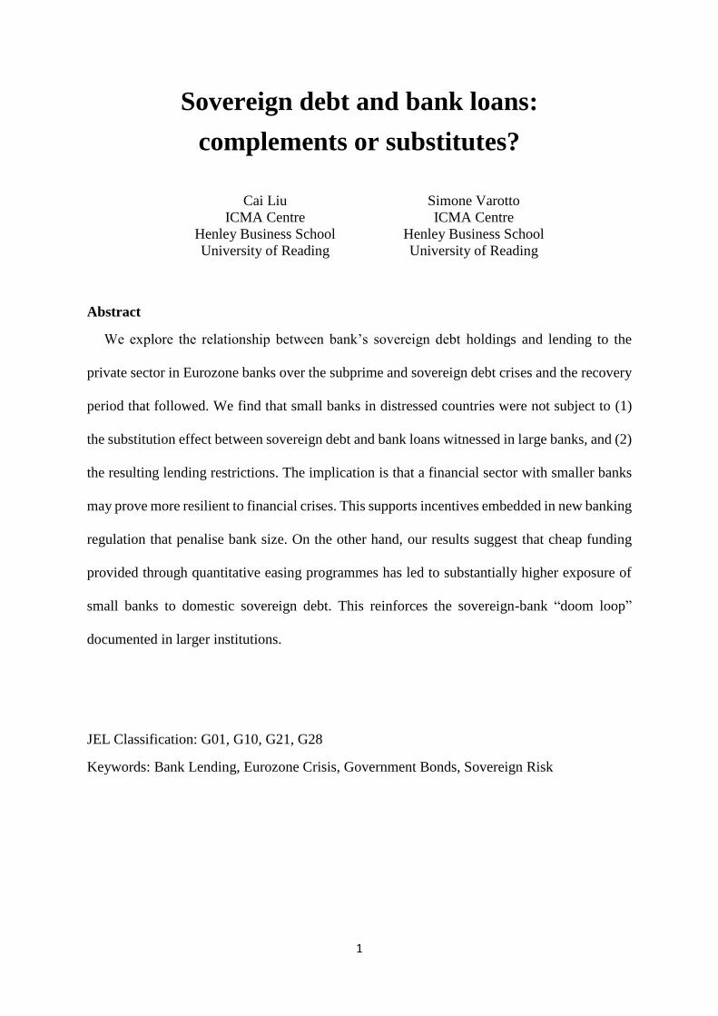
sovereign debt crisis and the following recovery phase which are characterised by a remarkable

growth in small banks’ exposure to sovereign debt especially in peripheral countries (see Figure

1). This growth takes place from 2011, which is right after the sample period (1991-2011)

covered by Albertazzi et al (2014). It is conceivable that their conclusions may partly be driven

by the fact that small banks were much less exposed to sovereign debt securities in their

observation period. Instead we show that small banks’ sovereign holdings may have a

significant impact on their loan growth.

Second, in addition to the substitution effect discussed in the literature (Becker and Ivashina

2014; Gennaioli et al. 2014; Popov and Van Horen 2014; De Macro 2016; Abbassi et al. 2016;

Altavilla et al. 2016), we also find a complementarity effect where sovereign debt and bank

loan growth are positively correlated3. We provide evidence that banks that have adequate

funding (either through the traditional channel of retail deposits, or through short-term

wholesale funding or cheap unconventional funds from central banks) and/or make substantial

gains in the sovereign bond portfolio, are more likely to increase both sovereign bond exposure

and loans to the private sector. This supports the notion that the ECB’s extraordinary liquidity

measures during the European sovereign debt crisis have helped to ease credit constraints in

the private sector (Daracq and De Santis, 2015 and Carpinelli and Crosignani, 2016).

Third, Becker and Ivashina (2014), Popov and Van Horen (2014), Acharya et al. (2016),

Altavilla et al. (2016) and De Marco (2016) measure bank lending with data on syndicated

loans (to large firms) or loans to non-financial corporations. By combining loan data from

BvD’s Bankscope (bank-level) and ECB Statistical Data Warehouse (country-level), we are

able to measure bank lending as total loans to the non-financial private sector, which includes

both non-financial corporations and households. This way we can explore more

3 The results of Altavilla et al. 2016 also observe a similar phenomenon when, in the recovery phase of the sovereign debt crisis decreasing bond yields generate capital gains in banks’ government bond portfolios which may help loan expansion.

5

comprehensively the relationship between banks’ sovereign bond exposure and their total

lending.

Our work relates more broadly to the literature on the sovereign-bank “doom loop”, that is,

the destabilising link generated by potential default risk spillovers between banks and

sovereigns through banks’ government bond holdings (Cooper and Nikolov (2013), Farhi and

Tirole (2014), Acharya et al. 2014 and Brunnermeier et al. (2016)). We observe that cheap

funding provided by the ECB may have contributed to a dramatic increase in sovereign debt

holdings in the banking sector which may exacerbate doom loop effects. This may have serious

financial stability implications in case of future shocks to sovereign debt yields.

Another main finding relates to the evidence that the crowding-out effect of sovereign debt

holdings is more pronounced for large banks in peripheral countries if they are state-owned.

So it appears that moral suasion may be particularly strong in stressed countries and in

institutions where the government can more directly influence investment policies.

The paper proceeds as follows. In section 2, we present the data and some stylized facts. In

section 3, we introduce our empirical model. In sections 4 and 5 we discuss the results and

provide robustness tests. Section 6 concludes the paper.

2. Data and Stylized Facts

This section describes our data and illustrates some stylized facts about the relationship

between sovereign debt holdings and loan growth in Eurozone banks. Our sample covers “core

countries” (Austria, Belgium, Germany, France, and Netherlands) and “peripheral countries”

(Greece, Ireland, Italy, Portugal and Spain) in the Eurozone and the analysis is carried out for

the period 2007-2015.

Sovereign debt exposure data are collected from two data sources. First, we use a novel

database of country specific sovereign exposures for a sample of large European banks that

6

participated in the stress tests and risk assessments conducted by the European Banking

Authority (EBA) over the period from March 2010 to June 20154. The number of banks varies

among different tests, but according to the EBA, each test covers at least 60% of total EU

banking assets. These data constitute the “large bank” sample in our analysis. A bank is

included if it is from any of the ten countries mentioned above and participated at least twice

in any of the EBA tests. This leaves us with 94 banks. Then, we use end of year data5 for

government bond exposures which exclude loans and advances to governments6. This way we

could make the data more consistent with another source for sovereign data, BvD Bankscope,

which only has information on sovereign bond exposures.

In order to include more banks and extend the sample period, we use the BvD Bankscope

database as a second source for banks’ government bond exposures. However, the data from

Bankscope is less detailed, which only gives the total government debt of a bank with no

counterparty breakdowns as in the EBA database. We include all banks from those 10 countries,

and then extract the small bank sample. A bank is qualified as “small” if its average asset is

lower than the 80% percentile of all non-EBA banks in its home country. All the other bank-

level variables for both large and small banks are from BvD Bankscope. We use Bankscope

data for the analysis in Section 4 (large banks vs small banks) and EBA data for Section 5

(large banks only).

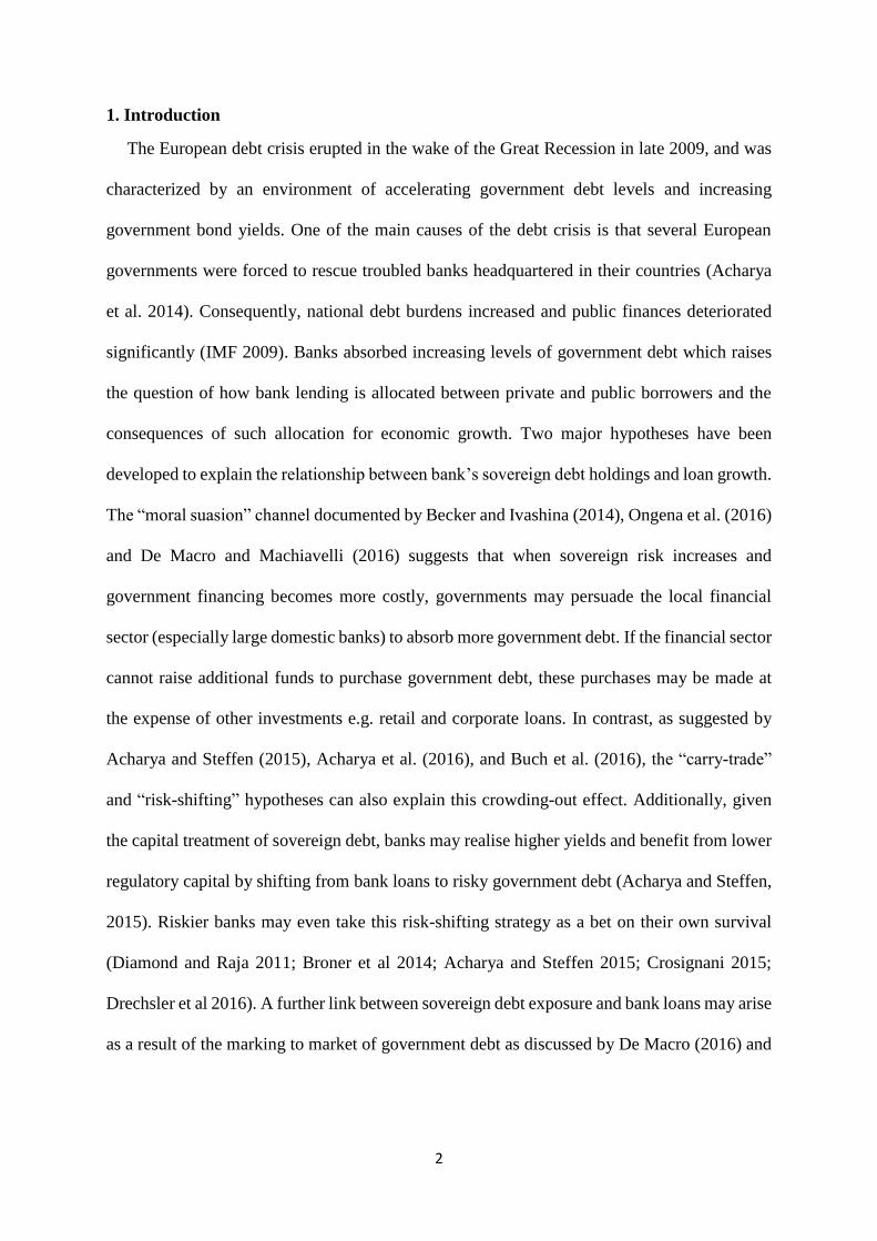
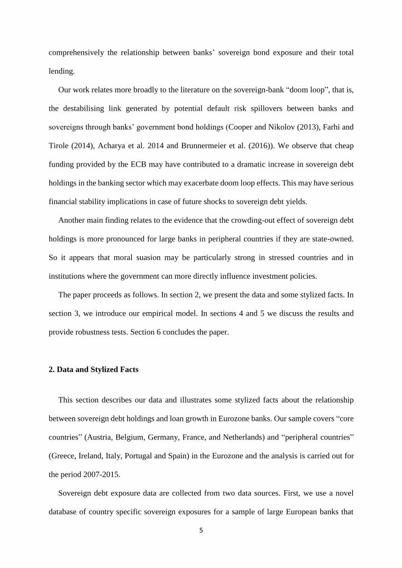
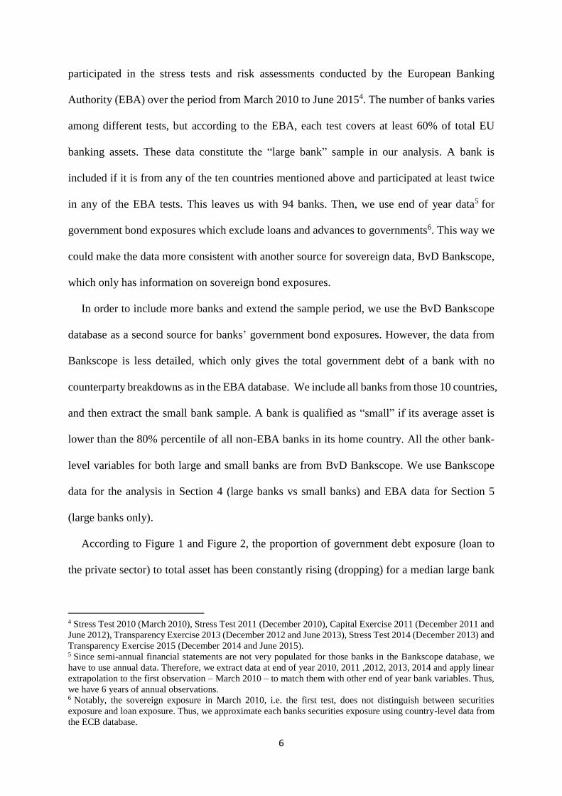
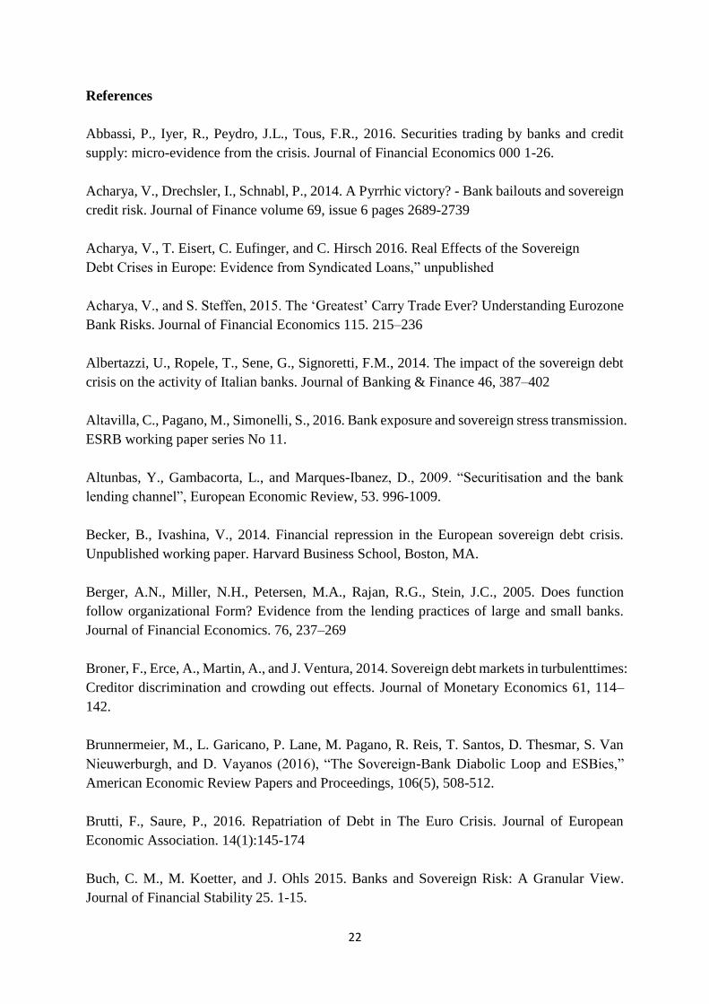
According to Figure 1 and Figure 2, the proportion of government debt exposure (loan to

the private sector) to total asset has been constantly rising (dropping) for a median large bank

4 Stress Test 2010 (March 2010), Stress Test 2011 (December 2010), Capital Exercise 2011 (December 2011 and

June 2012), Transparency Exercise 2013 (December 2012 and June 2013), Stress Test 2014 (December 2013) and

Transparency Exercise 2015 (December 2014 and June 2015). 5 Since semi-annual financial statements are not very populated for those banks in the Bankscope database, we

have to use annual data. Therefore, we extract data at end of year 2010, 2011 ,2012, 2013, 2014 and apply linear

extrapolation to the first observation – March 2010 – to match them with other end of year bank variables. Thus,

we have 6 years of annual observations. 6 Notably, the sovereign exposure in March 2010, i.e. the first test, does not distinguish between securities

exposure and loan exposure. Thus, we approximate each banks securities exposure using country-level data from

the ECB database.

7

in the peripheral countries. Such pattern is much more pronounced for a median small bank in

the peripheral countries. In contrast, both asset types are increasing marginally but steadily in

the small banks from core countries, and it seems that they barely hold government securities.

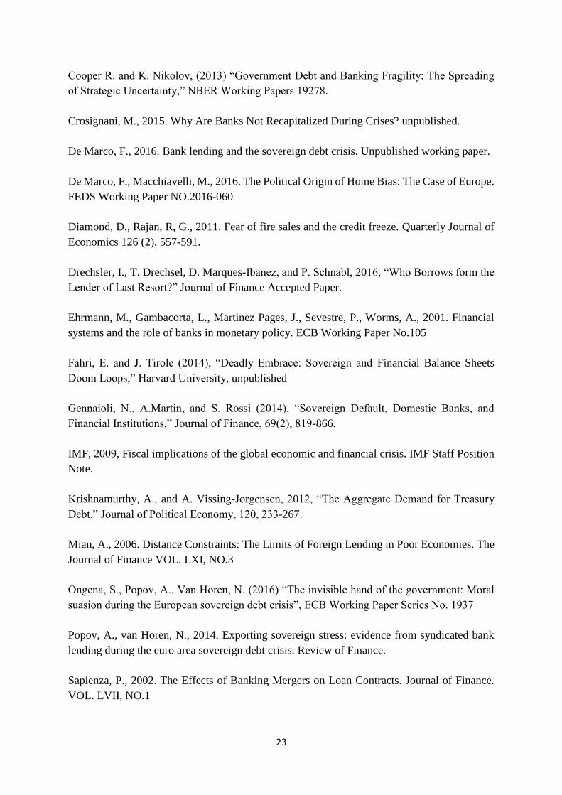
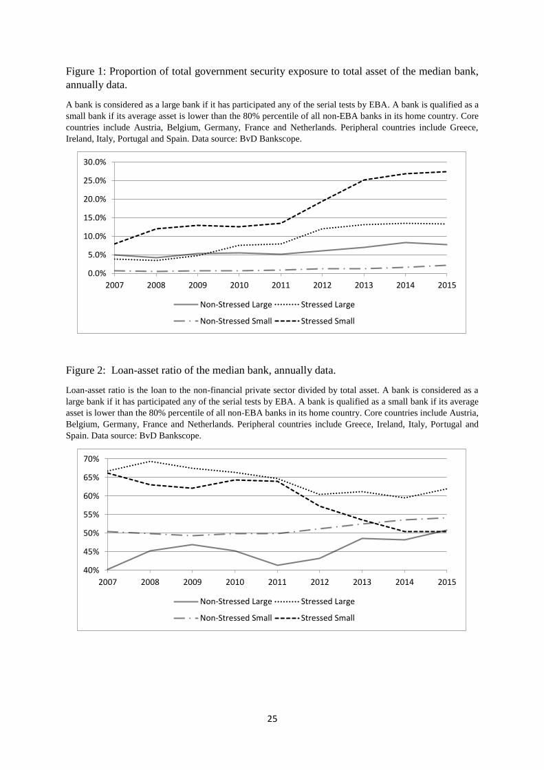
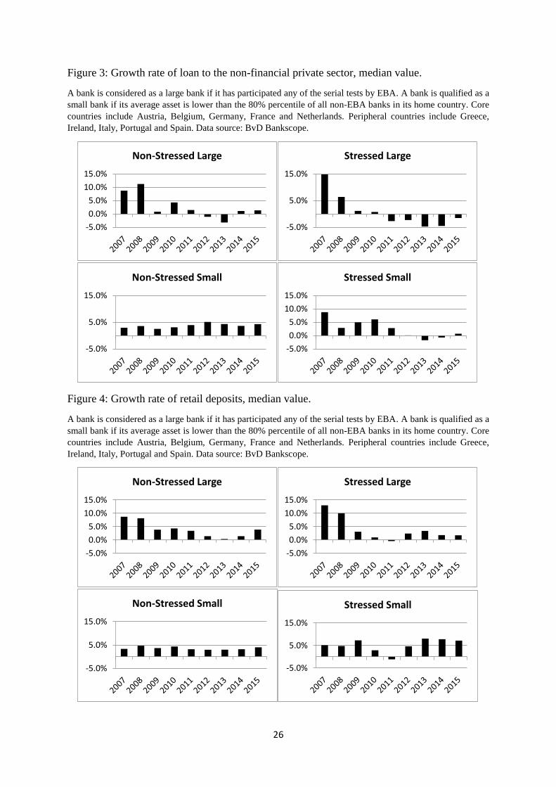
Interestingly, for small peripheral banks, their loan-asset ratio has been decreasing more

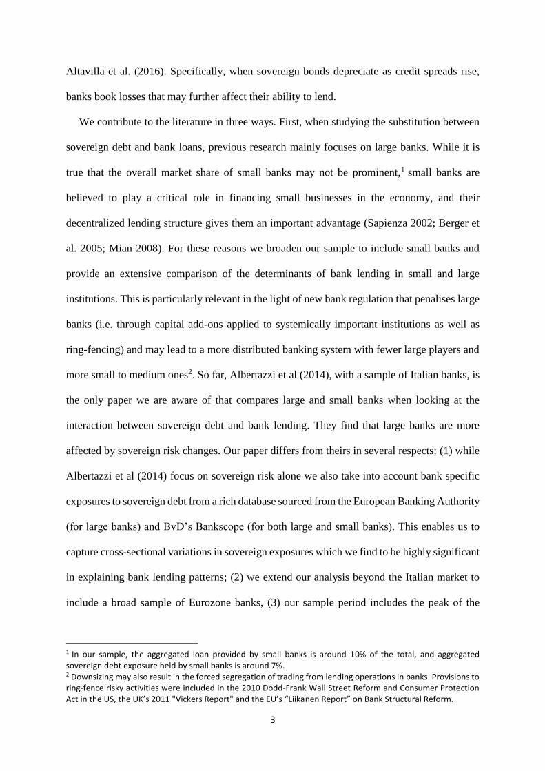
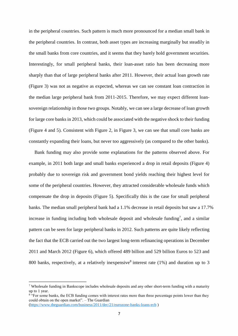
sharply than that of large peripheral banks after 2011. However, their actual loan growth rate

(Figure 3) was not as negative as expected, whereas we can see constant loan contraction in

the median large peripheral bank from 2011-2015. Therefore, we may expect different loan-

sovereign relationship in those two groups. Notably, we can see a large decrease of loan growth

for large core banks in 2013, which could be associated with the negative shock to their funding

(Figure 4 and 5). Consistent with Figure 2, in Figure 3, we can see that small core banks are

constantly expanding their loans, but never too aggressively (as compared to the other banks).

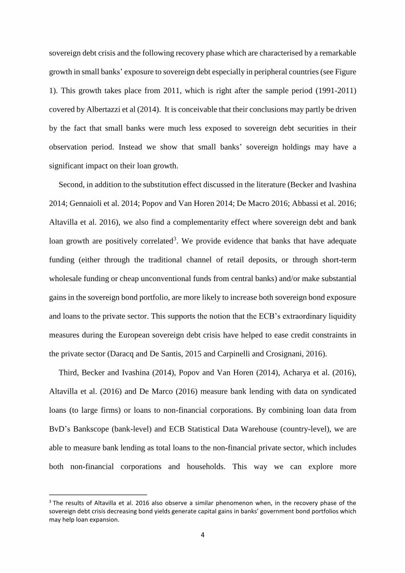
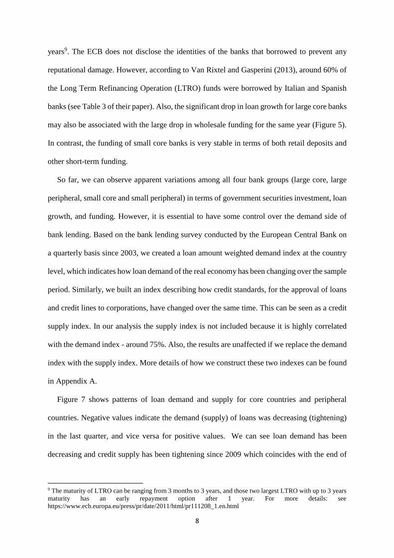
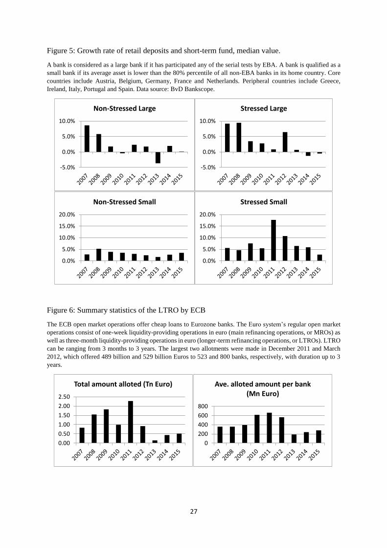
Bank funding may also provide some explanations for the patterns observed above. For

example, in 2011 both large and small banks experienced a drop in retail deposits (Figure 4)

probably due to sovereign risk and government bond yields reaching their highest level for

some of the peripheral countries. However, they attracted considerable wholesale funds which

compensate the drop in deposits (Figure 5). Specifically this is the case for small peripheral

banks. The median small peripheral bank had a 1.1% decrease in retail deposits but saw a 17.7%

increase in funding including both wholesale deposit and wholesale funding7, and a similar

pattern can be seen for large peripheral banks in 2012. Such patterns are quite likely reflecting

the fact that the ECB carried out the two largest long-term refinancing operations in December

2011 and March 2012 (Figure 6), which offered 489 billion and 529 billion Euros to 523 and

800 banks, respectively, at a relatively inexpensive8 interest rate (1%) and duration up to 3

7 Wholesale funding in Bankscope includes wholesale deposits and any other short-term funding with a maturity

up to 1 year. 8 “For some banks, the ECB funding comes with interest rates more than three percentage points lower than they

could obtain on the open market”. – The Guardian

(https://www.theguardian.com/business/2011/dec/21/eurozone-banks-loans-ecb )

https://www.theguardian.com/business/2011/dec/21/eurozone-banks-loans-ecb

8

years9. The ECB does not disclose the identities of the banks that borrowed to prevent any

reputational damage. However, according to Van Rixtel and Gasperini (2013), around 60% of

the Long Term Refinancing Operation (LTRO) funds were borrowed by Italian and Spanish

banks (see Table 3 of their paper). Also, the significant drop in loan growth for large core banks

may also be associated with the large drop in wholesale funding for the same year (Figure 5).

In contrast, the funding of small core banks is very stable in terms of both retail deposits and

other short-term funding.

So far, we can observe apparent variations among all four bank groups (large core, large

peripheral, small core and small peripheral) in terms of government securities investment, loan

growth, and funding. However, it is essential to have some control over the demand side of

bank lending. Based on the bank lending survey conducted by the European Central Bank on

a quarterly basis since 2003, we created a loan amount weighted demand index at the country

level, which indicates how loan demand of the real economy has been changing over the sample

period. Similarly, we built an index describing how credit standards, for the approval of loans

and credit lines to corporations, have changed over the same time. This can be seen as a credit

supply index. In our analysis the supply index is not included because it is highly correlated

with the demand index - around 75%. Also, the results are unaffected if we replace the demand

index with the supply index. More details of how we construct these two indexes can be found

in Appendix A.

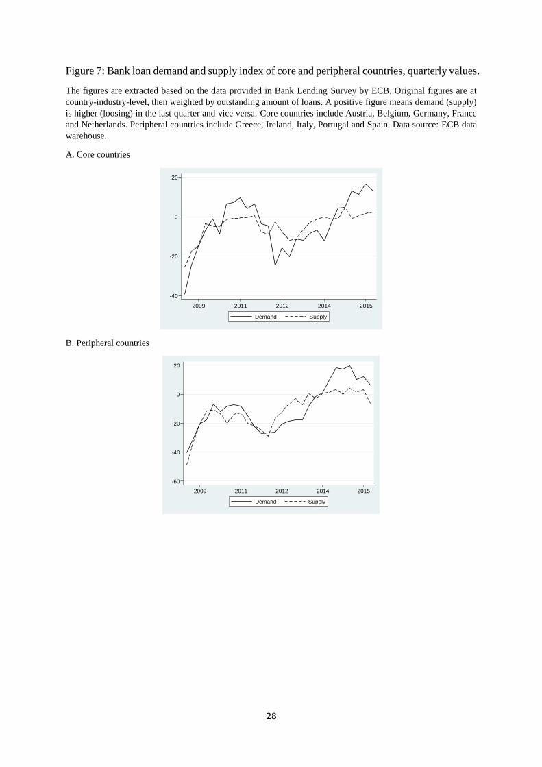
Figure 7 shows patterns of loan demand and supply for core countries and peripheral

countries. Negative values indicate the demand (supply) of loans was decreasing (tightening)

in the last quarter, and vice versa for positive values. We can see loan demand has been

decreasing and credit supply has been tightening since 2009 which coincides with the end of

9 The maturity of LTRO can be ranging from 3 months to 3 years, and those two largest LTRO with up to 3 years

maturity has an early repayment option after 1 year. For more details: see

https://www.ecb.europa.eu/press/pr/date/2011/html/pr111208_1.en.html

9

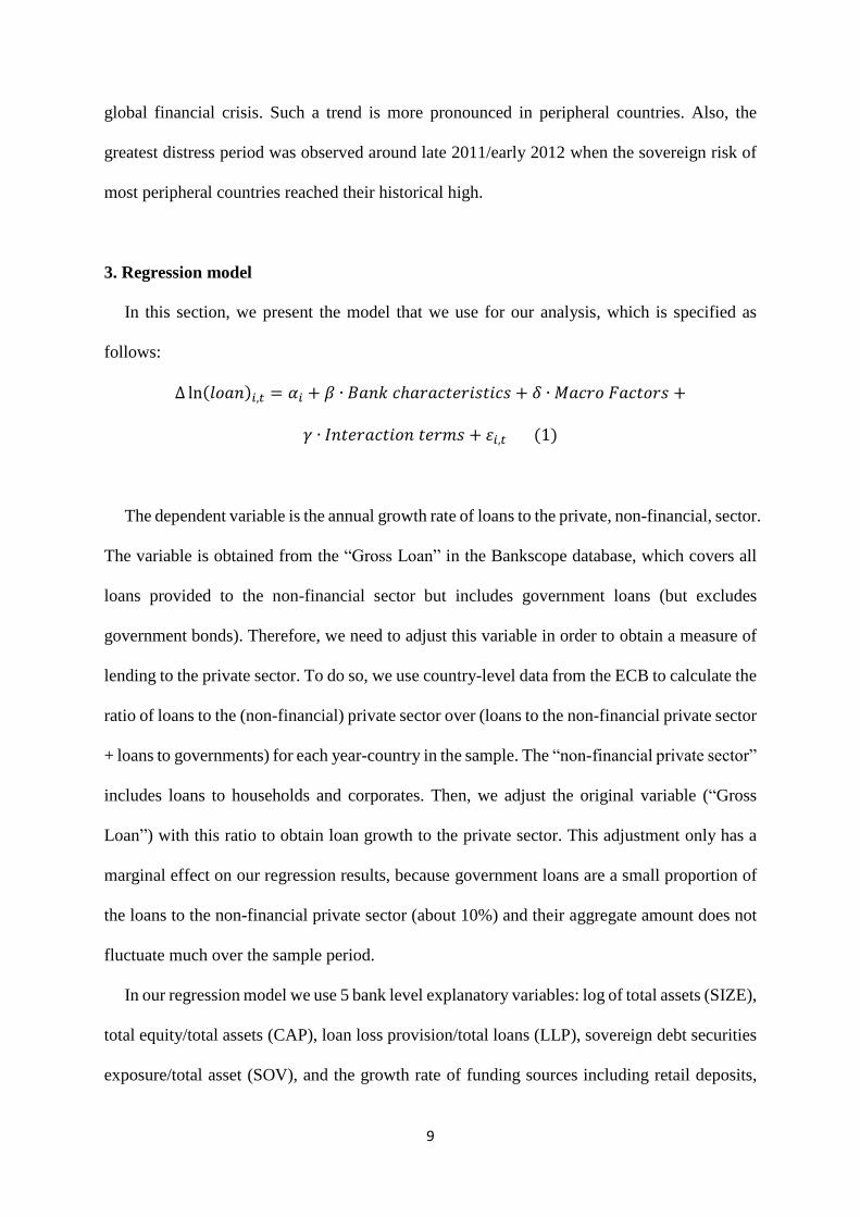
global financial crisis. Such a trend is more pronounced in peripheral countries. Also, the

greatest distress period was observed around late 2011/early 2012 when the sovereign risk of

most peripheral countries reached their historical high.

3. Regression model

In this section, we present the model that we use for our analysis, which is specified as

follows:

∆ ln(𝑙𝑜𝑎𝑛)𝑖,𝑡 = 𝛼𝑖 + 𝛽 ∙ 𝐵𝑎𝑛𝑘 𝑐ℎ𝑎𝑟𝑎𝑐𝑡𝑒𝑟𝑖𝑠𝑡𝑖𝑐𝑠 + 𝛿 ∙ 𝑀𝑎𝑐𝑟𝑜 𝐹𝑎𝑐𝑡𝑜𝑟𝑠 +

𝛾 ∙ 𝐼𝑛𝑡𝑒𝑟𝑎𝑐𝑡𝑖𝑜𝑛 𝑡𝑒𝑟𝑚𝑠 + 휀𝑖,𝑡 (1)

The dependent variable is the annual growth rate of loans to the private, non-financial, sector.

The variable is obtained from the “Gross Loan” in the Bankscope database, which covers all

loans provided to the non-financial sector but includes government loans (but excludes

government bonds). Therefore, we need to adjust this variable in order to obtain a measure of

lending to the private sector. To do so, we use country-level data from the ECB to calculate the

ratio of loans to the (non-financial) private sector over (loans to the non-financial private sector

+ loans to governments) for each year-country in the sample. The “non-financial private sector”

includes loans to households and corporates. Then, we adjust the original variable (“Gross

Loan”) with this ratio to obtain loan growth to the private sector. This adjustment only has a

marginal effect on our regression results, because government loans are a small proportion of

the loans to the non-financial private sector (about 10%) and their aggregate amount does not

fluctuate much over the sample period.

In our regression model we use 5 bank level explanatory variables: log of total assets (SIZE),

total equity/total assets (CAP), loan loss provision/total loans (LLP), sovereign debt securities

exposure/total asset (SOV), and the growth rate of funding sources including retail deposits,

10

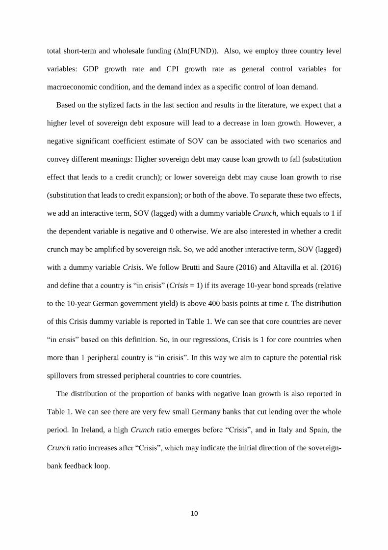
total short-term and wholesale funding (Δln(FUND)). Also, we employ three country level

variables: GDP growth rate and CPI growth rate as general control variables for

macroeconomic condition, and the demand index as a specific control of loan demand.

Based on the stylized facts in the last section and results in the literature, we expect that a

higher level of sovereign debt exposure will lead to a decrease in loan growth. However, a

negative significant coefficient estimate of SOV can be associated with two scenarios and

convey different meanings: Higher sovereign debt may cause loan growth to fall (substitution

effect that leads to a credit crunch); or lower sovereign debt may cause loan growth to rise

(substitution that leads to credit expansion); or both of the above. To separate these two effects,

we add an interactive term, SOV (lagged) with a dummy variable Crunch, which equals to 1 if

the dependent variable is negative and 0 otherwise. We are also interested in whether a credit

crunch may be amplified by sovereign risk. So, we add another interactive term, SOV (lagged)

with a dummy variable Crisis. We follow Brutti and Saure (2016) and Altavilla et al. (2016)

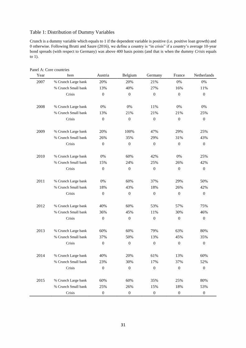
and define that a country is “in crisis” (Crisis = 1) if its average 10-year bond spreads (relative

to the 10-year German government yield) is above 400 basis points at time t. The distribution

of this Crisis dummy variable is reported in Table 1. We can see that core countries are never

“in crisis” based on this definition. So, in our regressions, Crisis is 1 for core countries when

more than 1 peripheral country is “in crisis”. In this way we aim to capture the potential risk

spillovers from stressed peripheral countries to core countries.

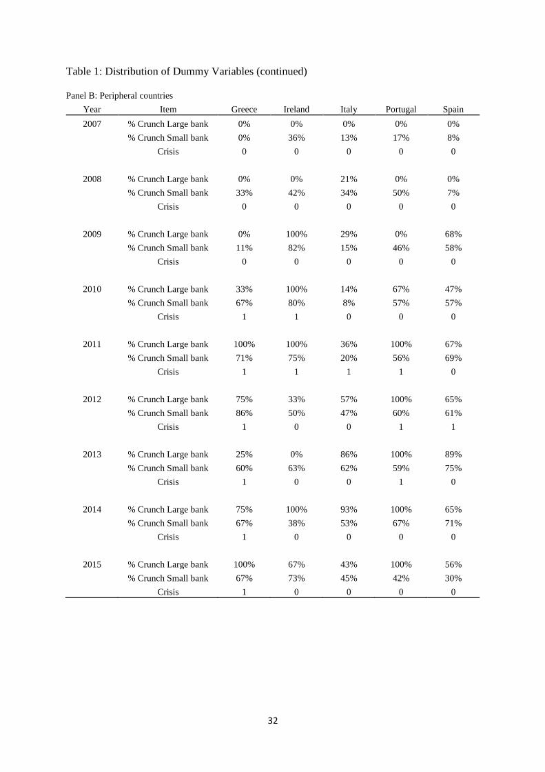
The distribution of the proportion of banks with negative loan growth is also reported in

Table 1. We can see there are very few small Germany banks that cut lending over the whole

period. In Ireland, a high Crunch ratio emerges before “Crisis”, and in Italy and Spain, the

Crunch ratio increases after “Crisis”, which may indicate the initial direction of the sovereign-

bank feedback loop.

11

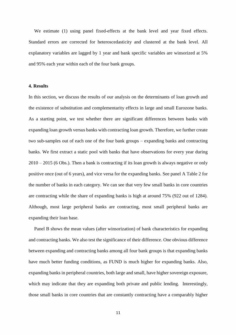
We estimate (1) using panel fixed-effects at the bank level and year fixed effects.

Standard errors are corrected for heteroscedasticity and clustered at the bank level. All

explanatory variables are lagged by 1 year and bank specific variables are winsorized at 5%

and 95% each year within each of the four bank groups.

4. Results

In this section, we discuss the results of our analysis on the determinants of loan growth and

the existence of substitution and complementarity effects in large and small Eurozone banks.

As a starting point, we test whether there are significant differences between banks with

expanding loan growth versus banks with contracting loan growth. Therefore, we further create

two sub-samples out of each one of the four bank groups – expanding banks and contracting

banks. We first extract a static pool with banks that have observations for every year during

2010 – 2015 (6 Obs.). Then a bank is contracting if its loan growth is always negative or only

positive once (out of 6 years), and vice versa for the expanding banks. See panel A Table 2 for

the number of banks in each category. We can see that very few small banks in core countries

are contracting while the share of expanding banks is high at around 75% (922 out of 1284).

Although, most large peripheral banks are contracting, most small peripheral banks are

expanding their loan base.

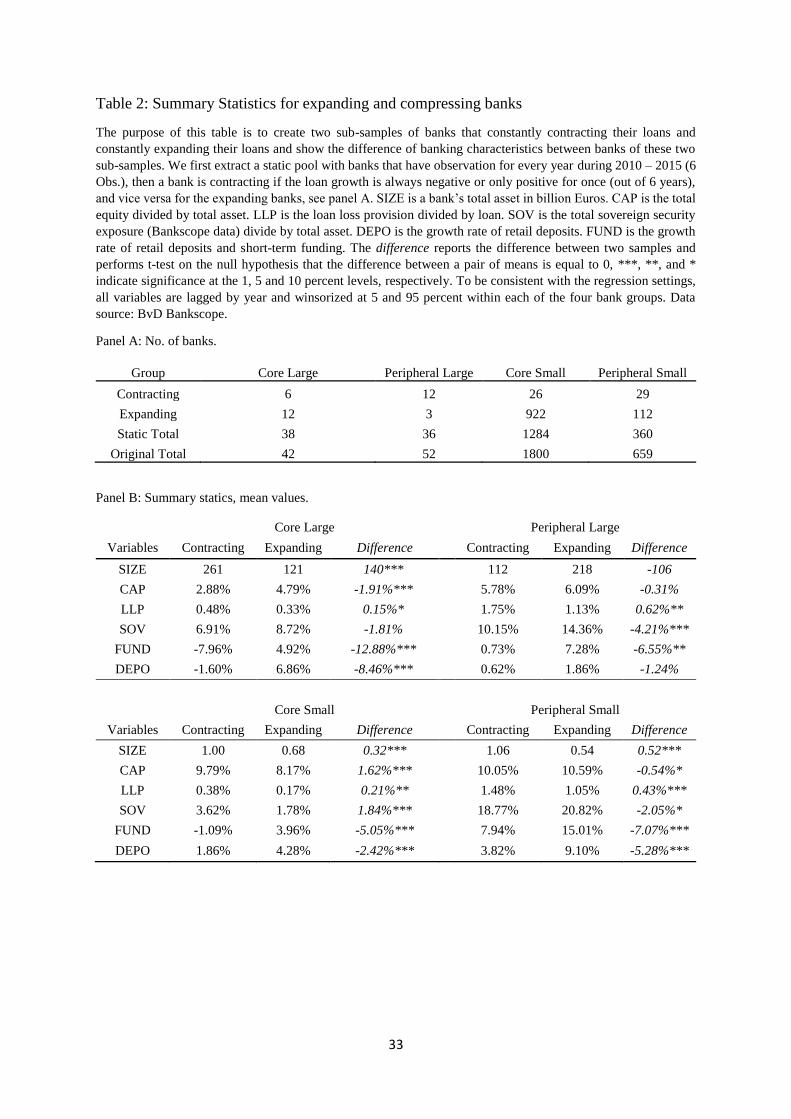
Panel B shows the mean values (after winsorization) of bank characteristics for expanding

and contracting banks. We also test the significance of their difference. One obvious difference

between expanding and contracting banks among all four bank groups is that expanding banks

have much better funding conditions, as FUND is much higher for expanding banks. Also,

expanding banks in peripheral countries, both large and small, have higher sovereign exposure,

which may indicate that they are expanding both private and public lending. Interestingly,

those small banks in core countries that are constantly contracting have a comparably higher

12

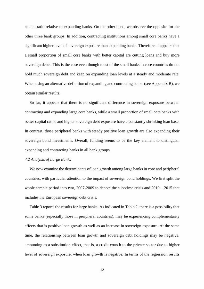
capital ratio relative to expanding banks. On the other hand, we observe the opposite for the

other three bank groups. In addition, contracting institutions among small core banks have a

significant higher level of sovereign exposure than expanding banks. Therefore, it appears that

a small proportion of small core banks with better capital are cutting loans and buy more

sovereign debts. This is the case even though most of the small banks in core countries do not

hold much sovereign debt and keep on expanding loan levels at a steady and moderate rate.

When using an alternative definition of expanding and contracting banks (see Appendix B), we

obtain similar results.

So far, it appears that there is no significant difference in sovereign exposure between

contracting and expanding large core banks, while a small proportion of small core banks with

better capital ratios and higher sovereign debt exposure have a constantly shrinking loan base.

In contrast, those peripheral banks with steady positive loan growth are also expanding their

sovereign bond investments. Overall, funding seems to be the key element to distinguish

expanding and contracting banks in all bank groups.

4.2 Analysis of Large Banks

We now examine the determinants of loan growth among large banks in core and peripheral

countries, with particular attention to the impact of sovereign bond holdings. We first split the

whole sample period into two, 2007-2009 to denote the subprime crisis and 2010 – 2015 that

includes the European sovereign debt crisis.

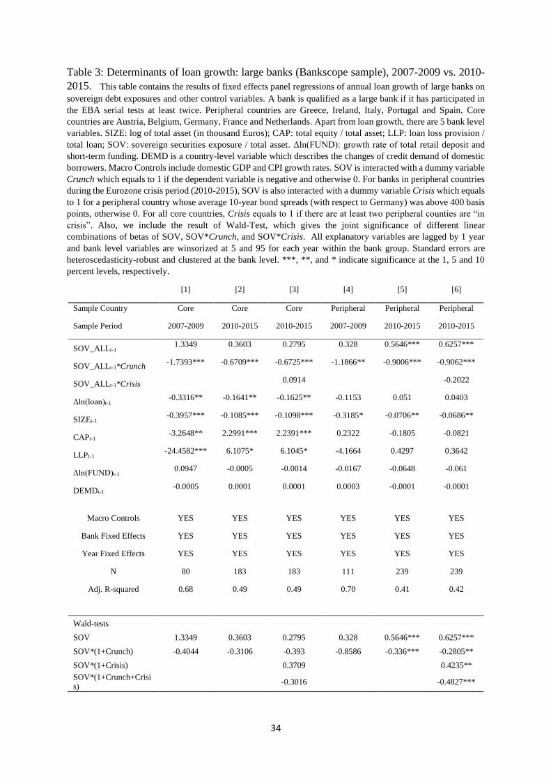
Table 3 reports the results for large banks. As indicated in Table 2, there is a possibility that

some banks (especially those in peripheral countries), may be experiencing complementarity

effects that is positive loan growth as well as an increase in sovereign exposure. At the same

time, the relationship between loan growth and sovereign debt holdings may be negative,

amounting to a substitution effect, that is, a credit crunch to the private sector due to higher

level of sovereign exposure, when loan growth is negative. In terms of the regression results

13

reported in Table 3 we then may expect the sign of the stand-alone SOV10 to be positive, and

the sign of SOV + SOV*Crunch 11 to be negative. The results of Wald-tests on linear

combinations of the regression coefficients can be found in the lower panel of Table 3. The

signs of the coefficients confirm our expectations, but they are only significant for large

peripheral banks during the sovereign debt crisis. Specifically, if loan growth is positive, a

higher level of sovereign exposure will contribute to a larger loan expansion. But, if a bank is

cutting its loan growth, a higher level of sovereign exposure will contribute to a larger loan

contraction. The substitution effect and complementarity effects found in large peripheral

banks during the period 2010-2015 are not only statistically significant but also economically

meaningful. Based on the result of Table 3 column 5, a one standard deviation increase in

sovereign exposure (5.26%), will add 2.97% to the annual loan growth rate, if loans are

growing. In contrast, the same amount of increase in sovereign exposure will deduct 1.77% 12

from the loan growth rate, if loans are decreasing.

Then, we look at how such impact can be changed when governments are in distress at some

points during the sample period. As described in Section 3, the dummy variable Crisis has

different meanings for core and peripheral countries. For peripheral countries, it indicates the

period when there is serious tensions domestically, featured by domestic sovereign bond yield

spread (over Germany) exceeding 400bps. For core countries, Crisis indicates the potential risk

spillovers originated from stressed peripheral countries, as the dummy equals to 1 if there is

more than 1 peripheral country “in crisis”. The results are reported in columns [3] and [6] of

10 The coefficient of the standalone SOV describes the impact of sovereign exposure on loan growth when loan is growing - positive growth rate. 11 The linear combination of the two coefficients describes the impact of sovereign exposure on loan growth when loan is decreasing – negative growth rate. 12 The 1.77% is obtained based on the regression result if we adjust regression [5] in table 3 by switch the interacted dummy from Crunch to Expand (which has the opposite definition) and keep everything else unchanged, thus the standalone SOV now measures the impact of sovereign exposure on loan growth if loan growth is negative. Given the size of one standard deviation of sovereign exposure, 5.26%, and the new coefficient of SOV -0.3360, then we get 1.7674% by multiplying the two figures.

14

Table 3. We do not spot any change in significance for large core banks (when compared to

columns [3] to [2]). However, we find that if the home country is “in crisis”, the substitution

effect will be more pronounced. This follows as the coefficient of SOV*(1+Crunch+Crisis) in

column 6 is much smaller than that of SOV*(1+Crunch), -0.48 vs. -0.28 and is more

statistically significant.

Consistent with Altunbas et al. (2009) and Ehrmann et al. (2001), the effect of size on loan

growth of large peripheral banks is negative. In comparison, CAP is significant only for large

core banks, but there is a switch in sign. Specifically, in the pre-sovereign crisis period, higher

capital has a negative impact on loan growth. But, after the outbreak of sovereign crisis, better

capitalization is associated to more loan growth. We can find a clue to such switch in Abbassi

et al (2016) who show that better capitalized banks are more likely to cut lending and use the

proceeds to buy risky debt before the start of the sovereign debt crisis. But when the sovereign

crisis begins, this strategy does not pay off anymore as sovereign bond prices start to fall. Then

a more intuitive positive relationship between capital and long growth emerges. Notably, loan

growth of large banks is not actively responding to (or significantly constrained by) its funding.

Finally, our country-level control variable for loan demand is never statistically significant13.

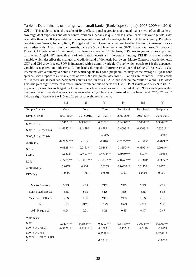
4.3 Analysis of Small Banks

We now conduct the same analysis for small banks in core and peripheral countries. Results

are reported in Table 4. If we look at the estimations of SOV and SOV*(1+Crunch) in columns

[1] and [4], we can see that small banks from both regions are subject to both substitution and

complementarity effect before the start of the Eurozone Crisis. This is surprising, as it is

contrary to our previous findings for large banks. The results are also economically meaningful.

For small core banks, one standard deviation increase (2.33%) in sovereign debt exposure can

13 We have tried different specifications of loan demand, e.g. by considering sector specific demands related to enterprises, mortgages and consumer credit, but without meaningful gains in significance.

15

add 1.74% to its annual loan growth rate if the bank is expanding its loans. And, it can reduce

loan growth by 2.18% and intensify the credit crunch further, if the bank is reducing its loans.

Therefore, such results may change the conventional idea that small banks are comparably less

involved in sovereign debt investment and their private lending business is less affected by

sovereign risk changes (Albertazzi et al. 2014).

Since the start of the Eurozone crisis, small core banks and small peripheral banks behave

differently. For small core banks, the coefficient of SOV dropped from 0.7477 to 0.3368

(columns [1] and [2] in Table 4) after the start of the Eurozone crisis, which means the

magnitude of the complementarity effect is smaller in 2010-2015 compared to 2007-2009

(given the fact that the standard deviation of SOV does not change much in these two periods).

As for the small banks in peripheral countries, the coefficient of SOV*(1+Crunch) in column

[5] is no longer statistically significant and close to zero, which means since the start of the

Eurozone crisis, they are no longer subject to substitution effect. Meanwhile, there is not much

difference in the coefficients of SOV in column [4] and [5], i.e. the complementarity effect

remains unchanged.

Also, small peripheral banks are still not subject to substitution effect even when their home

country is “in crisis”, as evidenced by the linear combination SOV*(1+Crunch+Crisis) in

column [6] of Table 4. We may find a clue for the absence of substitution effect if we consider

the evidence presented in Section 2 where we showed that small peripheral banks had

substantial funding increases in 2011 and 2012, which is quite likely due to large cheap loans

provided by the ECB. Therefore, holding more sovereign debt will not contribute to loan

contraction but it is positively associated with loan expansion. In other words, although small

peripheral banks increased their sovereign holdings dramatically (Figure 1), this does not

16

necessarily generate in fall in loan growth14. However, the availability of inexpensive funding

sources may greatly facilitate the complementarity effect, i.e. banks with adequate funding can

expand both their sovereign bond investments and loans to the private sector.

The negative and significant coefficient for CAP in the pre-sovereign debt crisis period may

be explained, as before, with a stronger credit contraction in banks that are better capitalised

(Abbassi et al. 2016) as they rebalance their investments towards traded securities (thus

reinforcing the substitution effect). Unlike for large core banks, such contraction is also present

for small core banks during the sovereign debt crisis period. This is probably due to the higher

capitalisation of the smaller core banks (see Table 2 Panel B) that may have sufficient capital

buffers to continue the above rebalancing even in the crisis. Finally, the degree of risk of the

loan portfolio as captured by loan loss provisions (LLP) is always an important concern among

all small banks where higher credit risk will lead to a decrease in loan growth.

5. Alternative mechanisms for substitution and complementarity effects

In this section, we further explore the sovereign-bank relationship and try to explain the

origins and mechanisms behind the substitution and complementarity effects. However, we are

able to do so only for the large banks, for which we have more detailed sovereign exposure

data from the EBA. However, the EBA sample only covers the period from 2010 to 2015.

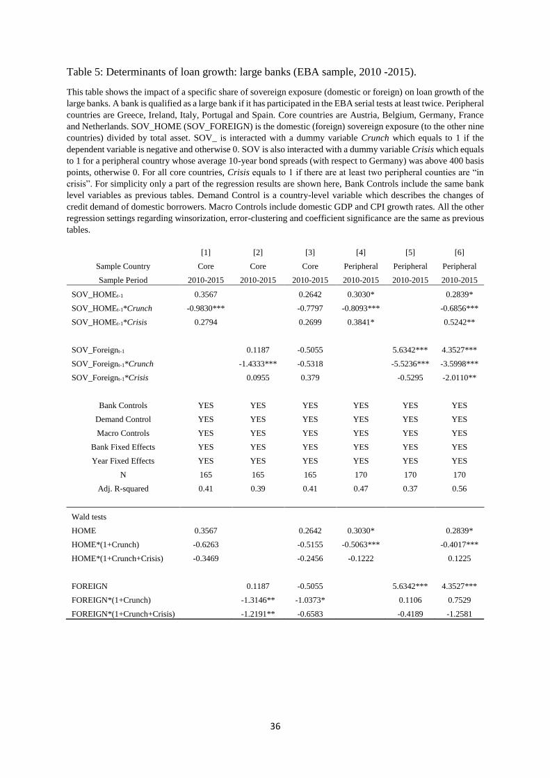
5.1 Domestic vs foreign sovereign debt holdings

Since the EBA database includes sovereign exposures held by each bank with details of the

country of issue, we can split the total sovereign holdings into domestic and foreign.15 Figure

14 In other words, loan contractions of small peripheral banks are more likely due to funding constraints rather than sovereign debt exposures. 15 As bond yields needed in later analysis are not consistently available for all EEA30 countries covered in the EBA sample, we only consider sovereign exposures to the 10 countries in our sample. Such restriction should not alter our findings, as the aggregated sovereign exposure held by our sample banks towards the included countries represents at least 85% of their total exposure to EEA30 countries.

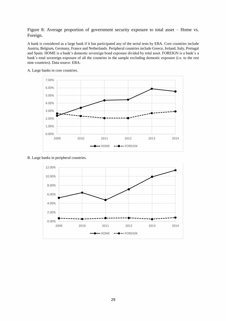
17

8 shows the average domestic and foreign government security exposure as a percentage of

total assets. It is quite obvious that large banks from both core and peripheral countries have

developed a stronger home bias in their sovereign bond portfolio. Indeed, the share of domestic

government debt exposure over total assets has more than doubled during the sample period.

Also, peripheral banks hold many more domestic sovereign bonds than foreign ones (the

exposure to the former being up to 13 times bigger) as compared to core banks. In contrast, in

2009 the average core bank was holding more foreign bonds than domestic ones. As a

consequence, we should expect a different impact of sovereign exposure on banks in the two

country groups.

Regression results are shown in Table 5. For large core banks, only the foreign sovereign

debt exposure may affect their loan growth and such effect only holds when there is a loan

contraction (see the coefficient estimation for FOREIGN*(1+Crunch) in columns [2] and [3]).

So the extension of our analysis enables us to detect a substitution effect that was not present

in Table 3 when all sovereign exposures where considered as an aggregate. As for the large

peripheral banks, in Section 4.2 we showed that they are subject to both substitution and

complementarity effects during 2010-2015. From columns [4]-[6] in Table 5, we can see that

the substitution effect is only originated from their domestic holdings. Also, the magnitude of

the substitution effect due to changes in domestic holdings is larger than that measured by total

sovereign holdings in Table 3. A one standard deviation increase in domestic (total) sovereign

exposure will lead to a deduction of 2.93% (1.47%) in loan growth rate, if loans are contracting.

On the other hand, for peripheral banks, when the home country is “in crisis” the substitution

effect disappears, contrary to results in in column [5] and [6] of Table 3. This is mainly due to

the fact that in the EBA sample is a very unbalanced panel and we may lose many critical

observations as compared to Bankscope sample. If we extract an identical set of bank-year

sample, the results are actually very similar using either EBA or Bankscope for the sovereign

18

data (see Appendix C16). However, complementarity effects can be traced to both domestic

and foreign sovereign exposures, and they are more closely associated with foreign sovereign

exposure even though it is a very small part on the balance sheet (on average always less than

1%, Figure 8).

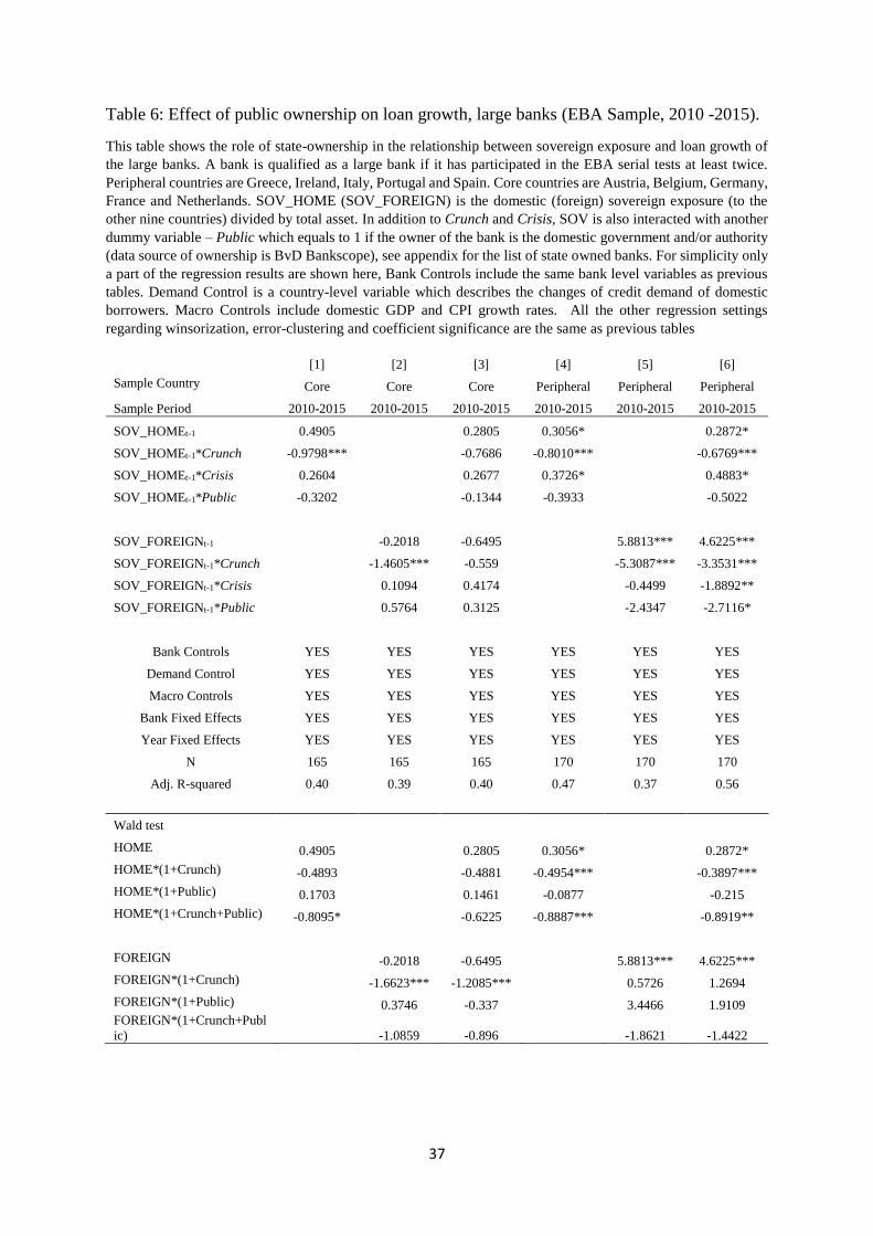
5.2 Further robustness tests

As suggested by Becker and Ivashina (2014), Ongena et al. (2016) and De Macro and

Machiavelli (2016), the substitution effect may be related to government pressure (the moral

suasion channel), that is, stressed governments have the incentive to force domestic banks to

absorb more of new debt issues. If the banks cannot raise additional funds to purchase

government debt, these purchases will probably be made at the expense of other investments

e.g. retail and corporate loans. To test this channel, we extract the ownership information of

the large banks from Bankscope and include an extra interaction term SOV_HOME with Public,

where Public is a dummy which equals 1 if the bank is a state-owned17 (see Appendix D for

the list of state-owned banks). The results in Table 6 do indicate the existence of the moral

suasion channel, especially for peripheral countries. Particularly, if we compare the coefficient

estimations of HOME*(1+Crunch) and HOME*(1+Crunch+Public) in columns [4] (or in [6]),

the coefficient increases markedly for publicly owned banks.

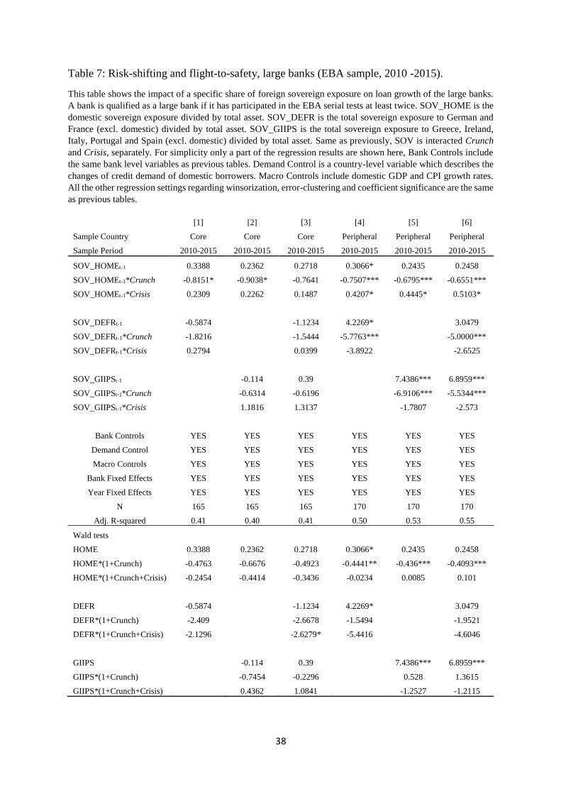
Also, the literature suggests that banks can realise higher yield but not face extra capital

requirements by investing more in risky government debt (Acharya and Steffen 2015; Acharya

et al. 2016; and Buch et al. 2016). In addition, banks may face liquidity shocks especially during

the crisis period. As a result, banks are willing to hold liquid assets such as safe sovereign

bonds at the expense of holding other assets (Krishnamurthy and Vissing-Jorgensen, 2012).

16 When we look at the result of SOV*(1+Crunch+Crisis) in [7] of Appendix C, it is not significant, as compared to that in [6] of Table 3. 17 In Bankscope, banks are defined as state-owned if the government holds more than 50% of the equity capital, we adopt the same definition.

19

We test both hypotheses by further breaking down foreign sovereign exposures into two parts.

Specifically, the safe part (labelled with DEFR) which equals to the sum of Germany and

France sovereign debt (when it is not domestic), and the risky part (labelled with GIIPS) which

equals to the sum of Greece, Ireland, Italy, Portugal and Spain sovereign debt (when it is not

domestic). As seen in Table 5, large banks in core countries are subject to substitution effect

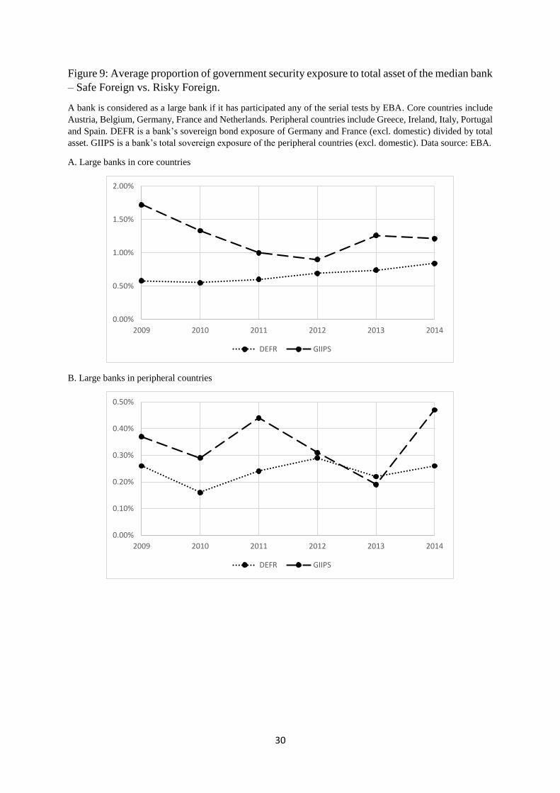
due to foreign sovereign exposures. Now, in Table 7 column [3] we can see that such

substitution can be largely driven by the incentive of flight-to-safety. Indeed, the only

significant coefficient is that of DEFR*(1+Crunch+Crisis). This means that during the period

when there are more than one peripheral countries “in crisis”, large core banks with higher

level of safe sovereign debt will have large loan contractions. This trend can also be observed

in Figure 9.A, where DEFR increases constantly through the whole period. In comparison,

consistent with the results in Table 5, foreign exposure, both safe and risky, is only responsible

for the complementarity effect in the large peripheral countries. In particular, it is mainly driven

by the risky sovereign exposure, which means high level of risky sovereign exposure may

indicate large credit expansion. Such results could indicate the existence of a very aggressive

yield-seeking behaviour, especially when we look at Figure 9.B which shows that the share of

GIIPS more than doubled in one year after 2013. Additionally, the complementarity effect can

also be attributed to the need of diversification across asset classes.

Lastly, there is a more direct mechanism for the sovereign exposure to have an impact on

loan growth, that is, through gains/losses of sovereign bond holdings. When sovereign bond

prices fall, banks suffer portfolio losses. If the fall is sever it may have an impact on the funds

available for lending. Of course, the effect can be symmetric, that is, profits in the sovereign

bond portfolio can lead to loan expansion. Therefore, the complementarity/substitution effects

could be explained by profit/losses made in government debt holdings. By following De Macro

(2016), we calculate the profit and loss of the sovereign debt portfolio. Specifically, we

20

consider P/L in all exposures, P/L in domestic exposure, and P/L in foreign exposures. The

details of the calculations are presented in Appendix E.1. Summary statistics of P/Ls can be

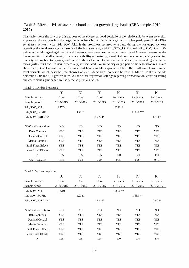
found in Appendix E.2. Regression results are shown in Table 8. We find that the P/L of foreign

sovereign bond holdings can affect loan growth in large core banks, while P/L of domestic

sovereign bond holdings is a key determinant for the loan growth for large peripheral banks.

6. Conclusion

By exploiting the impact of sovereign bond exposure on loan growth in both large and small

banks from core and peripheral Eurozone countries, we are able to bring a new perspective to

the literature. First, unlike the conventional idea that small banks are more oriented towards

traditional banking, we provide strong evidence that they were also very active in the sovereign

bond market. This had considerable impact on their own loan growth even before the start of

the Eurozone Crisis. Second, we find that high sovereign debt exposure can not only lead to

loan contraction (substitution effect), but also be associated with loan expansion

(complementarity effect). In this study we explore the causes of these two effects, and provide

a detailed discussion of the complex interactions behind them. The main implication of our

findings is that a financial sector with smaller banks may prove more resilient to financial crises.

This supports incentives embedded in new banking regulation that penalise bank size. On the

other hand, our results suggest that cheap funding provided through quantitative easing

programmes has led to substantially higher exposure of smaller banks to domestic sovereign

debt. This reinforces the sovereign-bank “doom loop” documented in larger institutions where

government distress can easily cause instability in the banking system and vice-versa.

Therefore, our research emphases the urgent need to finalise proposed reforms by the European

Commission and European Central Bank who seek to introduce a capital charge on sovereign

21

debt holdings and thus create an incentive for the banking sector to decrease their sovereign

exposures.18

18 See “Sovereign debt rule changes threaten EU bank finances”, The Financial Times, 8th June 2016,

22

References

Abbassi, P., Iyer, R., Peydro, J.L., Tous, F.R., 2016. Securities trading by banks and credit

supply: micro-evidence from the crisis. Journal of Financial Economics 000 1-26.

Acharya, V., Drechsler, I., Schnabl, P., 2014. A Pyrrhic victory? - Bank bailouts and sovereign

credit risk. Journal of Finance volume 69, issue 6 pages 2689-2739

Acharya, V., T. Eisert, C. Eufinger, and C. Hirsch 2016. Real Effects of the Sovereign

Debt Crises in Europe: Evidence from Syndicated Loans,” unpublished

Acharya, V., and S. Steffen, 2015. The ‘Greatest’ Carry Trade Ever? Understanding Eurozone

Bank Risks. Journal of Financial Economics 115. 215–236

Albertazzi, U., Ropele, T., Sene, G., Signoretti, F.M., 2014. The impact of the sovereign debt

crisis on the activity of Italian banks. Journal of Banking & Finance 46, 387–402

Altavilla, C., Pagano, M., Simonelli, S., 2016. Bank exposure and sovereign stress transmission.

ESRB working paper series No 11.

Altunbas, Y., Gambacorta, L., and Marques-Ibanez, D., 2009. “Securitisation and the bank

lending channel”, European Economic Review, 53. 996-1009.

Becker, B., Ivashina, V., 2014. Financial repression in the European sovereign debt crisis.

Unpublished working paper. Harvard Business School, Boston, MA.

Berger, A.N., Miller, N.H., Petersen, M.A., Rajan, R.G., Stein, J.C., 2005. Does function

follow organizational Form? Evidence from the lending practices of large and small banks.

Journal of Financial Economics. 76, 237–269

Broner, F., Erce, A., Martin, A., and J. Ventura, 2014. Sovereign debt markets in turbulenttimes:

Creditor discrimination and crowding out effects. Journal of Monetary Economics 61, 114–

142.

Brunnermeier, M., L. Garicano, P. Lane, M. Pagano, R. Reis, T. Santos, D. Thesmar, S. Van

Nieuwerburgh, and D. Vayanos (2016), “The Sovereign-Bank Diabolic Loop and ESBies,”

American Economic Review Papers and Proceedings, 106(5), 508-512.

Brutti, F., Saure, P., 2016. Repatriation of Debt in The Euro Crisis. Journal of European

Economic Association. 14(1):145-174

Buch, C. M., M. Koetter, and J. Ohls 2015. Banks and Sovereign Risk: A Granular View.

Journal of Financial Stability 25. 1-15.

23

Cooper R. and K. Nikolov, (2013) “Government Debt and Banking Fragility: The Spreading

of Strategic Uncertainty,” NBER Working Papers 19278.

Crosignani, M., 2015. Why Are Banks Not Recapitalized During Crises? unpublished.

De Marco, F., 2016. Bank lending and the sovereign debt crisis. Unpublished working paper.

De Marco, F., Macchiavelli, M., 2016. The Political Origin of Home Bias: The Case of Europe.

FEDS Working Paper NO.2016-060

Diamond, D., Rajan, R, G., 2011. Fear of fire sales and the credit freeze. Quarterly Journal of

Economics 126 (2), 557-591.

Drechsler, I., T. Drechsel, D. Marques-Ibanez, and P. Schnabl, 2016, “Who Borrows form the

Lender of Last Resort?” Journal of Finance Accepted Paper.

Ehrmann, M., Gambacorta, L., Martinez Pages, J., Sevestre, P., Worms, A., 2001. Financial

systems and the role of banks in monetary policy. ECB Working Paper No.105

Fahri, E. and J. Tirole (2014), “Deadly Embrace: Sovereign and Financial Balance Sheets

Doom Loops,” Harvard University, unpublished

Gennaioli, N., A.Martin, and S. Rossi (2014), “Sovereign Default, Domestic Banks, and

Financial Institutions,” Journal of Finance, 69(2), 819-866.

IMF, 2009, Fiscal implications of the global economic and financial crisis. IMF Staff Position

Note.

Krishnamurthy, A., and A. Vissing-Jorgensen, 2012, “The Aggregate Demand for Treasury

Debt,” Journal of Political Economy, 120, 233-267.

Mian, A., 2006. Distance Constraints: The Limits of Foreign Lending in Poor Economies. The

Journal of Finance VOL. LXI, NO.3

Ongena, S., Popov, A., Van Horen, N. (2016) “The invisible hand of the government: Moral

suasion during the European sovereign debt crisis”, ECB Working Paper Series No. 1937

Popov, A., van Horen, N., 2014. Exporting sovereign stress: evidence from syndicated bank

lending during the euro area sovereign debt crisis. Review of Finance.

Sapienza, P., 2002. The Effects of Banking Mergers on Loan Contracts. Journal of Finance.

VOL. LVII, NO.1

24

Van Rixtel, A., Gasperini, G., 2013. Financial crises and bank funding: recent experience in

the euro area. BIS Working Paper No 406

25

Figure 1: Proportion of total government security exposure to total asset of the median bank,

annually data.

A bank is considered as a large bank if it has participated any of the serial tests by EBA. A bank is qualified as a

small bank if its average asset is lower than the 80% percentile of all non-EBA banks in its home country. Core

countries include Austria, Belgium, Germany, France and Netherlands. Peripheral countries include Greece,

Ireland, Italy, Portugal and Spain. Data source: BvD Bankscope.

Figure 2: Loan-asset ratio of the median bank, annually data.

Loan-asset ratio is the loan to the non-financial private sector divided by total asset. A bank is considered as a

large bank if it has participated any of the serial tests by EBA. A bank is qualified as a small bank if its average

asset is lower than the 80% percentile of all non-EBA banks in its home country. Core countries include Austria,

Belgium, Germany, France and Netherlands. Peripheral countries include Greece, Ireland, Italy, Portugal and

Spain. Data source: BvD Bankscope.

0.0%

5.0%

10.0%

15.0%

20.0%

25.0%

30.0%

2007 2008 2009 2010 2011 2012 2013 2014 2015

Non-Stressed Large Stressed Large

Non-Stressed Small Stressed Small

40%

45%

50%

55%

60%

65%

70%

2007 2008 2009 2010 2011 2012 2013 2014 2015

Non-Stressed Large Stressed Large

Non-Stressed Small Stressed Small

26

Figure 3: Growth rate of loan to the non-financial private sector, median value.





Figure 4: Growth rate of retail deposits, median value.





-5.0%

0.0%

5.0%

10.0%

15.0%

Non-Stressed Large

-5.0%

5.0%

15.0%

Stressed Large

-5.0%

5.0%

15.0%

Non-Stressed Small

-5.0%

0.0%

5.0%

10.0%

15.0%

Stressed Small

-5.0%

0.0%

5.0%

10.0%

15.0%

Non-Stressed Large

-5.0%

0.0%

5.0%

10.0%

15.0%

Stressed Large

-5.0%

5.0%

15.0%

Non-Stressed Small

-5.0%

5.0%

15.0%

Stressed Small

27

Figure 5: Growth rate of retail deposits and short-term fund, median value.





Figure 6: Summary statistics of the LTRO by ECB

The ECB open market operations offer cheap loans to Eurozone banks. The Euro system’s regular open market

operations consist of one-week liquidity-providing operations in euro (main refinancing operations, or MROs) as

well as three-month liquidity-providing operations in euro (longer-term refinancing operations, or LTROs). LTRO

can be ranging from 3 months to 3 years. The largest two allotments were made in December 2011 and March

2012, which offered 489 billion and 529 billion Euros to 523 and 800 banks, respectively, with duration up to 3

years.

-5.0%

0.0%

5.0%

10.0%

Non-Stressed Large

-5.0%

0.0%

5.0%

10.0%

Stressed Large

0.0%

5.0%

10.0%

15.0%

20.0%

Non-Stressed Small

0.0%

5.0%

10.0%

15.0%

20.0%

Stressed Small

0.00

0.50

1.00

1.50

2.00

2.50

Total amount alloted (Tn Euro)

0

200

400

600

800

Ave. alloted amount per bank (Mn Euro)

28

Figure 7: Bank loan demand and supply index of core and peripheral countries, quarterly values.

The figures are extracted based on the data provided in Bank Lending Survey by ECB. Original figures are at

country-industry-level, then weighted by outstanding amount of loans. A positive figure means demand (supply)

is higher (loosing) in the last quarter and vice versa. Core countries include Austria, Belgium, Germany, France

and Netherlands. Peripheral countries include Greece, Ireland, Italy, Portugal and Spain. Data source: ECB data

warehouse.

A. Core countries

B. Peripheral countries

-40

-20

0

20

2009 2011 2012 2014 2015

Demand Supply

-60

-40

-20

0

20

2009 2011 2012 2014 2015

Demand Supply

29

Figure 8: Average proportion of government security exposure to total asset – Home vs.

Foreign.

A bank is considered as a large bank if it has participated any of the serial tests by EBA. Core countries include

Austria, Belgium, Germany, France and Netherlands. Peripheral countries include Greece, Ireland, Italy, Portugal

and Spain. HOME is a bank’s domestic sovereign bond exposure divided by total asset. FOREIGN is a bank’s a

bank’s total sovereign exposure of all the countries in the sample excluding domestic exposure (i.e. to the rest

nine countries). Data source: EBA.

A. Large banks in core countries.

B. Large banks in peripheral countries.

0.00%

1.00%

2.00%

3.00%

4.00%

5.00%

6.00%

7.00%

2009 2010 2011 2012 2013 2014

HOME FOREIGN

0.00%

2.00%

4.00%

6.00%

8.00%

10.00%

12.00%

2009 2010 2011 2012 2013 2014

HOME FOREIGN

30

Figure 9: Average proportion of government security exposure to total asset of the median bank

– Safe Foreign vs. Risky Foreign.

A bank is considered as a large bank if it has participated any of the serial tests by EBA. Core countries include

Austria, Belgium, Germany, France and Netherlands. Peripheral countries include Greece, Ireland, Italy, Portugal

and Spain. DEFR is a bank’s sovereign bond exposure of Germany and France (excl. domestic) divided by total

asset. GIIPS is a bank’s total sovereign exposure of the peripheral countries (excl. domestic). Data source: EBA.

A. Large banks in core countries

B. Large banks in peripheral countries

0.00%

0.50%

1.00%

1.50%

2.00%

2009 2010 2011 2012 2013 2014

DEFR GIIPS

0.00%

0.10%

0.20%

0.30%

0.40%

0.50%

2009 2010 2011 2012 2013 2014

DEFR GIIPS

31

Table 1: Distribution of Dummy Variables

Crunch is a dummy variable which equals to 1 if the dependent variable is positive (i.e. positive loan growth) and

0 otherwise. Following Brutti and Saure (2016), we define a country is “in crisis” if a country’s average 10-year

bond spreads (with respect to Germany) was above 400 basis points (and that is when the dummy Crisis equals

to 1).

Panel A: Core countries

Year Item Austria Belgium Germany France Netherlands

2007 % Crunch Large bank 20% 20% 21% 0% 0%

% Crunch Small bank 13% 40% 27% 16% 11%

Crisis 0 0 0 0 0



Crisis 0 0 0 0 0



Crisis 0 0 0 0 0



Crisis 0 0 0 0 0



Crisis 0 0 0 0 0



Crisis 0 0 0 0 0



Crisis 0 0 0 0 0



Crisis 0 0 0 0 0



Crisis 0 0 0 0 0

32

Table 1: Distribution of Dummy Variables (continued)

Panel B: Peripheral countries

Year Item Greece Ireland Italy Portugal Spain



Crisis 0 0 0 0 0



Crisis 0 0 0 0 0



Crisis 0 0 0 0 0



Crisis 1 1 0 0 0



Crisis 1 1 1 1 0



Crisis 1 0 0 1 1



Crisis 1 0 0 1 0



Crisis 1 0 0 0 0



Crisis 1 0 0 0 0

33

Table 2: Summary Statistics for expanding and compressing banks

The purpose of this table is to create two sub-samples of banks that constantly contracting their loans and

constantly expanding their loans and show the difference of banking characteristics between banks of these two

sub-samples. We first extract a static pool with banks that have observation for every year during 2010 – 2015 (6

Obs.), then a bank is contracting if the loan growth is always negative or only positive for once (out of 6 years),

and vice versa for the expanding banks, see panel A. SIZE is a bank’s total asset in billion Euros. CAP is the total

equity divided by total asset. LLP is the loan loss provision divided by loan. SOV is the total sovereign security

exposure (Bankscope data) divide by total asset. DEPO is the growth rate of retail deposits. FUND is the growth

rate of retail deposits and short-term funding. The difference reports the difference between two samples and

performs t-test on the null hypothesis that the difference between a pair of means is equal to 0, ***, **, and *

indicate significance at the 1, 5 and 10 percent levels, respectively. To be consistent with the regression settings,

all variables are lagged by year and winsorized at 5 and 95 percent within each of the four bank groups. Data

source: BvD Bankscope.

Panel A: No. of banks.

Group Core Large Peripheral Large Core Small Peripheral Small

Contracting 6 12 26 29

Expanding 12 3 922 112

Static Total 38 36 1284 360

Original Total 42 52 1800 659

Panel B: Summary statics, mean values.

Core Large Peripheral Large

Variables Contracting Expanding Difference Contracting Expanding Difference

SIZE 261 121 140*** 112 218 -106

CAP 2.88% 4.79% -1.91%*** 5.78% 6.09% -0.31%

LLP 0.48% 0.33% 0.15%* 1.75% 1.13% 0.62%**

SOV 6.91% 8.72% -1.81% 10.15% 14.36% -4.21%***

FUND -7.96% 4.92% -12.88%*** 0.73% 7.28% -6.55%**

DEPO -1.60% 6.86% -8.46%*** 0.62% 1.86% -1.24%

Core Small Peripheral Small

Variables Contracting Expanding Difference Contracting Expanding Difference

SIZE 1.00 0.68 0.32*** 1.06 0.54 0.52***

CAP 9.79% 8.17% 1.62%*** 10.05% 10.59% -0.54%*

LLP 0.38% 0.17% 0.21%** 1.48% 1.05% 0.43%***

SOV 3.62% 1.78% 1.84%*** 18.77% 20.82% -2.05%*

FUND -1.09% 3.96% -5.05%*** 7.94% 15.01% -7.07%***

DEPO 1.86% 4.28% -2.42%*** 3.82% 9.10% -5.28%***

34

Table 3: Determinants of loan growth: large banks (Bankscope sample), 2007-2009 vs. 2010-

2015. This table contains the results of fixed effects panel regressions of annual loan growth of large banks on

sovereign debt exposures and other control variables. A bank is qualified as a large bank if it has participated in

the EBA serial tests at least twice. Peripheral countries are Greece, Ireland, Italy, Portugal and Spain. Core

countries are Austria, Belgium, Germany, France and Netherlands. Apart from loan growth, there are 5 bank level

variables. SIZE: log of total asset (in thousand Euros); CAP: total equity / total asset; LLP: loan loss provision /

total loan; SOV: sovereign securities exposure / total asset. Δln(FUND): growth rate of total retail deposit and

short-term funding. DEMD is a country-level variable which describes the changes of credit demand of domestic

borrowers. Macro Controls include domestic GDP and CPI growth rates. SOV is interacted with a dummy variable

Crunch which equals to 1 if the dependent variable is negative and otherwise 0. For banks in peripheral countries

during the Eurozone crisis period (2010-2015), SOV is also interacted with a dummy variable Crisis which equals

to 1 for a peripheral country whose average 10-year bond spreads (with respect to Germany) was above 400 basis

points, otherwise 0. For all core countries, Crisis equals to 1 if there are at least two peripheral counties are “in

crisis”. Also, we include the result of Wald-Test, which gives the joint significance of different linear

combinations of betas of SOV, SOV*Crunch, and SOV*Crisis. All explanatory variables are lagged by 1 year

and bank level variables are winsorized at 5 and 95 for each year within the bank group. Standard errors are

heteroscedasticity-robust and clustered at the bank level. ***, **, and * indicate significance at the 1, 5 and 10

percent levels, respectively.

[1] [2] [3] [4] [5] [6]

Sample Country Core Core Core Peripheral Peripheral Peripheral

Sample Period 2007-2009 2010-2015 2010-2015 2007-2009 2010-2015 2010-2015

SOV_ALLt-1 1.3349 0.3603 0.2795 0.328 0.5646*** 0.6257***

SOV_ALLt-1*Crunch -1.7393*** -0.6709*** -0.6725*** -1.1866** -0.9006*** -0.9062***

SOV_ALLt-1*Crisis 0.0914 -0.2022

Δln(loan)t-1 -0.3316** -0.1641** -0.1625** -0.1153 0.051 0.0403

SIZEt-1 -0.3957*** -0.1085*** -0.1098*** -0.3185* -0.0706** -0.0686**

CAPt-1 -3.2648** 2.2991*** 2.2391*** 0.2322 -0.1805 -0.0821

LLPt-1 -24.4582*** 6.1075* 6.1045* -4.1664 0.4297 0.3642

Δln(FUND)t-1 0.0947 -0.0005 -0.0014 -0.0167 -0.0648 -0.061

DEMDt-1 -0.0005 0.0001 0.0001 0.0003 -0.0001 -0.0001

Macro Controls YES YES YES YES YES YES

Bank Fixed Effects YES YES YES YES YES YES

Year Fixed Effects YES YES YES YES YES YES

N 80 183 183 111 239 239

Adj. R-squared 0.68 0.49 0.49 0.70 0.41 0.42

Wald-tests

SOV 1.3349 0.3603 0.2795 0.328 0.5646*** 0.6257***

SOV*(1+Crunch) -0.4044 -0.3106 -0.393 -0.8586 -0.336*** -0.2805**

SOV*(1+Crisis) 0.3709 0.4235**

SOV*(1+Crunch+Crisi

s) -0.3016 -0.4827***

35

Table 4: Determinants of loan growth: small banks (Bankscope sample), 2007-2009 vs. 2010-

2015. This table contains the results of fixed effects panel regressions of annual loan growth of small banks on

sovereign debt exposures and other control variables. A bank is qualified as a small bank if its average total asset

is smaller than the 80% percentile of the average total asset of all non-large banks of its home country. Peripheral

countries are Greece, Ireland, Italy, Portugal and Spain. Core countries are Austria, Belgium, Germany, France

and Netherlands. Apart from loan growth, there are 5 bank level variables. SIZE: log of total asset (in thousand

Euros); CAP: total equity / total asset; LLP: loan loss provision / total loan; SOV: sovereign securities exposure /

total asset. Δln(FUND): growth rate of total retail deposit and short-term funding. DEMD is a country-level

variable which describes the changes of credit demand of domestic borrowers. Macro Controls include domestic

GDP and CPI growth rates. SOV is interacted with a dummy variable Crunch which equals to 1 if the dependent

variable is negative and otherwise 0. For banks during the Eurozone crisis period (2010-2015), SOV is also

interacted with a dummy variable Crisis which equals to 1 for a peripheral country whose average 10-year bond

spreads (with respect to Germany) was above 400 basis points, otherwise 0. For all core countries, Crisis equals

to 1 if there are at least two peripheral counties are “in crisis”. Also, we include the result of Wald-Test, which

gives the joint significance of different linear combinations of betas of SOV, SOV*Crunch, and SOV*Crisis. All

explanatory variables are lagged by 1 year and bank level variables are winsorized at 5 and 95 for each year within

the bank group. Standard errors are heteroscedasticity-robust and clustered at the bank level. ***, **, and *

indicate significance at the 1, 5 and 10 percent levels, respectively.

[1] [2] [3] [4] [5] [6]


Sample Period 2007-2009 2010-2015 2010-2015 2007-2009 2010-2015 2010-2015

SOV_ALLt-1 0.7477*** 0.3368*** 0.3202*** 0.3448*** 0.3004*** 0.3069***

SOV_ALLt-1*Crunch -1.6855*** -1.4879*** -1.4889*** -0.4698*** -0.3203*** -0.3221***

SOV_ALLt-1*Crisis 0.0346 -0.0387

Δln(loan)t-1 -0.2124*** -0.0171 -0.0168 -0.2072*** -0.0515* -0.0495*

SIZEt-1 -0.0828*** -0.0861*** -0.0864*** -0.1650*** -0.0899*** -0.0918***

CAPt-1 -0.6803* -0.4697*** -0.4732*** 0.8930*** -0.0374 -0.0466

LLPt-1 -0.5572** -0.3051*** -0.3035*** -2.0743*** -0.3310* -0.3356*

Δln(FUND)t-1 0.0172 0.0264 0.0265 0.1033*** 0.0175** 0.0170**

DEMDt-1 0.0002 -0.0001 -0.0001 0.0001 0.0001 0.0001




N 3677 8179 8179 1529 2850 2850

Adj. R-squared 0.24 0.21 0.21 0.43 0.47 0.47

Wald-tests

SOV 0.7477*** 0.3368*** 0.3202*** 0.3448*** 0.3004*** 0.3069***

SOV*(1+Crunch) -0.9378*** -1.1511*** -1.1687*** -0.125** -0.0199 -0.0152

SOV*(1+Crisis) 0.3548*** 0.2682***

SOV*(1+Crunch+Crisi

s) -1.1341*** -0.0539

36

Table 5: Determinants of loan growth: large banks (EBA sample, 2010 -2015).

This table shows the impact of a specific share of sovereign exposure (domestic or foreign) on loan growth of the

large banks. A bank is qualified as a large bank if it has participated in the EBA serial tests at least twice. Peripheral

countries are Greece, Ireland, Italy, Portugal and Spain. Core countries are Austria, Belgium, Germany, France

and Netherlands. SOV_HOME (SOV_FOREIGN) is the domestic (foreign) sovereign exposure (to the other nine

countries) divided by total asset. SOV_ is interacted with a dummy variable Crunch which equals to 1 if the

dependent variable is negative and otherwise 0. SOV is also interacted with a dummy variable Crisis which equals

to 1 for a peripheral country whose average 10-year bond spreads (with respect to Germany) was above 400 basis

points, otherwise 0. For all core countries, Crisis equals to 1 if there are at least two peripheral counties are “in

crisis”. For simplicity only a part of the regression results are shown here, Bank Controls include the same bank

level variables as previous tables. Demand Control is a country-level variable which describes the changes of

credit demand of domestic borrowers. Macro Controls include domestic GDP and CPI growth rates. All the other

regression settings regarding winsorization, error-clustering and coefficient significance are the same as previous

tables.

[1] [2] [3] [4] [5] [6]


Sample Period 2010-2015 2010-2015 2010-2015 2010-2015 2010-2015 2010-2015

SOV_HOMEt-1 0.3567 0.2642 0.3030* 0.2839*

SOV_HOMEt-1*Crunch -0.9830*** -0.7797 -0.8093*** -0.6856***

SOV_HOMEt-1*Crisis 0.2794 0.2699 0.3841* 0.5242**

SOV_Foreignt-1 0.1187 -0.5055 5.6342*** 4.3527***

SOV_Foreignt-1*Crunch -1.4333*** -0.5318 -5.5236*** -3.5998***

SOV_Foreignt-1*Crisis 0.0955 0.379 -0.5295 -2.0110**

Bank Controls YES YES YES YES YES YES

Demand Control YES YES YES YES YES YES




N 165 165 165 170 170 170

Adj. R-squared 0.41 0.39 0.41 0.47 0.37 0.56

Wald tests

HOME 0.3567 0.2642 0.3030* 0.2839*

HOME*(1+Crunch) -0.6263 -0.5155 -0.5063*** -0.4017***

HOME*(1+Crunch+Crisis) -0.3469 -0.2456 -0.1222 0.1225

FOREIGN 0.1187 -0.5055 5.6342*** 4.3527***

FOREIGN*(1+Crunch) -1.3146** -1.0373* 0.1106 0.7529

FOREIGN*(1+Crunch+Crisis) -1.2191** -0.6583 -0.4189 -1.2581

37

Table 6: Effect of public ownership on loan growth, large banks (EBA Sample, 2010 -2015).

This table shows the role of state-ownership in the relationship between sovereign exposure and loan growth of

the large banks. A bank is qualified as a large bank if it has participated in the EBA serial tests at least twice.

Peripheral countries are Greece, Ireland, Italy, Portugal and Spain. Core countries are Austria, Belgium, Germany,

France and Netherlands. SOV_HOME (SOV_FOREIGN) is the domestic (foreign) sovereign exposure (to the

other nine countries) divided by total asset. In addition to Crunch and Crisis, SOV is also interacted with another

dummy variable – Public which equals to 1 if the owner of the bank is the domestic government and/or authority

(data source of ownership is BvD Bankscope), see appendix for the list of state owned banks. For simplicity only

a part of the regression results are shown here, Bank Controls include the same bank level variables as previous

tables. Demand Control is a country-level variable which describes the changes of credit demand of domestic

borrowers. Macro Controls include domestic GDP and CPI growth rates. All the other regression settings

regarding winsorization, error-clustering and coefficient significance are the same as previous tables

[1] [2] [3] [4] [5] [6]


Sample Period 2010-2015 2010-2015 2010-2015 2010-2015 2010-2015 2010-2015

SOV_HOMEt-1 0.4905 0.2805 0.3056* 0.2872*

SOV_HOMEt-1*Crunch -0.9798*** -0.7686 -0.8010*** -0.6769***

SOV_HOMEt-1*Crisis 0.2604 0.2677 0.3726* 0.4883*

SOV_HOMEt-1*Public -0.3202 -0.1344 -0.3933 -0.5022

SOV_FOREIGNt-1 -0.2018 -0.6495 5.8813*** 4.6225***

SOV_FOREIGNt-1*Crunch -1.4605*** -0.559 -5.3087*** -3.3531***

SOV_FOREIGNt-1*Crisis 0.1094 0.4174 -0.4499 -1.8892**

SOV_FOREIGNt-1*Public 0.5764 0.3125 -2.4347 -2.7116*






N 165 165 165 170 170 170

Adj. R-squared 0.40 0.39 0.40 0.47 0.37 0.56

Wald test

HOME 0.4905 0.2805 0.3056* 0.2872*

HOME*(1+Crunch) -0.4893 -0.4881 -0.4954*** -0.3897***

HOME*(1+Public) 0.1703 0.1461 -0.0877 -0.215

HOME*(1+Crunch+Public) -0.8095* -0.6225 -0.8887*** -0.8919**

FOREIGN -0.2018 -0.6495 5.8813*** 4.6225***

FOREIGN*(1+Crunch) -1.6623*** -1.2085*** 0.5726 1.2694

FOREIGN*(1+Public) 0.3746 -0.337 3.4466 1.9109

FOREIGN*(1+Crunch+Publ

ic)

-1.0859 -0.896

-1.8621 -1.4422

38

Table 7: Risk-shifting and flight-to-safety, large banks (EBA sample, 2010 -2015).

This table shows the impact of a specific share of foreign sovereign exposure on loan growth of the large banks.

A bank is qualified as a large bank if it has participated in the EBA serial tests at least twice. SOV_HOME is the

domestic sovereign exposure divided by total asset. SOV_DEFR is the total sovereign exposure to German and

France (excl. domestic) divided by total asset. SOV_GIIPS is the total sovereign exposure to Greece, Ireland,

Italy, Portugal and Spain (excl. domestic) divided by total asset. Same as previously, SOV is interacted Crunch

and Crisis, separately. For simplicity only a part of the regression results are shown here, Bank Controls include

the same bank level variables as previous tables. Demand Control is a country-level variable which describes the

changes of credit demand of domestic borrowers. Macro Controls include domestic GDP and CPI growth rates.

All the other regression settings regarding winsorization, error-clustering and coefficient significance are the same

as previous tables.

[1] [2] [3] [4] [5] [6]


Sample Period 2010-2015 2010-2015 2010-2015 2010-2015 2010-2015 2010-2015

SOV_HOMEt-1 0.3388 0.2362 0.2718 0.3066* 0.2435 0.2458

SOV_HOMEt-1*Crunch -0.8151* -0.9038* -0.7641 -0.7507*** -0.6795*** -0.6551***

SOV_HOMEt-1*Crisis 0.2309 0.2262 0.1487 0.4207* 0.4445* 0.5103*

SOV_DEFRt-1 -0.5874 -1.1234 4.2269* 3.0479

SOV_DEFRt-1*Crunch -1.8216 -1.5444 -5.7763*** -5.0000***

SOV_DEFRt-1*Crisis 0.2794 0.0399 -3.8922 -2.6525

SOV_GIIPSt-1 -0.114 0.39 7.4386*** 6.8959***

SOV_GIIPSt-1*Crunch -0.6314 -0.6196 -6.9106*** -5.5344***

SOV_GIIPSt-1*Crisis 1.1816 1.3137 -1.7807 -2.573






N 165 165 165 170 170 170

Adj. R-squared 0.41 0.40 0.41 0.50 0.53 0.55

Wald tests

HOME 0.3388 0.2362 0.2718 0.3066* 0.2435 0.2458

HOME*(1+Crunch) -0.4763 -0.6676 -0.4923 -0.4441** -0.436*** -0.4093***

HOME*(1+Crunch+Crisis) -0.2454 -0.4414 -0.3436 -0.0234 0.0085 0.101

DEFR -0.5874 -1.1234 4.2269* 3.0479

DEFR*(1+Crunch) -2.409 -2.6678 -1.5494 -1.9521

DEFR*(1+Crunch+Crisis) -2.1296 -2.6279* -5.4416 -4.6046

GIIPS -0.114 0.39 7.4386*** 6.8959***

GIIPS*(1+Crunch) -0.7454 -0.2296 0.528 1.3615

GIIPS*(1+Crunch+Crisis) 0.4362 1.0841 -1.2527 -1.2115

39

Table 8: Effect of P/L of sovereign bond on loan growth, large banks (EBA sample, 2010 -

2015).

This table shows the role of profit and loss of the sovereign bond portfolio in the relationship between sovereign

exposure and loan growth of the large banks. A bank is qualified as a large bank if it has participated in the EBA

serial tests at least twice. P/L_SOV_ALL is the profit/loss incurred to a bank during the contemporary year

regarding the total sovereign exposure of the last year end, and P/L_SOV_HOME and P/L_SOV_FOREIGN

indicates the P/L regarding domestic and foreign sovereign exposures respectively. Panel A shows the result under

the assumption that all sovereign bonds are with 10-year maturity, Panel B shows the counterparts by switching

maturity assumption to 5-years, and Panel C shows the counterparts when SOV and corresponding interactive

terms (with Crisis and Crunch respectively) are included. For simplicity only a part of the regression results are

shown here, Bank Controls include the same bank level variables as previous tables. Demand Control is a country-

level variable which describes the changes of credit demand of domestic borrowers. Macro Controls include

domestic GDP and CPI growth rates. All the other regression settings regarding winsorization, error-clustering

and coefficient significance are the same as previous tables.

Panel A: 10yr bond repricing

[1] [2] [3] [4] [5] [6]

Sample country Core Core Core Peripheral Peripheral Peripheral

Sample period 2010-2015 2010-2015 2010-2015 2010-2015 2010-2015 2010-2015

P/L_SOV_ALL 4.7704 1.3223***

P/L_SOV_HOME 4.4201 1.5070***

P/L_SOV_FOREIGN 8.2704* 1.5117

SOV and Interactions NO NO NO NO NO NO






N 165 165 165 170 170 170

Adj. R-squared 0.33 0.32 0.34 0.20 0.20 0.17

Panel B: 5yr bond repricing

[1] [2] [3] [4] [5] [6]


Sample period 2010-2015 2010-2015 2010-2015 2010-2015 2010-2015 2010-2015

P/L_SOV_ALL 1.619 1.3337**

P/L_SOV_HOME 1.2331 1.4337**

P/L_SOV_FOREIGN 4.9215* 0.8744

SOV and Interactions NO NO NO NO NO NO






N 165 165 165 170 170 170

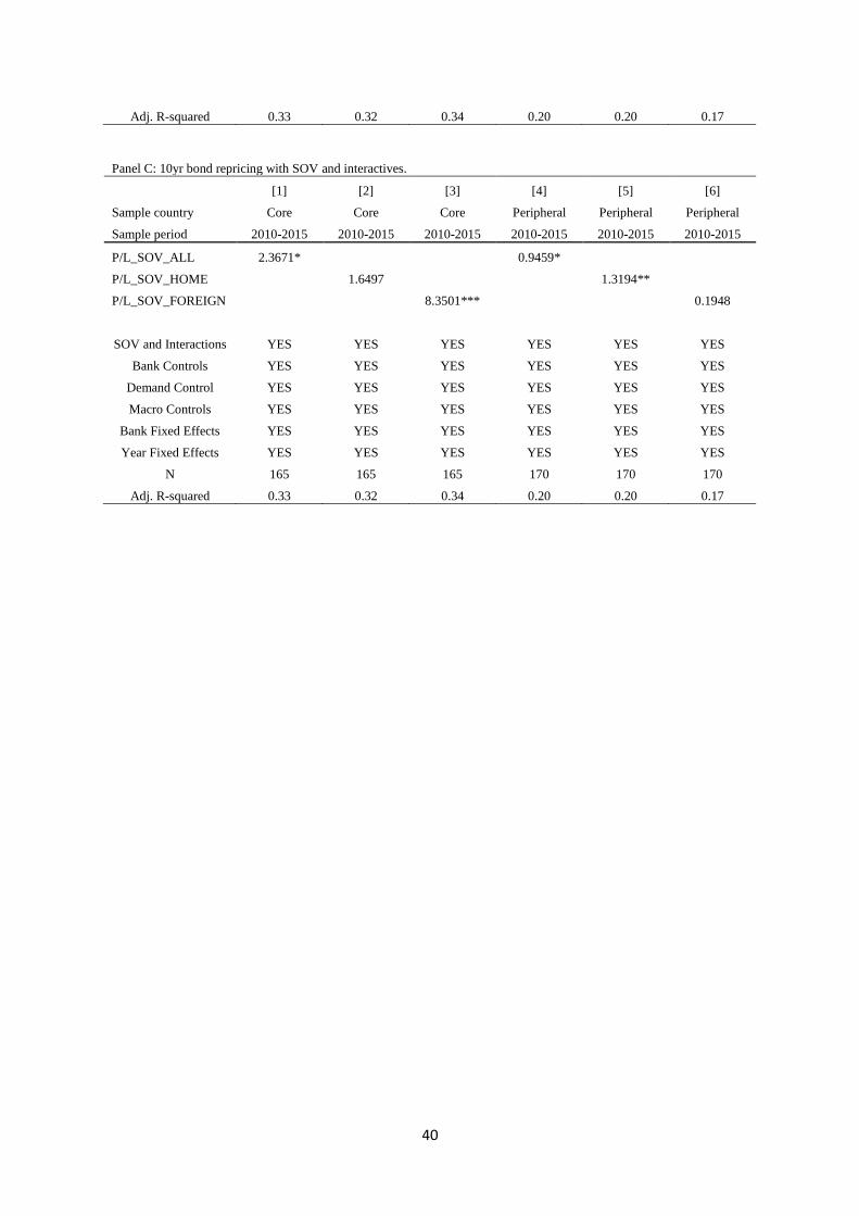
40

Adj. R-squared 0.33 0.32 0.34 0.20 0.20 0.17

Panel C: 10yr bond repricing with SOV and interactives.

[1] [2] [3] [4] [5] [6]


Sample period 2010-2015 2010-2015 2010-2015 2010-2015 2010-2015 2010-2015

P/L_SOV_ALL 2.3671* 0.9459*

P/L_SOV_HOME 1.6497 1.3194**

P/L_SOV_FOREIGN 8.3501*** 0.1948

SOV and Interactions YES YES YES YES YES YES






N 165 165 165 170 170 170

Adj. R-squared 0.33 0.32 0.34 0.20 0.20 0.17

41

Appendix A: Bank Lending Survey and Demand Index

Based on the bank lending survey conducted by the ECB since 2003, we could have some

ideas about the demand and supply changes over time. The survey is addressed to senior loan

officers of a representative sample of euro area banks and is conducted four times a year. The

sample group participating in the survey comprises around 140 banks from all euro area

countries and takes into account the characteristics of their respective national banking

structures.

We are particularly interested in the results of a few survey questions – Q1, Q6, Q10 and

Q18, which ask banks how the demand of loan or their supply standard have been changed

regarding the borrowers from different sectors. The responses to such a question are analysed

in this report by focusing on the difference (“net percentage”) between the share of banks

reporting that credit standards have been tightened and the share of banks reporting that they

have been eased. A positive net percentage indicates that a larger proportion of banks have

eased credit standards (“net easing”), whereas a negative net percentage indicates that a larger

proportion of banks has tightened credit standards (“net tightening”). Likewise, the term “net

demand” refers to the difference between the share of banks reporting an increase in loan

demand and the share of banks reporting a decline. Net demand will therefore be positive if a

larger proportion of banks have reported an increase in loan demand, whereas negative net

demand indicates that a larger proportion of banks have reported a decline in loan demand.

Also, the results of the survey are aggregated and reported on a country level basis each quarter.

Apart from “net percentage” there is another measurement called “diffusion index” which

basically is a weighted “net percentage”. Specifically, it gives a weight of 2 for considerably

changed states while a weight of 1 for somewhat changed states. Based on the survey results,

we build an index – DEMD as a country level control variable for demand of loans. Firstly, we

get the diffusion index of the survey corresponding to the demand changes of three sectors,

42

enterprises, house purchases and consumer credit. Notably, based on ECB, the sum of these

three sectors covers all loans to the non-public sector excluding monetary financial institutions

(MFI). Then, we calculate weighted average based on the outstanding amount of loans to each

sector. Lastly, we sum up the weighted index of a year to convert the data from quarter to

annual. Actually, for the DEMD of year t+1, we sum up Q4 of year t and Q1 Q2 and Q3of year

t+1 because all country level macro variables are lagged by 1 quarter. Similarly, we also built

SUPPLY – an index of how bank’s credit supply standard has been changed across different

Eurozone countries.

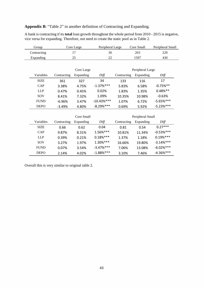
43

Appendix B: “Table 2” in another definition of Contracting and Expanding.

A bank is contracting if its total loan growth throughout the whole period from 2010 - 2015 is negative,

vice versa for expanding. Therefore, not need to create the static pool as in Table 2.

Group Core Large Peripheral Large Core Small Peripheral Small

Contracting 17 30 203 229

Expanding 25 22 1597 430

Core Large Peripheral Large

Variables Contracting Expanding Diff Contracting Expanding Diff

SIZE 361 327 34 133 116 17

CAP 3.38% 4.75% -1.37%*** 5.83% 6.58% -0.75%**

LLP 0.47% 0.45% 0.02% 1.83% 1.35% 0.48%**

SOV 8.41% 7.32% 1.09% 10.35% 10.98% -0.63%

FUND -6.96% 3.47% -10.43%*** 1.07% 6.72% -5.65%***

DEPO -3.49% 4.80% -8.29%*** 0.69% 5.92% -5.23%***

Core Small Peripheral Small

Variables Contracting Expanding Diff Contracting Expanding Diff

SIZE 0.66 0.62 0.04 0.81 0.54 0.27***

CAP 9.87% 8.31% 1.56%*** 10.81% 11.34% -0.53%***

LLP 0.39% 0.21% 0.18%*** 1.37% 1.18% 0.19%***

SOV 3.27% 1.97% 1.30%*** 16.66% 19.80% -3.14%***

FUND 0.07% 3.54% -3.47%*** 7.06% 13.08% -6.02%***

DEPO 2.14% 4.02% -1.88%*** 3.10% 7.46% -4.36%***

Overall this is very similar to original table 2.

44

Appendix C: Bankscope vs. EBA, large banks 2010-2015.

The purpose of this table is to compare the results between EBA and Bankscope data for sovereign exposure information. A

bank is qualified as a large bank if it has participated in the EBA serial tests at least twice. Peripheral countries are Greece,

Ireland, Italy, Portugal and Spain. Core countries are Austria, Belgium, Germany, France and Netherlands. Apart from loan

growth, there are 5 bank level variables. SIZE: log of total asset (in thousand Euros); CAP: total equity / total asset; LLP: loan

loss provision / total loan; SOV: sovereign securities exposure / total asset. Δln(FUND): growth rate of total retail deposit and

short-term funding. DEMD is a country-level variable which describes the changes of credit demand of domestic borrowers.

Macro Controls include domestic GDP and CPI growth rates. SOV is interacted with a dummy variable Crunch which equals

to 1 if the dependent variable is negative and otherwise 0. For banks in peripheral countries during the Eurozone crisis period

(2010-2015), SOV is also interacted with a dummy variable Crisis which equals to 1 for a peripheral country whose average

10-year bond spreads (with respect to Germany) was above 400 basis points, otherwise 0. For all core countries, Crisis equals

to 1 if there are at least two peripheral counties are “in crisis”. Also, we include the result of Wald-Test, which gives the joint

significance of different linear combinations of betas of SOV, SOV*Crunch, and SOV*Crisis. All explanatory variables are

lagged by 1 year. We match the exactly bank-year observation between the two data source and due to limited sample size

bank level variables are winsorized at 10% and 90% for each year within the bank group. Standard errors are heteroscedasticity-

robust and clustered at the bank level. ***, **, and * indicate significance at the 1, 5 and 10 percent levels, respectively.

[1] [2] [3] [4] [5] [6] [7] [8]

Sample Country Core Core Peripheral Peripheral Core Core Peripheral Peripheral

Sample Period 2010-2015 2010-2015 2010-2015 2010-2015 2010-2015 2010-2015 2010-2015 2010-2015

Source for sovereign exposure

Bankscope EBA Bankscope EBA Bankscope EBA Bankscope EBA

SOV_ALLt-1 0.6845* 0.8307** 0.3577** 0.5176*** 0.4635 0.7652** 0.3388** 0.4820**

SOV_ALLt-

1*Crunch -0.6228*** -0.7437*** -0.6198*** -0.7432*** -0.6215*** -0.7595*** -0.6166*** -0.7381***

SOV_ALLt-1*Crisis 0.4238 0.5438 0.052 0.092

Δln(loan)t-1 -0.1378 -0.1281 -0.0071 0.0287 -0.1546* -0.108 -0.0054 0.0309

SIZEt-1 -0.0449*** -0.0465* -0.0697** -0.0631*** -0.0540*** -0.0506* -0.0687** -0.0623***

CAPt-1 2.0009*** 2.1253*** 0.1926 -0.0131 2.0378*** 2.1551*** 0.1608 -0.0424

LLPt-1 5.3911* 5.3293* -0.2804 -0.542 4.8079 5.7209** -0.2395 -0.5145

Δln(FUND)t-1 -0.0584** -0.0441 -0.0877* -0.1030* -0.0421 -0.0397 -0.0886* -0.1050*

DEMDt-1 -0.0001 0.001 -0.0001 -0.0002 -0.0001 0.001 -0.0001 -0.0002

Macro Controls YES YES YES YES YES YES YES YES

Bank Fixed Effects

YES YES YES YES YES YES YES YES

Year Fixed Effects

YES YES YES YES YES YES YES YES

N 116 116 163 163 116 116 163 163

Adj. R-Squared 0.66 0.62 0.58 0.53 0.67 0.63 0.58 0.53

Wald test

SOV 0.6845* 0.8307* 0.3577** 0.5176*** 0.4635 0.7652** 0.3388** 0.4820**

SOV*(1+Crunch) 0.06170 0.0870 -0.2621** -0.2256* -0.1580 0.0057 -0.2778** -0.2561*

SOV*(1+Crisis) 0.8873* 1.3090** 0.3908** 0.5740***

SOV*(1+Crunch+Crisis)

0.2658 0.5495 -0.2258 -0.1641

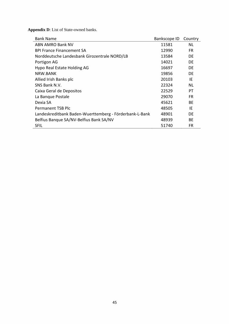
45

Appendix D: List of State-owned banks.

Bank Name Bankscope ID Country

ABN AMRO Bank NV 11581 NL

BPI France Financement SA 12990 FR

Norddeutsche Landesbank Girozentrale NORD/LB 13584 DE

Portigon AG 14021 DE

Hypo Real Estate Holding AG 16697 DE

NRW.BANK 19856 DE

Allied Irish Banks plc 20103 IE

SNS Bank N.V. 22324 NL

Caixa Geral de Depositos 22529 PT

La Banque Postale 29070 FR

Dexia SA 45621 BE

Permanent TSB Plc 48505 IE

Landeskreditbank Baden-Wuerttemberg - Förderbank-L-Bank 48901 DE

Belfius Banque SA/NV-Belfius Bank SA/NV 48939 BE

SFIL 51740 FR

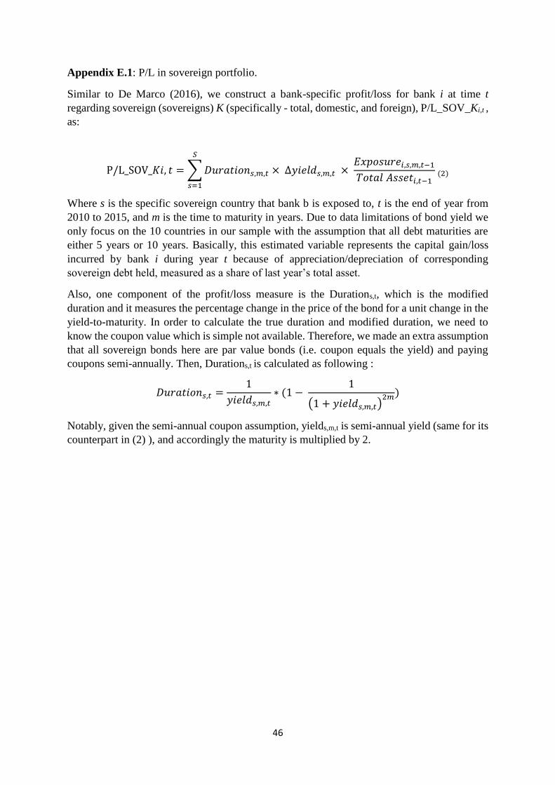
46

Appendix E.1: P/L in sovereign portfolio.

Similar to De Marco (2016), we construct a bank-specific profit/loss for bank i at time t

regarding sovereign (sovereigns) K (specifically - total, domestic, and foreign), P/L_SOV_Ki,t ,

as:

P/L_SOV_𝐾𝑖, 𝑡 = ∑ 𝐷𝑢𝑟𝑎𝑡𝑖𝑜𝑛𝑠,𝑚,𝑡 × ∆𝑦𝑖𝑒𝑙𝑑𝑠,𝑚,𝑡 × 𝐸𝑥𝑝𝑜𝑠𝑢𝑟𝑒𝑖,𝑠,𝑚,𝑡−1

𝑇𝑜𝑡𝑎𝑙 𝐴𝑠𝑠𝑒𝑡𝑖,𝑡−1

𝑆

𝑠=1

(2)

Where s is the specific sovereign country that bank b is exposed to, t is the end of year from

2010 to 2015, and m is the time to maturity in years. Due to data limitations of bond yield we

only focus on the 10 countries in our sample with the assumption that all debt maturities are

either 5 years or 10 years. Basically, this estimated variable represents the capital gain/loss

incurred by bank i during year t because of appreciation/depreciation of corresponding

sovereign debt held, measured as a share of last year’s total asset.

Also, one component of the profit/loss measure is the Durations,t, which is the modified

duration and it measures the percentage change in the price of the bond for a unit change in the

yield-to-maturity. In order to calculate the true duration and modified duration, we need to

know the coupon value which is simple not available. Therefore, we made an extra assumption

that all sovereign bonds here are par value bonds (i.e. coupon equals the yield) and paying

coupons semi-annually. Then, Durations,t is calculated as following :

𝐷𝑢𝑟𝑎𝑡𝑖𝑜𝑛𝑠,𝑡 =1

𝑦𝑖𝑒𝑙𝑑𝑠,𝑚,𝑡∗ (1 −

1

(1 + 𝑦𝑖𝑒𝑙𝑑𝑠,𝑚,𝑡)2𝑚)

Notably, given the semi-annual coupon assumption, yields,m,t is semi-annual yield (same for its

counterpart in (2) ), and accordingly the maturity is multiplied by 2.

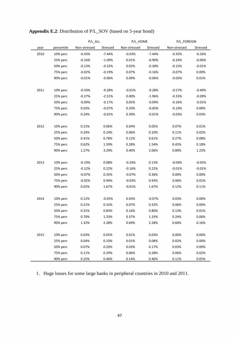
47

Appendix E.2: Distribution of P/L_SOV (based on 5-year bond)

P/L_ALL P/L_HOME P/L_FOREIGN

year percentile Non-stressed Stressed Non-stressed Stressed Non-stressed Stressed

2010 10% perc -0.43% -7.44% -0.03% -7.44% -0.35% -0.26%

25% perc -0.16% -1.09% 0.01% -0.90% -0.24% -0.06%

50% perc -0.13% -0.32% 0.02% -0.30% -0.15% -0.01%

75% perc -0.02% -0.19% 0.07% -0.16% -0.07% 0.00%

90% perc -0.01% -0.06% 0.09% -0.06% -0.03% 0.01%

2011 10% perc -0.50% -9.28% -0.01% -9.28% -0.57% -0.49%

25% perc -0.27% -2.51% 0.00% -1.96% -0.33% -0.09%

50% perc -0.09% -0.17% 0.05% -0.09% -0.16% -0.01%

75% perc 0.03% -0.07% 0.20% -0.05% -0.10% 0.00%

90% perc 0.24% -0.01% 0.39% -0.01% -0.03% 0.03%

2012 10% perc 0.15% 0.06% 0.04% 0.05% 0.07% 0.01%

25% perc 0.24% 0.24% 0.06% 0.10% 0.11% 0.02%

50% perc 0.41% 0.78% 0.12% 0.61% 0.27% 0.08%

75% perc 0.62% 1.59% 0.28% 1.54% 0.45% 0.18%

90% perc 1.27% 3.29% 0.40% 2.06% 0.89% 1.23%

2013 10% perc -0.19% 0.08% -0.24% 0.13% -0.04% -0.05%

25% perc -0.12% 0.22% -0.16% 0.22% -0.01% -0.01%

50% perc -0.07% 0.35% -0.07% 0.36% 0.00% 0.00%

75% perc -0.02% 0.94% -0.03% 0.93% 0.06% 0.01%

90% perc 0.02% 1.67% -0.01% 1.67% 0.12% 0.11%

2014 10% perc 0.12% -0.05% 0.03% -0.07% 0.03% 0.00%

25% perc 0.21% 0.32% 0.07% 0.32% 0.06% 0.00%

50% perc 0.31% 0.83% 0.16% 0.80% 0.13% 0.01%

75% perc 0.70% 1.33% 0.37% 1.33% 0.24% 0.06%

90% perc 1.32% 2.28% 0.69% 2.28% 0.60% 0.16%

2015 10% perc 0.03% 0.05% 0.01% 0.03% 0.00% 0.00%

25% perc 0.04% 0.10% 0.01% 0.08% 0.02% 0.00%

50% perc 0.07% 0.20% 0.03% 0.17% 0.03% 0.00%

75% perc 0.11% 0.29% 0.06% 0.28% 0.06% 0.02%

90% perc 0.25% 0.46% 0.14% 0.46% 0.11% 0.05%

1. Huge losses for some large banks in peripheral countries in 2010 and 2011.

sovereign debt and bank loans: complements or substitutes?

Documents