financial subsidies and bank lending: substitutes or ... subsidies and bank lending: substitutes or...

Financial subsidies and bank lending: substitutes or

complements? Micro level evidence from Italy

Amanda Carmignani∗and Alessio D’Ignazio†

Bank of Italy

December 2010

Abstract

We exploit Italian Central Credit Register data to investigate theeffectiveness of subsidized credit programs for public financing to firmsvia the banking system. The effect of public incentives depends on theavailability of financial resources for the beneficiary firms. Financiallyconstrained firms are likely to use the subsidies to expand output, whileless constrained firms will, at least partly, use the funds to replace morecostly resources. Focusing on the relationship between bank credit andsubsidized loans, we find that larger firms substitute public financingfor bank lending, while there is not such evidence for smaller firms.The estimated degree of substitution is substantial, ranging from anestimated 70 per cent to 84 per cent.

JEL classification: G2, H2, O16

Keywords: Financial subsidies, Credit constraints, Banking

We thank Antonio Accetturo, Raffaello Bronzini, Luigi Cannari, Guido de Blasio,Francesca Lotti, Guido Pellegrini, Alberto Pozzolo, Mario Quagliariello, Enrico Rettore,Paolo Sestito, two anonymous referees and participants at the Bank of Italy’s seminar onpublic incentives for firms (Rome, April 2010) and at the DIME International Workshopon Financial Constraints, Firm and Aggregate Dynamics (Sophia-Antipolis, December2010) for valuable comments and suggestions. The usual disclaimer applies. The viewsexpressed herein are those of the authors and do not necessarily reflect those of the Bankof Italy.∗Research Department, Bank of Italy, Via Nazionale 91, 00184 Roma, Italy. Email

address: [email protected].†Research Department, Bank of Italy, Via Nazionale 91, 00184 Roma, Italy. Email

address: [email protected].

1 Introduction

Many governments have programs to support the productive system, inparticular small and medium-sized enterprises (SMEs). They consist largelyof financial subsidies designed to reduce market failures, mainly financialconstraints on SMEs. The European Commission has increased the leewayfor State aid, especially to SMEs (European Commission, 2009). Subsidiesto SMEs represent about 10 per cent of the total amount of state aid inthe EU27. In Italy, where the productive system consists almost entirely ofSMEs, the share was 37 per cent in 2007.

In view of the widespread use of these policies in the EU, and partic-ularly in Italy, this paper analyzes the effectiveness of subsidized credit inalleviating financial constraints and hence promoting growth1.

We focus on subsidized credit programs for public financing to firms viathe banking system. The effect of public incentives is related to the availabil-ity of financial resources for the beneficiary firms. Financially unconstrainedfirms will presumably use public resources to substitute, at least partly, formore costly private credit, while firms with less access to external financingwill use the subsidies to expand investment and output. To evaluate theeffectiveness of subsidized lending we test the relationship of complemen-tarity/substitutability between bank credit and public financing in a set ofItalian firms that benefited from subsidized credit programs.

Both the theoretical and the empirical literature have studied the issue offirms’ financial constraints on firms (for a review see Hubbard (1998), Bondand Van Reenen (2007)), although this work has suffered from paucity ofdata and methodological problems. Fazzari, Hubbard and Petersen (1988)investigate the effects on investment of the availability of close substitutesfor credit, using the sensitivity of investments to cash flow as a measureof financial constraints. This approach has been challenged by Kaplan andZingales (1997), who observed that this gauge might reflect endogeneityproblems, since both investment and cash flow depend on profitability. Inorder to test for this causality, a large body of research has examined thedifferences in the investment-cash flow correlation between groups of firmsthat are reasonably expected to face different financial constraints. For themost part the results support Fazzari et al. (1988)2.

In a related stream of literature, Banerjee and Duflo (2008) test for theexistence of credit constraints by exploiting variations in policy measures

1Among the research papers indicating a relationship between internal finance andsmall firms growth see Carpenter and Petersen (2002).

2Whited (1992) provides empirical evidence supporting the dependence of some firms’investment on liquidity variables; Shaller (1993) finds that investment is far less liquidity-constrained for firms with less costly access to equity financing; Bond and Meghir (1994)use UK data and find that current investment positively depends on lagged cash flow. SeeBond and Van Reenen (2007) for a survey.

2

involving the supply of directed credit in India. Zia (2008) identifies creditconstraints by exploiting a change in eligibility criteria for subsidized loansand comparing outcomes before and after the policy change. Lamont (1997)exploits the 1986 oil price shock to find an exogenous instrument for cash,showing that a decrease in cash flow leads to a fall in investment. ForItaly, similar issues are investigated by Albareto, Bronzini, de Blasio andRassu (2008) with regard to public grants channelled to companies througha specific incentive scheme aimed at promoting investment (Law 488/92).

The empirical literature mainly focuses on larger firms, owing to dataavailability. In this paper we fill the gap by exploiting a unique datasetthat has bank-firm information on small and micro enterprises from 1998 to2007, drawn from the Central Credit Register database. Using a programevaluation approach, we compare the proportional change in the amount ofbank credit used by firms before and after the policy intervention. Whileboth “more constrained” and “less constrained” firms seek subsidized lend-ing, since it is cheaper, the latter will mainly use it to substitute for bankcredit.

Our analysis shows that subsidized loans are used as substitutes for banklending by the larger firms, but not by partnerships and small firms. Overall,the degree of substitution between public resources and bank lending issubstantial, ranging from about 70 to 84 per cent. While this evidencesupports the thesis that small firms are at a disadvantage in attractingfinancing (Berger and Udell, 2002) it also suggests a significant misallocationof public resources: only a small part of the funds is allocated to trulyconstrained firms (small firms). Our results are robust to a broader notionof treatment, alternative model specifications and the introduction of firms’balance-sheet data.

The remainder of the paper is structured as follows. In section 2 weprovide some information on the system of firm subsidies in Italy and ourdataset, while section 3 describes the rationale behind our evaluation ex-ercise and illustrate the empirical strategy. The main results are given insection 4, robustness checks in sections 5 and 6. Section 7 concludes.

2 Firm subsidies and the Central Credit Register

State aid to the productive system includes the following measures: grants,subsidized loans, tax relief and tax credits, state guarantees and holdings.Grants and subsidized loans have been extensively used in Italy. In the caseof grants, the subsidy takes the form of a lump sum, which is proportionaleither to the amount of the investment or to the costs borne by the firm.In the case of subsidized loans, the incentive can be either a transfer aimedat reducing the interest rate of an underlying bank loan, or a public loangranted at a lower-than-market interest rate.

3

In this paper we focus on the latter type of subsidy, where the State(both central and local governments) disburses the loan, and we will refer toit interchangeably as subsidized lending, public loans or subsidized credit.These incentives essentially involve medium and long term financing andrepresent the main type of subsidy employed in the Centre and North ofItaly. On the other hand, grants have been historically employed in theSouth of the country, since the launch in 1951 of the “Fund for the South”program (Cassa per il Mezzogiorno). The initiative had been set up to at-tract private investment in Southern Italy but turned out to be unsuccessfuland was ended in 19923. It was replaced by a program based on a similardesign (the so called Law 488) which shared the same destiny (Bronzini andde Blasio (2006)). After the failure of the policies based on grants, Italianpolicy makers have focused on public loans to sustain the productive system.As present, little is known about the effectiveness of these measures.

State aid to firms in Italy is provided by means of a series of programs,which are managed by central, regional and local governments. Aggregatedata on firm aids are provided by the Ministry of Economic Development,while micro level data are available only for a very small set of measures.By exploiting the Central Credit Register (CCR) held at the Bank of Italy,in this paper we employ a unique dataset consisting of micro-level dataon a wide set of subsidized lending programs. Private banks, in fact, actas State agents for this type of subsidies and perform both the selection ofapplicants and the management of the public loans. According to the ItalianBanking Regulation “for each borrower, financial intermediaries supervisedby the Bank of Italy have to report to the CCR, on a monthly basis, theamount of each loan, either granted or disbursed by banks, for all loansexceeding a given threshold” (the threshold was e 75,000 until 31 December20084). Banks report to the CCR also the information on loans provided onbehalf of central and local governments(“third party account operations”;see Caprara, Carmignani and D’Ignazio (2009) for a detailed description ofthe data used in this work).

Our dataset refers to the period 1998-2007 and contains information onmore than 200 intermediaries acting as State agents and more than 20,000firms. In 2007 the amount of public loans reported in the CCR reachedabout e4.7 billion, representing about 12 per cent of total state aid to firms(which includes also grants, financial guarantees and lump sum transfers).If we focus only on measures involving, at least in part, a public loan, theshare rises up to 30 per cent.

Regions in the North of the country and the autonomous regions with3The funds channeled through the Fund for the South over the period 1951-1992

amounted to about e140,000,000.4In January 2009 the threshold was lowered to e 30,000. Bad loans continue to be

reported to the CCR regardless of the amount.

4

Figure 1: Public loans over Regional GDP (left panel) and share of beneficiary firmsover total firms (right panel) in 2007

a special statute5 have received the largest share of public loans. In 2007about 36 per cent of the funding attained firms located in the regions withspecial statute. Figure 1 shows that these regions but one are in the highestquartile of the distribution in terms of both financial resources received andnumber of firms benefited. As for the funding, about 80 per cent of theresources are allocated to large firms, which represent about 50 per cent ofthe beneficiaries.

The public loans that we observe relate to a wide array of national andregional programs mostly aimed at boosting investments and easing accessto credit. In particular, a large set of these measures indicate the aim toease firms’ access to credit6, while the majority of the programs specify theinvestment target. Public loans are granted on favorable terms (the interestrate is lower-than-the market interest rate) and are provided to firms inone or more installments by the state agent bank. Firms reimburse theloans over a period of about 7-10 years; the repayment usually starts after a“grace period” (not exceeding two years). Banks screen the applicants on the

5The Italian state is administratively divided into twenty regions. Among them five re-gions are constitutionally given a broader amount of autonomy granted by special statutes(namely, Valle d’Aosta, Trentino-Alto Adige, Friuli-Venezia Giulia, Sicily and Sardinia).

6See regional law 18/99 and regional law 27/00 in Piedmont; regional law 27/06 inLazio; regional law 1/99 in Veneto; regional law n. 34/96 in Lombardy; measure 2.1 ofthe regional law 1997/99 for Ferrara; and Seed capital fund in Reggio Calabria.

5

basis of the requirements of the law underlying the subsidy (such conditionsmostly involve firm size, geographical location, sector of economic activityand investment plan) and, in some cases, provide a screening of the firmreimbursement capacity.

3 Theoretical background and empirical strategy

Following the seminal paper of Fazzari et al. (1988) (hereinafter FHP), alarge body of research focussed on the role of capital market frictions andfirm access to external finance in determining investments. In their depar-ture from the keynesian assumption that all firms respond similarly to thecost of capital, FHP introduced a model of financing hierarchy, where in-ternal finance has cost advantages over external funds. In the FHP model,firms have different abilities to raise funds externally, depending on infor-mation asymmetries. Firms subject to stricter constraints in raising fundsexternally have greater investment-cash flow sensitivity, so for them the in-vestment response to an increase in internal funds is greater.

Figure 2 shows the case of two firms with the same technology (repre-sented by the marginal revenue curve, MRK) and amount of internal funds(k0), but facing different levels of financial constraints (high or low). Theconstraint is represented by the steepness of the upward-sloping part of thefund supply curve (represented by the marginal costs, SH and SL, respec-tively). Let k0 be the amount of the firm internal funds, and kH and kL theinitial equilibrium levels of capital for the more constrained (type-H) andthe less constrained (type-L) firm, respectively. After a windfall increase ininternal funds ∆s is introduced, the fund supply curve for both firms shiftsto the right. A positive effect on investment will follow. The effect will begreater for the more severely constrained firm. In the extreme case of totalcredit rationing (vertical fund supply curve), the new funds will translatefully into additional capital. On the other hand, in the case of perfect capitalmarkets (flat supply curve), they will entirely crowd out more costly credit.

In the hierarchy-of-finance framework, the introduction of subsidizedcredit (at an interest rate lower than r0) is equivalent to a windfall in-crease in internal funds. The FHP model then predicts that subsidies willbe more effective if they go to financially constrained firms. Less financiallyconstrained firms, on the other hand, will use the subsidy to replace morecostly credit, the degree of substitution being inversely proportional to theseverity of the financial constraints.

This framework relies on two key assumptions: the cost of external fundsto the firm does not fall when the firm gets the subsidy; firms technologymust not change with the subsidy. According to the literature, firm size isa proxy for transparency of enterprises (Berger and Udell, 2002): the largerthe firm, the smaller the informational gap and the greater the ability to

6

rMRK

k

SH S′H

SL

S′Lr0

∆s

k0 k′0 kH k

′H kL k

′L

Figure 2: The impact of a windfall increase in internal funds on investments

raise external funds. Hence, we expect that larger firms will be marked bygreater substitutability between subsidized credit and bank loans.

Our dataset refers to the period 1998-2007 and contains informationon sector of economic activity, legal form, location, amount of credit bothgranted and disbursed by banks, and for the beneficiary firms the amount ofsubsidized loans. We compare the dynamics of subsidized credit with thatof medium and long term bank loans7.

Building on the rationale presented before, we devise a test to estimatethe extent to which public resources actually reach truly credit-constrainedenterprises. Our dependent variable is recourse to bank credit8; however,since the amount of credit used is strongly auto-correlated, we consider itsproportional change (see Banerjee and Duflo (2008)).Ideally, in order to identify the causal effect of the policy we should com-pare firms’ recourse to bank credit in the presence of the treatment (gettingthe subsidy) with the recourse to bank credit in the case of no treatment.Evidence of substantial substitutability would indicate that the program’seffect was limited. However, for subsidized firms we can only observe theoutcome under the program (factual outcome; see Holland (1986)). To over-come this problem we consider average causal effects by comparing distinctunits exposed and not exposed to the program. These units can be eitherdifferent physical units or the same unit at different times.

7In an unreported exercise we perform our analysis by considering total bank loans,obtaining very similar results. The subsidized loans represent, on average, slightly lessthan 10 per cent of total bank loans for the entire set of beneficiary firms.

8According to Cerved archive, which groups balance sheet data on all Italian limitedcompanies from 1993 onwards, in 2007 bank debt represents almost 80 per cent of mediumand small firms’ financial debt.

7

We exploit the longitudinal nature of our dataset to estimate the causaleffect. Let Y be the outcome variable we are interested in, D a dummyequal to 1 for treated firms and 0 for untreated. Let us assume that thetreatment is carried out in a time period between τ and t. We are interestedin estimating the average treatment effect on the treated (ATT ). If inthe absence of treatment the difference between the groups of treated anduntreated firms is constant over time, the ATT is correctly estimated by thefollowing difference-in-differences (DID) model, following Ashenfelter andCard (1985):

Yi = β0 + β1Di + β2POST + δDiPOST + εi,t (1)

where Yi is the outcome variable and POST is a dummy assuming value 1in the treatment years. The estimated parameter of interest is δ̂.

“Treated” firms are those receiving subsidies. Although the financialsubsidies are provided under different laws, the dataset has no informationto distinguish among them. The subsidized loans differ in disbursement andreimbursement schemes. In some cases, firms start repayment the next year;in most, after a two year “grace period”. In order to have an homogeneousform of treatment, we take only the latter scheme and thus consider a three-year treatment period window: the year of the first disbursement followedby a two-year grace period, where the amount of subsidies enjoyed by thebeneficiary firms is non-decreasing.

Figure 3: Sampling groups

The the pre-intervention window considered is also three years. Hence,our first group of treated subjects consists of firms that were not subsidizedin the period 1998-2000 and that received their first subsidy in 2001. We end

8

up with five groups of “treated” firms, one for each possible “first year oftreatment” between 2001 and 2005. Figure 3 shows the groups, with t beingthe first year of treatment. The dataset we end up with is a rotating panel,with five groups of firms in the sample for a period of six consecutive years,centered on the first year of treatment. The total number of beneficiariesis almost 400. The set of untreated firms comprises all the firms that havenever received a public credit subsidy in the Credit register.

The main challenge for our analysis is constructing a valid control group.In assessing firms’ elegibility for the incentives, the intermediaries acting asstate agents take into account both firm characteristics and credit history.On this basis, we use the information contained in the CCR dataset toperform a one-to-one exact matching procedure. Given our rotating dataset,we consider one group of treated at a time. For each, in the first step weassociate to each treated firm all the untreated firms characterized by thesame sector, location and legal form. To avoid the general equilibrium effectsthat could arise when both treated and untreated firms are selected fromthe same local area (Busso and Kline (2008)), we match firms using regionalrather than provincial boundaries.

To take account of the firm’s loan pre-treatment dynamics, we also per-form a match on the class of debt (credit used) over the years (t-3), (t-2)and (t-1), where t is the first year of treatment. We also consider theamount granted in the pre-intervention period. For each of the five groupsof matched units, we define the first year of treatment as year t, and aggre-gate the samples to obtain a single dataset. Besides firms’ characteristics,for which we performed exact matching, the control group exactly mirrorsthe set of treated firms also with regard to the distribution of debt growthrates in the pre-treatment period (see figure 4).

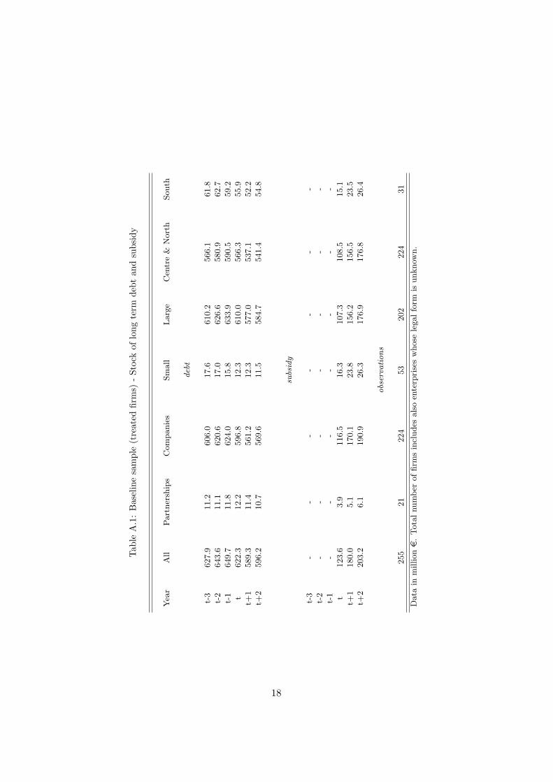
After performing the exact matching and trimming both the set oftreated and untreated firms at the 5th and 95th percentile of debt growthrates, our dataset consists of 255 treated and 255 untreated firms9. Theyare mostly limited companies, firms headquartered in the Centre and North,and firms whose average debt is more than e 500,000 (labeled as “large”firms). Table A.1 and table A.3 show respectively the yearly evolution inthe stock of both bank debt and subsidy and the average amount of debtfor both treated and untreated firms.

4 Baseline results

Table 1 shows the average bank debt before and after the policy interven-tion for both treated and untreated firms. By construction, the differencebetween treated and untreated firms is small in the pre-treatment period;

9Having an equal sample size for both treated firms and controls increases the powerto detect a difference between the two groups.

9

Figure 4: Kernel density, debt in the pre-treatment years for treated and untreatedfirms

in the post-intervention period, treated firms have less bank debt.To study the relationship between public subsidies and bank credit, we

estimate the following difference-in-differences (DID) model:

yi = β0 + β1dsubsidyi + β2post+ δdsubsidyi · post+ εi,t (2)

where yi is the rate of growth of the debt, “dsubsidy” is a dummy indicatingwhether or not the firm received the public loan, and “post” is a dummyequal to 1 from time t onwards. If the model’s assumptions hold, the DIDcorrectly estimates δ̂, measuring how much the firms actually getting thesubsidies changed their recourse to bank credit.

Table A.5 reports the estimates of the DID model. On average, firms douse subsidized credit mostly as a substitute for market credit. The effect,however, varies with firms’ characteristics, being marked for large firms andcompanies, trivial for smaller firms (those with average private debt belowe500,000) and partnerships. Using the median in firms’ debt distribution toidentify large and small firms could represent a source of potential bias. Tocontrol for this issue, we refined our strategy dropping from the sample allfirms with a debt level close to the median in the pre-treatment years. Theresults obtained on the smaller sample (not reported) confirm the findings inthe baseline model. Moreover, the results vary with the geographical area,the substitution effect characterizing essentially the Centre and the North ofthe country (see table A.5). However, we interpret the results for the Southcautiously since the number of observations available for that area is verysmall.

To control for the possibility that our results suffer from anticipation

10

Table 1: Debt toward banks for treated and untreated firms(Baseline sample; million e)

pre treatment years average post treatment years average

treated firms 640.4 602.6untreated firms 644.6 661.0

effects, which might influence private debt dynamics in the year immedi-ately preceding the treatment, we re-estimated the DID model consideringa long pre-intervention window (five years). The results (not reported) arevery similar to those in the baseline. Finally, taking into account that inthe period under consideration securitization played a crucial role in theeconomy, we performed a robustness check by removing from the sample allfirms involved in securitization operations (about 2 percent of the sample);the results did not change.

4.1 Degree of substitution

In order to assess the significance of our results we need to measure themagnitude of the substitution effect between private and public loans. Tocalculate the degree of substitution (ds) we use the estimated δ and theaverage level of debt in the pre-treatment period:

ds =debtpre(1 + geT ) − debtpre(1 + gcT )∑t+2

t subsidyt

(3)

where T is the number of years of treatment; debtpre is the average amountof debt in the pre-treatment period; ge is the actual average growth rate ofbank credit after the subsidy, gc is the counterfactual (unobservable) growthrate of bank credit that would have occurred had there been no treatment;subsidyt is the amount of subsidies in year t.

Since δ̂ = ge − gc, we can estimate the degree of substitution, which forthe entire sample appears to be substantial: on average it is about 74 percent. To check for robustness, we performed the same DID analysis for threesubsamples of firms, selected according to the amount of subsidized creditin proportion to bank debt. In subsample 1 the share is from 10 per cent to75 per cent; in subsample 2, between 10 and 100 per cent; in subsample 3,from 10 per cent to 200 per cent. As table A.6 shows, the results obtainedwith the subsamples are quite similar to those for the entire sample. Table2 summarizes the estimated degree of substitution for the four samples oftreated firms.

11

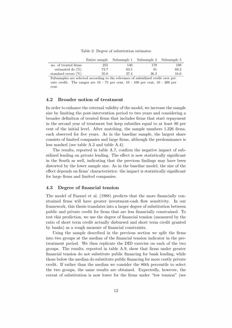
Table 2: Degree of substitution estimates

Entire sample Subsample 1 Subsample 2 Subsample 3

no. of treated firms 255 140 179 199estimated ds (%) 73.7 83.5 81 69.2

standard errors (%) 35.0 37.4 36.3 16.0

Subsamples are selected according to the relevance of subsidized credit over pri-vate credit. The ranges are 10 - 75 per cent, 10 - 100 per cent, 10 - 200 percent.

4.2 Broader notion of treatment

In order to enhance the external validity of the model, we increase the samplesize by limiting the post-intervention period to two years and considering abroader definition of treated firms that includes firms that start repaymentin the second year of treatment but keep subsidies equal to at least 80 percent of the initial level. After matching, the sample numbers 1,326 firms,each observed for five years. As in the baseline sample, the largest shareconsists of limited companies and large firms, although the predominance isless marked (see table A.3 and table A.4).

The results, reported in table A.7, confirm the negative impact of sub-sidized lending on private lending. The effect is now statistically significantin the South as well, indicating that the previous findings may have beendistorted by the lower sample size. As in the baseline model, the size of theeffect depends on firms’ characteristics: the impact is statistically significantfor large firms and limited companies.

4.3 Degree of financial tension

The model of Fazzari et al. (1988) predicts that the more financially con-strained firms will have greater investment-cash flow sensitivity. In ourframework, this thesis translates into a larger degree of substitution betweenpublic and private credit for firms that are less financially constrained. Totest this prediction, we use the degree of financial tension (measured by theratio of short term credit actually disbursed and short term credit grantedby banks) as a rough measure of financial constraints.

Using the sample described in the previous section we split the firmsinto two groups at the median of the financial tension indicator in the pre-treatment period. We then replicate the DID exercise on each of the twogroups. The results, reported in table A.9, show that firms under greaterfinancial tension do not substitute public financing for bank lending, whilethose below the median do substitute public financing for more costly privatecredit. If rather than the median we consider the 80th percentile to selectthe two groups, the same results are obtained. Expectedly, however, theextent of substitution is now lower for the firms under “low tension” (see

12

table A.10).

5 Robustness I

Here we address the potential selection bias arising from our matching pro-cedure. While treated and untreated firms are matched using a set of ob-servable variables that are relevant for firm participation in the programs,other unobservable variables could also be in play, leading to selection bias(a systematic difference between treated firms and control group). Thedifference-in-differences specification is at least a partial solution, as it con-trols for the selection bias resulting from permanent differences between thetreatment and the control group. In this section we attempt to tackle thecase where selection bias is not constant, and estimate the impact of thetreatment by considering only the firms that benefited from the subsidies.In the first exercise we employ a different approach by estimating a dynamicmodel for firm bank credit, while in the second we return to the difference-in-differences methodology.

5.1 GMM approach

In order to assess the impact of subsidized lending on bank credit, we esti-mate the following dynamic model:

debti,t = α1debti,t−1 + α2posti,t + ηi + εi,t (4)

where debti,t is the log of the level of private credit at time t, posti,t is adummy variable assuming value 1 in the years when the firm receives a sub-sidy, and ηi is a firm-time-invariant component. The variable of interestis the dummy post: a negative coefficient would imply a lower recourse tobank credit after the subsidy, thus suggesting substitution between subsi-dized credit and bank loans.

To deal with the potential bias arising from the presence of the laggeddependent variable among the covariates, which would affect a fixed-effectsmodel, we use the general method of moments (GMM) estimator devel-oped by Arellano and Bond (1991). Since firm debt seems to be close toa random walk process (estimations non reported), difference-GMM mightperform poorly. In this case, past levels of a variable are not very goodinstruments for current changes, so we also apply the augmented version ofthe estimator, developed by Blundell and Bond (1998), instrumenting cur-rent levels with past changes. We estimate the models using both a baselinesample, including all firms receiving the treatment (non-decreasing level ofsubsidy) for three years, and an extended sample, including all firms receiv-ing the treatment for at least two years. The results are reported in table

13

A.11 and table A.12. We focus on the Blundell-Bond GMM model(GMM-system) and report, for comparison, the results for the fixed effects and theArellano-Bond GMM (GMM-difference) models.

Overall, the results indicate less debt growth in the post-interventionperiod: the estimated coefficient of the dummy post is negative and statisti-cally significant. This evidence, which is consistent across the three models,supports our previous findings of heterogeneous effects across firms. Thesubsample estimates show that the coefficient of post is statistically signifi-cant only for the set of limited companies and large firms.

5.2 DID on the subsidized firms

To ensure homogeneity between groups, we exploit the features of the incen-tive scheme to select both the treated firms and the control group among thepool of beneficiaries that can be considered similar in terms of all character-istics relevant to obtain the subsidy. To maximize sample size we adopt abroad notion of treatment and a very narrow observation window: the poolconsists of enterprises that one year after the initial disbursement still enjoyat least 80 per cent of the subsidized credit.

We distinguish six groups of beneficiaries on the basis of the first year ofdisbursement (2001 to 2006). The firms that received the subsidy in 2001,2003 and 2005 are considered “treated”; those that received the subsidy in2002, 2004 and 2006 are “controls” (see figure 5). For each group we take afour-year window (t-2, t-1, t and t+1). For the treated the window goes fromtwo years before to the year after the disbursement; for the controls we takethe four years before the disbursement. In this way we end up with 900 firms“treated” and the same number of “controls”. The results, reported in tableA.13, confirm our previous findings: on average, firms substitute cheapersubsidized credit for more expensive private loans. The substitution effectis essentially associated with large firms and limited companies.

6 Robustness II

This paper relies upon the hypothesis that the extent to which subsidizedcredit is used to expand output and investment depends on the severity offirms’ financial constraints. We check this assumption with an evaluationexercise based on real outcomes (output, investment), using balance-sheetdata.

The information is available for limited companies only, hence this sec-tion excludes partnerships. The results of the baseline specification showthat limited companies use subsidized credit as a substitute for bank loans(see table A.5); therefore, in our theoretical framework, we expect no realeffect of the incentive program for these enterprises.

14

Figure 5: Sampling groups of subsidized firms

We merge our dataset with the Cerved archive, which contains balance-sheet data on all Italian limited companies from 1993 onwards. Again, weuse a DID estimator after having performed a one-to-one matching, nowbased also on balance-sheet information. We carry out exact matching onthe following variables: sector of economic activity, location and legal form.To take account of pre-treatment dynamics, we also perform exact matchingon the class of both fixed capital and assets over the years (t-3) and (t-1),where t is the first year of treatment. Finally, we consider average investmentin the pre-intervention period. Our final dataset contains 120 treated andthe same number of untreated firms.

Since in general the incentive programs aim at enhancing the produc-tive system, we take investment(t)/assets(t0) as the outcome variable andestimate model (2). The results, reported in table A.14, show that overallthe credit subsidy has no effect on investment. To look for heterogeneouseffects across firms we split the sample between small and large companiesat the median of assets in the period. In both sub-samples, the estimatesshow that the policy intervention has no impact on firms’ investment. Thesefindings support the previous results based on credit data.

7 Conclusion

Given the widespread use of state aid to SMEs in Italy, we have analyzedto what extent policies based on subsidized loans are effective. The effectof public incentives is related to the availability of financial resources forthe beneficiary firms. Accordingly, our analysis focused on the complemen-

15

tarity/substitutability of public financing and bank credit. We found thatsubsidized lending is used as substitute for bank loans by large firms andlimited companies, while we did not find such evidence for small firms andpartnerships. The degree of substitution between the two sources of fundingis considerable, ranging from 70 to 84 per cent according to our baseline es-timates. This result indicates that the effect of subsidized lending programsin Italy has been modest. Our findings are robust to a broader notion oftreatment, to alternative model specifications and are also supported byresults of a model based on firm balance sheet information.

References

Albareto, G., Bronzini, R., de Blasio, G. and Rassu, R. (2008). Sussidi einvestimenti: un test sui vincoli finanziari delle imprese, Politica Eco-nomica 24.

Arellano, M. and Bond, S. (1991). Some tests of specification for panel data:Monte carlo evidence and an application to employment equations, TheReview of Economic Studies 58.

Ashenfelter, O. and Card, D. (1985). Using the longitudinal structure ofearnings to estimate the effect of training programs, Review of Eco-nomics and Statistics 67: 648–660.

Banerjee, A. and Duflo, E. (2008). Do firms want to borrow more? test-ing credit constraints using a directed lending program, MIT WorkingPaper 02-25 .

Berger, A. and Udell, G. (2002). Small business credit availability andrelationship lending: The importance of bank organisational structure,Economic Journal 112: 32–53.

Blundell, R. and Bond, S. (1998). Initial conditions and moment restrictionsin dynamic panel data models, Journal of Econometrics 87.

Bond, S. and Meghir, C. (1994). Dynamic investment models and the firm’sfinancial policy, Review of Economic Studies 61: 197–222.

Bond, S. and Van Reenen, J. (2007). Microeconometric Models of Investmentand Employment, Vol. 6(65), in J.J. Heckman and E.E. Leamer (ed.),Handbook of Econometrics, North Holland, London, pp. 4417–4498.

Bronzini, R. and de Blasio, G. (2006). Evaluating the impact of investmentincentives: The case of italys law 488/92, Journal of Urban Economics60: 327–349.

16

Busso, M. and Kline, P. (2008). Do local economic development programswork? evidence from the federal empowerment zone program, YaleUniversity, Cowles Foundation Discussion paper No. 1638 .

Caprara, D., Carmignani, A. and D’Ignazio, A. (2009). Gli incentivi pub-blici alle imprese: evidenza a livello micro, forthcoming, Bank of ItalyOccasional papers .

Carpenter, R. E. and Petersen, B. C. (2002). Is the growth of small firmsconstrained by internal finance?, The Review of Economics and Statis-tics 84: 289–309.

European Commission (2009). Handbook on community state aid rules forsmes, EC Studies and reports .

Fazzari, S., Hubbard, R. and Petersen, B. (1988). Financing constraints andcorporate investment, Brookings Papers on Economic Activity 1: 141–195.

Holland, P. (1986). Statistics and causal inference, Journal of the AmericanStatistical Association 81: 945–970.

Hubbard, R. G. (1998). Capital-Market Imperfections and Investments,Journal of Economic Literature 36(1): 193–225.

Kaplan, S. and Zingales, L. (1997). Do investment-cash flow sensitivitiesprovide useful measures of financing constraints, Quarterly Journal ofEconomics 112: 169–215.

Lamont, O. (1997). Cash flow and investment: Evidence from internalcapital markets, The Journal of Finance 52: 83–109.

Shaller, H. (1993). Asymmetric information, liquidity constraints and cana-dian investment, Canadian Journal of Economics 26: 552–574.

Whited, T. M. (1992). Debt, liquidity constraints and corporate investment:evidence from panel data, Journal of Finance 47: 1425–1460.

Zia, B. H. (2008). Export incentives, financial constraints, and the(mis)allocation of credit: Micro-level evidence from subsidized exportloans, Journal of Financial Economics 87: 498–527.

17

Tab

leA

.1:

Bas

elin

esa

mpl

e(t

reat

edfir

ms)

-St

ock

oflo

ngte

rmde

btan

dsu

bsid

y

Yea

rA

llP

art

ner

ship

sC

om

panie

sSm

all

Larg

eC

entr

e&

Nort

hSouth

deb

t

t-3

627.9

11.2

606.0

17.6

610.2

566.1

61.8

t-2

643.6

11.1

620.6

17.0

626.6

580.9

62.7

t-1

649.7

11.8

624.0

15.8

633.9

590.5

59.2

t622.3

12.2

596.8

12.3

610.0

566.3

55.9

t+1

589.3

11.4

561.2

12.3

577.0

537.1

52.2

t+2

596.2

10.7

569.6

11.5

584.7

541.4

54.8

subs

idy

t-3

--

--

--

-t-

2-

--

--

--

t-1

--

--

--

-t

123.6

3.9

116.5

16.3

107.3

108.5

15.1

t+1

180.0

5.1

170.1

23.8

156.2

156.5

23.5

t+2

203.2

6.1

190.9

26.3

176.9

176.8

26.4

obs

erva

tions

255

21

224

53

202

224

31

Data

inm

illione

.T

ota

lnum

ber

of

firm

sin

cludes

als

oen

terp

rise

sw

hose

legal

form

isunknow

n.

18

Tab

leA

.2:

Ext

ende

dsa

mpl

e(t

reat

edfir

ms)

-St

ock

oflo

ng-t

erm

debt

and

subs

idy

Yea

rA

llP

art

ner

ship

sL

imit

edco

mpanie

sSm

all

Larg

eC

entr

e&

Nort

hSouth

deb

t

t-3

2189.1

152.6

1965.0

146.9

2042.2

2024.8

164.3

t-2

2233.7

160.8

1997.0

144.7

2088.9

2067.0

166.7

t-1

2259.5

160.2

2021.7

138.9

2120.6

2092.3

167.2

t2207.9

156.2

1982.4

133.2

2074.6

2053.8

154.1

t+1

2139.9

142.9

1927.1

122.1

2017.8

1988.9

151.0

subs

idy

t-3

--

--

--

-t-

2-

--

--

--

t-1

--

--

--

-t

454.0

52.0

383.6

90.9

363.1

390.3

63.7

t+1

523.4

50.8

453.4

100.2

423.2

451.9

71.5

obs

erva

tions

1326

382

892

541

785

1189

137

Data

inm

illione

.T

ota

lnum

ber

of

firm

sin

cludes

als

oen

terp

rise

sw

hose

legal

form

isunknow

n.

19

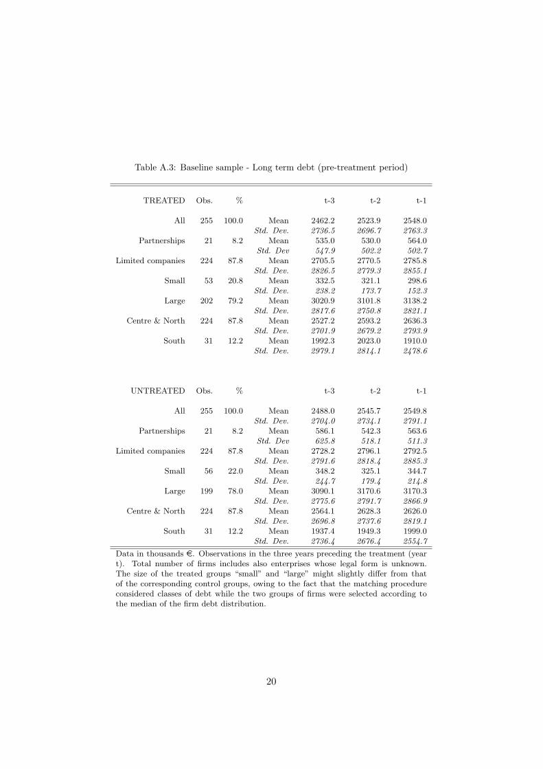
Table A.3: Baseline sample - Long term debt (pre-treatment period)

TREATED Obs. % t-3 t-2 t-1

All 255 100.0 Mean 2462.2 2523.9 2548.0Std. Dev. 2736.5 2696.7 2763.3

Partnerships 21 8.2 Mean 535.0 530.0 564.0Std. Dev 547.9 502.2 502.7

Limited companies 224 87.8 Mean 2705.5 2770.5 2785.8Std. Dev. 2826.5 2779.3 2855.1

Small 53 20.8 Mean 332.5 321.1 298.6Std. Dev. 238.2 173.7 152.3

Large 202 79.2 Mean 3020.9 3101.8 3138.2Std. Dev. 2817.6 2750.8 2821.1

Centre & North 224 87.8 Mean 2527.2 2593.2 2636.3Std. Dev. 2701.9 2679.2 2793.9

South 31 12.2 Mean 1992.3 2023.0 1910.0Std. Dev. 2979.1 2814.1 2478.6

UNTREATED Obs. % t-3 t-2 t-1

All 255 100.0 Mean 2488.0 2545.7 2549.8Std. Dev. 2704.0 2734.1 2791.1

Partnerships 21 8.2 Mean 586.1 542.3 563.6Std. Dev 625.8 518.1 511.3






Data in thousands e. Observations in the three years preceding the treatment (yeart). Total number of firms includes also enterprises whose legal form is unknown.The size of the treated groups “small” and “large” might slightly differ from thatof the corresponding control groups, owing to the fact that the matching procedureconsidered classes of debt while the two groups of firms were selected according tothe median of the firm debt distribution.

20

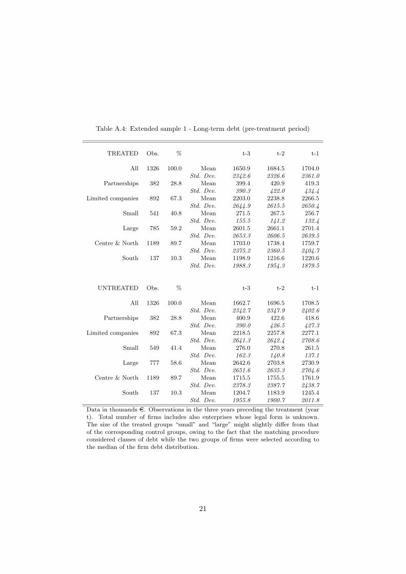
Table A.4: Extended sample 1 - Long-term debt (pre-treatment period)

TREATED Obs. % t-3 t-2 t-1

All 1326 100.0 Mean 1650.9 1684.5 1704.0Std. Dev. 2342.6 2326.6 2361.0

Partnerships 382 28.8 Mean 399.4 420.9 419.3Std. Dev. 390.3 422.0 434.4






UNTREATED Obs. % t-3 t-2 t-1

All 1326 100.0 Mean 1662.7 1696.5 1708.5Std. Dev. 2342.7 2347.9 2402.6

Partnerships 382 28.8 Mean 400.9 422.6 418.6Std. Dev. 390.0 426.5 427.3






Data in thousands e. Observations in the three years preceding the treatment (yeart). Total number of firms includes also enterprises whose legal form is unknown.The size of the treated groups “small” and “large” might slightly differ from thatof the corresponding control groups, owing to the fact that the matching procedureconsidered classes of debt while the two groups of firms were selected according tothe median of the firm debt distribution.

21

Table A.5: Long-term debt growth rate - DID model (baseline estimates)

ENTIRE SAMPLE All Small Large Partnerships Limited companies

dsubsidy 0.016 -0.016 0.024 0.038 0.013(0.025) (0.067) (0.027) (0.083) (0.027)

post -0.028 -0.146* 0.006 -0.081 -0.020(0.028) (0.076) (0.028) (0.057) (0.031)

dsubsidy*post -0.078** -0.016 -0.097** -0.004 -0.086**(0.037) (0.101) (0.038) (0.095) (0.040)

constant 0.067*** 0.086* 0.062*** 0.053 0.066***(0.017) (0.046) (0.018) (0.055) (0.019)

observations 2550 545 2005 210 2240

CENTRE & NORTH All Small Large Partnerships Limited companies

dsubsidy 0.017 -0.031 0.028 0.037 0.015(0.027) (0.077) (0.028) (0.064) (0.030)

post -0.029 -0.164* 0.004 -0.044 -0.025(0.029) (0.083) (0.030) (0.048) (0.033)

dsubsidy*post -0.071* 0.020 -0.093** -0.029 -0.074*(0.039) (0.112) (0.040) (0.073) (0.043)

constant 0.058*** 0.064 0.056*** 0.013 0.058***(0.019) (0.053) (0.019) (0.044) (0.020)

observations 2240 430 1810 180 1970

SOUTH All Small Large Partnerships Limited companies

dsubsidy 0.005 0.044 -0.013 0.038 -0.000(0.074) (0.133) (0.088) (0.428) (0.072)

post -0.019 -0.082 0.021 -0.307 0.015(0.089) (0.186) (0.087) (0.273) (0.096)

dsubsidy*post -0.134 -0.149 -0.131 0.147 -0.175(0.113) (0.232) (0.116) (0.549) (0.116)

constant 0.136*** 0.169* 0.115* 0.289 0.122**(0.048) (0.083) (0.059) (0.269) (0.047)

observations 310 115 195 30 270

Total number of firms includes also enterprises whose legal form is unknown.Robust standard errors in parentheses. *** p<0.01, ** p<0.05, * p<0.1

22

Table A.6: Long term debt growth rate - DID model (subsamples estimates)

RANGE 1 All Small Large Partnerships Limited companies

dsubsidy 0.001 -0.041 0.010 0.043 -0.005(0.032) (0.101) (0.033) (0.116) (0.035)

post -0.008 -0.166* 0.026 -0.074 -0.006(0.036) (0.086) (0.039) (0.084) (0.040)

dsubsidy*post -0.105** -0.027 -0.124** -0.093 -0.107**(0.047) (0.132) (0.050) (0.132) (0.052)

constant 0.064*** 0.072 0.063*** 0.062 0.068***(0.022) (0.064) (0.024) (0.078) (0.024)

observations 1400 240 1160 140 1210


dsubsidy 0.008 -0.057 0.021 0.042 0.003(0.030) (0.101) (0.031) (0.110) (0.033)

post -0.019 -0.217** 0.022 -0.066 -0.011(0.032) (0.085) (0.033) (0.078) (0.035)

dsubsidy*post -0.096** -0.013 -0.117*** -0.093 -0.095**(0.043) (0.127) (0.044) (0.124) (0.046)

constant 0.069*** 0.131** 0.056*** 0.049 0.067***(0.021) (0.064) (0.021) (0.073) (0.022)

observations 1790 290 1500 150 1560


dsubsidy 0.009 -0.038 0.022 0.037 0.005(0.029) (0.077) (0.030) (0.099) (0.031)

post -0.004 -0.168** 0.043 -0.065 0.007(0.032) (0.082) (0.033) (0.069) (0.035)

dsubsidy*post -0.091** 0.051 -0.132*** -0.053 -0.095**(0.042) (0.112) (0.043) (0.113) (0.046)

constant 0.055*** 0.069 0.051** 0.032 0.053**(0.020) (0.052) (0.021) (0.066) (0.021)

observations 1990 425 1565 170 1730

Total number of firms includes also enterprises whose legal form is unknown. Robuststandard errors in parentheses. *** p<0.01, ** p<0.05, * p<0.1. Subsamples are se-lected according to the ratio of subsidized loans over total bank credit (three ranges areconsidered: range 1, 10%-75%; range 2, 10%-100%; range 3, 10%-200%).

23

Table A.7: Long term debt growth rate - DID model (extended sample estimates)

ENTIRE SAMPLE All Small Large Partnerships Limited companies

dsubsidy 0.011 0.005 0.014 0.010 0.012(0.011) (0.017) (0.014) (0.017) (0.014)

post -0.051*** -0.075*** -0.034* -0.065*** -0.041**(0.014) (0.022) (0.018) (0.022) (0.018)

dsubsidy*post -0.043** -0.005 -0.070*** -0.016 -0.056**(0.018) (0.028) (0.023) (0.029) (0.023)

constant 0.065*** 0.042*** 0.082*** 0.050*** 0.071***(0.008) (0.012) (0.010) (0.012) (0.010)

observations 10608 4360 6248 3056 7136

CENTRE & NORTH All Small Large Partnerships Limited companies

dsubsidy 0.010 0.004 0.014 0.010 0.010(0.012) (0.018) (0.015) (0.018) (0.015)

post -0.051*** -0.081*** -0.030 -0.063*** -0.042**(0.014) (0.023) (0.019) (0.024) (0.019)

dsubsidy*post -0.037* 0.013 -0.070*** -0.019 -0.046*(0.019) (0.030) (0.024) (0.031) (0.024)

constant 0.065*** 0.037*** 0.083*** 0.051*** 0.070***(0.008) (0.013) (0.010) (0.012) (0.010)

observations 9512 3776 5736 2808 6360

SOUTH All Small Large Partnerships Limited companies

dsubsidy 0.015 0.015 0.014 0.006 0.021(0.034) (0.047) (0.048) (0.065) (0.042)

post -0.055 -0.039 -0.074* -0.085 -0.033(0.041) (0.067) (0.040) (0.056) (0.054)

dsubsidy*post -0.096* -0.125 -0.062 0.016 -0.139**(0.054) (0.084) (0.064) (0.094) (0.069)

constant 0.072*** 0.073** 0.070** 0.047 0.081***(0.022) (0.032) (0.031) (0.045) (0.028)

observations 1096 584 512 248 776


24

Tab

leA

.8:

Lon

gte

rmde

btgr

owth

rate

-D

IDm

odel

(ext

ende

dsa

mpl

ees

tim

ates

wit

hdu

mm

ySo

uth

inte

ract

ions

)

EN

TIR

ESA

MP

LE

All

Sm

all

Larg

eP

art

ner

ship

sL

imit

edco

mpanie

sA

llSm

all

Larg

eP

art

ner

ship

sL

imit

edco

mpanie

s

dsu

bsi

dy

0.0

11

0.0

05

0.0

14

0.0

10

0.0

12

0.0

10

0.0

04

0.0

14

0.0

10

0.0

10

(0.0

11)

(0.0

17)

(0.0

14)

(0.0

17)

(0.0

14)

(0.0

12)

(0.0

18)

(0.0

15)

(0.0

18)

(0.0

15)

dsu

bsi

dy*South

0.0

04

0.0

12

-0.0

00

-0.0

04

0.0

11

(0.0

35)

(0.0

50)

(0.0

50)

(0.0

67)

(0.0

45)

post

-0.0

51***

-0.0

75***

-0.0

34*

-0.0

65***

-0.0

41**

-0.0

51***

-0.0

81***

-0.0

30

-0.0

63***

-0.0

42**

(0.0

14)

(0.0

22)

(0.0

18)

(0.0

22)

(0.0

18)

(0.0

14)

(0.0

23)

(0.0

19)

(0.0

24)

(0.0

19)

post

*South

-0.0

04

0.0

42

-0.0

43

-0.0

22

0.0

09

(0.0

43)

(0.0

70)

(0.0

44)

(0.0

60)

(0.0

57)

dsu

bsi

dy*p

ost

-0.0

38**

0.0

01

-0.0

66***

-0.0

16

-0.0

49**

-0.0

37*

0.0

13

-0.0

70***

-0.0

19

-0.0

46*

(0.0

18)

(0.0

29)

(0.0

23)

(0.0

29)

(0.0

23)

(0.0

19)

(0.0

30)

(0.0

24)

(0.0

31)

(0.0

24)

South

0.0

07

0.0

36

-0.0

13

-0.0

03

0.0

11

(0.0

24)

(0.0

34)

(0.0

32)

(0.0

46)

(0.0

30)

dsu

bsi

dy*p

ost

*South

-0.0

52*

-0.0

49

-0.0

49

0.0

06

-0.0

62*

-0.0

59

-0.1

39

0.0

08

0.0

34

-0.0

93

(0.0

31)

(0.0

42)

(0.0

45)

(0.0

56)

(0.0

38)

(0.0

57)

(0.0

89)

(0.0

69)

(0.0

98)

(0.0

73)

const

ant

0.0

65***

0.0

42***

0.0

82***

0.0

50***

0.0

71***

0.0

65***

0.0

37***

0.0

83***

0.0

51***

0.0

70***

(0.0

08)

(0.0

12)

(0.0

10)

(0.0

12)

(0.0

10)

(0.0

08)

(0.0

13)

(0.0

10)

(0.0

12)

(0.0

10)

obse

rvati

ons

10608

4360

6248

3056

7136

10608

4360

6248

3056

7136

Tota

lnum

ber

of

firm

sin

cludes

als

oen

terp

rise

sw

hose

legal

form

isunknow

n.

Robust

standard

erro

rsin

pare

nth

eses

.***

p<

0.0

1,

**

p<

0.0

5,

*p<

0.1

25

Tab

leA

.9:

Lon

gte

rmde

btgr

owth

rate

-D

IDm

odel

(ext

ende

dsa

mpl

ees

tim

ates

acco

rdin

gto

the

finan

cial

tens

ion

indi

cato

r)

AL

LSM

AL

LL

AR

GE

PA

RT

NE

RSH

IPS

LIM

ITE

DC

OM

PA

NIE

S

low

-ten

shi-

tens

low

-ten

shi-

tens

low

-ten

shi-

tens

low

-ten

shi-

tens

low

-ten

shi-

tens

dsu

bsi

dy

0.0

18

0.0

05

-0.0

18

0.0

24

0.0

41**

-0.0

15

0.0

03

0.0

15

0.0

23

-0.0

01

(0.0

16)

(0.0

15)

(0.0

27)

(0.0

22)

(0.0

19)

(0.0

21)

(0.0

29)

(0.0

22)

(0.0

19)

(0.0

21)

post

-0.0

10

-0.0

87***

-0.0

51

-0.0

90***

0.0

12

-0.0

84***

-0.0

37

-0.0

80***

-0.0

02

-0.0

82***

(0.0

21)

(0.0

18)

(0.0

39)

(0.0

25)

(0.0

25)

(0.0

25)

(0.0

42)

(0.0

25)

(0.0

25)

(0.0

25)

dsu

bsi

dy*p

ost

-0.0

70***

-0.0

21

0.0

15

-0.0

26

-0.1

17***

-0.0

18

-0.0

28

-0.0

13

-0.0

81**

-0.0

28

(0.0

26)

(0.0

24)

(0.0

47)

(0.0

36)

(0.0

32)

(0.0

33)

(0.0

51)

(0.0

36)

(0.0

32)

(0.0

33)

const

ant

0.0

46***

0.0

82***

0.0

41**

0.0

43***

0.0

48***

0.1

18***

0.0

45**

0.0

54***

0.0

47***

0.0

97***

(0.0

11)

(0.0

11)

(0.0

21)

(0.0

14)

(0.0

12)

(0.0

15)

(0.0

21)

(0.0

14)

(0.0

13)

(0.0

15)

Obse

rvati

ons

5024

5584

1808

2552

3216

3032

1168

1888

3660

3476

Tota

lnum

ber

of

firm

sin

cludes

als

oen

terp

rise

sw

hose

legal

form

isunknow

n.

The

financi

al

tensi

on

ism

easu

red

by

the

rati

oof

short

term

cred

itact

ually

dis

burs

edand

short

term

cred

itgra

nte

dby

banks;

we

split

the

firm

sin

totw

ogro

ups

at

the

med

ian

of

the

indic

ato

r.R

obust

standard

erro

rsin

pare

nth

eses

.***

p<

0.0

1,

**

p<

0.0

5,

*p<

0.1

26

Tab

leA

.10:

Lon

gte

rmde

btgr

owth

rate

-D

IDm

odel

(ext

ende

dsa

mpl

eses

tim

ates

acco

rdin

gto

the

finan

cial

tens

ion

indi

cato

r)

AL

LSM

AL

LL

AR

GE

PA

RT

NE

RSH

IPS

LIM

ITE

DC

OM

PA

NIE

S

low

-ten

shi-

tens

low

-ten

shi-

tens

low

-ten

shi-

tens

low

-ten

shi-

tens

low

-ten

shi-

tens

dsu

bsi

dy

0.0

11

0.0

18

-0.0

13

0.0

47

0.0

25

-0.0

18

0.0

02

0.0

25

0.0

15

0.0

04

(0.0

12)

(0.0

23)

(0.0

21)

(0.0

30)

(0.0

15)

(0.0

37)

(0.0

23)

(0.0

27)

(0.0

15)

(0.0

37)

post

-0.0

24

-0.1

21***

-0.0

59**

-0.1

01***

-0.0

04

-0.1

45***

-0.0

44

-0.0

94***

-0.0

17

-0.1

32***

(0.0

16)

(0.0

24)

(0.0

29)

(0.0

32)

(0.0

20)

(0.0

37)

(0.0

30)

(0.0

32)

(0.0

20)

(0.0

38)

dsu

bsi

dy*p

ost

-0.0

54***

-0.0

29

0.0

10

-0.0

47

-0.0

89***

-0.0

08

-0.0

33

0.0

05

-0.0

61**

-0.0

48

(0.0

21)

(0.0

36)

(0.0

36)

(0.0

48)

(0.0

25)

(0.0

55)

(0.0

38)

(0.0

47)

(0.0

25)

(0.0

55)

const

ant

0.0

58***

0.0

86***

0.0

41***

0.0

43**

0.0

67***

0.1

40***

0.0

51***

0.0

49***

0.0

60***

0.1

16***

(0.0

09)

(0.0

15)

(0.0

15)

(0.0

18)

(0.0

10)

(0.0

25)

(0.0

16)

(0.0

18)

(0.0

10)

(0.0

25)

Obse

rvati

ons

7940

2668

2868

1492

5072

1176

1912

1144

5740

1396

Tota

lnum

ber

of

firm

sin

cludes

als

oen

terp

rise

sw

hose

legal

form

isunknow

n.

The

financi

al

tensi

on

ism

easu

red

by

the

rati

oof

short

term

cred

itact

ually

dis

burs

edand

short

term

cred

itgra

nte

dby

banks;

we

split

the

firm

sin

totw

ogro

ups

at

the

80th

per

centi

leof

the

indic

ato

r’s

dis

trib

uti

on.

Robust

standard

erro

rsin

pare

nth

eses

.***

p<

0.0

1,

**

p<

0.0

5,

*p<

0.1

27

Table A.11: Long term debt level - GMM model (baseline sample:3 years treatment)

Fixed Effects GMM-DIF GMM-SYS

ALL (1) (2) (1) (2) (1) (2)

debtt−1 0.348*** 0.350*** 0.416*** 0.507*** 1.047*** 1.000***(0.023) (0.023) (0.134) (0.168) (0.047) (0.041)

post -0.071** -0.037* -0.099*** -0.070** -0.094*** -0.136***(0.031) (0.020) (0.033) (0.030) (0.035) (0.028)

observations 2053 2053 1619 1619 2053 2053firms 432 432 432 432 432 432

SMALL (1) (2) (1) (2) (1) (2)

debtt−1 0.299*** 0.304*** 0.467*** 0.381*** 1.014*** 1.097***(0.053) (0.053) (0.114) (0.137) (0.184) (0.166)

post -0.034 -0.067 -0.167* -0.172*** 0.037 -0.029(0.079) (0.051) (0.097) (0.063) (0.124) (0.087)


LARGE (1) (2) (1) (2) (1) (2)

debtt−1 0.363*** 0.365*** 0.543*** 0.606*** 0.955*** 0.939***(0.026) (0.026) (0.108) (0.192) (0.079) (0.076)

post -0.055* -0.031 -0.087** -0.065* -0.105*** -0.135***(0.033) (0.022) (0.035) (0.038) (0.035) (0.029)


PARTNERSHIPS (1) (2) (1) (2) (1) (2)

debtt−1 0.289*** 0.286*** 0.011 -0.441** 1.025*** 1.029***(0.076) (0.075) (0.558) (0.184) (0.072) (0.081)

post 0.053 0.067 0.039 0.058 0.007 0.015(0.092) (0.059) (0.190) (0.066) (0.122) (0.080)


LIMITED COMPANIES (1) (2) (1) (2) (1) (2)

debtt−1 0.352*** 0.353*** 0.379*** 0.511*** 1.068*** 1.012***(0.025) (0.025) (0.136) (0.162) (0.053) (0.044)

post -0.040 -0.048** -0.108*** -0.082*** -0.105*** -0.153***(0.034) (0.022) (0.034) (0.031) (0.037) (0.030)


Total number of firms includes also enterprises whose legal form is unknown. Standard errors inparentheses. *** p<0.01, ** p<0.05, * p<0.1. (1) Year dummies included. (2) Year dummiesexcluded.

28

Table A.12: Long term debt level - GMM model (extended sample:2 years treat-ment)

Fixed Effects GMM-DIF GMM-SYS

ALL (1) (2) (1) (2) (1) (2)

debtt−1 0.259*** 0.260*** 0.495*** 0.442*** 0.885*** 0.868***(0.019) (0.019) (0.119) (0.126) (0.040) (0.035)

post -0.002 0.004 -0.061*** -0.034* -0.097*** -0.075***(0.020) (0.015) (0.021) (0.019) (0.024) (0.018)


SMALL (1) (2) (1) (2) (1) (2)

debtt−1 0.209*** 0.204*** 0.584*** 0.484** 0.696*** 0.693***(0.043) (0.043) (0.107) (0.203) (0.077) (0.075)

post 0.032 -0.038 -0.006 -0.057 0.052 -0.026(0.044) (0.031) (0.053) (0.035) (0.058) (0.036)


LARGE (1) (2) (1) (2) (1) (2)

debtt−1 0.266*** 0.272*** 0.574*** 0.511*** 0.816*** 0.782***(0.021) (0.021) (0.073) (0.104) (0.067) (0.061)

post 0.000 0.016 -0.072*** -0.037* -0.104*** -0.078***(0.023) (0.017) (0.023) (0.021) (0.027) (0.021)


PARTNERSHIPS (1) (2) (1) (2) (1) (2)

debtt−1 0.262*** 0.251*** 0.776** 0.157 0.914*** 0.871***(0.059) (0.059) (0.316) (0.405) (0.056) (0.065)

post 0.068 0.019 -0.047 0.021 -0.036 -0.012(0.053) (0.038) (0.050) (0.050) (0.048) (0.043)


LIMITED COMPANIES (1) (2) (1) (2) (1) (2)

debtt−1 0.259*** 0.261*** 0.511*** 0.454*** 0.890*** 0.869***(0.021) (0.021) (0.118) (0.138) (0.049) (0.041)

post 0.007 0.001 -0.069*** -0.040* -0.105*** -0.083***(0.023) (0.017) (0.023) (0.021) (0.027) (0.019)


Total number of firms includes also enterprises whose legal form is unknown. Standard errors inparentheses. *** p<0.01, ** p<0.05, * p<0.1. (1) Year dummies included. (2) Year dummiesexcluded. 29

Table A.13: Long term debt growth rate - DID model (subsidized firms only, 2years treatment)

All Small Large Partnerships Limited companies

dsubsidy -0.028 -0.087*** 0.011 -0.060 -0.019(0.022) (0.033) (0.028) (0.039) (0.027)

post -0.019 -0.030 -0.011 -0.011 -0.022(0.019) (0.028) (0.024) (0.031) (0.024)

dsubsidy*post -0.054** -0.047 -0.062* -0.021 -0.058*(0.027) (0.042) (0.034) (0.050) (0.033)

constant 0.078*** 0.058*** 0.093*** 0.073*** 0.077***(0.016) (0.022) (0.019) (0.025) (0.019)

observations 5134 2083 3051 1293 3520


Table A.14: Investments over assets - DID model

All Small Large

dsubsidy 0.015* 0.021 0.011(0.008) (0.013) (0.009)

post -0.003 -0.016** 0.012(0.006) (0.007) (0.009)

dsubsidy*post 0.009 0.017 0.001(0.012) (0.019) (0.015)

constant 0.022*** 0.032*** 0.011***(0.005) (0.008) (0.003)

observations 1116 544 572

Robust standard errors in parentheses. *** p<0.01,** p<0.05, * p<0.1

30

financial subsidies and bank lending: substitutes or ... subsidies and bank lending: substitutes or...

Documents