Network Formation with Local Complements

and Global Substitutes:The Case of R&D Networks

Chih-Sheng Hsieh, Michael D. Konig and Xiaodong Liu

Second Annual NSF Conference on Network Science in EconomicsStanford University

23rd April 2016

1/46

Research Projects

A. Innovation Networks and Technology Diffusion

A1. ”R&D Networks: Theory, Empirics and Policy Implications”

A2. ”Network Formation with Local Complements and Global

Substitutes”

A3. ”Dynamic R&D Networks with Process and Product Innovations”A4. ”Endogenous Technology Cycles in Dynamic R&D Networks”A5. ”Coauthorship Networks and Research Output”

B. Heterogeneous Firm Dynamics and ProductionNetworks

B1. ”Peer Effects in FDI Networks and Technology Spillovers”B2. ”Endogenous Production Networks”B3. ”From Imitation to Innovation: Where is All That Chinese R&D

Going?”

C. Game Theoretic Models of Conflict in Networks

C1. ”Networks and Conflicts: Theory and Evidence from Rebel

Groups in Africa”C2. ”Conflict Networks in Syria and Iraq”C3. ”The Arab Spring and the Spread of Revolutions in Online Social

Networks”

2/46

Introduction

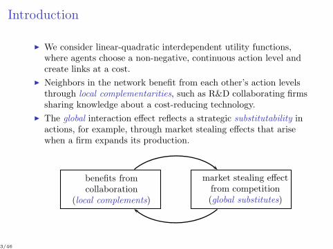
We consider linear-quadratic interdependent utility functions,where agents choose a non-negative, continuous action level andcreate links at a cost.

Neighbors in the network benefit from each other’s action levelsthrough local complementarities, such as R&D collaborating firmssharing knowledge about a cost-reducing technology.

The global interaction effect reflects a strategic substitutability inactions, for example, through market stealing effects that arisewhen a firm expands its production.

benefits fromcollaboration

(local complements)

market stealing effectfrom competition(global substitutes)

3/46

Contribution: theory

We provide a general and complete characterization of bothequilibrium networks and endogenous production choices in theform of a Gibbs measure.

Equilibrium networks can be characterized as inhomogenous

random graphs, and the stochastically stable networks are nested

split graphs.1

We find a sharp transition from sparse to dense networks, and lowand high output levels, respectively, with decreasing linking costs.

Moreover, there exists an intermediate range of the linking costfor which multiple equilibria arise. The equilibrium selection is apath dependent process characterized by hysteresis.

We then bring the model to the data by analyzing a uniquedataset of R&D collaborations matched to firm’s balance sheetsand patents.

1A network exhibits nestedness if the neighborhood of a node is contained in theneighborhoods of the nodes with higher degrees.

4/46

Contribution: econometrics

The theoretical characterization of the stationary states via aGibbs measure allows us to estimate the model’s parametersusing three alternative estimation algorithms:

(i) a Bayesian maximum likelihood method (MLE),(ii) a double Metropolis-Hastings Markov Chain (DMH) Monte Carlo

algorithm,(iii) or an adaptive exchange algorithm (AEX).

This generalizes the models proposed in Snijders (2001)2 andMele (2010)3 whho also use a Gibbs measure to characterize thestationary states, but here both, the action choices (eithercontinuous or discrete) as well as the linking decisions are fullyendogenized.

Our model is also closely related to Badev (2013)4 who analyzesthe formation of binary choices and network links.

2Tom A.B. Snijders. “The Statistical Evaluation of Social Network Dynamics”.Sociological Methodology 31.1 (2001), pp. 361–395.

3A. Mele. “Segregation in Social Networks: Theory, Estimation and Policy”. NETInstitute Working Paper 10-16. 2010.

4Anton Badev. “Discrete games in endogenous networks: Theory and policy”.University of Pennsylvania Working Paper PSC 13–05 (2013).

5/46

Contribution: policy

We use our estimated model to investigate the impact ofexogenous shocks on the network (cf. dynamic “key player

analysis”),5 and find that the exit of Pfizer would lead to areduction in welfare of 9.3%.

Our framework also allows us to study mergers and acquisitions

(M&As), and their impact on welfare.6 Our results show that amerger between Cubist Pharmaceuticals and Novartis wouldresult in a welfare loss of 2.9%.

Finally, we investigate the impact of subsidizing R&D

collaboration costs of selected pairs of firms.7 We find thatsubsidizing a collaboration between Isis Pharmaceuticals Inc.

and Allergan Inc. would increase welfare by 0.8%.

5Yves Zenou. “Key Players”. Oxford Handbook on the Economics of Networks, Y.Bramoulle, B. Rogers and A. Galeotti (Eds.), Oxford University Press (2015).

6Joseph Farrell and Carl Shapiro. “Horizontal mergers: an equilibrium analysis”.The American Economic Review (1990), pp. 107–126.

7Cf. e.g. Linda Cohen. “When can government subsidize research joint ventures?Politics, economics, and limits to technology policy”. The American EconomicReview (1994), pp. 159–163.

6/46

The Model

The standard inverse demand for firm i producing quantity qi is

pi = a− qi − b∑

j 6=i

qj . (1)

Firms can reduce their costs for production by investing intoR&D as well as by establishing an R&D collaboration withanother firm.

The amount of this cost reduction depends on the effort ei that afirm i and the effort ej that its R&D collaboration partnersj ∈ Ni invest into the collaboration.

Given the effort level ei ∈ R+, marginal cost ci of firm i is givenby

ci = c− αei − β

n∑

j=1

aijej, (2)

where aij = 1 if firms i and j set up a collaboration (0 otherwise)and aii = 0.

7/46

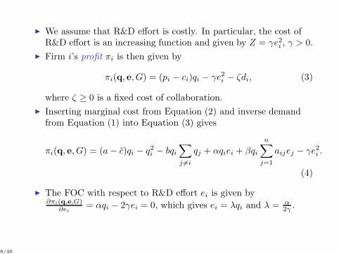
We assume that R&D effort is costly. In particular, the cost ofR&D effort is an increasing function and given by Z = γe2i , γ > 0.

Firm i’s profit πi is then given by

πi(q, e, G) = (pi − ci)qi − γe2i − ζdi, (3)

where ζ ≥ 0 is a fixed cost of collaboration.

Inserting marginal cost from Equation (2) and inverse demandfrom Equation (1) into Equation (3) gives

πi(q, e, G) = (a− c)qi − q2i − bqi∑

j 6=i

qj + αqiei + βqi

n∑

j=1

aijej − γe2i .

(4)

The FOC with respect to R&D effort ei is given by∂πi(q,e,G)

∂ei= αqi − 2γei = 0, which gives ei = λqi and λ = α

2γ .

8/46

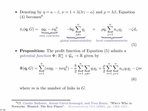
Denoting by η = a− c, ν = 1 + λ(λγ − α) and ρ = λβ, Equation(4) becomes8

πi(q, G) = ηqi − νq2i︸ ︷︷ ︸

own concavity

−bqi

n∑

j 6=i

qj

︸ ︷︷ ︸

global substitutability

+ ρqi

n∑

j=1

aijqj

︸ ︷︷ ︸

local complementarity

−ζdi.

(5)

Proposition: The profit function of Equation (5) admits apotential function Φ: Rn+ × Gn → R given by

Φ(q, G) =

n∑

i=1

(nηqi − nνq2i )−b

2

n∑

i=1

∑

j 6=i

qiqj +ρ

2

n∑

i=1

n∑

j=1

aijqiqj − ζm

(6)

where m is the number of links in G.

8Cf. Coralio Ballester, Antoni Calvo-Armengol, and Yves Zenou. “Who’s Who inNetworks. Wanted: The Key Player”. Econometrica 74.5 (2006), pp. 1403–1417.

9/46

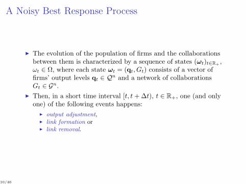
A Noisy Best Response Process

The evolution of the population of firms and the collaborationsbetween them is characterized by a sequence of states (ωt)t∈R+ ,ωt ∈ Ω, where each state ωt = (qt, Gt) consists of a vector offirms’ output levels qt ∈ Qn and a network of collaborationsGt ∈ Gn.

Then, in a short time interval [t, t+∆t), t ∈ R+, one (and onlyone) of the following events happens:

output adjustment, link formation or link removal.

10/46

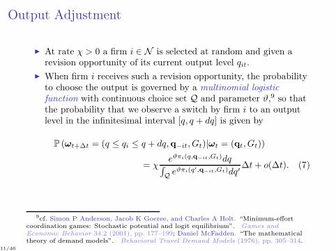
Output Adjustment

At rate χ > 0 a firm i ∈ N is selected at random and given arevision opportunity of its current output level qit.

When firm i receives such a revision opportunity, the probabilityto choose the output is governed by a multinomial logistic

function with continuous choice set Q and parameter ϑ,9 so thatthe probability that we observe a switch by firm i to an outputlevel in the infinitesimal interval [q, q + dq] is given by

P (ωt+∆t = (q ≤ qi ≤ q + dq,q−it, Gt)|ωt = (qt, Gt))

= χeϑπi(q,q−it,Gt)dq

∫

Q eϑπi(q′,q−it,Gt)dq′∆t+ o(∆t). (7)

9cf. Simon P Anderson, Jacob K Goeree, and Charles A Holt. “Minimum-effortcoordination games: Stochastic potential and logit equilibrium”. Games andEconomic Behavior 34.2 (2001), pp. 177–199; Daniel McFadden. “The mathematicaltheory of demand models”. Behavioral Travel Demand Models (1976), pp. 305–314.

11/46

Link Formation

With rate λ > 0 a pair of firms ij which is not already connectedreceives an opportunity to form a link.

The formation of a link depends on the marginal payoff the firmsreceive from the link plus an additive pairwise i.i.d. error termεij,t.

The probability that link ij is created is then given by

P (ωt+∆t = (qt, Gt + ij)|ωt−1 = (q, Gt))

= λ P (πi(qt, Gt + ij)− πi(qt, Gt) + εij,t > 0

∩πj(qt, Gt + ij)− πj(qt, Gt) + εij,t > 0)∆t+ o(∆t)

= λeϑΦ(qt,Gt+ij)

eϑΦ(qt,Gt+ij) + eϑΦ(qt,Gt)∆t+ o(∆t),

where we have used the fact that πi(qt, Gt + ij)− πi(qt, Gt) =πj(qt, Gt + ij)− πj(qt, Gt) = Φ(qt, Gt + ij)− Φ(qt, Gt) andassumed that the error term εij,t is i.i. logistically distributed.

12/46

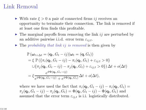
Link Removal

With rate ξ > 0 a pair of connected firms ij receives anopportunity to terminate their connection. The link is removed ifat least one firm finds this profitable.

The marginal payoffs from removing the link ij are perturbed byan additive pairwise i.i.d. error term εij,t.

The probability that link ij is removed is then given by

P (ωt+∆t = (qt, Gt − ij)|ωt = (q, Gt))

= ξ P (πi(qt, Gt − ij)− πi(qt, Gt) + εij,t > 0

∪πj(qt, Gt − ij)− πj(qt, Gt) + εij,t > 0)∆t+ o(∆t)

= ξeϑΦ(qt,Gt−ij)

eϑΦ(qt,Gt−ij) + eϑΦ(qt,Gt)∆t+ o(∆t),

where we have used the fact that πi(qt, Gt − ij)− πi(qt, Gt) =πj(qt, Gt − ij)− πj(qt, Gt) = Φ(qt, Gt − ij)− Φ(qt, Gt) andassumed that the error term εij,t is i.i. logistically distributed.

13/46

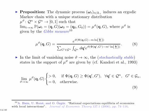
Proposition: The dynamic process (ωt)t∈R+ induces an ergodicMarkov chain with a unique stationary distributionµϑ : Qn × Gn → [0, 1] such thatlimt→∞ P(ωt = (q, G)|ω0 = (q0, G0)) = µϑ(q, G), where µϑ isgiven by the Gibbs measure10

µϑ(q, G) =eϑ(Φ(q,G)−m ln( ξ

λ ))

∑

G′∈Gn

∫

Qn dq′eϑ(Φ(q′,G′)−m′ ln( ξλ ))

. (8)

In the limit of vanishing noise ϑ → ∞, the (stochastically stable)states in the support of µϑ are given by (cf. Kandori et al., 1993)

limϑ→∞

µϑ(q, G)

> 0, if Φ(q, G) ≥ Φ(q′, G′), ∀q′ ∈ Qn, G′ ∈ Gn,

= 0, otherwise.

(9)

10A. Bisin, U. Horst, and O. Ozgur. “Rational expectations equilibria of economieswith local interactions”. Journal of Economic Theory 127.1 (2006), pp. 74–116.

14/46

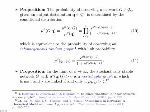
Proposition: The probability of observing a network G ∈ Gn,given an output distribution q ∈ Qn is determined by theconditional distribution

µϑ(G|q) =µϑ(q, G)

µϑ(q)=

n∏

i<j

eϑaij(ρqiqj−ζ)

1 + eϑ(ρqiqj−ζ), (10)

which is equivalent to the probability of observing aninhomogeneous random graph11 with link probability

pϑ(qi, qj) =eϑ(ρqiqj−ζ)

1 + eϑ(ρqiqj−ζ). (11)

Proposition: In the limit of ϑ → ∞, the stochastically stablenetwork G with µ∗(q, G) > 0 is a nested split graph in whichfirms i and j are linked if and only if ρqiqj > ζ.12

11B. Bollobas, S. Janson, and O. Riordan. “The phase transition in inhomogeneousrandom graphs”. Random Structures & Algorithms 31.1 (2007), pp. 3–122.

12Cf. e.g. M. Konig, C. Tessone, and Y. Zenou. “Nestedness in Networks: ATheoretical Model and Some Applications”. Theoretical Economics 9 (2014),pp. 695–752.

15/46

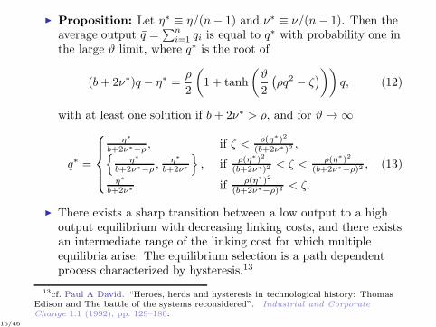
Proposition: Let η∗ ≡ η/(n− 1) and ν∗ ≡ ν/(n− 1). Then theaverage output q =

∑ni=1 qi is equal to q∗ with probability one in

the large ϑ limit, where q∗ is the root of

(b+ 2ν∗)q − η∗ =ρ

2

(

1 + tanh

(ϑ

2

(ρq2 − ζ

)))

q, (12)

with at least one solution if b + 2ν∗ > ρ, and for ϑ → ∞

q∗ =

η∗

b+2ν∗−ρ , if ζ < ρ(η∗)2

(b+2ν∗)2 ,η∗

b+2ν∗−ρ ,η∗

b+2ν∗

, if ρ(η∗)2

(b+2ν∗)2 < ζ < ρ(η∗)2

(b+2ν∗−ρ)2 ,

η∗

b+2ν∗ , if ρ(η∗)2

(b+2ν∗−ρ)2 < ζ.

(13)

There exists a sharp transition between a low output to a highoutput equilibrium with decreasing linking costs, and there existsan intermediate range of the linking cost for which multipleequilibria arise. The equilibrium selection is a path dependentprocess characterized by hysteresis.13

13cf. Paul A David. “Heroes, herds and hysteresis in technological history: ThomasEdison and The battle of the systems reconsidered”. Industrial and CorporateChange 1.1 (1992), pp. 129–180.

16/46

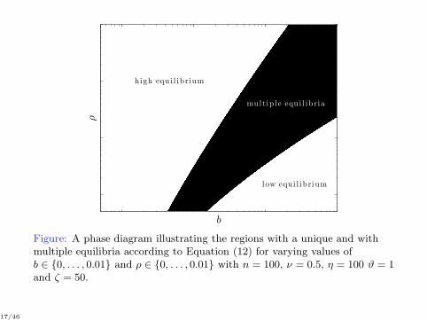
ρ

b

high equi l ibrium

multip l e equi l ibria

low equi l ibrium

Figure: A phase diagram illustrating the regions with a unique and withmultiple equilibria according to Equation (12) for varying values ofb ∈ 0, . . . , 0.01 and ρ ∈ 0, . . . , 0.01 with n = 100, ν = 0.5, η = 100 ϑ = 1and ζ = 50.

17/46

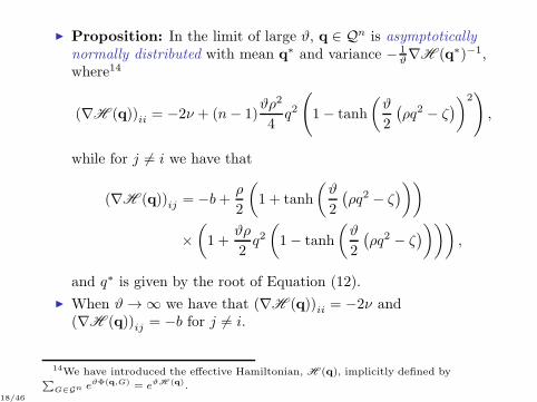
Proposition: In the limit of large ϑ, q ∈ Qn is asymptotically

normally distributed with mean q∗ and variance − 1ϑ∇H (q∗)−1,

where14

(∇H (q))ii = −2ν + (n− 1)ϑρ2

4q2

(

1− tanh

(ϑ

2

(ρq2 − ζ

))2)

,

while for j 6= i we have that

(∇H (q))ij = −b+ρ

2

(

1 + tanh

(ϑ

2

(ρq2 − ζ

)))

×

(

1 +ϑρ

2q2(

1− tanh

(ϑ

2

(ρq2 − ζ

))))

,

and q∗ is given by the root of Equation (12).

When ϑ → ∞ we have that (∇H (q))ii = −2ν and(∇H (q))ij = −b for j 6= i.

14We have introduced the effective Hamiltonian, H (q), implicitly defined by∑

G∈Gn eϑΦ(q,G) = eϑH (q).

18/46

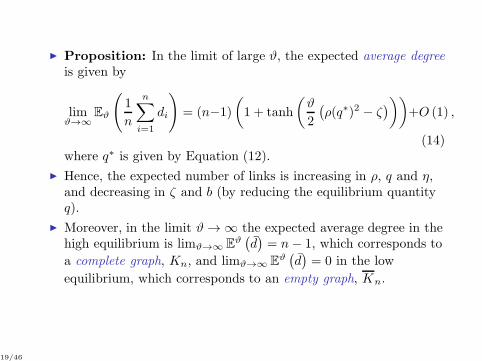
Proposition: In the limit of large ϑ, the expected average degree

is given by

limϑ→∞

Eϑ

(

1

n

n∑

i=1

di

)

= (n−1)

(

1 + tanh

(ϑ

2

(ρ(q∗)2 − ζ

)))

+O (1) ,

(14)where q∗ is given by Equation (12).

Hence, the expected number of links is increasing in ρ, q and η,and decreasing in ζ and b (by reducing the equilibrium quantityq).

Moreover, in the limit ϑ → ∞ the expected average degree in thehigh equilibrium is limϑ→∞ E

ϑ(d)= n− 1, which corresponds to

a complete graph, Kn, and limϑ→∞ Eϑ(d)= 0 in the low

equilibrium, which corresponds to an empty graph, Kn.

19/46

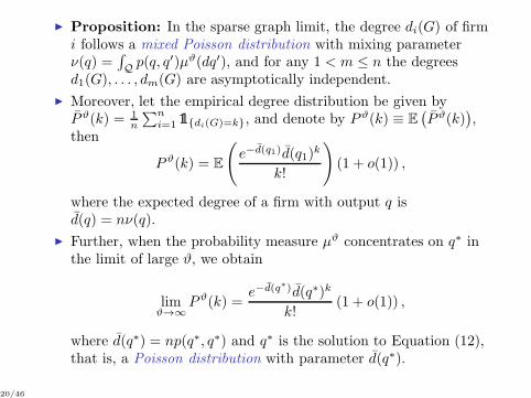
Proposition: In the sparse graph limit, the degree di(G) of firmi follows a mixed Poisson distribution with mixing parameterν(q) =

∫

Qp(q, q′)µϑ(dq′), and for any 1 < m ≤ n the degrees

d1(G), . . . , dm(G) are asymptotically independent.

Moreover, let the empirical degree distribution be given byPϑ(k) = 1

n

∑ni=1 1di(G)=k, and denote by Pϑ(k) ≡ E

(Pϑ(k)

),

then

Pϑ(k) = E

(

e−d(q1)d(q1)k

k!

)

(1 + o(1)) ,

where the expected degree of a firm with output q isd(q) = nν(q).

Further, when the probability measure µϑ concentrates on q∗ inthe limit of large ϑ, we obtain

limϑ→∞

Pϑ(k) =e−d(q

∗)d(q∗)k

k!(1 + o(1)) ,

where d(q∗) = np(q∗, q∗) and q∗ is the solution to Equation (12),that is, a Poisson distribution with parameter d(q∗).

20/46

Introducing Heterogeneity

First, consider ex ante heterogeneity among firms in the variableproduction cost ci ≥ 0 for i = 1, . . . , n.15

Similarly to above, we can characterize the equilibrium statesusing a Gibbs measure.

Moreover, the equilibrium networks are nested split graphs inwhich firms with lower marginal costs are more central.

Further, when the firms’ productivities are Pareto distributed(more precisely, a stable distribution with power-law tail)16 thenalso the firms’ output levels follow a Pareto distribution,consistent with the empirical data.17

15See also A.V. Banerjee and E. Duflo. “Growth theory through the lens ofdevelopment economics”. Handbook of Economic growth 1 (2005), pp. 473–552.

16John P Nolan. Stable distributions: Models for Heavy Tailed Data. 2014.17Cf. e.g. Xavier Gabaix. “Power Laws in Economics and Finance”. Annual Review

of Economics 1.1 (2009), pp. 255–294; Michael D. Konig, Jan Lorenz, andFabrizio Zilibotti. “Innovation vs. Imitation and the Evolution of ProductivityDistributions”. CEPR Discussion Paper No. 8843 (2012).

21/46

Second, assume that firms with higher productivity incur lowercollaboration costs, e.g. ζij =

ζsisj

, where si > 0 is the

productivity or efficiency of firm i.

Then one can show that a similar equilibrium characterizationusing a Gibbs measure is possible.

Moreover, in the special case of firm i’s productivity si beingPareto distributed, one can show that the degree distribution alsofollows a Pareto distribution,18 confirming previous empiricalstudies of R&D networks.19

Under the assumptions of a power-law productivity distribution,we can generate two-vertex and three-vertex degree correlations.

18In particular, assume that the productivities s are distributed as a power-law s−γ

with exponent γ. Then on can show that the asymptotic degree distribution is also

power-law distributed, P (k) ∼ k−

γγ−1 , with exponent γ

γ−1 .19e.g. Walter W. Powell et al. “Network Dynamics and Field Evolution: The Growth

of Interorganizational Collaboration in the Life Sciences”. American Journal ofSociology 110.4 (2005), pp. 1132–1205; Brigitte Gay and Bernard Dousset. “Innovationand Network Structural Dynamics: Study of the Alliance Network of a Major Sector ofthe Biotechnology Industry”. Research Policy (2005), pp. 1457–1475.

22/46

Third, assume that there are heterogeneous spillovers betweencollaborating firms depending on their technology portfolios20.

For example, assume that firms can only benefit fromcollaborations if they have at least one technology in common,and technologies are randomly distributed across firms.

Then one can show that our model is a generalization of arandom intersection graph,21 for which power-law degreedistributions, a decaying clustering degree distribution andpositive degree correlations can be obtained (assortativity).22

20Cf. R. Griffith, S. Redding, and J. Van Reenen. “R&D and Absorptive Capacity:Theory and Empirical Evidence”. Scandinavian Journal of Economics 105.1 (2003),pp. 99–118.

21Cf. KB Singer-Cohen. “Random intersection graphs”. PhD thesis. PhD thesis,Department of Mathematical Sciences, The Johns Hopkins University, 1995;Maria Deijfen and Willemien Kets. “Random intersection graphs with tunable degreedistribution and clustering”. Probability in the Engineering and InformationalSciences 23.04 (2009), pp. 661–674; Mark E.J. Newman. “Properties of highly clusterednetworks”. Physical Review E 68.2 (2003), p. 026121.

22Mindaugas Bloznelis. “Degree and clustering coefficient in sparse randomintersection graphs”. The Annals of Applied Probability 23.3 (2013), pp. 1254–1289.

23/46

Empirical Implications

For the purpose of estimating our model, we merged theMERIT-CATI with the Thomson SDC alliance databases.23

This database contains information about strategic technologyagreements, including any alliance that involves somearrangements for mutual transfer of technology or joint research,such as joint research pacts, joint development agreements, crosslicensing, R&D contracts, joint ventures and researchcorporations.

We use annual data about balance sheets and income statementsfrom Standard & Poor’s Compustat US and Global fundamentaldatabases.

We also matched the firms with USPTO and EPO patents, andcomputed the potential technology spillovers betweencollaborating firms using Jaffe’s patent proximity index.24

23M.A. Schilling. “Understanding the alliance data”. Strategic ManagementJournal 30.3 (2009), pp. 233–260. issn: 1097-0266.

24cf. Adam B. Jaffe. “Technological Opportunity and Spillovers of R & D: Evidencefrom Firms’ Patents, Profits, and Market Value”. The American Economic Review76.5 (1986), pp. 984–1001.

24/46

25/46

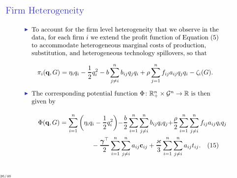
Firm Heterogeneity

To account for the firm level heterogeneity that we observe in thedata, for each firm i we extend the profit function of Equation (5)to accommodate heterogeneous marginal costs of production,substitution, and heterogeneous technology spillovers, so that

πi(q, G) = ηiqi −1

2q2i − b

n∑

j 6=i

bijqjqi + ρ

n∑

j=1

fijaijqjqi − ζi(G).

The corresponding potential function Φ: Rn+ × Gn → R is thengiven by

Φ(q, G) =n∑

i=1

(

ηiqi −1

2q2i

)

−b

2

n∑

i=1

n∑

j 6=i

bijqiqj+ρ

2

n∑

i=1

n∑

j 6=i

fijaijqiqj

−γ⊤

2

n∑

i=1

n∑

j 6=i

aijcij +κ

3

n∑

i=1

n∑

j 6=i

aijtij . (15)

26/46

Estimation Algorithms

The theoretical characterization of the stationary states via a Gibbsmeasure allows us to estimate the model’s parameters using threealternative estimation algorithms:

(i) a classical maximum likelihood method (MLE),

(ii) a double Metropolis-Hastings Markov Chain (DMH) Monte Carloalgorithm, which, differently to the MLE, allows for triadic termsin the cost function,

(iii) or an adaptive exchange algorithm (AEX), which overcomes theuncertainty of slow mixing faced by the DMH algorithm.25

25The AEX applies importance sampling to prevent the “local trap problem” (i.e. thesampler can escape local maxima of the potential function).

27/46

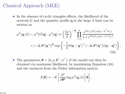
Classical Approach (MLE)

In the absence of cyclic triangles effects, the likelihood of thenetwork G and the quantity profile q in the large ϑ limit can bewritten as

µϑ(q, G) = µϑ(G|q) · µϑ(q) ≈

(2π

ϑ

)−n2

n∏

i<j

eϑaij(ρfijqiqj−γ⊤cij)

1 + eϑ(ρfijqiqj−γ⊤cij)

× |−∆H (q∗)|12 exp

−1

2ϑ(q − q∗)⊤(−∆H (q∗))(q− q∗)

,

(16)

The parameters θ = (b, ρ, δ⊤,γ⊤) of the model can then beobtained via maximum likelihood, by maximizing Equation (16),and the variances from the Fisher information matrix:

I(θ) = −E

[∂2

∂θ2logµϑ(q, G)

∣∣∣∣θ

]

,

28/46

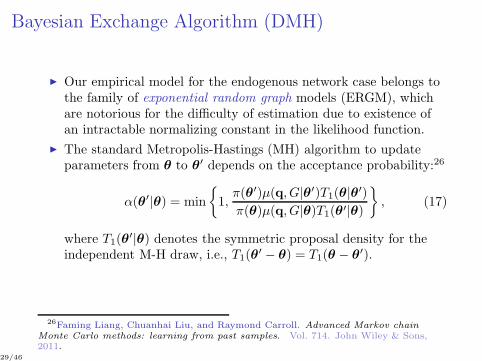
Bayesian Exchange Algorithm (DMH)

Our empirical model for the endogenous network case belongs tothe family of exponential random graph models (ERGM), whichare notorious for the difficulty of estimation due to existence ofan intractable normalizing constant in the likelihood function.

The standard Metropolis-Hastings (MH) algorithm to updateparameters from θ to θ′ depends on the acceptance probability:26

α(θ′|θ) = min

1,π(θ′)µ(q, G|θ′)T1(θ|θ′)

π(θ)µ(q, G|θ)T1(θ′|θ)

, (17)

where T1(θ′|θ) denotes the symmetric proposal density for the

independent M-H draw, i.e., T1(θ′ − θ) = T1(θ − θ′).

26Faming Liang, Chuanhai Liu, and Raymond Carroll. Advanced Markov chainMonte Carlo methods: learning from past samples. Vol. 714. John Wiley & Sons,2011.

29/46

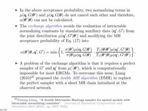
In the above acceptance probability, two normalizing terms inµ(q, G|θ′) and µ(q, G|θ) do not cancel each other and therefore,α(θ′|θ) can not be calculated.

The exchange algorithm avoids the evaluation of intractablenormalizing constants by simulating auxiliary data (q′, G′) fromthe joint distribution µ(q′, G′|θ′) and modifying the MHacceptance probability of Eq. (17) into

α(θ′|θ,q′, G′) = min

1,π(θ′)µ(q, G|θ′)

π(θ)µ(q, G|θ)·T1(θ|θ

′)µ(q′, G′|θ)

T1(θ′|θ)µ(q′, G′|θ′)

.

A problem of the exchange algorithm is that it requires a perfectsampler of G′ and q′ from µ(·|θ′), which is computationallyimpossible for most ERGMs. To overcome this issue, Liang(2010)27 proposed the double MH algorithm (DMH) to replacethe perfect sampler with a short MH chain initialized at theobserved network.

27Faming Liang. “A double Metropolis–Hastings sampler for spatial models withintractable normalizing constants”. Journal of Statistical Computation andSimulation 80.9 (2010), pp. 1007–1022.

30/46

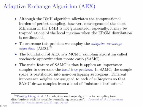
Adaptive Exchange Algorithm (AEX)

Although the DMH algorithm alleviates the computationalburden of perfect sampling, however, convergence of the shortMH chain in the DMH is not guaranteed, especially, it may betrapped at one of the local maxima when the ERGM distributionis mutlimodal.

To overcome this problem we employ the adaptive exchange

algorithm (AEX).28

The foundation of AEX is a MCMC sampling algorithm calledstochastic approximation monte carlo (SAMC).

The main feature of SAMC is that it applies an importancesampler to overcome the local trap problem. In SAMC, the samplespace is partitioned into non-overlapping subregions. Differentimportance weights are assigned to each of subregions so thatSAMC draws samples from a kind of “mixture distribution.”

28Faming Liang et al. “An adaptive exchange algorithm for sampling fromdistributions with intractable normalizing constants”. Journal of the AmericanStatistical Association (2015), pp. 00–00.

31/46

Table: Estimation results with homogeneous spillovers.

ExogenousMLE DMH

Network

ρ 0.0666∗∗∗ 0.0612∗∗∗ 0.0733∗∗∗ 0.0692∗∗∗

(0.0042) (0.0048) (0.0039) (0.0047)b 0.0008∗∗∗ 0.0005∗∗∗ 0.0009∗∗∗ 0.0008∗∗∗

(0.0001) (0.0001) (0.0002) (0.0002)Prod. 0.4936∗∗∗ 0.5576∗∗∗ 0.4761∗∗∗ 0.4789∗∗∗

(0.0462) (0.0544) (0.0459) (0.0658)

Cost function

Constant - -12.2102∗∗∗ -12.5871∗∗∗ -12.3511∗∗∗

- (0.4752) (0.7981) (1.2983)Same Sector - 2.4410∗∗∗ 2.4242∗∗∗ 2.5532∗∗∗

- (0.2567) -(0.4462) (0.6537)Same Country - 0.5184∗∗∗ 0.5836 0.2405

- (0.1717) (0.3329) (0.4094)Diff-in-Prod. - 1.2353∗∗∗ 1.4634∗∗ 1.6473∗∗

- (0.2995) (0.5818) (0.861)Diff-in-Prod. Sq. - -0.3072∗∗∗ -0.4087∗∗ -0.4751∗∗

- (0.087) (0.1721) (0.2639)Patents - 0.1809∗∗∗ 0.1724∗∗∗ 0.1434∗∗∗

- (0.0308) (0.0482) (0.0602)Cyclic Effect - - - 1.8806∗∗∗

- - - (0.4803)

Sector FE Yes Yes Yes Yes

Note: The estimation results are based on 351 firms from the SIC-28 sector. Theestimates reported are the posterior mean and posterior standard deviation (inparenthesis) from 50, 000 MCMC draws. The asterisks ∗∗∗(∗∗,∗) indicate thatits 99% (95%, 90%) highest posterior density range does not cover zero.

32/46

Policy Analysis

With our estimates from the previous section we are now able toperform various counterfactual policy studies:

(i) The first studies the impact on welfare of exit of a firm from thenetwork.

(ii) The second analyzes the welfare impact of a merger betweenfirms in the same sector.

(iii) The third policy intervention studies the welfare impact of asubsidy on the collaboration costs between pairs of firms, andaims at identifying the pair for which the subsidy yields thehighest welfare gains.

33/46

Firm Exit and Key Players

Table: Key player ranking for the chemicals and allied products sector with SIC code 28.

Firm Mkt. Sh. [%]a Patents Degree ∆W [%]b ∆WF [%]c ∆WN [%]d SIC Rank

Pfizer Inc. 2.7679 7844 15 -9.3298 -8.3045 -0.8576 283 1Novartis 2.0690 18924 15 -8.8432 -8.3180 -0.7028 283 2Amgen 0.8190 1885 13 -7.2453 -6.6007 -0.8979 283 3Bayer 3.8340 133433 10 -7.2364 -6.6212 -0.7721 280 4Merck & Co. Inc. 1.2998 52847 10 -5.8206 -4.3798 -0.8091 283 5Medarex Inc. 0.0028 168 9 -5.8066 -4.4589 -0.6733 283 6Exelixis 0.0056 283 7 -4.5366 -3.6320 -0.9021 283 7Xoma 0.0017 648 7 -4.2508 -3.2874 -0.6676 283 8Takeda Pharm. Co. Ltd. 0.6444 19460 7 -4.2237 -3.2980 -1.0186 283 9Daiichi Sankyo Co. Ltd. 0.4589 585 5 -4.1757 -3.0476 -0.8889 283 10Johnson & Johnson Inc. 3.0540 1212 7 -3.8065 -3.2701 -0.8189 283 11Bristol-Myers Squibb Co. 1.0287 6308 6 -3.6630 -3.2622 -0.8864 283 12Infinity Pharm. Inc. 0.0010 44 4 -3.6384 -2.3588 -0.5220 283 13Cell Genesys Inc. 0.0001 236 5 -3.4823 -1.9466 -0.4028 283 14Clinical Data Inc. 0.0036 6 4 -3.3530 -2.1821 -0.5455 283 15Compugen Ltd. 0.0001 22 5 -3.3255 -2.3133 -0.5922 283 16Dyax Corp. 0.0007 227 6 -3.1594 -2.4439 -0.5451 283 17MorphoSys AG 0.0038 20 4 -3.0709 -2.0938 -0.5237 283 18Seattle Genetics Inc. 0.0006 28 3 -2.6998 -1.2876 -0.5150 283 19Avalon Pharm. Inc. 0.0002 27 3 -2.6693 -1.2833 -0.5503 283 20

a Market share in the primary 3-digit sector in which the firm is operating.b The relative welfare loss due to exit of a firm i is computed as ∆W =(

E[W−i(G,q)] −W (qobs, Gobs))

/W (qobs, Gobs), where qobs and Gobs denote the observed R&D expenditures and

network, respectively.c ∆WF denotes the relative welfare loss due to exit of a firm assuming a fixed network G of R&D collaborations.d ∆WN denotes the relative welfare loss due to exit of a firm in the absence of a network G of R&D collaborations.

34/46

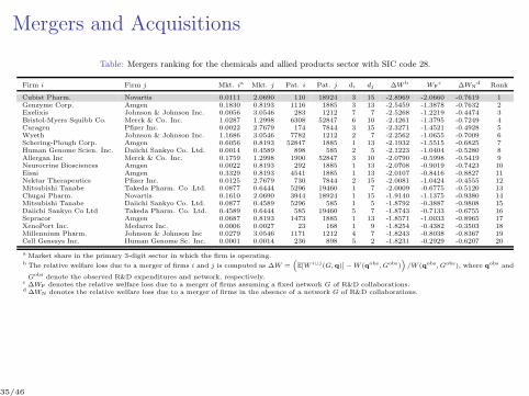
Mergers and Acquisitions

Table: Mergers ranking for the chemicals and allied products sector with SIC code 28.

Firm i Firm j Mkt. ia Mkt. j Pat. i Pat. j di dj ∆Wb WFc ∆WN

d Rank

Cubist Pharm. Novartis 0.0111 2.0690 110 18924 3 15 -2.8969 -2.0660 -0.7619 1Genzyme Corp. Amgen 0.1830 0.8193 1116 1885 3 13 -2.5459 -1.3878 -0.7632 2Exelixis Johnson & Johnson Inc. 0.0056 3.0546 283 1212 7 7 -2.5268 -1.2219 -0.4474 3Bristol-Myers Squibb Co. Merck & Co. Inc. 1.0287 1.2998 6308 52847 6 10 -2.4261 -1.3795 -0.7249 4Curagen Pfizer Inc. 0.0022 2.7679 174 7844 3 15 -2.3271 -1.4521 -0.4928 5Wyeth Johnson & Johnson Inc. 1.1686 3.0546 7782 1212 2 7 -2.2562 -1.0655 -0.7009 6Schering-Plough Corp. Amgen 0.6056 0.8193 52847 1885 1 13 -2.1932 -1.5515 -0.6825 7Human Genome Scien. Inc. Daiichi Sankyo Co. Ltd. 0.0014 0.4589 898 585 2 5 -2.1223 -1.0404 -0.5280 8Allergan Inc Merck & Co. Inc. 0.1759 1.2998 1900 52847 3 10 -2.0790 -0.5998 -0.5419 9Neurocrine Biosciences Amgen 0.0022 0.8193 292 1885 1 13 -2.0708 -0.9019 -0.7423 10Eisai Amgen 0.3329 0.8193 4541 1885 1 13 -2.0107 -0.8416 -0.8827 11Nektar Therapeutics Pfizer Inc. 0.0125 2.7679 730 7844 2 15 -2.0081 -1.0424 -0.4555 12Mitsubishi Tanabe Takeda Pharm. Co .Ltd. 0.0877 0.6444 5296 19460 1 7 -2.0009 -0.6775 -0.5120 13Chugai Pharm. Novartis 0.1610 2.0690 3944 18924 1 15 -1.9140 -1.1375 -0.9380 14Mitsubishi Tanabe Daiichi Sankyo Co. Ltd. 0.0877 0.4589 5296 585 1 5 -1.8792 -0.3887 -0.9808 15Daiichi Sankyo Co Ltd Takeda Pharm. Co. Ltd. 0.4589 0.6444 585 19460 5 7 -1.8743 -0.7133 -0.6755 16Sepracor Amgen 0.0687 0.8193 1473 1885 1 13 -1.8571 -1.0033 -0.8965 17XenoPort Inc. Medarex Inc. 0.0006 0.0027 23 168 1 9 -1.8254 -0.4382 -0.3503 18Millennium Pharm. Johnson & Johnson Inc 0.0279 3.0546 1171 1212 4 7 -1.8243 -0.8038 -0.8367 19Cell Genesys Inc. Human Genome Sc. Inc. 0.0001 0.0014 236 898 5 2 -1.8231 -0.2929 -0.6207 20

a Market share in the primary 3-digit sector in which the firm is operating.b The relative welfare loss due to a merger of firms i and j is computed as ∆W =

(

E[W i∪j(G,q)] −W (qobs, Gobs))

/W (qobs, Gobs), where qobs and

Gobs denote the observed R&D expenditures and network, respectively.c ∆WF denotes the relative welfare loss due to a merger of firms assuming a fixed network G of R&D collaborations.d ∆WN denotes the relative welfare loss due to a merger of firms in the absence of a network G of R&D collaborations.

35/46

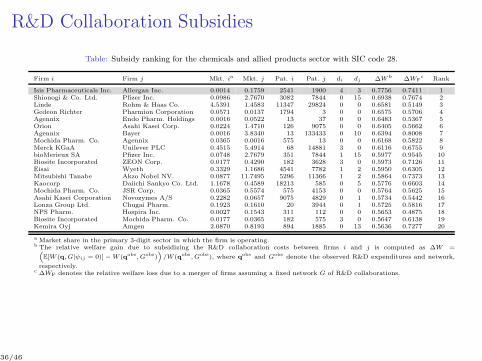
R&D Collaboration Subsidies

Table: Subsidy ranking for the chemicals and allied products sector with SIC code 28.

Firm i Firm j Mkt. ia Mkt. j Pat. i Pat. j di dj ∆Wb ∆WFc Rank

Isis Pharmaceuticals Inc. Allergan Inc. 0.0014 0.1759 2541 1900 4 3 0.7756 0.7411 1Shionogi & Co. Ltd. Pfizer Inc. 0.0986 2.7670 3082 7844 0 15 0.6938 0.7674 2Linde Rohm & Haas Co. 4.5391 1.4583 11347 29824 0 0 0.6581 0.5149 3Gedeon Richter Pharmion Corporation 0.0571 0.0137 1794 3 0 0 0.6575 0.5706 4Agennix Endo Pharm. Holdings 0.0016 0.0522 13 37 0 0 0.6483 0.5367 5Orion Asahi Kasei Corp. 0.0224 1.4710 126 9075 0 0 0.6405 0.5662 6Agennix Bayer 0.0016 3.8340 13 133433 0 10 0.6394 0.8008 7Mochida Pharm. Co. Agennix 0.0365 0.0016 575 13 0 0 0.6168 0.5822 8Merck KGaA Unilever PLC 0.4515 5.4914 68 14881 3 0 0.6116 0.6755 9bioMerieux SA Pfizer Inc. 0.0748 2.7679 351 7844 1 15 0.5977 0.9545 10Biosite Incorporated ZEON Corp. 0.0177 0.4290 182 3628 3 0 0.5973 0.7126 11Eisai Wyeth 0.3329 1.1686 4541 7782 1 2 0.5950 0.6305 12Mitsubishi Tanabe Akzo Nobel NV. 0.0877 11.7495 5296 11366 1 2 0.5864 0.7373 13Kaocorp Daiichi Sankyo Co. Ltd. 1.1678 0.4589 18213 585 0 5 0.5776 0.6603 14Mochida Pharm. Co. JSR Corp. 0.0365 0.5574 575 4153 0 0 0.5764 0.5625 15Asahi Kasei Corporation Novozymes A/S 0.2282 0.0657 9075 4829 0 1 0.5734 0.5442 16Lonza Group Ltd. Chugai Pharm. 0.1923 0.1610 20 3944 0 1 0.5725 0.5816 17NPS Pharm. Hospira Inc. 0.0027 0.1543 311 112 0 0 0.5653 0.4875 18Biosite Incorporated Mochida Pharm. Co. 0.0177 0.0365 182 575 3 0 0.5647 0.6138 19Kemira Oyj Amgen 2.0870 0.8193 894 1885 0 13 0.5636 0.7277 20

a Market share in the primary 3-digit sector in which the firm is operating.b The relative welfare gain due to subsidizing the R&D collaboration costs between firms i and j is computed as ∆W =(

E[W (q, G|ψij = 0)] −W (qobs, Gobs))

/W (qobs, Gobs), where qobs and Gobs denote the observed R&D expenditures and network,

respectively.c ∆WF denotes the relative welfare loss due to a merger of firms assuming a fixed network G of R&D collaborations.

36/46

Conclusion

We analyze the coevolution of networks and behavior, provide acomplete equilibrium characterization and show that our modelcan reproduce the observed patterns in real world networks.

The model can be conveniently estimated using state of the artBayesian algorithms, and (without triadic cost terms) can beestimated for arbitrarily large networks.

The model is amenable to policy analysis, and we illustrate thiswith examples for firm exit, M&As and subsidies in the contextof R&D collaboration networks.

Due to the generality of our payoff function the model can beapplied to a variety of related contexts such as peer effects ineducation, crime, risk sharing, financial contagion, scientificco-authorship, etc.29

Our methodology can also be applied to study discrete choice

models, and network games with local substitutes.

29Matthew O Jackson, Yves Zenou, et al. “Games on Networks”. Handbook ofGame Theory with Economic Applications 4 (2015), pp. 95–163.

37/46

Additional Results

38/46

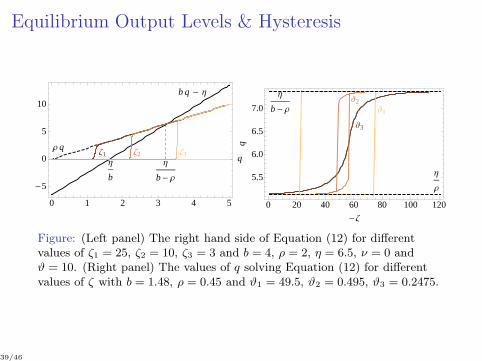
Equilibrium Output Levels & Hysteresis

b q - Η

Ρ q

Η

b

Η

b- Ρ

Ζ1 Ζ2 Ζ3

0 1 2 3 4 5

-5

0

5

10

q

Η

b- Ρ

Η

Ρ

J3

J2

J1

0 20 40 60 80 100 120

5.5

6.0

6.5

7.0

-Ζ

qFigure: (Left panel) The right hand side of Equation (12) for differentvalues of ζ1 = 25, ζ2 = 10, ζ3 = 3 and b = 4, ρ = 2, η = 6.5, ν = 0 andϑ = 10. (Right panel) The values of q solving Equation (12) for differentvalues of ζ with b = 1.48, ρ = 0.45 and ϑ1 = 49.5, ϑ2 = 0.495, ϑ3 = 0.2475.

39/46

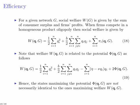
Efficiency

For a given network G, social welfare W (G) is given by the sumof consumer surplus and firms’ profits. When firms compete in ahomogeneous product oligopoly then social welfare is given by

W (q, G) =1

2

n∑

i=1

q2i +b

2

n∑

i=1

n∑

j 6=i

qiqj +

n∑

i=1

πi(q, G). (18)

Note that welfare W (q, G) is related to the potential Φ(q, G) asfollows

W (q, G) =1

2

n∑

i=1

q2i +b

2

n∑

i=1

n∑

j 6=i

qiqj −n∑

i=1

(η − νqi)qi + 2Φ(q, G).

(19)

Hence, the states maximizing the potential Φ(q, G) are not

necessarily identical to the ones maximizing welfare W (q, G).

40/46

Proposition: The efficient network G∗ ∈ Gn and output profileq∗ ∈ Qn are given by

(q∗, G∗) =

((η∗

b+2ν∗−ρ , . . .)

,Kn

)

, if ζ < ζ,((

η(n1−1)(b−ρ)+2ν−1 , . . . , 0, . . .

)

, Dn1,n−n1

)

, if ζ < ζ < ζ,((

η∗

b+2ν∗ , . . .)

,Kn

)

, if ζ < ζ,

(20)where η∗ = η/(n− 1), ν∗ = ν/(n− 1), ζ = ρ(η∗)2/(b+ 2ν∗)2,

ζ = ρ(η∗)2/(b+ 2ν∗ − ρ)2, Kn is the complete graph, Dn1,n−n1 is thedominant group architecture consisting of a clique of size n1 in whichall firms are connected and all remaining firms being isolated, Kn isthe empty graph, and n1 = argmaxk∈0,...,n W (k) with

W (k) =η2k(b(k − 1) + 2ν − 1)

2((b − ρ)(k − 1) + 2ν − 1)2− ζk(k − 1), (21)

with the property that n1 is increasing with decreasing ζ, b andincreasing with ρ and η.

41/46

Estimation for Exogenous Networks

A Laplace approximation30 (for large ϑ) of the Gibbs measureyields

µϑ(q, G) ≈

(2π

ϑ

)−n2

|−∇Φ(q∗, G)|12 e−

12ϑ(q−q

∗)⊤(−∆Φ(q∗,G))(q−q∗).

With the Hessian given by ∆Φ(q, G) = −M(G), q∗ = M(G)−1η,the matrix M(G) = M(G) ≡ In + bB− ρ(A F), and η = Xδ,the conditional density of output levels q given the (exogenous)network G can be rewritten as

µ(q, G) ≈

(2π

ϑ

)−n2

|M(G)|12 e−

12 (q−M(G)−1Xδ)

⊤M(G)(q−M(G)−1Xδ),

(22)which implies that the output q, conditional on the R&Dnetwork G, follows a Gaussian normal density function withmean M(G)−1Xδ and variance M(G)−1.

30R. Wong. Asymptotic approximations of integrals. Vol. 34. Society for IndustrialMathematics, 2001.

42/46

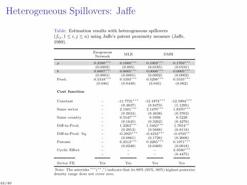
Heterogeneous Spillovers: Jaffe

Table: Estimation results with heterogeneous spillovers(fij , 1 ≤ i, j ≤ n) using Jaffe’s patent proximity measure (Jaffe,1989).

ExogenousMLE DMH

Network

ρ 0.2580∗∗∗ 0.1060∗∗∗ 0.1902∗∗∗ 0.1769∗∗∗

(0.0202) (0.005) (0.0185) (0.0191)b 0.0007∗∗∗ 0.0005∗∗∗ 0.0006∗∗∗ 0.0005∗∗∗

(0.0001) (0.0001) (0.0002) (0.0002)Prod. 0.5318∗∗∗ 0.5393∗∗∗ 0.5298∗∗∗ 0.5535∗∗∗

(0.046) (0.0448) (0.045) (0.062)

Cost function

Constant - -11.7721∗∗∗ -12.1874∗∗∗ -12.5904∗∗∗

- (0.4837) (0.8473) (1.1295)Same sector - 2.1501∗∗∗ 2.1470∗∗∗ 1.8270∗∗∗

- (0.2634) (0.4638) (0.3762)Same country - 0.5547∗∗∗ 0.5996 0.5228

- (0.1645) (0.3262) (0.4276)Diff-in-Prod. - 1.2262∗∗∗ 1.5463∗∗∗ 1.7654∗∗

- (0.2913) (0.5688) (0.8118)Diff-in-Prod. Sq. - -0.2925∗∗∗ -0.4233∗∗∗ -0.4705∗∗

- (0.0861) (0.1726) (0.2606)Patents - 0.2512∗∗∗ 0.2285∗∗∗ 0.1971∗∗∗

- (0.0248) (0.0469) (0.0818)Cyclic Effect - - - 3.3580∗∗∗

- - - (0.4475)

Sector FE Yes Yes Yes Yes

Note: The asterisks ∗∗∗(∗∗,∗) indicate that its 99% (95%, 90%) highest posteriordensity range does not cover zero.

43/46

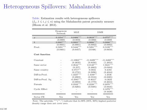
Heterogeneous Spillovers: Mahalanobis

Table: Estimation results with heterogeneous spillovers(fij , 1 ≤ i, j ≤ n) using the Mahalanobis patent proximity measure(Bloom et al. 2013).

ExogenousMLE DMH

Network

ρ 0.1054∗∗∗ 0.0406∗∗∗ 0.0818∗∗∗ 0.0757∗∗∗

(0.0085 (0.0056 (0.0066 (0.0095b 0.0007∗∗∗ 0.0005∗∗∗ 0.0006∗∗∗ 0.0006∗∗∗

(0.0001) (0.0001) (0.0002) (0.0002)Prod. 0.5291∗∗∗ 0.5444∗∗∗ 0.5291∗∗∗ 0.5199∗∗∗

(0.0461) (0.0457) (0.048) (0.0659)

Cost function

Constant - -11.8963∗∗∗ -11.8499∗∗∗ -11.6468∗∗∗

- (0.4635) (0.8456) (1.2653)Same sector - 2.2644∗∗∗ 2.0148∗∗∗ 1.9421∗∗∗

- (0.257) (0.4662) (0.6404)Same country - 0.5717∗∗ 0.5834 0.4183

- (0.1731) (0.3096) (0.4044)Diff-in-Prod. - 1.2237∗∗∗ 1.4160∗∗ 1.2536

- (0.2903) (0.5516) (0.8385)Diff-in-Prod. Sq. - -0.2945∗∗∗ -0.4013∗ -0.3622

- (0.0894) (0.1778) (0.2634)Patents - 0.2592∗∗∗ 0.2228∗∗∗ 0.2070∗∗∗

- (0.0265) (0.0495) (0.0645)Cyclic Effect - - - 3.1278∗∗∗

- - - (0.4428)

Sector FE Yes Yes Yes Yes

Note: The asterisks ∗∗∗(∗∗,∗) indicate that its 99% (95%, 90%) highest posteriordensity range does not cover zero.

44/46

Bayesian Identification

ρ

Density

−0.05 0.00 0.05 0.10 0.15 0.20 0.25

05

10

15

N=200

N=100

b

Density

0.00 0.01 0.02 0.03 0.04 0.05

020

40

60

80

N=200

N=100

ρ

Density

−0.05 0.00 0.05 0.10 0.15 0.20 0.25

05

10

15

N=200

N=100

b

Density

−0.04 −0.02 0.00 0.02 0.04 0.06

010

20

30

40

N=200

N=100

45/46

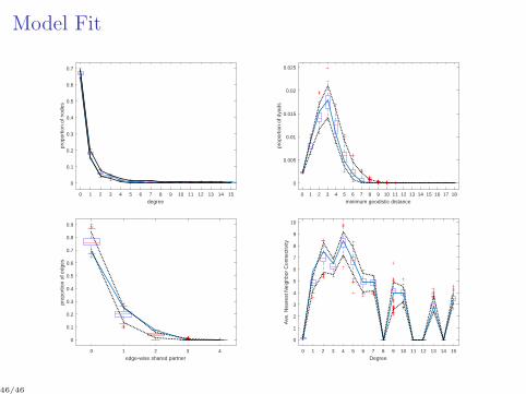
Model Fit

0 1 2 3 4 5 6 7 8 9 10 11 12 13 14 15

degree

0

0.1

0.2

0.3

0.4

0.5

0.6

0.7

prop

ortio

n of

nod

es

0 1 2 3 4 5 6 7 8 9 10 11 12 13 14 15 16 17 18

minimum geodistic distance

0

0.005

0.01

0.015

0.02

0.025

prop

ortio

n of

dya

ds

0 1 2 3 4

edge-wise shared partner

0

0.1

0.2

0.3

0.4

0.5

0.6

0.7

0.8

0.9

prop

ortio

n of

edg

es

0 1 2 3 4 5 6 7 8 9 10 11 12 13 14 15

Degree

0

1

2

3

4

5

6

7

8

9

10

Ave

. Nea

rest

Nei

ghbo

r C

onne

ctiv

ity

46/46