machine learning lecture regression basics...machine learning regression basics linear regression,...
TRANSCRIPT
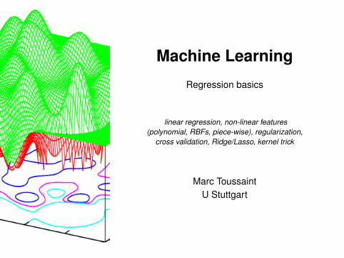
Machine Learning
Regression basics
linear regression, non-linear features(polynomial, RBFs, piece-wise), regularization,
cross validation, Ridge/Lasso, kernel trick
Marc ToussaintU Stuttgart
-1.5
-1
-0.5
0
0.5
1
1.5
-3 -2 -1 0 1 2 3
(MT/plot.h -> gnuplot pipe)
'train' us 1:2'model' us 1:2
-2
-1
0
1
2
3
-2 -1 0 1 2 3
(MT/plot.h -> gnuplot pipe)
traindecision boundary
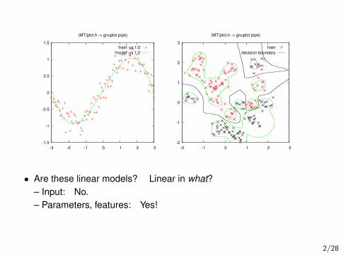
• Are these linear models? Linear in what?– Input: No.– Parameters, features: Yes!
2/28

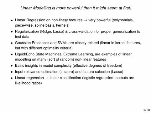
Linear Modelling is more powerful than it might seem at first!
• Linear Regression on non-linear features→ very powerful (polynomials,piece-wise, spline basis, kernels)
• Regularization (Ridge, Lasso) & cross-validation for proper generalization totest data
• Gaussian Processes and SVMs are closely related (linear in kernel features,but with different optimality criteria)
• Liquid/Echo State Machines, Extreme Learning, are examples of linearmodelling on many (sort of random) non-linear features
• Basic insights in model complexity (effective degrees of freedom)
• Input relevance estimation (z-score) and feature selection (Lasso)
• Linear regression→ linear classification (logistic regression: outputs arelikelihood ratios)
⇒ Good foundation for learning about ML(We roughly follow Hastie, Tibshirani, Friedman: Elements of Statistical
Learning)
3/28

Linear Modelling is more powerful than it might seem at first!
• Linear Regression on non-linear features→ very powerful (polynomials,piece-wise, spline basis, kernels)
• Regularization (Ridge, Lasso) & cross-validation for proper generalization totest data
• Gaussian Processes and SVMs are closely related (linear in kernel features,but with different optimality criteria)
• Liquid/Echo State Machines, Extreme Learning, are examples of linearmodelling on many (sort of random) non-linear features
• Basic insights in model complexity (effective degrees of freedom)
• Input relevance estimation (z-score) and feature selection (Lasso)
• Linear regression→ linear classification (logistic regression: outputs arelikelihood ratios)
⇒ Good foundation for learning about ML(We roughly follow Hastie, Tibshirani, Friedman: Elements of Statistical
Learning)3/28

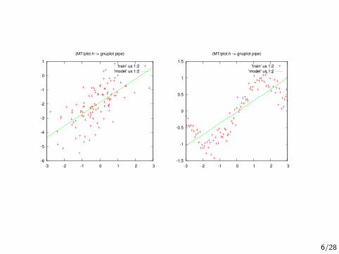
Linear Regression
• Notation:– input vector x ∈ Rd
– output value y ∈ R– parameters β = (β0, β1, .., βd)
>∈ Rd+1
– linear model
f(x) = β0 +∑dj=1 βjxj
• Given training data D = {(xi, yi)}ni=1 we define the least squares cost(or “loss”)
Lls(β) =∑ni=1(yi − f(xi))2
4/28

Linear Regression
• Notation:– input vector x ∈ Rd
– output value y ∈ R– parameters β = (β0, β1, .., βd)
>∈ Rd+1
– linear model
f(x) = β0 +∑dj=1 βjxj
• Given training data D = {(xi, yi)}ni=1 we define the least squares cost(or “loss”)
Lls(β) =∑ni=1(yi − f(xi))2
4/28

Optimal parameters β
• Augment input vector with a 1 in front:x = (1, x) = (1, x1, .., xd)
>∈ Rd+1
β = (β0, β1, .., βd)>∈ Rd+1
f(x) = β0 +∑nj=1 βjxj = x
>β
• Rewrite sum of squares as:Lls(β) =
∑ni=1(yi − x>iβ)2 = ||y −Xβ||2
X =
x>1...x>n
=
1 x1,1 x1,2 · · · x1,d...
...1 xn,1 xn,2 · · · xn,d
, y =
y1...yn
• Optimum:0>d =
∂Lls(β)∂β = −2(y −Xβ)>X ⇐⇒ 0d =X
>Xβ −X>y
β̂ ls = (X>X)-1X>y
5/28
-6
-5
-4
-3
-2
-1
0
1
-3 -2 -1 0 1 2 3
(MT/plot.h -> gnuplot pipe)
'train' us 1:2'model' us 1:2
-1.5
-1
-0.5
0
0.5
1
1.5
-3 -2 -1 0 1 2 3
(MT/plot.h -> gnuplot pipe)
'train' us 1:2'model' us 1:2
6/28

Non-linear features
• Replace the inputs xi ∈ Rd by some non-linear features φ(xi) ∈ Rk
f(x) =∑kj=1 φj(x) βj = φ(x)>β
• The optimal β is the same
β̂ ls = (X>X)-1X>y but with X =
φ(x1)>
...φ(xn)
>
∈ Rn×k
• What are “features”?a) Features are an arbitrary set of basis functionsb) Any function linear in β can be written as f(x) = φ(x)>β
for some φ – which we denote as “features”
7/28
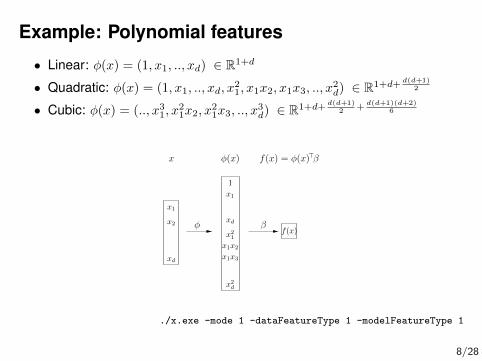
Example: Polynomial features
• Linear: φ(x) = (1, x1, .., xd) ∈ R1+d
• Quadratic: φ(x) = (1, x1, .., xd, x21, x1x2, x1x3, .., x
2d) ∈ R1+d+
d(d+1)2
• Cubic: φ(x) = (.., x31, x21x2, x
21x3, .., x
3d) ∈ R1+d+
d(d+1)2 +
d(d+1)(d+2)6
x1
x2
xd
φ β
1
x21
x1
xd
x1x2
x1x3
x2d
φ(x)x f(x) = φ(x)>β
f(x)
./x.exe -mode 1 -dataFeatureType 1 -modelFeatureType 1
8/28

Example: Piece-wise features
• Piece-wise constant: φj(x) = I(ξ1 < x < ξ2)
• Piece-wise linear: φj(x) = xI(ξ1 < x < ξ2)
• Continuous piece-wise linear: φj(x) = (x− ξ1)+
9/28
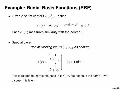
Example: Radial Basis Functions (RBF)
• Given a set of centers {cj}kj=1, define
φj(x) = b(x, cj) = e−12 ||x−cj ||
2
∈ [0, 1]
Each φj(x) measures similarity with the center cj
• Special case:use all training inputs {xi}ni=1 as centers
φ(x) =
1
b(x, x1)...
b(x, xn)
(n+ 1 dim)
This is related to “kernel methods” and GPs, but not quite the same – we’ll
discuss this later.
10/28

Features
• Polynomial
• Piece-wise
• Radial basis functions (RBF)
• Splines (see Hastie Ch. 5)
• Linear regression on top of rich features is extremely powerful!
11/28

The need for regularizationNoisy sin data fitted with radial basis functions
-1.5
-1
-0.5
0
0.5
1
1.5
2
-3 -2 -1 0 1 2 3
(MT/plot.h -> gnuplot pipe)
'z.train' us 1:2'z.model' us 1:2
./x.exe -mode 1 -n 40 -modelFeatureType 4 -dataType 2 -sigma .3 -lambda
1e-10
• Overfitting & generalization:The model overfits to the data – and generalizes badly
• Estimator variance:When you repeat the experiment (keeping the underlying functionfixed), the regression always returns a different model estimate
12/28
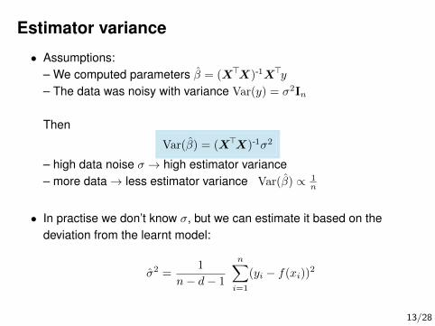
Estimator variance
• Assumptions:– We computed parameters β̂ = (X>X)-1X>y
– The data was noisy with variance Var(y) = σ2In
Then
Var(β̂) = (X>X)-1σ2
– high data noise σ → high estimator variance– more data→ less estimator variance Var(β̂) ∝ 1
n
• In practise we don’t know σ, but we can estimate it based on thedeviation from the learnt model:
σ̂2 =1
n− d− 1
n∑i=1
(yi − f(xi))2
13/28

Estimator variance
• “Overfitting”← picking one specific data set y ∼ N(ymean, σ
2In)
↔ picking one specific b̂ ∼ N(βmean, (X>X)-1σ2)
• If we could reduce the variance of the estimator, we could reduceoverfitting – and increase generalization.
14/28
Hastie’s section on shrinkage methods is great! Describes severalideas on reducing estimator variance — by reducing model complexity.We focus on regularization.
15/28
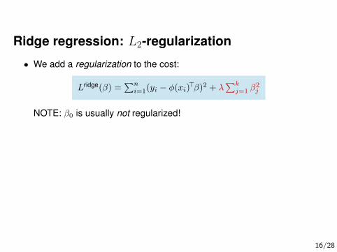
Ridge regression: L2-regularization
• We add a regularization to the cost:
Lridge(β) =∑ni=1(yi − φ(xi)>β)2 + λ
∑kj=1 β
2j
NOTE: β0 is usually not regularized!
• Optimum:
β̂ridge = (X>X + λI)-1X>y
(where I = Ik, or with I1,1 = 0 if β0 is not regularized)
16/28

Ridge regression: L2-regularization
• We add a regularization to the cost:
Lridge(β) =∑ni=1(yi − φ(xi)>β)2 + λ
∑kj=1 β
2j
NOTE: β0 is usually not regularized!
• Optimum:
β̂ridge = (X>X + λI)-1X>y
(where I = Ik, or with I1,1 = 0 if β0 is not regularized)
16/28
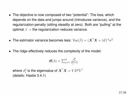
• The objective is now composed of two “potential”: The loss, whichdepends on the data and jumps around (introduces variance), and theregularization penalty (sitting steadily at zero). Both are “pulling” at theoptimal β → the regularization reduces variance.
• The estimator variance becomes less: Var(β̂) = (X>X + λI)-1σ2
• The ridge effectively reduces the complexity of the model:
df(λ) =∑dj=1
d2jd2j+λ
where d2j is the eigenvalue of X>X = V D2V>
(details: Hastie 3.4.1)
17/28

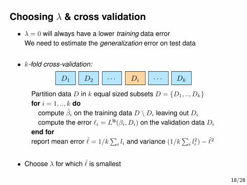
Choosing λ & cross validation
• λ = 0 will always have a lower training data errorWe need to estimate the generalization error on test data
• k-fold cross-validation:
D1 D2 Di Dk· · · · · ·
Partition data D in k equal sized subsets D = {D1, .., Dk}for i = 1, .., k do
compute β̂i on the training data D \Di leaving out Di
compute the error `i = Lls(βi, Di) on the validation data Di
end forreport mean error ˆ̀= 1/k
∑i li and variance (1/k
∑i l
2i )− ˆ̀2
• Choose λ for which ˆ̀ is smallest
18/28

quadratic features on sinus data:
0.4
0.5
0.6
0.7
0.8
0.9
1
1.1
1.2
1.3
0.001 0.01 0.1 1 10 100 1000 10000 100000
mean s
quare
d e
rror
lambda
(MT/plot.h -> gnuplot pipe)
cv errortraining error
./x.exe -mode 4 -n 10 -modelFeatureType 2 -dataType 2 -sigma .1
./x.exe -mode 1 -n 10 -modelFeatureType 2 -dataType 2 -sigma .1
19/28
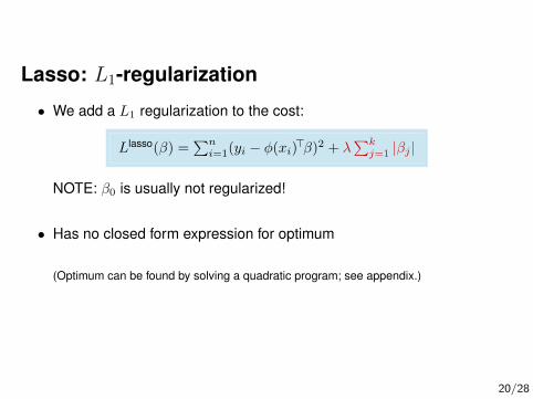
Lasso: L1-regularization
• We add a L1 regularization to the cost:
Llasso(β) =∑ni=1(yi − φ(xi)>β)2 + λ
∑kj=1 |βj |
NOTE: β0 is usually not regularized!
• Has no closed form expression for optimum
(Optimum can be found by solving a quadratic program; see appendix.)
20/28

Lasso vs. Ridge:
• Lasso→ sparsity! feature selection!
21/28

Lq(β) =∑ni=1(yi − φ(xi)>β)2 + λ
∑kj=1 |βj |q
• Subset selection: q = 0 (counting the number of βj 6= 0)
22/28

Summary
• Linear models on non-linear features – extremely powerful
linearpolynomial
RBFkernel
RidgeLasso
regressionclassification
• Generalization ↔ Regularization ↔ complexity/DoF penalty
• Cross validation to estimate generalization empirically→ use tochoose regularization parameters
23/28

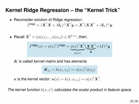
Kernel Ridge Regression – the “Kernel Trick”
• Reconsider solution of Ridge regression:β̂ridge = (X>X + λIk)
-1X>y =X>(XX>+ λIn)-1y
• Recall X>= (φ(x1), .., φ(xn)) ∈ Rk×n, then:
f ridge(x) = φ(x)>βridge = φ(x)>X>︸ ︷︷ ︸κ(x)
(XX>︸ ︷︷ ︸K
+λI)-1y
K is called kernel matrix and has elements
Kij = k(xi, xj) := φ(xi)>φ(xj)
κ is the kernel vector: κ(x) = k(x, x1:n) = φ(x)>X>.
The kernel function k(x, x′) calculates the scalar product in feature space.
24/28
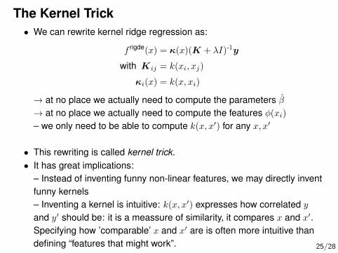
The Kernel Trick• We can rewrite kernel ridge regression as:
f rigde(x) = κ(x)(K + λI)-1y
with Kij = k(xi, xj)
κi(x) = k(x, xi)
→ at no place we actually need to compute the parameters β̂→ at no place we actually need to compute the features φ(xi)– we only need to be able to compute k(x, x′) for any x, x′
• This rewriting is called kernel trick.• It has great implications:
– Instead of inventing funny non-linear features, we may directly inventfunny kernels– Inventing a kernel is intuitive: k(x, x′) expresses how correlated yand y′ should be: it is a meassure of similarity, it compares x and x′.Specifying how ’comparable’ x and x′ are is often more intuitive thandefining “features that might work”. 25/28

• Every choice of features implies a kernel. But,Does every choice of kernel correspond to specific choice of feature?
26/28

Reproducing Kernel Hilbert Space• Let’s define a vector space Hk, spanned by infinitely many basis elements
{hx = k(·, x) : x ∈ Rd}
Vectors in this space are linear combinations of such basis elements, e.g.,
f =∑i
αihxi , f(x) =∑i
αik(x, xi)
• Let’s define a scalar product in this space, by first defining the scalar productfor every basis element,
〈hx, hy〉 := k(x, y)
This is positive definite. Note, it follows
〈hx, f〉 =∑i
αi 〈hx, hxi〉 =∑i
αik(x, xi) = f(x)
• The φ(x) = hx = k(·, x) is the ‘feature’ we associate with x. Note that this is afunction and infinite dimensional.Choosing α = (K + λI)-1y represents f ridge(x) =
∑ni=1 αik(x, xi), and shows
that ridge regression has a finite-dimensional solution in the basis elements{hxi}. A much more general version of this insight is called representertheorem. 27/28

Example Kernels
• Kernel functions need to be positive definite: ∀z:|z|>0 : k(z, z′) > 0
→K is a positive definite matrix
• Examples:– Polynomial: k(x, x′) = (x>x′)d
d = 2, x ∈ R2, φ(x) =(x21,√2x1x2, x
22
)>
k(x, x′) = ((x1, x2)
x′1
x′2
)2
= (x1x′1 + x2x
′2)
2
= x21x′12+ 2x1x2x
′1x′2 + x22x
′22
= (x21,√2x1x2, x
22)(x
′12,√2x′1x
′2, x′22)>
= φ(x)>φ(x′)
– Gaussian (radial basis function): k(x, x′) = exp(−γ |x− x′ | 2)
28/28

Appendix: Alternative formulation of Ridge
• The standard way to write the Ridge regularization:Lridge(β) =
∑ni=1(yi − φ(xi)>β)2 + λ
∑kj=1 β
2j
• Finding β̂ridge = argminβ Lridge(β) is equivalent to solving
β̂ridge = argminβ
n∑i=1
(yi − φ(xi)>β)2
subject tok∑j=1
β2j ≤ t
λ is the Karush-Kuhn-Tucker multiplier for the inequality constraint(generalization of Lagrange multiplier)
29/28
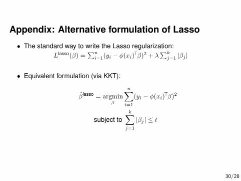
Appendix: Alternative formulation of Lasso
• The standard way to write the Lasso regularization:Llasso(β) =
∑ni=1(yi − φ(xi)>β)2 + λ
∑kj=1 |βj |
• Equivalent formulation (via KKT):
β̂ lasso = argminβ
n∑i=1
(yi − φ(xi)>β)2
subject tok∑j=1
|βj | ≤ t
30/28