the algebra of linear regression - statpower.net notes/regressionalgebra.pdf · the algebra of...

The Algebra of Linear Regression

James H. Steiger

Department of Psychology and Human DevelopmentVanderbilt University

James H. Steiger (Vanderbilt University) The Algebra of Linear Regression 1 / 30

The Algebra of Linear Regression1 Introduction

2 Bivariate Linear Regression

3 Multiple Linear Regression

4 Multivariate Linear Regression

5 Extensions to Random Variables and Random Vectors

6 Partial Correlation


Introduction

Introduction

In this module, we explore the algebra of least squares linear regression systems with aspecial eye toward developing the properties useful for deriving factor analysis andstructural equation modeling.A key insight is that important properties hold whether or not variables are observed.


Bivariate Linear Regression


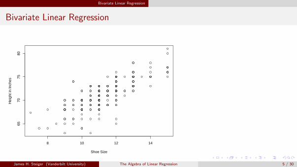
In bivariate linear regression performed on a sample of n observations, we seek to examinethe extent of the linear relationship between two observed variables, X and Y .One variable (usually the one labeled Y ) is the dependent or criterion variable, the other(usually labeled X ) is the independent or predictor variable.Each data point represents a pair of scores, xi , yi that may be plotted as a point in theplane. Such a plot, called a scatterplot, is shown on the next slide.In these data, gathered on a group of male college students, the independent variableplotted on the horizontal (X ) axis is shoe size, and the dependent variable plotted on thevertical (Y ) axis is height in inches.




8 10 12 14

6570

7580

Shoe Size

Hei

ght i

n In

ches




It would be a rare event, indeed, if all the points fell on a straight line. However, if Y andX have an approximate linear relationship, then a straight line, properly placed, shouldfall close to many of the points.Choosing a straight line involves choosing the slope and intercept, since these twoparameters define any straight line.The regression model in the sample is that

yi = β0 + β1xi + ei (1)

Generally, the least squares criterion, minimizing∑n

i=1 e2i under choice of β0 and β1, is

employed.Minimizing

∑ni=1 e

2i is accomplished with the following well-known least squares solution.

β1 =rY ,XSYSX

=sY ,Xs2X

= s−1X ,X sx ,y (2)

β0 = Y • − β1X • (3)



Bivariate Linear RegressionDeviation Score Formulas

Suppose we were to convert X into deviation score form. This would have no effect onany variance, covariance or correlation involving X , but would change the mean of X tozero.What would be the effect on the least squares regression?Defining x∗i = xi − X •, we have the new least squares setup

yi = β∗0 + β∗1x∗i + e∗i (4)

From the previous slide, we know that β∗1 = SY ,X∗/SX∗,X∗ = SY ,X/SX ,X = β1, and that

β∗0 = Y • − β∗1X∗• = Y •.

Thus, if X is shifted to deviation score form, the slope of the regression line remainsunchanged, but the intercept shifts to Y •.It is easy to see that, should we also re-express the Y variable in deviation score form, theregression line intercept will shift to zero and the slope will still remain unchanged.



Bivariate Linear RegressionVariance of Predicted Scores

Using linear transformation rules, one may derive expressions for the variance of thepredicted (yi ) scores, the residual (ei ) scores, and the covariance between them.For example consider the variance of the predicted scores. Remember that adding aconstant (in this case β0) has no effect on a variance, and multiplying by a constantmultiplies the variance by the square of the multiplier. So, since yi = β1xi + β0, it followsimmediately that

s2Y

= β21S2X

= (rY ,XSY /SX )2S2X

= r2Y ,XS2Y (5)



Bivariate Linear RegressionCovariance of Predicted and Criterion Scores

The covariance between the criterion scores (yi ) and predicted scores (yi ) is obtained bythe heuristic rule.Begin by re-expressing yi as β1xi + β0, then recall that additive constant β0 cannot affecta covariance.So the covariance between yi and yi is the same as the covariance between yi and β1xi .Using the heuristic approach, we find that SY ,Y = SY ,β1X = β1SY ,X Recalling that

SY ,X = rY ,XSY SX , and β1 = rY ,XSY /SX , one quickly arrives at

SY ,Y = β1SY ,X

= (rY ,XSY SX )(rY ,XSY /SX )

= r2Y ,XS2Y

= S2Y

(6)



Bivariate Linear RegressionCovariance of Predicted and Residual Scores

Calculation of the covariance between the predicted scores and residual scores proceeds inmuch the same way. Re-express ei as yi − yi , then use the heuristic rule. One obtains

SY ,E = SY ,Y−Y

= SY ,Y − S2Y

= S2Y− S2

Y(from Equation 6)

= 0 (7)



Bivariate Linear RegressionCovariance of Predicted and Residual Scores

Calculation of the covariance between the predicted scores and residual scores proceeds inmuch the same way.Re-express ei as yi − Yi , then use the heuristic rule. One obtains

SY ,E = SY ,y−Y

= SY ,y − S2Y

= S2Y− S2

Y(from Equation 6)

= 0 (8)

Predicted and error scores always have exactly zero covariance, and zero correlation, inlinear regression.



Bivariate Linear RegressionAdditivity of Variances

Linear regression partitions the variance of Y into non-overlapping portions.Using a similar approach to the previous proofs, we may show easily that

S2Y = S2

Y+ S2

E (9)


Multiple Linear Regression


Multiple linear regression with a single criterion variable and several predictors is astraightforward generalization of bivariatelinear regression.To make the notation simpler, assume that the criterion variable Y and the p predictorvariables Xj , j = 1, . . . , p are in deviation score form.Let y be an n × 1 vector of criterion scores, and X be the n × p matrix with the predictorvariables in columns. Then the multiple regression prediction equation in the sample is

y = y + e

= Xβ + e (10)




The least squares criterion remains essentially as before, i.e., minimize∑

e2i = e′e under

choice of β. The unique solution is

β =(X′X

)−1X′y (11)

which may also be written asβ = S−1XXSXY (12)


Multivariate Linear Regression


The notation for multiple linear regression with a single criterion generalizes immediatelyto situations where more than one criterion is being predicted simultaneously.Specifically, let n × q matrix Y contain q criterion variables, and let β be a p × q matrixof regression weights. The least squares criterion is satisfied when the sum of squarederrors across all variables (i.e. Tr(E′E)) is minimized.The unique solution is the obvious generalization of Equation 11, i.e.,

B =(X′X

)−1X′Y (13)




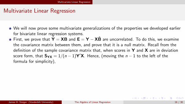
We will now prove some multivariate generalizations of the properties we developed earlierfor bivariate linear regression systems.First, we prove that Y = XB and E = Y − XB are uncorrelated. To do this, we examinethe covariance matrix between them, and prove that it is a null matrix. Recall from thedefinition of the sample covariance matrix that, when scores in Y and X are in deviationscore form, that SYX = 1/(n − 1)Y′X. Hence, (moving the n − 1 to the left of theformula for simplicity),




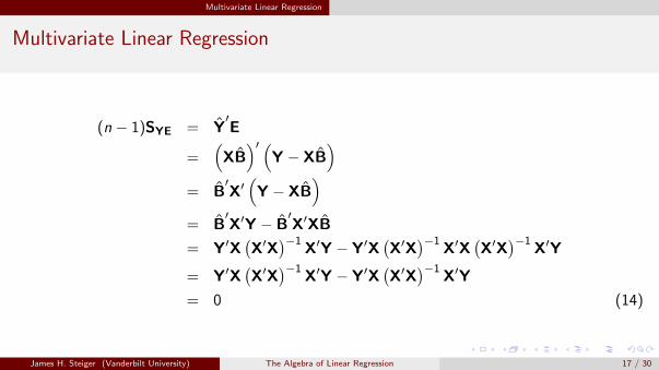
(n − 1)SYE = Y′E

=(XB)′ (

Y − XB)

= B′X′(Y − XB

)= B

′X′Y − B

′X′XB

= Y′X(X′X

)−1X′Y − Y′X

(X′X

)−1X′X

(X′X

)−1X′Y

= Y′X(X′X

)−1X′Y − Y′X

(X′X

)−1X′Y

= 0 (14)




The preceding result makes it easy to show that the variance-covariance matrix of Y isthe sum of the variance-covariance matrices for Y and E. Specifically,

(n − 1)SYY = Y′Y

=(Y + E

)′ (Y + E

)=

(Y′

+ E′)(

Y + E)

= Y′Y + E′Y + Y

′E + E′E

= Y′Y + 0 + 0 + E′E

= Y′Y + E′E




ConsequentlySYY = SYY + SEE (15)

Notice also thatSEE = SYY − B′SXXB (16)


Extensions to Random Variables and Random Vectors


In the previous section, we developed results for sample bivariate regression, multipleregression and multivariate regression.We saw that, in the sample, a least squares linear regression system is characterized byseveral key propertiesSimilar relationships hold when systems of random variables arerelated in a linear least-squares regression system.In this section, we extend these results to least-squares linear regression systems relatingrandom variables or random vectors.We will develop the results for the multivariate regression case, as these results includethe bivariate and multiple regression systems as special cases.




Suppose there are p criterion variables in the random vector y , and q predictor variablesin the random vector x. For simplicity, assume all variables have means of zero, so nointercept is necessary. The prediction equation is

y = B′x + e (17)

= y + e (18)

In the population, the least-squares solution also minimizes the average squared error, butin the long run sense of minimizing the expected value of the sum of squared errors, i.e.,Tr E (ee′).The solution for B is

B = Σ−1xx Σxy (19)

with Σxx = E (xx′) the variance-covariance matrix of the random variables in x, andΣxy = E (xy′) the covariance matrix between the random vectors x and y.




The covariance matrix between predicted and error variables is null, just as in the samplecase. The proof is structurally similar to its sample counterpart, but we include it here todemonstrate several frequently used techniques in the matrix algebra of expected values.

Σye = E(ye′)

= E(B′x(y − B′x)′

)= E

(ΣyxΣ

−1xx xy

′ − ΣyxΣ−1xx xx

′Σ−1xx Σyx

)= ΣyxΣ

−1xx E (xy′) − ΣyxΣ

−1xx E (xx′)Σ−1xx Σyx

= ΣyxΣ−1xx Σxy − ΣyxΣ

−1xx ΣxxΣ

−1xx Σyx

= ΣyxΣ−1xx Σxy − ΣyxΣ

−1xx Σyx

= 0 (20)




We also find thatΣyy = Σyy + Σee (21)

andΣee = Σyy − B′ΣxxB (22)

Consider an individual random variable yi in y. The correlation between yi and itsrespective yi is called “the multiple correlation of yi with the predictor variables in x.”Suppose that the variables in x were uncorrelated, and that they and the variables in yhave unit variances, so that Σxx = I, an identity matrix, and, as a consequence, B = Σxy.




Then the correlation between a particular yi and its respective yi is

ryi ,yi =σyi yi√σ2yiσ

2yi

=E(yi (b

′ix)′)√

(1)(b′iΣxxbi )

=E (yix

′bi )√(b′iΣxxbi )

=E (yix

′)bi√(b′iΣxxbi )

=σyixbi√(b′ibi )

=b′ibi√(b′ibi )

(23)




It follows immediately that, when the predictor variables in x are orthogonal with unitvariance, squared multiple correlations may be obtained directly as a sum of squared,standardized regression weights.In subsequent chapters, we will be concerned with two linear regression prediction systemsknown (loosely) as “factor analysis models,” but referred to more precisely as “commonfactor analysis” and “principal component analysis.”In each system, we will be attempting to reproduce an observed (or “manifest”) set of prandom variables in as (least squares) linear functions of a smaller set of m hypothetical(or “latent”) random variables.


Partial Correlation

Partial Correlation

In many situations, the correlation between two variables may be substantially differentfrom zero without implying any causal connection between them.A classic example is the high positive correlation between number of fire engines sent to afire and the damage done by the fire.Clearly, sending fire engines to a fire does not usually cause damage, and it is equallyclear that one would be ill-advised to recommend reducing the number of trucks sent to afire as a means of reducing damage.


Partial Correlation

Partial Correlation

In situations like the house fire example, one looks for (indeed often hypothesizes ontheoretical grounds) a “third variable” which is causally connected with the first twovariables, and “explains” the correlation between them.In the house fire example, such a third variable might be “size of fire.”One would expect that, if size of fire were held constant, there would be, if anything, anegative correlation between damage done by a fire and the number of fire engines sentto the fire.


Partial Correlation

Partial Correlation

One way of statistically holding the third variable “constant” is through partial correlationanalysis.In this analysis, we “partial out” the third variable from the first two by linear regression,leaving two linear regression error, or residual variables. We then compute the “partialcorrelation” between the first two variables as the correlation between the two regressionresiduals.A basic notion connected with partial correlation analysis is that, if, by partialling out oneor more variables, you cause the partial correlations among some (other) variables to goto zero, then you have “explained” the correlations among the (latter) variables as being“due to” the variables which were partialled out.


Partial Correlation

Partial Correlation

If, in terms of Equation 18 above, we “explain” the correlations in the variables in y bythe variables in x, then e should have a correlation (and covariance) matrix which isdiagonal, i.e., the variables in e should be uncorrelated once we “partial out” the variablesin x by linear regression.Recalling Equation ?? we see that this implies that Σyy − B′ΣxxB is a diagonal matrix.


Partial Correlation

Partial Correlation

This seemingly simple result has some rather surprisingly powerful ramifications, once onedrops certain restrictive mental sets.In subsequent lectures, we shall see how, at the turn of the 20th century, this result ledCharles Spearman to a revolutionary linear regression model for human intelligence, andan important new statistical technique for testing the model with data. What wassurprising about the model was that it could be tested, even though the predictorvariables (in x) are never directly observed!


the algebra of linear regression - statpower.net notes/regressionalgebra.pdf · the algebra of...

Documents