econometrics notes (introduction, simple linear regression, multiple linear regression)

Muhammad Ali Econometrics

Lecturer in Statistics GPGC Mardan. BS Economics

M.sc (Peshawar University)

Mphil(AIOU Islamabad)

1

Introduction

Definition of Econometrics

literally interpreted econometrics means "economic measurement". Econometrics may be defined as

the social science in which the tools of economic theory, mathematics, and statistical inference are

applied to the analysis of economic phenomena(variable).Econometrics can also be defined as

"statistical observation of theoretically formed concepts OR alternatively as mathematical economics

working with measured data. so economic theory attempts to defined the relationship among different

economic variables.

Methodology of Econometrics

Following are the main steps in methodology of econometrics

1. Specify mathematical equation to describe the relationship between economic variables.

2. Design methods and procedures based on statistical theory to obtain representative sample

from the real world.

3. Development of methods for estimating the parameters of the specified relationships

4. Development of methods of making economic forecast for policy implications based on

estimated parameters.





2

What are the goals of econometrics

Econometrics help us to achieves the following three goals:

1. Judge the validity of the economic theories.

2. Supply the numerical estimates of the co-efficient of the economic relationships which may be

then used for some sound economic policies.

3. Forecast the future values of the economic magnitude with certain degree of probability.

The Nature of Econometrics Approach

The first step of every econometrics research is the specification of the model, a model is simply a set of

mathematical equations. If the model has only one equation it is called a single-equation model.

Whereas if it has more than one equation it is called a multi-equation model. Now let us consider the

following model.

Y=β0 + β1X

where

Y= Consumption expenditure

β0 = Intercept

β1= Slope or co-efficient of regression

X= income

This is a deterministic model showing the relationship between consumption and income.

The non-deterministic or stochastic models can be written as:

Yi=β0 + β1X i+ iε





3

where " iε " is known as the disturbance or residual term, and hence it is a random variable. It is also

called probabilistic model. The disturbance or error term represent all those factors that affect

consumption but not taken into account. This equation is an example of an "Econometric Model".

In other words it is an example of a "linear regression Model". In this case the response variable 'Y' is

linearly related to the predictor variable 'X' but the relationship between the two is not exact. The

second step is the estimation of model by appropriate econometric method, this will include the

following steps.

1. Collection of Data for the variables included in the model.

2. Choice of appropriate econometric technique for the estimation of technique used is Regression

Analysis in Statistics).

3. The third step is to develop the suitable criteria to find out whether estimates obtained are

in agreement with the expectations of the theory that has been tested, that is to decide whether

the estimates of the parameters of the theoretically meaning full and statistically significant.

4. The final step is to use the estimated model to predict the future value of the response variable.

Deterministic and Stochastic Models

A relation between X and Y is said to be deterministic if for each value of predictor variable X,

there is one and only one corresponding values of response variable Y. On the other hand the

relation between X and Y is said to be stochastic or probabilistic if for a predictor value of X 4

there is a whole probability distribution of values of Y, that is 'Y' is a random variable and 'X' is a

fixed mathematical variable measured without error.





4

Types of Econometrics

Econometrics can be divided into two main braches

1. Theoretical

2. Applied

1. Theoretical econometrics:

It is concerned with development of the appropriate methods for measuring the economic relationship

specified by the econometrics models. This type of econometrics depends much on mathematical

statistics, single equation and simultaneous equations techniques, the methods used for measuring

economic relationships.

eoussimulabxbxaY

eousSimulbxbxaY

simplebxaY

tan

tan

21

20

→++=

→++=

→+=

2. Applied econometrics:

Applied econometrics Describe the practical value of economic research. It deals with the applications of

econometric methods developed in the theoretical econometrics to the different fields of economics

such as the consumption functions, demand and supply, fraction etc. The applied econometrics has

made it possible to obtained numerical results from these studies which are of great importance to the

planners.





5

The Role of Econometrics:

The important role of econometric is the estimation and testing of economics models. The first step in

the process is the specification of the model in the mathematical form. The 2nd step is the to convert

the relevant data from the economy. The thirdly use the data to estimate the parameters of the

models and finally we will carry out tests on the estimated model in an attempt to judge whether it

constitutes a sufficiently realistic picture of the economy being studied or whether somewhat different

specification is to be estimated.





6

Regression Analysis

Definition of Regression

Regression analysis is statistical technique for investigating and modeling the relationship

between variables. The term regression was first time introduced by "Francis Galton". In his

paper Galton found that the height of the children of unusually tall or unusually short parents

tends to move towards the average height of the population. Galton law of universal regression

was confirmed by his friend Karl Pearson, more than a thousand records of heights of members

of family groups. He found that the average height of sons of a group of tall fathers was less

than their father height and the average height of sons of a group of tall fathers was less than

their fathers height and the average height of sons of a group of short fathers was greater

than their fathers height, thus "regressing tall and short sons alike toward the average height of

all men. In the world of Galton this was "regression to mediocrity".

Modern Interpretation of Regression

Regression analysis is the study of the dependence of one variable the dependent variable, on

one or more other variables, the explanatory variable.

Objective of Regression

The objective of regression analysis is to estimate or predict the average value of the response

variable on the basis of the known or fixed values of the predictor variable.





7

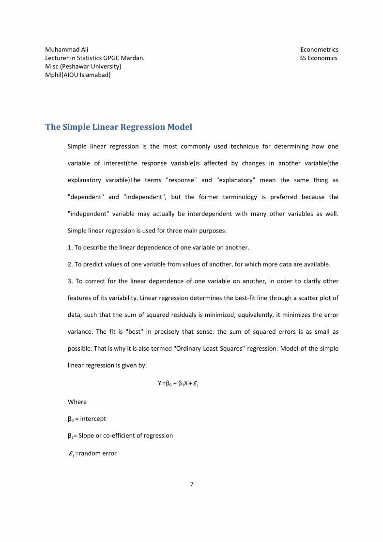
The Simple Linear Regression Model

Simple linear regression is the most commonly used technique for determining how one

variable of interest(the response variable)is affected by changes in another variable(the

explanatory variable)The terms "response" and "explanatory" mean the same thing as

"dependent" and "independent", but the former terminology is preferred because the

"independent" variable may actually be interdependent with many other variables as well.

Simple linear regression is used for three main purposes:

1. To describe the linear dependence of one variable on another.

2. To predict values of one variable from values of another, for which more data are available.

3. To correct for the linear dependence of one variable on another, in order to clarify other

features of its variability. Linear regression determines the best-fit line through a scatter plot of

data, such that the sum of squared residuals is minimized; equivalently, it minimizes the error

variance. The fit is "best" in precisely that sense: the sum of squared errors is as small as

possible. That is why it is also termed "Ordinary Least Squares" regression. Model of the simple

linear regression is given by:

Yi=β0 + β1Xi+ iε

Where

β0 = Intercept

β1= Slope or co-efficient of regression

iε =random error





8

An important objective of regression analysis is to estimate the unknown parameters β0 and β1 in the

regression model. This process is also called fitting the model to the data, The parameters β0 and β1 are

usually called regression coefficients. The slope β1 is the change in the mean of the distribution of Y

producing a unit change in X. The intercept β0 is the mean of the distribution of the response variable Y

when X=0.

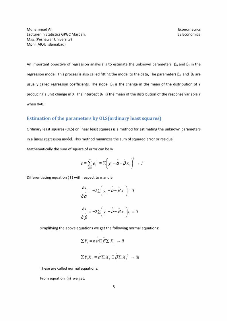
Estimation of the parameters by OLS(ordinary least squares)

Ordinary least squares (OLS) or linear least squares is a method for estimating the unknown parameters

in a linear regression model. This method minimizes the sum of squared error or residual.

Mathematically the sum of square of error can be w

∑=

→

−−∑==n

iiii Ixyes

1

2^^2 βα

Differentiating equation ( I ) with respect to α and β

02

02

^^

^

^^

^

=

−−∑−=∂

∂

=

−−∑−=∂

∂

iii

ii

xxys

xys

βαβ

βαα

simplifying the above equations we get the following normal equations:

iiiXXXY

iiXnY

iiii

ii

→∑+∑=∑

→∑+=∑

2^^

^^

βα

βα

These are called normal equations.

From equation (ii) we get:

Muhammad Ali

Lecturer in Statistics GPGC Mardan.



Now substituting the value of α

Y

Y

Y

^

^

=

=

∑

∑

∑

β

β

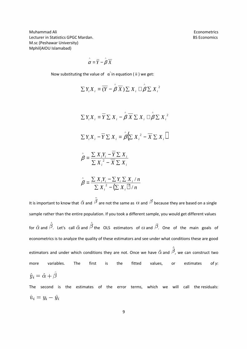
It is important to know that and

sample rather than the entire population. If you took

for and . Let's call and

econometrics is to analyze the quality of these estimators and see under what conditions these are good

estimators and under which conditions they are not.

more variables. The

The second is the estimates of the error terms, which we will call the


9

XY^^

βα −=

Now substituting the value of αᶺ in equation ( ii ) we get:

( )

( ) nXX

nXYYX

XXX

XYYX

XXXXYXY

XXXXYXY

XXXYXY

ii

iiii

ii

iii

iiiii

iiiii

iiii

/

/

)(

22

2

2^

2^^

2^^

∑−∑

∑∑−∑=

∑−∑

∑−∑=

∑−∑=∑−

∑+∑−∑=

∑+∑−=

β

ββ

ββ

and are not the same as and because they are based on a single

sample rather than the entire population. If you took a different sample, you would get different values

and the OLS estimators of and . One of the main goals of


d under which conditions they are not. Once we have and

ore variables. The first is the fitted values, or estimates of

The second is the estimates of the error terms, which we will call the

Econometrics

BS Economics

because they are based on a single

a different sample, you would get different values

. One of the main goals of


, we can construct two

fitted values, or estimates of y:

The second is the estimates of the error terms, which we will call the residuals:





10

Assumptions of the Classical linear Regression Model:

Following are the few important assumptions of the classical linear regression model:

1. Linearity: The regression model is linear in the parameters. i.e.

Yi =β0 +β1Xi + ui

2. Non stochastic X: Values of the independent or repressor variable assumed to be fixed in

the repeated sampling.

3. Zero mean of the error term: The expected value or mean of the random disturbance

term given the value of X is zero. i.e.

E ( Ui/Xi) = 0

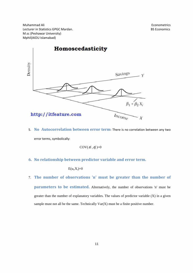
4. Homoscedasticity: Variance of the ui for all the observations remain the same.i.e.

V ( u1) = δ2 V(u2) = δ

2 V(u3) = δ

2 … V(un)=δ

2

Muhammad Ali




5. No Autocorrelation between error term

error terms, symbolically:

6. No relationship between predictor va

7. The number of observations 'n' must be greater than the number of

parameters to be

greater than the number of explanatory

sample must not all be the same. Technically Var(X) must be a finite positive number.


11

correlation between error term: There is no correlation between any two

symbolically:

COV( iε , jε )=0

No relationship between predictor variable and error term.

E(ui,Xi)=0

The number of observations 'n' must be greater than the number of

parameters to be estimated. Alternatively, the number of observations 'n' must be

greater than the number of explanatory variables. The values of predictor variable (X) in a given


Econometrics

BS Economics

There is no correlation between any two

riable and error term.

The number of observations 'n' must be greater than the number of

, the number of observations 'n' must be

tor variable (X) in a given


Muhammad Ali




8. The regression model is correctly specified.

bias or error in the model used in empirical

, there are no perfect linear relationships among the explanatory variables.

Interpretation of Coeffiffiffiffi

The interpretation of the coeffi

estimated intercept (b0) tells us the value of y that is expected when x = 0. This is

because many of our variables don’t have true 0 values (or at least not

income, which rarely if ever have 0 values). The slope (b1) is

relationship between x and y. It is interpreted as the

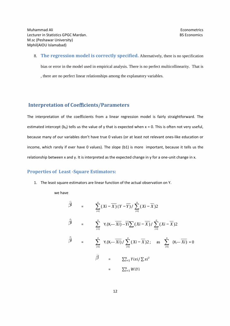
Properties of Least -Square Estimators:

1. The least square estimators are lin

we have


12

The regression model is correctly specified. Alternatively, there is no specification

bias or error in the model used in empirical analysis. There is no perfect multicollinearity. That is


ffiffiffifficients/Parameters

fficients from a linear regression model is fairly straig

) tells us the value of y that is expected when x = 0. This is

because many of our variables don’t have true 0 values (or at least not relevant ones

have 0 values). The slope (b1) is more important, because it tells us the

relationship between x and y. It is interpreted as the expected change in y for a one

Square Estimators:

The least square estimators are linear function of the actual observation on Y.

= ∑=

−n

i

XXi1

)( ( )YY − / ∑=

−n

i

XXi1

2)(

= ∑=

n

i 1

Yi (Xi--- )Xi -- ∑ − )( XXiYi / ∑=

n

i

Xi1

(

= ∑=

n

i 1

Yi (Xi--- )Xi / ∑=

−n

i

XXi1

2)( ; as

= ∑ ��/∑��

2

= ∑ ��

�

Econometrics

BS Economics

Alternatively, there is no specification

is no perfect multicollinearity. That is


cients from a linear regression model is fairly straightforward. The

) tells us the value of y that is expected when x = 0. This is often not very useful,

relevant ones-like education or

important, because it tells us the

expected change in y for a one-unit change in x.

ear function of the actual observation on Y.

− XXi 2)

∑=

n

i 1

(Xi--- )Xi = 0

Muhammad Ali




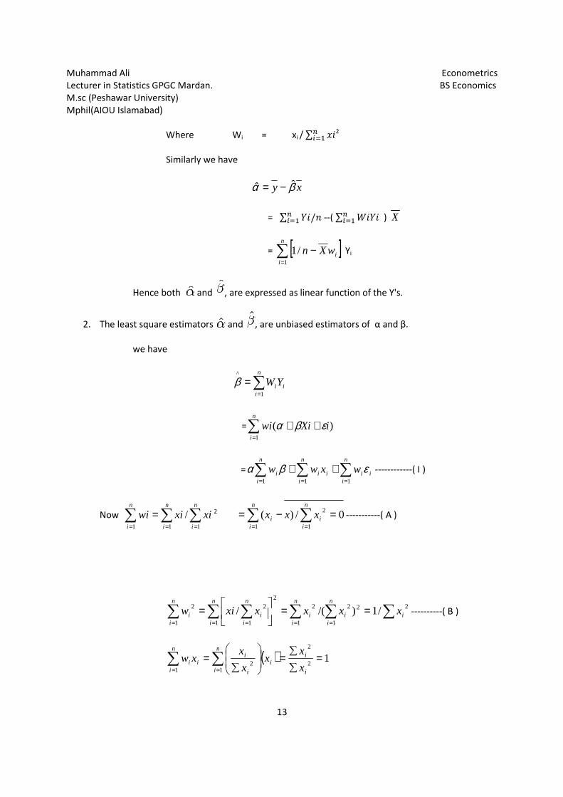
Where

Similarly we have

Hence both and

2. The least square estimators

we have

Now ∑ ∑ ∑= = =

=n

i

n

i

n

i

xiwi1 1 1

/

∑=

n

iiw

1

2

∑

=

n

iii xw

1


13

Wi = xi / ∑ ��

2

Similarly we have

xy βα ˆˆ −=

= ∑ ��/�� --( ∑ ��

� ) X

= [ ]∑=

−n

iiwXn

1

/1 Yi

and , are expressed as linear function of the Y's.

The least square estimators and , are unbiased estimators of α and β.

∑=

=n

iiiYW

1

^

β

=∑=

++n

i

iXiwi1

)( εβα

= ∑ ∑ ∑

= = =

++n

i

n

i

n

iiiiii wxww

1 1 1

εβα ------------

∑ xi1

2 ∑ ∑

= =

=−=n

i

n

iii xxx

1 1

2 0/)( -----------( A )

∑ ∑ ∑ ∑∑= = ==

==

=n

i

n

i

n

iii

n

ii xxxxxi

1 1 1

2222

1

2 /1)/(/

( )∑=

=∑

∑=

∑=

n

i i

ii

i

ii

x

xx

x

x

12

2

21

Econometrics

BS Economics

X

, are expressed as linear function of the Y's.

, are unbiased estimators of α and β.

------------( I )

( A )

ix 2----------( B )

Muhammad Ali




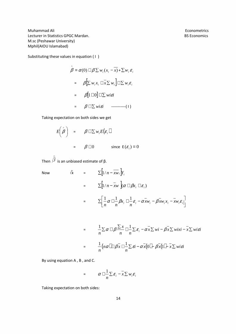
Substituting these values in equation ( I )

^

β (= α

= β

=

=

Taking expectation on both sides we g

^

βE =

=

Then is an unbiased estimate of β.

Now

By using equation A , B , and C.

Taking expectation on both sides:


14

n equation ( I )

)()0( xxw ii −∑+ β + iiw ε∑

[ ] iiiii wwxxw εβ ∑+∑+∑

[ ] iwiεβ ∑++ 01

iwiεβ ∑+ -----------( I )

Taking expectation on both sides we get

( )ii Ew εβ ∑+

0+β since E 0)( =iε

is an unbiased estimate of β.

= [ ] ii Yxwn −∑ /1

= [ ] )(/1 iixwxn εβα ++−∑

=

−−++∑ iiii xwxwxn

xnn

βαεβα 111

= wixnn

x

n i βαεβα −∑−∑+∑+∑11

= ( ) ( ) ( )xxin

xnn

βαεβα −−−∑++ 1011

By using equation A , B , and C.

= iii wxn

εεα ∑−∑+ 1

Taking expectation on both sides:

Econometrics

BS Economics

− iii wxx ε

iwixwixix εβ ∑−∑

iwix ε∑−

Muhammad Ali




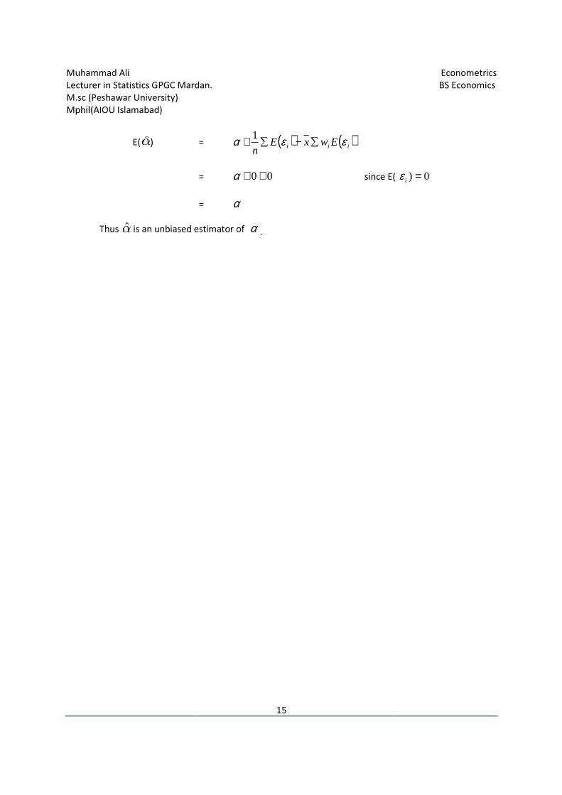
E( )

Thus is an unbiased estimator of


15

= ( ) ( )iii EwxEn

εεα ∑−∑+ 1

= 00++α since E(

= α

is an unbiased estimator of α .

Econometrics

BS Economics

since E( 0) =iε





16

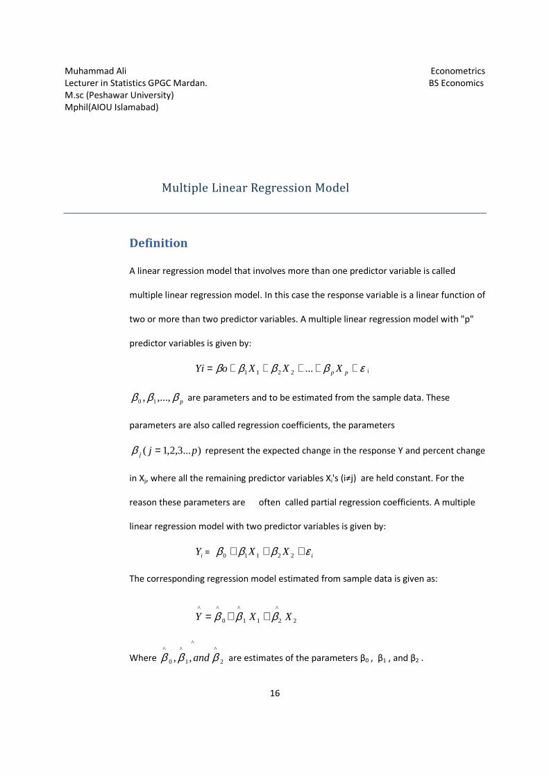
Multiple Linear Regression Model

Definition

A linear regression model that involves more than one predictor variable is called

multiple linear regression model. In this case the response variable is a linear function of

two or more than two predictor variables. A multiple linear regression model with "p"

predictor variables is given by:

εββββ +++++= pp XXXoYi ...2211 i

pβββ ,...,, 10 are parameters and to be estimated from the sample data. These

parameters are also called regression coefficients, the parameters

)...3,2,1( pjj =β represent the expected change in the response Y and percent change

in Xj, where all the remaining predictor variables Xi's (i≠j) are held constant. For the

reason these parameters are often called partial regression coefficients. A multiple

linear regression model with two predictor variables is given by:

iY = iXX εβββ +++ 22110

The corresponding regression model estimated from sample data is given as:

2

^

211

^

0

^^

XXY βββ ++=

Where

^

2

^

1

^

0

^

,, βββ and are estimates of the parameters β0 , β1 , and β2 .





17

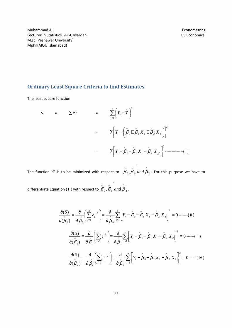
Ordinary Least Square Criteria to find Estimates

The least square function

S = e∑ i2

= ∑=

−n

ii YY

1

2^

=

2

22

^

11

^

0

^

++−∑ XXYi βββ

=

2

22

^

11

^

0

^

2

−−−∑ XXYi βββ --------------( I )

The function 'S' is to be minimized with respect to

^

2

^

1

^

0

^

,, βββ and . For this purpose we have to

differentiate Equation ( I ) with respect to

^

2

^

1

^

0

^

,, βββ and .

∑∑==

=

−−−∂

∂=

∂

∂=∂

∂ n

ii

n

ii

XXYeS

1

2

22

^

11

^

0

^

0

^1

2

^

00

^0

)(

)( ββββββ

-------( II )

∑∑==

=

−−−∂

∂=

∂

∂=∂

∂ n

ii

n

ii XXYe

S

1

2

22

^

11

^

0

^

1

^1

2

^

11

^0

)(

)( ββββββ

------( III)

∑∑==

=

−−−∂

∂=

∂

∂=∂

∂ n

ii

n

ii

XXYeS

1

2

22

^

11

^

0

^

2

^1

2

^

22

^0

)(

)( ββββββ

----( IV )





18

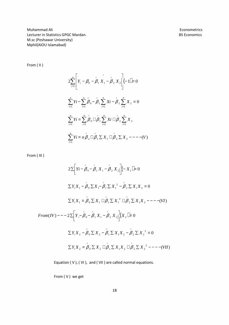
From ( II )

( ) 0121

^

22

^

11

^

0 =−

−−−∑

=

n

ii XXY βββ

∑ ∑∑∑= ===

=−−−n

i

n

i

n

i

n

i

XXiYi1 1

22

^

11

^

0

^

1

0βββ

∑ ∑∑∑= ===

++=n

i

n

i

n

i

n

i

XXiYi1 1

22

^

11

^

0

^

1

βββ

)(22

^

11

^^

1

VXXnYi o

n

i

−−−−∑+∑+=∑=

βββ

From ( III )

( ) 02 122

^

11

^

0

^

=−

−−−∑ XXXYi βββ

0212

^2

11

^

10

^

1 =∑−∑−∑−∑ XXXXXYi βββ

)(212

^2

11

^

10

^

1 VIXXXXXYi −−−−∑+∑+∑=∑ βββ

( ) 02)( 222

^

11

^

0

^

=

−−−∑−−− XXXYIVFrom i βββ

0222

^

211

^

20

^

2 =∑−∑−∑−∑ XXXXXYi βββ

)(222

^

211

^

20

^

2 VIIXXXXXYi −−−−∑+∑+∑=∑ βββ

Equation ( V ), ( VI ), and ( VII ) are called normal equations.

From ( V ) we get





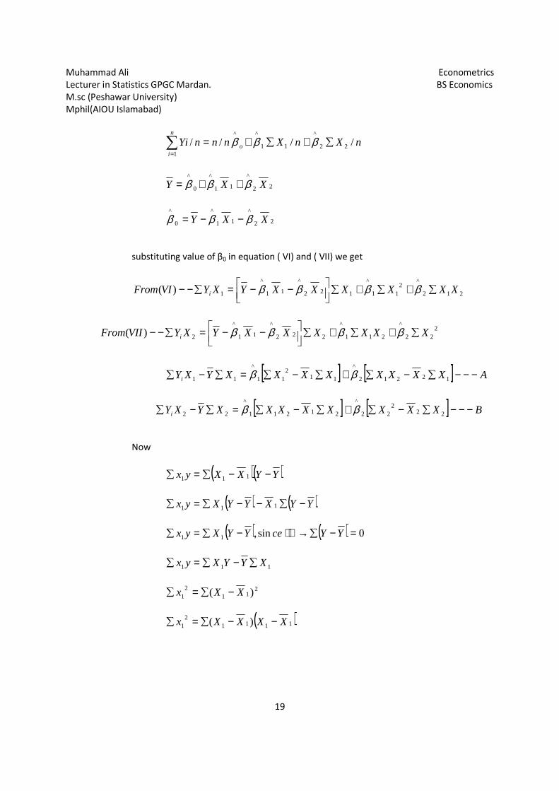
19

nXnXnnnYi o

n

i

//// 22

^

11

^^

1

∑+∑+=∑=

βββ

22

^

11

^

0

^

XXY βββ ++=

22

^

11

^

0

^

XXY βββ −−=

substituting value of β0 in equation ( VI) and ( VII) we get

212

^2

11

^

122

^

11

^

1)( XXXXXXYXYVIFrom i ∑+∑+∑

−−=∑−− ββββ

222

^

211

^

222

^

11

^

2)( XXXXXXYXYVIIFrom i ∑+∑+∑

−−=∑−− ββββ

[ ] [ ] AXXXXXXXXYXYi −−−∑−∑+∑−∑=∑−∑ 12212

^

112

11

^

11 ββ

[ ] [ ] BXXXXXXXXYXYi −−−∑−∑+∑−∑=∑−∑ 222

22

^

21211

^

22 ββ

Now

( )( )YYXXyx −−∑=∑ 111

( ) ( )YYXYYXyx −∑−−∑=∑ 111

( ) ( ) 0sin,11 =−∑→−∑=∑ YYceYYXyx

111 XYYXyx ∑−∑=∑

211

21 )( XXx −∑=∑

( )11112

1 )( XXXXx −−∑=∑





20

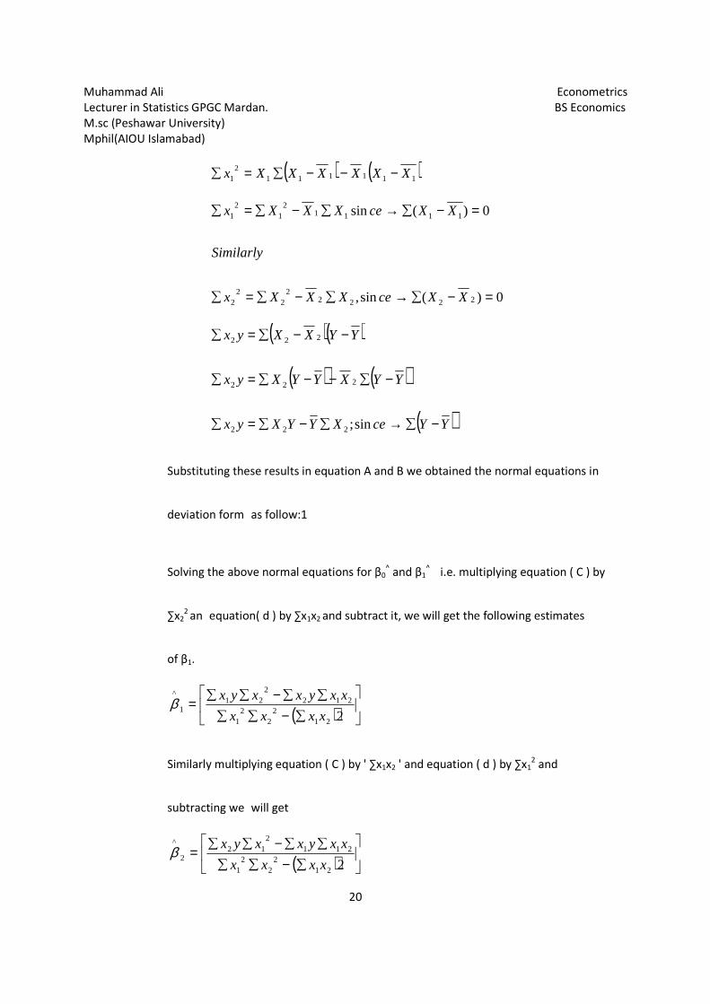
( ) ( )1111112

1 XXXXXXx −−−∑=∑

0)(sin,

0)(sin

22222

22

2

11112

12

1

=−∑→∑−∑=∑

=−∑→∑−∑=∑

XXceXXXx

Similarly

XXceXXXx

( )( )

( ) ( )

( )YYceXYYXyx

YYXYYXyx

YYXXyx

−∑→∑−∑=∑

−∑−−∑=∑

−−∑=∑

sin;222

222

222

Substituting these results in equation A and B we obtained the normal equations in

deviation form as follow:1

Solving the above normal equations for β0^ and β1

^i.e. multiplying equation ( C ) by

∑x22

an equation( d ) by ∑x1x2 and subtract it, we will get the following estimates

of β1.

( )

∑−∑∑

∑∑−∑∑=

2212

22

1

2122

211

^

xxxx

xxyxxyxβ

Similarly multiplying equation ( C ) by ' ∑x1x2 ' and equation ( d ) by ∑x12 and

subtracting we will get

( )

∑−∑∑

∑∑−∑∑=

2212

22

1

2112

122

^

xxxx

xxyxxyxβ





21

Standardized coefficients:

In statistics, standardized coefficients or beta coefficients are the estimates resulting from an analysis

carried out on independent variables that have been standardized so that their variances are. Therefore,

standardized coefficients refer to how many standard deviations a dependent variable will change,

per standard deviation increase in the predictor variable. Standardization of the coefficient is usually

done to answer the question of which of the independent variables have a greater effect on

the dependent variable in a multiple regression analysis, when the variables are

measuredindifferent unitsof (forexample, income measuredin dollars and familysize measuredin numbe

r of individuals). A regression carried out on original (unstandardized) variables produces unstandardized

coefficients. A regression carried out on standardized variables produces standardized coefficients.

Values for standardized and unstandardized coefficients can also be derived subsequent to either type

of analysis. Before solving a multiple regression problem, all variables (independent and dependent) can

be standardized. Each variable can be standardized by subtracting its mean from each of its values and

then dividing these new values by the standard deviation of the variable. Standardizing all variables in a

multiple regression yields standardized regression coefficients that show the change in the dependent

variable measured in standard deviations.

Advantages

Standard coefficients' advocates note that the coefficients ignore the independent variable's scale of units,

which makes comparisons easy.





22

Disadvantages

Critics voice concerns that such a standardization can be misleading; a change of one standard deviation

in one variable has no reason to be equivalent to a similar change in another predictor. Some

variables are easy to affect externally, e.g., the amount of time spent on an action. Weight or

cholesterol level are more difficult, and some, like height or age, are impossible to affect externally.

Goodness of Fit (R2)

The Coefficient of Determination, also known as R Squared, is interpreted as the goodness of fit of a

regression. The higher the coefficient of determination, the better the variance that the dependent

variable is explained by the independent variable. The coefficient of determination is the overall

measure of the usefulness of a regression. For example, if R2 is 0.95. This means that the variation in the

regression is 95% explained by the independent variable. That is a good regression. Now, if the

Coefficient of Determination, or R2,is 0.50. Its means that the variation in the regression is 50%

explained by the independent variable. This is not a good regression. Note that R2

lies between '0' and

'1'. If R2=1, it means that the fitted model explains 100% of the variation in response variable 'Y'. On the

other hand if R2=0, the model does not explain any of the variation of 'Y'. The Coefficient of

Determination can be calculated as the Regression sum of squares, RSS, divided by the total sum of

squares,SST

Coefficient of Determination = TSS

RSS

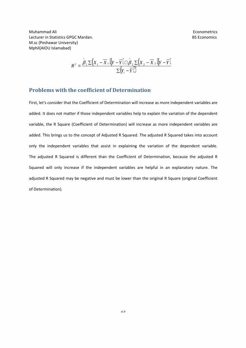
Mathematical formula of the coefficient of Determination is given as under:





23

Problems with the coefficient of Determination

First, let's consider that the Coefficient of Determination will increase as more independent variables are

added. It does not matter if those independent variables help to explain the variation of the dependent

variable, the R Square (Coefficient of Determination) will increase as more independent variables are

added. This brings us to the concept of Adjusted R Squared. The adjusted R Squared takes into account

only the independent variables that assist in explaining the variation of the dependent variable.

The adjusted R Squared is different than the Coefficient of Determination, because the adjusted R

Squared will only increase if the independent variables are helpful in an explanatory nature. The

adjusted R Squared may be negative and must be lower than the original R Square (original Coefficient

of Determination).

( )( ) ( )( )( )2

222

^

111

^

2

YY

YYXXYYXXR

i −∑

−−∑+−−∑= ββ

econometrics notes (introduction, simple linear regression, multiple linear regression)

Education