lis working paper series · we thank koen caminada, ... 2012 nig conference in leuven, and the 2013...

LIS Working Paper Series

Luxembourg Income Study (LIS), asbl

No. 595

Sectoral trends in earnings inequality and employment

International trade, skill-biased technological change, or labour market institutions?

Stefan Thewissen, Chen Wang, and Olaf van Vliet

July 2013

Sectoral trends in earnings inequality and employment

International trade, skill-biased technological change, or labour market institutions?1

Submission to LIS Working Paper Series

Stefan Thewissen, Chen Wang, and Olaf van Vliet

Department of Economics, Leiden University

P.O. Box 9520, 2300 RA Leiden, the Netherlands

Phone: ++31 71 527 7756

[email protected]

[email protected]

[email protected]

Abstract

Current studies addressing the rise in inequality confine themselves to country-level

developments. This paper delineates trends in earnings inequality and employment at the

sectoral level for eight LIS countries between 1985-2005. Earnings inequality mainly

manifests itself within rather than between sectors. Yet, there is significant variation in the

level of inequality across sectors whilst the differences between countries in intrasectoral

inequality are much less pronounced. A general rise in intrasectoral earnings dispersion and a

shift from the manufacturing industry towards the financial sector are perceptible. Cross-

sectional pooled time-series analyses indicate significant associations between the exposure to

import and decreased employment within sectors, whilst no evidence is found for relations

between earnings inequality and international trade or skill-biased technological change.

Keywords

Earnings inequality, sectoral approach, globalisation, skill-biased technological change,

income inequality

JEL codes

D30; D63; E24; L60

1 This study is part of the research programme ‘Reforming Social Security’ of Leiden University. Chen Wang is

funded by the Chinese Scholarship Council. We thank Koen Caminada, Kees Goudswaard, the participants at the

2012 Dutch Economists day in Amsterdam, the UM/ICIS Measuring Globalisation workshop in Maastricht, the

2012 NIG conference in Leuven, and the 2013 ILERA Amsterdam conference for their helpful comments. The

usual disclaimer applies.

mailto:[email protected]



2

1. Introduction

A widely observed phenomenon in social sciences is the gradual and widespread increase in

income inequality in developed countries (e.g., Brandolini and Smeeding, 2008; 2009; OECD,

2008; 2011a; Autor et al., 2013). In general this trend is attributed to widening labour

earnings (Kenworthy and Pontusson, 2005; Immervoll and Richardson, 2011; Caminada et

al., 2012).

Even though much attention has been given to these inequality trends at the country

level, much less has been written on developments within countries across different sectors.

Questions that remain unanswered are to what extent these higher levels of inequality are a

consequence of larger differences in average earnings between industries, or a higher earnings

dispersion within industries. Another possible explanation is that there has been loss of

employment within certain sectors. Furthermore, it is unclear if these tendencies in earnings

and employment took place in all sectors and in all countries, or whether differences between

sectors can be observed. Lastly, in case there is heterogeneity across sectors or countries, we

do not know what can account for these differences.

This study describes trends in labour earnings inequality and employment at the

sectoral level in eight LIS countries between 1985 and 2005 based on a new database (Wang

et al., 2013). By means of a decomposition we depict that the bulk of earnings inequality at

the country level is a consequence of inequality within rather than between sectors. The level

of intrasectoral inequality differs significantly across sectors, with agriculture, finance, and

wholesale as relatively unequally distributed sectors, and mining and utilities as the most

equally distributed sectors. Our calculations denote a rise in sectoral earnings inequality that

is widespread across sectors, corresponding to the rise of inequality at the country level.

During the period under scrutiny a notable shift from the manufacturing industry towards the

financial sectors took place. These sectoral trends do not differ much across countries.

Using cross-sectional pooled time-series analyses we test three possible determinants

of these sectoral trends that are often put forward to explain the upsurge in inequality at the

country level, namely, international trade, skill-biased technological change, and changes in

labour market institutions. As for the first two sets of factors sectoral data are available, we

inspect whether sectors more exposed to trade or technological change embody higher

earnings inequality or job loss. In this way we allow for heterogeneity across sectors due to

imperfect labour mobility, which contributes to the existing knowledge on the effects of

international trade and technological change based on country-level information. We do not

find positive associations between international trade or technological change and earnings

3

inequality. Nonetheless, there is robust evidence for a decrease in relative employment in

import-competing industries. Lastly, we find a relation between decreased trade union

influence at the country level and sectoral earnings inequality.

Empirically, our approach is in between the inequality literature, which generally

bases its conclusions on the distribution of household earnings (Mahler et al., 1999;

Brandolini and Smeeding, 2008; 2009; Checchi and García-Peñalosa, 2008), and the

(Mincerian) wage literature which by and large employs individual earnings and generally

analyses skill demand or polarisation rather than inequality per se (Acemoglu, 2003a; 2003b;

Autor et al., 2003; Michaels et al., forthcoming). From the inequality literature we take the

dependent variable, as our main objective is to analyse how increased earnings inequality at

the country level is manifested at the sectoral level. Yet, we base our main findings on

individual earnings, which is common in the wage literature, rather than summing and

equivalising the earnings at the household level. In this way we can attribute earnings to

sectors with less noise, as we do not attribute all household earnings to the sector in which the

household head is working regardless if the spouse or other relatives are working in that

sector as well.

In the inequality literature our sectoral design is relatively new. The approach allows

for heterogeneity between sectors due to imperfect labour mobility. Compared to the existing

studies (Mahler et al., 1999; OECD, 2011a; Michaels et al., forthcoming) who only calculate

sectoral information at two moments in time, we seek to contribute to the literature by

building a new database on inequality and employment at the sectoral level that contains

sectoral data over a longer period. This allows us to conduct cross-section panel regressions,

in which we can control for certain unobserved and observed industry-specific and country-

specific developments. Second, as opposed to the sectoral studies from the wage literature

(OECD, 2011a; Michaels et al., forthcoming), we do not only explore earnings but also

sectoral employment indicators separately. Compared to Mahler et al. (1999), who also use

LIS data, we base our findings on individual rather than household earnings, so that we can

attribute information to sectors with less noise.

The remainder of the paper is structured as follows. Section 2 gives a description of

the dataset and the used indicators. Next, in Section 3, the trends at the country and sectoral

level are presented. In Section 4 we expound on three possible explanations for our sectoral

trends, which are subsequently analysed in Section 5. Section 6 concludes.

4

2. Data section

2.1 Income definition, sector standardisation, and sample

To calculate the level of labour earnings inequality at the sectoral level this paper makes use

of the Leiden LIS Sectoral Income Inequality Dataset (Wang et al., 2013).2 This database is

constructed on the basis of the Luxembourg Income Study (LIS) micro data. Appendix 2

provides background information and descriptives for the database, and Appendix 3 gives a

full overview of the variables that are included in the dataset.

Elaborating on the approach laid down by Mahler et al. (1999) we confine our sample

to individuals aged between 25 and 54, which are those people most dependent on earnings as

source of income. Since we are interested in labour earnings inequality, we only include

income from wages and salaries or self-employment, omitting income from other sources,

such as interest and rent, and we do not adjust the wages for taxes or social contributions. We

refer to this income definition as earnings for the remainder of this paper. For all calculations

we comply with standard LIS top- and bottom coding conventions, with 1 per cent of mean

earnings as the bottom, and ten times the median earnings as the top boundary. Even though

this procedure reduces the influence of outliers, a disadvantage of this approach is that

enrichment at the top is left out of the analysis (Atkinson et al., 2011).

We explicitly dissent from the inequality literature convention as for instance Mahler

et al. (1999) do, to sum and equivalise earnings at the household level. The main problem

with summing earnings at the household level is that in that way earnings or employment

information from the spouse or other relatives are attributed to the sector in which the

household head is working, even though the other household members work in a different

sector than the household head. As a sensitivity test, we also show results for household-level

earnings and for individual earnings in which we restrict our sample to household heads only.

We standardise the sectoral information by means of the International Standard of

Industrial Classification (ISIC) rev. 3.0 at the two and three digit level.3 Table 1 provides the

full set of included sectors. The two-digit level distinguishes between the main nine

industries. We use the three-digit level to further break down the manufacturing and transport

2 This dataset is available at www.hsz.leidenuniv.nl.

3 Sometimes this required some interpretation or the exclusion of some sectors (mainly manufacturing of

transport equipment and recycling); the classification scheme is available as a worksheet in Wang et al. (2013).

Evidence that the classification scheme is reliable comes from the correlation between the relative employment

size of the sectors based on our data and data available from OECD STAN. This correlation is for all countries

around 0.93.

http://www.hsz.leidenuniv.nl/

5

and telecommunication sector into 12 subsectors, as in Mahler et al. (1999), OECD (2011a),

and Michaels et al. (forthcoming).4

Table 1 Industry classification Two-digit ISIC sectors Three-digit ISIC subsectors

1. Agriculture and fishing (none)

2. Mining and quarrying (none)

3. Manufacturing 31. Manufacturing of food products, beverages, and tobacco

32. Manufacturing of textiles, textile products, leather, and

footwear

33. Manufacturing of wood and products of wood and cork

34. Manufacturing of pulp, paper, paper products, printing, and

publishing

35. Manufacturing of chemical, rubber, plastics, and fuel products

36. Manufacturing of other non-metallic mineral products

37. Manufacturing of basic metals and fabricated metal products

38. Manufacturing of machinery and equipment)

39. Manufacturing of transport equipment

30. Other manufacturing (n.e.c. and recycling)

4. Electricity, gas, and water (none)

5. Construction (none)

6. Wholesale and retail trade, restaurants and

hotels

(none)

7. Transport and telecommunications 71. Transport

72. Telecommunications

8. Finance, insurance, real estate, and business (none)

9. Community, social, and personal services (none)

Sectoral information is available for eight OECD countries as listed in Table 2, allowing us to

compose an unbalanced panel of five periods of five years each in between around 1985 up to

and including around 2005.5 In total we have 31 waves and 651 observations at the sectoral

level.

Table 2 Country sample Country Waves

1. Czech Republic 1996, 2004

2. Denmark 1987, 1992, 1995, 2000, 2004

3. Finland 1987, 1991, 1995, 2000, 2004

4. Germany 1984, 1989, 1994, 2000, 2004

5. Ireland 1994-1996, 2004

6. Sweden 1987, 1992, 2000, 2005

7. UK 1986, 1999, 2004

8. US 1986, 1991, 1994, 2000, 2004

Note: We combine the 1994-1996 waves for Ireland where we recalculate the earnings information to 1995 levels using

information on inflation from the World Bank (2012).

4 Unfortunately, no further breakdown in the community services sector is possible with LIS micro data for a

sufficient number of country-period observations. The community sector consists of people working in public

administration, education, health and social work, and other community and personal service activities. 5 For Spain in 1995 and 2000 information at the sectoral level is available as well, but the number of surveyed

people is too low to calculate levels of inequality at a disaggregated level with sufficient confidence. Belgium is

excluded as only data on net earnings are available. For Poland data are available, but not for our indicator for

skill-biased technological change, thus we exclude it altogether.

6

2.2 Earnings inequality at the country level

We make use of two indicators to calculate the earnings inequality. The mean log deviation

(MLD) or GE(0) is more sensitive to fluctuations at the bottom end of the distribution,

whereas the Gini coefficient is more sensitive to changes across the mean of the distribution

(Atkinson, 1970). We start by calculating the earnings inequality based on our earnings

definition at the country level for both indicators. We subsequently decompose the MLD into

a part within and a part between sectors, as this indicator has the advantage of not leaving a

residual. This decomposition is defined as follows6, with sectors indexed { }

weighted by their share of employed individuals , where the sector includes the individuals

indexed { } with earnings , weight , and arithmetic mean earnings :

∑

∑

∑

(

) ∑ (

)

(1)

The first element on the right-hand side of equation (1) denotes inequality within industries,

calculated as the sum of the MLD in all separate sectors weighted by the (weighted) number

of individuals working in the sector relative to the total (weighted) number of working

individuals. The second part summarises the between-sector part, which are the arithmetic

mean earnings in sector as a fraction of the mean earnings of the total population.

2.3 Earnings inequality at the sectoral level

Next, we analyse earnings inequality trends at the sectoral level. To this end we apply the

MLD and the Gini index. The MLD at the sectoral level is defined in the following fashion:

∑

∑

( )

(2)

The Gini coefficient has the advantages of being the most frequently used inequality measure

in the literature, and it can be corrected for underestimation bias in case of small sample sizes.

Therefore, we use this indicator for the descriptive trends.7 Using Monte Carlo simulations for

6 See Kampelmann (2009) for a general discussion on inequality measures, including an appendix with a

decomposition of the MLD that can be transposed to ours. 7 The correlation between the first-order corrected Gini index and the MLD at the sectoral level is 0.88.

7

different cumulative distributions, Deltas (2003) shows that the Gini index can understate the

‘true’ inequality level when the sample size is relatively low (roughly from ). By

multiplying the Gini index by

, which Deltas calls the first order correction, the

underestimation bias is significantly reduced.8 The first order corrected Gini index at the

sectoral level then becomes:

{∑

∑

∑

∑

( )}

(3)

2.4 Employment measures at the sectoral level

Increased income inequality at country level might be not so much a consequence of widening

earnings distribution, but rather of employment loss (Gottschalk and Smeeding, 1997;

Atkinson, 2003; Kenworthy and Pontusson, 2005). Even though the LIS database allows for

the standardised calculation of sectoral earnings inequality for multiple countries over time

(Förster and Vleminckx, 2004; Mahler and Jesuit, 2006), unfortunately, it is not possible to

track individual employment shifts over time. This is due to the fact that the LIS database is a

time series rather than a panel at the individual level.

Using a number of proxies we try to depict employment effects at the sectoral level in

an indirect fashion. First, we use own data based on LIS (Wang et al., 2013) and OECD

STAN data (2011b) on the relative employment size of sectors to map total labour shifts

between sectors. The relative employment size is defined as the number of persons engaged

per industry divided by the total number of persons engaged in a country.9 We show our own

data for the descriptives.10

Second, following Mahler et al. (1999), we also calculate the

relative median wage, defined as the sectoral median labour earnings divided by the national

median labour earnings. The relative median earnings in a sector will increase when job loss

mainly occurs at the lower end of the earnings distribution.11

8 As an alternative to the first order correction to correct for small samples, we also conduct the regressions

leaving out the sectors with , which does not affect the results. 9 This indicator is only sensitive to net changes at the extensive rather than intensive margin, as it measures the

number of persons engaged rather than the number of working hours. 10

The correlation between the relative employment size from our data and the OECD STAN data is 0.93. 11

Both employment indicators that we constructed are amended for the person weight as provided by LIS.

8

3. Trends in inequality over time, across countries, and across industries

3.1 Trends at the country level

Figure 1 shows the trends in inequality at the country level when all sectors are pooled, using

our Leiden LIS Sectoral Income Inequality dataset. The calculations are based on the same

sample as used in the regressions, thus, all individuals aged 25-54 with non-zero earnings

excluding those not classified in a sector.

Figure 1 Earnings inequality at the country level 1985-2005

1a Gini index

1b Mean log deviation

Source: Leiden LIS Sectoral Income Inequality Dataset

As can be deduced from Figure 1 inequality is the highest in the Anglo-Saxon countries, and

considerably lower in the Northern countries. As is widely documented in the literature,

0.25

0.30

0.35

0.40

0.45

1985 1990 1995 2000 2005

Czech republic

Denmark

Finland

Germany

Ireland

Sweden

United Kingdom

United States

Mean

0.15

0.20

0.25

0.30

0.35

1985 1990 1995 2000 2005

Czech republic

Denmark

Finland

Germany

Ireland

Sweden

United Kingdom

United States

Mean

9

earnings are growing wider apart within countries over time (OECD, 2008; 2011a; Brandolini

and Smeeding, 2008; 2009; Immervoll and Richardson, 2011; Caminada et al., 2012). The

strongest increase took place between 1995 and 2000. In addition, we see a strong upsurge in

especially the MLD of Germany; up to around 1990 the earnings inequality was still below

average, rising up to a level just below the United Kingdom around 2005. This is likely to be

at least partly a consequence of the unification as the LIS waves of 1984 and 1989 are based

on West Germany only12

(see also Fuchs-Schündeln et al., 2010).

Even though the MLD is characterised by a more erratic course, its trend is by and

large comparable to the one shown for the Gini coefficient. A noticeable exception is Finland,

where the Gini index shows a gradual descent whilst the MLD drops rather abruptly from

1995 to 2000. It implies that during this period the earnings inequality at the bottom end of

the distribution decreased more rapidly than around the middle. Further inspection shows that

inequality at the top half of the distribution actually increased as measured by the GE(2), as

also found by Cowell and Fiorio (2011), even though they base their analysis on disposable

household income from LIS data. This provides an explanation why the Gini index decreases

less rapidly than the MLD.

Next, we decompose the MLD into a part within and a part between sectors, as shown

in Table 3. Columns 1-3 show the level of earnings inequality at the country level and the

fourth one denotes the increase over time. Columns 5-7 summarise the percentage of the

MLD at the country level due to inequality within industries.

Table 3 shows that the lion’s share of inequality is a result of earnings dispersion

within industries, rather than differences in average earnings between industries.13

On

average, within-industry inequality accounted for a larger share of the inequality at the

country level over time.

From the decomposition it cannot be inferred that sectoral variation is not important in

understanding country-level inequality – it only shows that the variation within sectors is

more pronounced than the average wage differences between sectors. In particular, as we

show in the next section, there is substantial variation in the levels of inequality across sectors

– in fact, this variation is more pronounced than the country-level differences.

12

The waves 1984 and 1989 for Germany are not included in the regressions as no sectoral information on

import or export is available. 13

Of course, the share of inequality between groups depends on the number of distinguished groups. As an

extreme case, the share of between-group inequality becomes 100 per cent when every individual is defined as a

separate group. Yet, for our study with a relatively small number of sectors in comparison to the number of

households, the results are not that sensitive to the number of sectors that are defined. The share of within-sector

inequality for the United States in 2005 increases from 96.0 to 96.8 per cent if we take the manufacturing and

transport and telecommunication sector at the aggregated rather than at the disaggregated level.

10

Table 3 Decomposition of inequality within and between sectors over time

MLD at country level Difference Share of MLD due to within-sector

inequality (%)

Difference

1985 1995 2005 85-05 1985 1995 2005 85-05

Czech Republic . 0.157 0.182 . . 93.4% 96.1% .

Denmark 0.176 0.160 0.178 0.002 95.4% 95.4% 96.5% 1.1%

Finland 0.241 0.216 0.152 -0.090 87.6% 91.8% 93.7% 6.0%

Germany 0.202 0.232 0.300 0.098 95.0% 94.9% 94.1% -0.9%

Ireland . 0.174 0.277 . . 93.8% 93.3% .

Sweden 0.211 . 0.238 0.027 95.3% . 96.1% 0.8%

United Kingdom 0.246 . 0.316 0.070 94.5% . 92.8% -1.7%

United States 0.316 0.329 0.341 0.025 95.1% 95.3% 96.0% 0.9%

Average 0.232 0.211 0.248 0.022 93.8% 94.1% 94.8% 1.0%

Note: For this calculation we differentiate between 19 industries, namely, all two-digit sectors apart from the

manufacturing and transport and telecommunications sectors, for which we utilise the subsectors. The average is

the unweighted arithmetic average for the available observations of that period


3.2 Trends in inequality within industries

We now turn to the earnings inequality at the sectoral level, which according to our

decomposition comprises the main part of country-level earnings dispersion. Here we employ

the first order corrected Gini index. We first pool data from all available periods to compare

the levels of earnings inequality across industries and countries in Table 4.

Table 4 divulges the importance of the sector in understanding earnings inequality.

The average difference between the highest and lowest level of sectoral inequality within

countries is as high as the average difference between the most equal and unequal country,

Denmark and the United States.14

As an example, within Sweden, a country with an average

level of earnings inequality at the country level within our sample, we can find sectors which

have more unequally distributed earnings than in the United States, but also sectors with more

evenly dispersed earnings than in Denmark.

The importance of the sector becomes even more noticeable when the sectoral level of

inequality is compared to the average level of sectoral inequality at the country level, or the

‘country average’ in Table 4. From this it becomes evident that in all countries the ranking of

sectors in their level of inequality is comparable, or to put it differently, that the country

differences are minor compared to the sectoral deviations. Agriculture, wholesale, and the

financial sector ubiquitously stand out as sectors with a higher inequality than the country

14

The countries with the most equally and unequally distributed earnings are Denmark (0.265) and the United

States (0.396); their level of inequality differs by 0.134 Gini points. The difference between the sector with the

highest and the lowest inequality per country is on average 0.135 first order corrected Gini points, or almost half

of the average level of sectoral earnings inequality in the full sample.

11

average.15

The opposite holds for mining, utilities, and the manufacturing of metals and

transport.

As stated already, there are only few differences between countries in these trends.

The earnings dispersion in Ireland within construction and the manufacturing of minerals and

machinery is larger than its country mean, whilst in the other countries these sectors have a

relatively lower inequality. To a lesser degree this also holds for the transport and

telecommunication sector in the UK and the manufacturing of wood in the US.

Table 4 Pooled earnings inequality across sectors and countries

Industry CZE DNK FIN DEU IRL SWE GBR USA Industry

average

1. Agriculture 0.292 0.356 0.493 0.353 0.383 0.402 0.381 0.463 0.391

2. Mining 0.216 0.211 0.225 0.191 0.164 0.169 0.293 0.326 0.225

3. Manufacturing 0.299 0.230 0.236 0.292 0.284 0.255 0.316 0.358 0.284

4. Utilities 0.257 0.190 0.219 0.231 0.239 0.202 0.274 0.288 0.237

5. Construction 0.276 0.227 0.263 0.269 0.307 0.221 0.332 0.357 0.282

6. Wholesale 0.362 0.293 0.292 0.393 0.368 0.330 0.420 0.433 0.361

7. Trans. and telecom 0.263 0.223 0.233 0.267 0.245 0.253 0.336 0.317 0.267

8. Finance 0.341 0.298 0.300 0.381 0.360 0.334 0.401 0.425 0.355

9. Community 0.275 0.249 0.257 0.320 0.314 0.289 0.375 0.393 0.309

31. Man. food 0.338 0.228 0.231 0.320 0.263 0.277 0.336 0.359 0.294

32. Man. textile 0.345 0.254 0.284 0.320 0.288 0.259 0.356 0.386 0.312

33. Man. wood 0.268 0.189 0.222 0.246 0.271 0.217 0.297 0.369 0.260

34. Man. paper 0.326 0.228 0.221 0.342 0.277 0.253 0.328 0.343 0.290

35. Man. chemicals 0.306 0.238 0.231 0.265 0.273 0.266 0.299 0.346 0.278

36. Man. minerals 0.272 0.228 0.195 0.293 0.307 0.217 0.262 0.322 0.262

37. Man. metals 0.280 0.196 0.208 0.251 0.220 0.211 0.271 0.319 0.245

38. Man. machinery 0.267 0.223 0.227 0.288 0.299 0.257 0.314 0.345 0.278

39. Man. transport 0.249 0.199 0.172 0.251 0.214 0.218 0.242 0.302 0.231

30. Other man. 0.272 0.225 0.219 0.372 0.306 0.279 0.338 0.385 0.300

71. Transport 0.253 0.236 0.239 0.272 0.253 0.257 0.333 0.336 0.272

72. Telecom 0.294 0.198 0.215 0.244 0.223 0.245 0.340 0.303 0.258

Country average 0.288 0.234 0.247 0.294 0.279 0.258 0.326 0.356 0.285

Note: First order corrected Gini index, full sample, pooled across periods. Industry average: arithmetic average of

earnings inequality at the country level per sector. Country average: arithmetic average of earnings inequality at the

sectoral level per country


Since the intrasectoral levels of inequality do not differ much across countries, in Figure 2 we

pool the sectoral levels for all countries and inspect the developments over time.16

Mirroring

the trend at the country level, sectoral earnings in general have become more dispersed over

time. Still, inequality decreased in the agriculture with the highest earnings inequality on

15

The high level of earnings inequality within agriculture can partly be explained by the use of individual rather

than household earnings information. Using household information the level of inequality drops from 40.1 to

35.7, whereas for all other sectors, the inequality based on individual and household information are at par on

average. The regression results are not sensitive to the inclusion of agriculture, and wholesale and the financial

sector drop out due to data availability for import and export. 16

The regression results barely change if we restrict the sample to the four countries for which we have data for

all periods. The differences in earnings inequality within wholesale between the three first periods decreases, and

inequality within manufacturing of minerals in 1985 becomes even higher.

12

average. Also in the manufacturing of minerals inequality reached its top around 1985. In five

sectors, next to the two aforementioned also construction, manufacturing of transport and

manufacturing other, earnings were more dispersed in 1985 or 1995 than in 2005.

Figure 2 Trends of sectoral earnings inequality over time

Note: First order corrected Gini index, average for a sector and period across available countries


3.3 Trends in sectoral levels of employment

Now we inspect trends for our two sectoral employment indicators. First, we analyse the

relative employment size of sectors based on LIS data. Table 5 shows the sectoral

observations pooled over time per country.

around 1985 around 1995 around 2005

0.200

0.250

0.300

0.350

0.400

0.450

1. A

gric

ult

ure

2. M

inin

g

3. M

anu

fact

uri

ng

4. U

tilit

ies

5. C

on

stru

ctio

n

6. W

ho

lesa

le

7. T

ran

s. a

nd

te

leco

m

8. F

inan

ce

9. C

om

mu

nit

y

31

. Man

. fo

od

32

. Man

. te

xtile

33

. Man

. wo

od

34

. Man

. pap

er

35

. Man

. ch

em

ical

s

36

. Man

. min

eral

s

37

. Man

. met

als

38

. Man

. mac

hin

ery

39

. Man

. tra

nsp

ort

30

. Man

. oth

er

71

. Tra

nsp

ort

72

. Tel

eco

m

13

Table 5 Pooled relative employment size across sectors and countries


average

1. Agriculture 0.048 0.022 0.051 0.014 0.035 0.017 0.014 0.015 0.027

2. Mining 0.017 0.001 0.002 0.004 0.003 0.003 0.010 0.007 0.006

3. Manufacturing 0.267 0.179 0.222 0.297 0.160 0.195 0.212 0.175 0.213

4. Utilities 0.020 0.006 0.012 0.011 0.009 0.008 0.011 0.014 0.011

5. Construction 0.079 0.059 0.071 0.077 0.070 0.058 0.065 0.063 0.068

6. Wholesale 0.133 0.141 0.134 0.143 0.155 0.123 0.158 0.201 0.149

7. Trans. and telecom. 0.076 0.071 0.077 0.047 0.082 0.072 0.071 0.066 0.070

8. Finance 0.078 0.118 0.115 0.110 0.141 0.121 0.143 0.136 0.120

9. Community 0.282 0.402 0.315 0.286 0.345 0.405 0.340 0.323 0.337

31. Man. food 0.025 0.031 0.023 0.023 0.039 0.018 0.026 0.016 0.025

32. Man. textile 0.030 0.008 0.014 0.017 0.014 0.005 0.018 0.014 0.015

33. Man. wood 0.013 0.008 0.016 0.004 0.004 0.012 0.005 0.006 0.008

34. Man. paper 0.011 0.019 0.042 0.024 0.011 0.025 0.023 0.021 0.022

35. Man. chemicals 0.029 0.021 0.017 0.041 0.025 0.016 0.028 0.020 0.025

36. Man. minerals 0.014 0.008 0.009 0.007 0.006 0.004 0.008 0.005 0.008

37. Man. metals 0.049 0.013 0.029 0.060 0.013 0.017 0.014 0.017 0.027

38. Man. machinery 0.063 0.058 0.055 0.074 0.037 0.078 0.057 0.046 0.059

39. Man. transport 0.018 0.007 0.009 0.037 0.005 0.029 0.027 0.021 0.019

30. Other man. 0.014 0.013 0.007 0.010 0.006 0.008 0.009 0.009 0.009

71. Transport 0.058 0.051 0.055 0.041 0.054 0.049 0.047 0.040 0.049

72. Telecom 0.018 0.021 0.022 0.016 0.028 0.023 0.024 0.026 0.022

Country average 0.064 0.060 0.062 0.064 0.059 0.061 0.062 0.059 0.061

Note: Relative employment size, full sample, pooled across periods. Industry average: arithmetic average of earnings

inequality at the country level per sector. Country average: arithmetic average of earnings inequality at the sectoral

level per country


For the relative employment size the differences between countries are again small. In Czech

Republic still one in three persons is employed in agriculture, mining, or manufacturing,

compared to one in four for the other countries. The community sector is relatively large in

Finland and Denmark (around 40.0% compared to 33.7% on average). The Anglo-Saxon

countries are characterised by a comparatively extensive financial sector (around 14.0%

compared to 12.0%). The manufacturing industry, in particular the manufacturing of

transport, metal, and chemicals, is relatively large in Germany (29.7% versus 21.3%).

In general, the sectoral employment sizes appear to be relatively stable over time, as

shown in Figure 3.17

Most clearly perceptible is the drift in employment from manufacturing,

in particular the manufacturing of machinery, towards the financial sector. We can also

discern a minor reduction in employment in agriculture and mining, whereas a small increase

is observable in construction and wholesale. There is hardly any fluctuation in the largest

sector, the community sector.

17

For 1985 data are missing for a number of sectors, causing the sum of all relative employment sizes to differ

from 1 for this period. The ratios presented in Table 5 are corrected for this overestimation. Restricting the graph

to the four countries for which all data are available does not affects the results.

14

Figure 3 Trends of relative employment size over time

3a Sectors 3b Subsectors

Note: Relative employment size, average for a sector and period across available countries


As Table 6 shows, also for the relative median earnings there is more variation across sectors

than across countries. Mining, utilities, transport and telecommunications, and finance pay

relatively well in all countries. On the contrary, earnings are uniformly low in agriculture,

followed by the manufacturing of textile and wholesale. The sectoral median earnings are

below its country counterpart for the manufacturing industry in all countries except for Czech

Republic and Ireland, whilst only in these two countries the median earnings are relatively

high in the community sector. Principally in Finland the relative median earnings are low in

agriculture (0.45 to 0.68 on average), whilst earnings are above average for mining in the UK

(1.60 to 1.29) and utilities in Ireland (1.72 to 1.33). Within the manufacturing industry the

differences between countries are even smaller.


0.000

0.070

0.140

0.210

0.280

0.350

1. A

gric

ult

ure

2. M

inin

g

3. M

anu

fact

uri

ng

4. U

tilit

ies

5. C

on

stru

ctio

n

6. W

ho

lesa

le

7. T

ran

s. a

nd

te

leco

m

8. F

inan

ce

9. C

om

mu

nit

y

0.000

0.025

0.050

0.075

31

. Man

. fo

od

32

. Man

. te

xtile

33

. Man

. wo

od

34

. Man

. pap

er

35

. Man

. ch

em

ical

s

36

. Man

. min

eral

s

37

. Man

. met

als

38

. Man

. mac

hin

ery

39

. Man

. tra

nsp

ort

30

. Man

. oth

er

71

. Tra

nsp

ort

72

. Tel

eco

m

15

Table 6 Pooled relative median earnings across sectors and countries


average

1. Agriculture 0.818 0.745 0.453 0.697 0.623 0.710 0.779 0.603 0.679

2. Mining 1.235 1.283 1.106 1.300 1.029 1.264 1.602 1.481 1.287

3. Manufacturing 0.945 1.047 1.108 1.108 0.969 1.098 1.102 1.125 1.063

4. Utilities 1.159 1.188 1.245 1.295 1.715 1.313 1.309 1.430 1.332

5. Construction 1.079 1.051 1.002 1.018 0.993 1.140 1.118 1.008 1.051

6. Wholesale 0.850 0.962 0.889 0.698 0.755 0.959 0.684 0.754 0.819

7. Trans. and telecom. 1.081 1.058 1.092 1.017 1.133 1.068 1.101 1.281 1.104

8. Finance 1.299 1.161 1.083 1.126 1.107 1.153 1.237 1.094 1.158

9. Community 1.040 0.943 0.968 0.964 1.068 0.899 0.919 0.981 0.973

31. Man. food 0.866 1.045 1.019 0.916 0.936 1.011 0.969 0.945 0.963

32. Man. textile 0.683 0.823 0.733 0.820 0.829 0.888 0.689 0.660 0.766

33. Man. wood 0.860 0.968 0.958 0.933 0.875 1.036 0.991 0.851 0.934

34. Man. paper 1.045 1.208 1.318 1.013 1.083 1.180 1.184 1.093 1.140

35. Man. chemicals 0.986 1.124 1.205 1.190 1.125 1.142 1.239 1.369 1.173

36. Man. minerals 0.925 1.048 1.090 1.116 1.003 1.112 1.045 1.053 1.049

37. Man. metals 1.048 1.018 1.122 1.097 0.979 1.100 1.165 1.118 1.081

38. Man. machinery 0.999 1.046 1.170 1.149 0.972 1.105 1.165 1.275 1.110

39. Man. transport 1.132 1.087 1.132 1.224 1.172 1.188 1.241 1.462 1.205

30. Other man. 0.818 0.922 0.886 0.968 0.783 0.973 0.931 0.863 0.893

71. Transport 1.122 1.092 1.107 1.014 1.050 1.067 1.081 1.170 1.088

72. Telecom 1.000 0.986 1.052 0.990 1.259 1.062 1.124 1.384 1.107

Country average 0.999 1.038 1.035 1.031 1.022 1.070 1.080 1.095 1.046

Note: Relative median earnings, full sample, pooled across periods. Industry average: arithmetic average of earnings

inequality at the country level per sector. Country average: arithmetic average of earnings inequality at the sectoral

level per country


There are few fluctuations over time, as shown in Figure 4. 18

The largest change took place in

agriculture, where the (low) earnings went up significantly between 1995 and 2005.

Apparently, in agriculture individuals at the lower end of the earnings distribution saw an

increase in their earnings, as indicated by an increase in relative median earnings combined

with a decrease in earnings inequality. Also within the mining and utilities industry,

homogeneous sectors with low earnings dispersion and a decreasing employment size, we can

see increasing median earnings.

18

If we only look at the four countries for which all data are available, then the absolute levels hardly change.

For the manufacturing of wood the median wage then is the highest around 1985.

16

Figure 4 Trends of relative median earnings over time

Note: Relative median earnings, average for a sector and period across available countries


4. Possible explanations for sectoral levels of inequality and employment

From the previous section we can conclude that the levels of inequality, relative employment

size, and median earnings differ substantially across sectors. Here we expound on possible

explanations for these sectoral trends derived from the inequality literature. Three possible

causes of rising earnings inequality at the country level are most frequently put forward,

namely, increased trade or globalisation, skill-biased technological change, and waning labour

market institutions.19

19

Another possible determinant are demographic variables, such as the shift in employment towards the care

sector resulting from increasing care demand due to ageing. As the community sector is excluded in the

regressions, we do not consider this channel. In any case, the relative employment size did not increase in the

community sector, thus any employment increase in the care sector should have been accompanied by a decrease

in other parts of the community sector, such as general government or education.


0.500

1.000

1.500

1. A

gric

ult

ure

2. M

inin

g

3. M

anu

fact

uri

ng

4. U

tilit

ies

5. C

on

stru

ctio

n

6. W

ho

lesa

le

7. T

ran

s. a

nd

te

leco

m

8. F

inan

ce

9. C

om

mu

nit

y

31

. Man

. fo

od

32

. Man

. te

xtile

33

. Man

. wo

od

34

. Man

. pap

er

35

. Man

. ch

em

ical

s

36

. Man

. min

eral

s

37

. Man

. met

als

38

. Man

. mac

hin

ery

39

. Man

. tra

nsp

ort

30

. Man

. oth

er

71

. Tra

nsp

ort

72

. Tel

eco

m

17

4.1 Trade integration

The amount of international trade increased substantially during the last decades, in particular

between developed and developing countries (Harrison et al., 2011). The Stolper-Samuelson

theorem and the factor price equalisation hypothesis predict distributional consequences of

these phenomena (Kremer and Maskin, 2006; Davis and Mishra, 2007). For trade between

developed and developing countries, where the advanced economies have a relative

abundance of highly skilled workers and where in developing countries lowly skilled workers

are relatively abundant, trade will induce a higher skill demand in developed countries.

Earnings or employment opportunities for lowly skilled labour in developed countries will

then be compressed. The factor price equalisation argument predicts that trade equalises factor

prices throughout the world, leading to wage cuts for the lowly skilled in developed countries

(Freeman, 1995).

Mahler (2004) and Mahler et al. (1999) differentiate between effects of import and

export on the earnings distribution. Import might impair the wages or employment

possibilities of domestic workers by putting them into direct competition with foreign

workers. When mainly the lowly skilled jobs are prone to outsourcing to low wage countries,

then import has a direct effect on the earnings distribution. For export, the opposite might

hold as it could give room for higher earnings or job creation.

The empirical evidence for widening incomes due to trade integration is ambiguous.20

Generally, country-level studies report largely insignificant effects (OECD, 2011a; Harrison

et al., 2011; Mahler, 2004). The same holds for the sectoral studies of Mahler et al. (1999),

OECD (2011a), and Michaels et al. (forthcoming).21

More recent studies, however, do not

only incorporate trade flows, but also financial flows (FDI) and outsourcing or trade in

intermediates (Hellier and Chusseau, 2013), for which some inequality-enhancing effects are

presented (Alderson and Nielsen, 2002; Dreher and Gaston, 2008; Bergh and Nillson, 2010).

Unfortunately, only a very limited number of observations are available on sectoral FDI.22

20

International trade could also lead to more inequality by lowering the amount of redistribution, see e.g., Van

Vliet (2011) and Winner (2012). Since we inspect earnings rather than disposable income, this channel is left out

of the analysis here. 21

We were able to replicate the findings from Mahler et al. (1999), who also employ LIS data, with our own data

using their sample of countries and periods and inequality indicators (available upon request). 22

Our regressions do not provide evidence for inequality-enhancing effects of inward or outward FDI (available

upon request).

18

4.2 Skill-biased technological change

A prevalent theory is that rapid technological innovation complements the highly skilled,

whilst it substitutes routine labour by capital (Van Reenen, 2011; see for a formal model that

also includes trade (Acemoglu, 2003a). The theory is frequently tested in the wage literature,

using skill demand or the skill wage gap as dependent variable. The evidence for skill-biased

technological change (SBTC) is relatively robust (Acemoglu, 2003b; Autor et al., 2003; 2006;

2013; Goos and Manning, 2007; Goos et al., 2009; see for an overview e.g., Hellier and

Chusseau, 2013).

Regarding sectoral studies, the OECD (2011a) reports a positive correlation between

changes in the hourly skill wage gap per sector and the ICT propensity from EU-KLEMS.

Michaels et al. (forthcoming) calculate the wage bill for three education groups (high, middle,

and low) and find that in industries with the greatest growth in ICT intensity from EU-

KLEMS data were also the ones with the strongest growth in wages for the highly educated

workers. The lowly educated were largely unaffected by this rise in ICT, whilst demand for

middle educated workers fell in industries with the greatest growth in ICT intensity. Trade

openness is also associated with this sectoral polarisation, but becomes insignificant in their

study when ICT intensity is added to the equation. Mahler et al. (1999), who analyse

inequality using LIS data, do not inspect technological change.

4.3 Labour market institutions

Another branch of the literature addresses changes in labour market institutions as the main

cause of growing earnings dispersion in the developed world. In particular the weaker

influence of trade unions and changes in employment protection legislation (EPL) are put

forward in the empirical literature (Pontusson et al., 2002; Mahler, 2004; Koeniger et al.,

2007; Checchi and García-Peñalosa, 2008; Oliver, 2008; Dustmann et al., 2009; OECD,

2011a; Oesch and Menés, 2011). In general, it can be expected that the more centralised and

coordinated the process of wage bargaining is, the more compressed wages are (Lucifora et

al., 2005). With respect to the effects of EPL on wage inequality, generally two types of

arguments are provided in the literature. On the one hand, strict EPL brings employees in a

strong bargaining position for employees and therefore to less wage dispersion. However, this

will mainly apply to employees with a permanent contract. Therefore, strict EPL can lead to a

dual labour market with relatively high degrees of wage earnings inequality between the

segments. Thus, the overall effect of EPL is rather ambiguous.

19

The strictness of EPL is set at the national level, and there is no sectoral information

available for the influence of trade unions. Still, the institutions might provide an explanation

for fluctuations in earnings inequality in all sectors per country.23

5. Empirical analyses of sectoral trends

5.1 A sectoral approach to analysing earnings inequality

Thus far few studies utilise a sectoral approach when inspecting patterns of inequality in

multiple countries over time (Mahler et al., 1999; OECD, 2011a; Michaels et al.,

forthcoming). Mahler et al. (1999) follow the inequality literature, basing their conclusions on

household earnings, which has the disadvantage of attributing earnings to sectors in which

they were not necessarily earned. OECD (2011a) and Michaels et al. (forthcoming) calculate

the wage bill shares of different skill groups, which corresponds more to the wage literature

where individual earnings are employed.

Our approach is somewhere in between the existing sectoral studies. As our main

objective is to analyse how increased earnings inequality at the country level is manifested at

the sectoral level, we calculate inequality indicators rather than wage bill shares. Yet, we base

our main findings on individual rather than household earnings, so that we can attribute

earnings to sectors with less noise, although we use household earnings as a sensitivity test.

Compared to the existing studies (Mahler et al., 1999; OECD, 2011a; Michaels et al.,

forthcoming) who only calculate sectoral information at two moments in time, we seek to

contribute to the literature by building a new database on inequality and employment at the

sectoral level that contains sectoral data over a longer period. This allows us to conduct cross-

section panel regressions, in which we can control for certain unobserved and observed

industry-specific and country-specific developments. We update the analyses of Mahler et al.

(1999) by including data from the early 1990s to 2005, a period in which trends persisted of

rapidly increasing trade and technological change, and waning institutions. Last, we do not

only explore earnings but also sectoral employment indicators.

A sectoral design has a number of advantages over a country-level study. Empirically,

the number of observations increases and it becomes possible to correct for unobserved

industry-specific next to country-specific developments. In addition to this, a sectoral design

allows for heterogeneity between sectors. As shown later in this section (see Table 7) there

23

As a sensitivity test we also run regressions in which we interact the country-level institutions with sectoral

information on trade and technological change. The results are fully comparable to the ones shown.

20

are clear differences in the degree to which sectors are exposed to trade or technological

change. These differences in exposure may render variations in effects on earnings or

employment per sector if there is imperfect labour mobility between sectors. Evidence for

imperfect labour mobility comes from persistent wage differences between sectors that cannot

be explained by (observable) composition effects (Krueger and Summers, 1988; Dickens and

Katz, 1987). These persistent differences may be a result of labour market frictions, such as

search costs in looking for jobs (Mortensen and Pissarides, 1999), job and industry specific

human capital (Estevez-Abe et al., 2001), or institutions such as employment protection

legislation that depress labour mobility (Hellier and Chusseau, 2013). Artuc et al. (2008) and

Artuc and McLaren (2010) for instance show that it takes around eight years before a wage

effect in a liberalising sector of a trade shock spreads out across the economy.

Our sectoral design also has limitations. First, dependencies between industries are not

taken into account as sectors are taken as independent units of analysis. In addition, certain

confounding factors that might have an effect on both trade or technology and sectoral

earnings and employment, are not included in the model, such as product market

developments. Therefore, the empirical results should be seen as associations rather than

causal evidence.

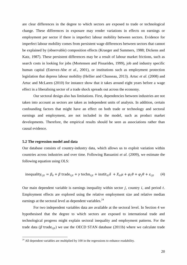
5.2 The regression model and data

Our database consists of country-industry data, which allows us to exploit variation within

countries across industries and over time. Following Bassanini et al. (2009), we estimate the

following equation using OLS:

(4)

Our main dependent variable is earnings inequality within sector , country , and period .

Employment effects are explored using the relative employment size and relative median

earnings at the sectoral level as dependent variables.24

For two independent variables data are available at the sectoral level. In Section 4 we

hypothesised that the degree to which sectors are exposed to international trade and

technological progress might explain sectoral inequality and employment patterns. For the

trade data ( ) we use the OECD STAN database (2011b) where we calculate trade

24

All dependent variables are multiplied by 100 in the regressions to enhance readability.

21

values in percentage of sectoral added value from the same year as the LIS waves. We

differentiate between import and export. Unfortunately no distinction is possible between

trade among developed and trade between developed and developing countries.25

For our

sectoral indicator of technological progress ( ) we follow OECD (2011a) and

Michaels et al. (forthcoming) and use the share of compensation of ICT capital in total capital

compensation from EU-KLEMS (2011), to which we refer to as the ICT propensity or

intensity. This indicator should be seen as an imperfect proxy to gauge technological change,

as technological change exhibits itself in multiple fashions, many of which are unobservable

(Oesch and Menés, 2011; OECD, 2011a). Further, Michaels et al. remark that the sectoral

EU-KLEMS indicator suffers from measurement error.

To test the waning labour market institutions hypothesis, we add a vector of

institutional variables at the country level ( ).26

We take a measure of overall EPL

from OECD data (2009). Visser (2011) provides us with data on union coverage, defined as

the proportion of employees covered by wage bargaining agreements, and the level of wage

coordination, where a higher number indicates a more centralised level of wage bargaining.27

The vector contains two common control variables measured at the country level,

namely, the unemployment rate and real GDP per capita divided by 100, from the OECD

National Accounts (2012). The relationship between GDP per capita and inequality is strongly

contested in both causal directions (see e.g., Thewissen, 2012) but it corrects for effects from

possible differences in economic development between countries. Inclusion of the country-

level unemployment rate can be seen as a rough control for labour market efficiency

differences between countries.

We also implicitly control for unobserved industry-specific developments by including

interactions of sector dummies and the trend ( ), such as for the fact that industries might

be exposed to different demand dynamics in their product markets. The set ( ) includes

interaction terms of the country dummies and the trend, to control for unobserved effects that

25

This is a common problem in the current literature (Bensidoun et al., 2011). As the largest increases in trade

during the last two decades came from trade between developed and developing countries, in particular, from

trade with China and India (OECD, 2011a), we conduct sensitivity tests in which we only incorporate the periods

from 1995 onwards, which does not affect the main results, see Section 5.6. 26

As a sensitivity test, we also generate interactions between the country-level labour market variables and the

sectoral indicators for import, export, and technological progress. These interactions do not reach significance,

see section 5.6 27

The variable WCoord from Visser (2011) is divided into: 5 = economy-wide bargaining, 4 = mixed industry-

and economy-wide bargaining, 3 = industry-level bargaining with no (standard) pattern setting, 2 = mixed

industry- and firm-level bargaining, 1 = fragmented or no bargaining.

22

have comparable effects on earnings within different industries at the country level.28

Standard errors are clustered at the country level to allow for general forms of

heteroskedasticity and autocorrelation within countries.

5.3 Descriptive statistics for the independent variables

Table 7 shows that the amount of import and export has increased in every sector. The largest

increase took place in the manufacturing of textile and manufacturing of transport; in mining

import rose significantly while exports remained stable. The amount of international trade

barely rose in the utility sector. As is evident from the table, for international trade data are

only available for agriculture, mining, utilities, and manufacturing and its subsectors.

Table 7 Trends in international trade and technological change at the sectoral level

Import

(% sectoral value added)

Export

(% sectoral value added)

Share of ICT in total capital

compensation

(%)

1985 1995 2005 1985 1995 2005 1985 1995 2005

1 Agriculture 21.15a 33.15 47.85 22.57a 21.43 25.81 0.19 0.02 0.03

2 Mining 285.94a 223.97 459.81 46.72a 35.01 49.97 0.03 0.05 0.11

3 Manufacturing 91.63 114.36 144.40 88.25 132.12 167.30 0.10 0.09 0.12

4 Utilities 3.13a 2.23 3.79 1.06a 1.30 5.47 0.04 0.05 0.05

5 Construction . . . . . . 0.06 0.28 0.12

6 Wholesale . . . . . . 0.19 0.16 0.18

7 Transport and

telecommunications . . . . . . 0.23 0.20 0.26

8 Finance . . . . . . 0.09 0.10 0.12

9 Community . . . . . . 0.14 0.16 0.18

31 Man. food 50.75 57.56 81.07 59.80 100.24 83.18 0.07 0.07 0.09

32 Man. textile 208.18 249.14 503.79 95.18 161.39 264.39 0.07 0.07 0.13

33 Man. wood 65.16 73.67 83.37 72.08 86.08 81.69 0.08 0.06 0.07

34 Man. paper 31.15 58.10 54.91 64.57 87.59 83.03 0.14 0.13 0.16

35 Man. chemicals 130.61 135.74 166.18 96.18 131.70 188.81 0.06 0.06 0.09

36 Man. minerals 41.20 44.93 65.52 30.37 55.16 63.09 0.09 0.07 0.07

37 Man. metals 87.43 111.04 123.94 72.77 95.02 111.63 0.07 0.08 0.13

38 Man. machinery 124.23 177.30 209.20 109.38 181.77 239.74 0.16 0.14 0.17

39 Man. transport 174.15 269.00 424.87 120.47 171.65 245.23 0.26 0.13 0.20

30 Other man. 75.77 87.87 132.52 66.65 95.82 110.70 0.09 0.12 0.26

71 Transport . . . . . . 0.13 0.14 0.15

72 Telecommunications . . . . . . 0.30 0.29 0.40

Average 99.32 117.00 178.66 67.57 96.88 122.86 0.12 0.12 0.15

Note: Import and export are expressed in % of sectoral value added, pooled for countries for which data are available.

a Data from 1990. The average is the unweighted arithmetic average for the available observations of that period.

Source: Import and export from OECD STAN, share of ICT in total capital compensation from EU-KLEMS.

The ICT propensity rose over time as well, but not uniformly across all sectors. The starkest

increases took place in other manufacturing, telecommunications, and mining. The ICT

propensity decreased significantly in agriculture, which is fully due to high values in

28

As a sensitivity test we also exclude these sets of interaction terms. These results, prone to unobserved

heterogeneity, change the results to some extent, see Section 5.6.

23

Germany around 1985.29

Minor reductions occurred in the manufacturing of wood, minerals,

and transport. As can also be seen in Table 7, for a number of sectors no data on international

trade are available. Of particular importance are the community sector, which can be expected

to be relatively sheltered against international trade, and the financial sector, in which the

relative employment size grew relatively fast.30

Table 8 summarises the country-level data for the incorporated set of institutions per

country. On average the union coverage rate decreased and EPL became less strict. Finland

and Sweden are the only countries in which the union coverage rate increased over time. In

the UK and Ireland EPL became more strict, but only marginally so. There is not much

fluctuation in the level of wage coordination within countries over time. In Sweden wage

coordination became more decentralised whereas it became more centralised in Denmark.31

Table 8 Trends in institutions at the country level

Country Union coverage rate (%) Level of wage coordination EPL

1985 1995 2005 1985 1995 2005 1985 1995 2005

Czech Republic . 60.0 43.5 . 2 2 . 1.90 1.90

Denmark 83.0 84.0 83.0 3 3 4 2.40 1.50 1.50

Finland 77.0 82.2 90.0 4 3 4 2.33 2.16 2.02

Germany 78.0 72.0 64.3 4 4 4 3.17 3.09 2.12

Ireland . 60.0 54.6 . 5 5 . 0.93 1.11

Sweden 85.0 94.0a 94.0 4 3 a 3 3.49 2.24 a 2.24

UK 64.0 36.1 34.7 1 1 1 0.60 0.60 0.75

US 19.9 17.4 13.8 1 1 1 0.21 0.21 0.21

Average 65.9 63.2 59.7 2.8 2.8 3.0 1.88 1.58 1.48

Note: a Data from around 2000. The average is the unweighted arithmetic average for the available observations of that

period.

Source: Union coverage and level of wage coordination from Visser (2011), EPL from OECD EPL

5.4 Within-industry inequality

We start with simple scatterplots for the sectoral data to examine the correlation between

changes in the first order corrected Gini coefficient and sectoral levels of import, export, and

the share of ICT. There is a weak positive relation between changes in import and the first

order corrected Gini index, as can be seen from Figure 5. For export the relationship is

marginally stronger and negative. These two signs correspond to Mahler’s (2004) predictions.

29

These extreme values for Germany drop out in the regressions as no data on export and import are available

for 1985 and 1990. 30

In Section 5.6 we make an explicit comparison between the community and the manufacturing industry for our

three dependent variables. In addition, we impute zero’s for international trade in the community sector and run

the regressions. Both analyses fully correspond to our presented findings. 31

In 1991 the Swedish Federation of Employers withdrew from the tripartite negotiations, so that the central

collective wage negotiations came to a halt (Lindvall and Sebring, 2005). In Denmark Anthonsen et al. (2010)

describe a revival of corporatism during the 1980s and 1990s.

24

There is a somewhat stronger positive association for changes in the share of ICT, which is in

line with the SBTC hypothesis.

Figure 5 OLS associations for import, export, ICT, and sectoral earnings inequality

Note: Changes in first order corrected Gini index. Differences between 1985 and 2005 for sectoral observations, except

for Czech Republic, Ireland, and Germany for import (between 1995 and 2005), and Sweden (between 2000 and

2005)

Source: First order corrected Gini index from the Leiden LIS Sectoral Income Inequality Dataset, import from OECD

STAN, share of ICT in total capital compensation from EU-KLEMS

As shown in Table 9 no evidence is found for the hypothesis that international trade leads to

higher earnings inequality at the sectoral level. The only borderline significant result is the

negative association between export and the first order corrected Gini index, which suggests

that sectors more exposed to export actually have a more compressed earnings structure.

y = 2.9*10-5x + 0.017

R² = 0.005

-0.20

-0.15

-0.10

-0.05

0.00

0.05

0.10

0.15

0.20

-200 0 200 400 600 800 1,000

Ch

an

ges

in

Gin

i in

dex

wit

hin

in

du

stri

es

Changes in import (% sectoral value added)

y = -1.12*10-4x + 0.024

R² = 0.024 -0.25

-0.20

-0.15

-0.10

-0.05

0.00

0.05

0.10

0.15

0.20

-200 0 200 400 600

Ch

an

ges

in

Gin

i in

dex

wit

hin

in

du

stri

es

Changes in export (% sectoral value added)

y = 7.72*10-2x + 0.023

R² = 0.038

-0.25

-0.20

-0.15

-0.10

-0.05

0.00

0.05

0.10

0.15

0.20

-1.00 -0.50 0.00 0.50 1.00

Ch

an

ges

in

Gin

i in

dex

wit

hin

in

du

stri

es

Changes in share of ICT

25

The sectoral ICT propensity is insignificant in all regressions, thus, we do not find

evidence for the SBTC hypothesis. The union coverage rate is consistently significant,

however, and its sign corresponds to our hypothesis that a weaker trade union position goes

hand-in-hand with a more dispersed earnings distribution. The level of wage coordination is

significant only for the Gini index regressions, whereas EPL becomes significant in the

regressions with the MLD as the dependent variable. Finally, the unemployment rate at

country level has a negative association with sectoral inequality. A possible explanation for

this is that when the unemployment rate is rampant, people with earnings at the lower end of

the distribution are most prone to job loss resulting in lower earnings inequality. Another

reason is that starters with relatively low earnings postpone entry into the labour market (e.g.,

Elsby et al., 2010).

Table 9 Panel data regressions for earnings inequality within sectors

First order corrected Gini

index

Mean log deviation

Sectoral data (1) (2) (3) (4)

Import -0.002 -0.000

(0.319) (0.797)

Export -0.008* -0.009

(0.077) (0.202)

Share of ICT 1.068 0.359 0.903 0.544

(0.553) (0.869) (0.737) (0.848)

Country level data

Union coverage -0.134*** -0.134*** -0.257*** -0.254***

rate (0.001) (0.001) (0.004) (0.003)

Level of wage -1.884*** -1.784*** -1.391 -1.288

coordination (0.001) (0.002) (0.126) (0.156)

EPL 0.897 0.912 3.478** 3.447***

(0.376) (0.343) (0.012) (0.009)

Unemployment -0.410*** -0.392*** -0.235* -0.218*

rate (0.000) (0.001) (0.071) (0.097)

Real GDP per -0.026** -0.027** -0.044 -0.045

capita/100 (0.045) (0.035) (0.124) (0.122)

Constant

44.054***

44.071***

38.350***

38.261***

(0.000) (0.000) (0.001) (0.001)

N*T*I 334 334 334 334

Adjusted R2 0.627 0.629 0.407 0.409

Note: OLS with country*period and sector*period fixed effects, full sample, 1985-2005, clustered standard errors.

Significance levels are noted by *** (1 per cent), ** (5 per cent), or * (10 per cent)

Source: First order corrected Gini index and MLD from the Leiden LIS Sectoral Income Inequality Dataset, import and

export from OECD STAN, share of ICT in total capital compensation from EU-KLEMS, union coverage and level

of wage coordination from Visser (2011), all other data from OECD

26

5.5 Employment effects

It might be that increased income inequality at country level is not so much a consequence of

widening earnings distribution, but rather of employment loss at the bottom end of the

earnings distribution (Gottschalk and Smeeding, 1997; Atkinson, 2003). As explained earlier,

unfortunately the LIS database is a time series rather than a panel at the individual level. This

makes it impossible to directly track employment shifts, such as transfers to less exposed

sectors or to unemployment.

There are two indirect measures at our disposal to map employment effects. First, we

can use data on the relative employment size of a sector. If our independent variables are

associated with job loss, we should expect a decrease in the relative employment size of the

sector. Second, if this job loss mainly occurred for people at the lower end of the earnings

distribution, we should expect higher relative median earnings in sectors that were more

exposed to trade or that were more skill-intensive (see also Mahler et al., 1999, who coin this

inequality between sectors).

For the relative employment size we use our own LIS and the OECD STAN data,

defined as the number of persons engaged per industry divided by the total number of persons

engaged. This indicator only tells us something about the extensive margin; cuts in working

hours are not incorporated. The indicators from the two data sources are highly correlated

(0.96). For the relative median earnings we divide the sectoral median earnings by its country-

level counterpart of the same period.

As both employment indicators are expressed in percentages relative to the national

level, the institutional and control variables at the country level lose their interpretation. As

the sectoral terms are expressed in ratios, they average out to around 100 at the country level.

The country-level variables are therefore left out of the regressions, although the results are

not affected by their inclusion.32

Figure 6 shows a weak negative association between changes in import, export, and

the ICT propensity on the one hand, and the relative employment size on the other. Yet, the

explanatory power is limited as evident from the low R2 value.

32

The coefficients for the country-level indicators are still estimated as for some sectors data are missing, so that

the problem of perfect collinearity does not arise.

27

Figure 6 OLS associations for import, export, ICT, and relative employment size

Note: Changes in relative employment size. Differences between 1985 and 2005 for sectoral observations, except for

Czech Republic, Ireland, and Germany for import (between 1995 and 2005), and Sweden (between 2000 and 2005)

Source: Relative employment size from the Leiden LIS Sectoral Income Inequality Dataset, import from OECD STAN,

share of ICT in total capital compensation from EU-KLEMS

We can see from the results in Table 10 that import is significantly associated with the

relative employment size of industries. We can infer from this that the relative number of jobs

has decreased in sectors more exposed to import. This is in line with the hypothesis that trade

leads to job loss in import-competing sectors. From the results we can conclude that for a

given sector, an increase in import of 1 percentage point of the sectoral value added is on

average associated with an in between 0.001 and 0.002 percentage point lower relative

employment size in a period, holding constant the control variables.

The results provide no evidence for job creation in sectors with a large export fraction.

For the ICT propensity we only find one borderline significant result; the positive direction is

y = -6*10-6x - 0.009

R² = 0.001 -0.10

-0.05

0.00

0.05

-200 0 200 400 600 800 1,000

Ch

an

ges

in

sh

are

of

rela

tive

emp

loy

men

t

size


y = -1.1*10-5x - 0.008

R² = 0.001 -0.10

-0.05

0.00

0.05

-200 0 200 400 600

Ch

an

ges

in

sh

are

of

rela

tive

emp

loy

men

t

size


y = -1.54*10-2x - 0.003

R² = 0.009 -0.20

-0.15

-0.10

-0.05

0.00

0.05

0.10

-1.00 -0.50 0.00 0.50 1.00Ch

an

ges

in

sh

are

of

rela

tive

emp

loy

men

t

size

Changes in share of ICT in total capital

compensation

28

not in agreement with the SBTC job loss hypothesis. The fact that we find a decline in

employment in import-competing industries combined with no significant association with

technological progress is in line with the industrial findings from Autor et al. (2013) for the

US.

Table 10 Panel data regressions for the relative employment size

LIS data OECD data


Import -0.002*** -0.001***

(0.007) (0.005)

Export 0.001 -0.001

(0.232) (0.673)

Share of ICT 0.686* 0.386 0.434 0.125

(0.097) (0.377) (0.207) (0.730)

Constant

2.660***

2.611***

2.215***

2.224***

(0.000) (0.000) (0.000) (0.000)

N*T*I 334 334 339 339

Adjusted R2 0.627 0.609 0.672 0.655



Source: Relative employment size from OECD STAN and Leiden LIS Sectoral Income Inequality Dataset, import and

export from OECD STAN, share of ICT in total capital compensation from EU-KLEMS

Yet, the relative employment size does not necessarily tell us something about job loss for

lowly skilled; it simply captures all relative job movements. Therefore, we also use the

sectoral median earnings relative to the national median earnings. In case that low wage jobs

for lowly skilled have disappeared we should expect higher relative median earnings in

sectors that became more exposed to international trade or more skill intensive.

Figure 7 shows that the OLS associations are generally weak. Changes in both import

and export have a marginal positive association with changes in the relative median earnings.

This positive sign corresponds to the hypothesis that trade leads to job loss at the lower end of

the distribution, resulting in higher relative median earnings. For the ICT propensity a

somewhat stronger negative association is reported.

29

Figure 7 OLS associations for import, export, ICT, and relative median earnings

Note: Differences between 1985 and 2005 for sectoral observations, except for Czech Republic, Ireland, and Germany for

import (between 1995 and 2005), and Sweden (between 2000 and 2005)

Source: Relative median earnings from the Leiden LIS Sectoral Income Inequality Dataset, import from OECD STAN,

share of ICT in total capital compensation from EU-KLEMS

The regressions presented in Table 11 actually show a negative association between import

and the relative median earnings which is significant at the 10 per cent level. This finding

indicates that the diminution of employment found in the former regressions is not associated

with concomitant job loss for the lowly skilled, although the evidence is not particularly

strong here. All things considered, we find that sectors more exposed to import are

characterised by a lower number of jobs, potentially lower median earnings, but not a more

dispersed earnings distribution. An explanation for this is that job loss in import-competing

sectors is not only tailored to the low end of the earnings distribution, but rather that the

whole distribution shifts down as a result of increased international competition. Other

y = 3.5*10-5x + 0.016

R² = 0.002 -0.40

-0.30

-0.20

-0.10

0.00

0.10

0.20

0.30

0.40

0.50

0.60

-200 0 200 400 600 800 1,000

Ch

an

ges

in

rel

ati

ve

med

ian

earn

ing

s


y = 1.6*10-5x + 0.017

R² = 0.0001 -0.40

-0.30

-0.20

-0.10

0.00

0.10

0.20

0.30

0.40

0.50

0.60

-200 0 200 400 600

Ch

an

ges

in

rel

ati

ve

med

ian

earn

ing

s


y = -1.54*10-1x + 0.027

R² = 0.035 -0.40

-0.30

-0.20

-0.10

0.00

0.10

0.20

0.30

0.40

0.50

0.60

-1.00 -0.50 0.00 0.50 1.00

Ch

an

ges

in

rel

ati

ve

med

ian

earn

ing

s

Changes in share of ICT in total capital

compensation

30

explanations are feasible as well though, and in addition, the evidence for lower relative

median earnings is weak. For export and ICT intensity no significant associations are

reported.

Table 11 Panel data regressions for the relative median earnings

Relative median earnings

Sectoral data (1) (2)

Import -0.016*

(0.054)

Export

0.014

(0.516)

Share of ICT 3.596 0.485

(0.713) (0.962)

Constant

103.335***

102.721***

(0.000) (0.000)

N*T*I 334 334

Adjusted R2 0.660 0.650



Source: Relative median earnings from the Leiden LIS Sectoral Income Inequality Dataset, import and export from OECD

STAN, share of ICT in total capital compensation from EU-KLEMS

5.6 Sensitivity tests

We perform a battery of additional tests to examine the sensitivity of our findings, results of

which are placed in Appendix 1. First, we test whether the reported results are sensitive to the

selected sample. We exclude the industries in which the number of included individuals in the

LIS data is below 30, causing the number of observations to decrease from 334 to 316. This

does not affect the results, see Table A1.1. Second, we test for the possibility that trade only

had an effect from around 1995 onwards, when the trade between developed and developing

countries mainly increased (OECD, 2011a). As can be seen in Table A1.2, this alters the

regressions with sectoral earnings inequality as the dependent variable somewhat; export

becomes insignificant and so does the union coverage rate for the MLD, whereas the level of

wage coordination and EPL become significant in all regressions.

In our original results the community sector was excluded as no data for international

trade are available. If we compare trends in earnings inequality and employment in the

community and manufacturing sector per country, then we find that earnings inequality is

actually higher and more rapidly rising in the sheltered community sector, which again does

not suggest inequality-enhancing effects of international trade (see Table 12a). Yet, we can

see that the relative employment size decreased more quickly in the manufacturing industry

31

combined with increasing relative median earnings (Tables 12b and 12c). This hints to

possible employment effects of international trade.

Table 12 Comparing the manufacturing and the community sector

12a First order corrected Gini index

Country Manufacturing Community

1985 1990 1995 2000 2005 Change 1985 1990 1995 2000 2005 Change

1. Czech Rep. . . 0.305 . 0.293 -0.012 . . 0.266 . 0.285 0.019

2. Denmark 0.235 0.225 0.230 0.222 0.238 0.003 0.254 0.259 0.239 0.237 0.254 -0.001

3. Finland 0.232 0.239 0.222 0.246 0.243 0.011 0.262 0.262 0.255 0.258 0.249 -0.013

4. Germany 0.295 0.279 0.290 0.294 0.305 0.010 0.295 0.304 0.321 0.327 0.354 0.059

5. Ireland . . 0.269 . 0.300 0.031 . . 0.273 . 0.356 0.084

6. Sweden 0.266 0.251 . 0.254 0.249 -0.017 0.282 0.293 . 0.288 0.295 0.013

7. UK 0.286 . . 0.337 0.326 0.040 0.363 . . 0.389 0.372 0.009

8. US 0.331 0.340 0.363 0.377 0.378 0.048 0.372 0.388 0.399 0.409 0.397 0.025

Average 0.274 0.267 0.280 0.288 0.291 0.014 0.305 0.301 0.292 0.318 0.320 0.024

12b Relative employment size


1985 1990 1995 2000 2005 Change 1985 1990 1995 2000 2005 Change

1. Czech Rep. . . 0.270 . 0.264 -0.006 . . 0.317 . 0.246 -0.072

2. Denmark 0.180 0.185 0.189 0.179 0.165 -0.015 0.422 0.438 0.377 0.372 0.399 -0.023

3. Finland 0.243 0.219 0.224 0.220 0.206 -0.037 0.284 0.312 0.342 0.307 0.328 0.045

4. Germany 0.351 0.364 0.263 0.255 0.254 -0.097 0.270 0.253 0.298 0.294 0.312 0.041

5. Ireland . . 0.194 . 0.126 -0.068 . . 0.358 . 0.332 -0.026

6. Sweden 0.215 0.190 . 0.194 0.181 -0.034 0.406 0.419 . 0.388 0.406 -0.001

7. UK 0.291 . . 0.197 0.147 -0.144 0.350 . . 0.318 0.353 0.003

8. US 0.201 0.196 0.186 0.161 0.131 -0.069 0.331 0.312 0.331 0.321 0.319 -0.013

Average 0.247 0.231 0.221 0.201 0.184 -0.059 0.344 0.347 0.337 0.333 0.337 -0.006

12c Relative median earnings


1985 1990 1995 2000 2005 Change 1985 1990 1995 2000 2005 Change

1. Czech Rep. . . 0.938 . 0.951 0.013 . . 1.018 . 1.062 0.044

2. Denmark 1.061 1.052 1.042 1.031 1.049 -0.012 0.914 0.930 0.960 0.959 0.950 0.036

3. Finland 1.066 1.059 1.143 1.146 1.129 0.062 0.993 1.010 0.966 0.926 0.946 -0.048

4. Germany 1.046 1.053 1.129 1.143 1.167 0.121 0.991 0.969 0.966 0.969 0.922 -0.068

5. Ireland . . 0.926 . 1.011 0.085 . . 1.093 . 1.043 -0.050

6. Sweden 1.075 1.079 . 1.118 1.119 0.044 0.888 0.914 . 0.890 0.902 0.014

7. UK 1.088 . . 1.110 1.106 0.018 0.908 . . 0.907 0.941 0.033

8. US 1.123 1.152 1.116 1.133 1.100 -0.023 0.963 0.991 0.983 1.000 0.970 0.007

Average 1.077 1.079 1.049 1.114 1.079 0.039 0.943 0.963 0.998 0.942 0.967 -0.004

Note: The average is the unweighted arithmetic average for the available observations of that period


Comparable results are obtained if we assume that no trade took place in the community

sector by replacing the zeros for missing values and redoing the estimations, see Table A1.3

(the N increases to 363). Compared to the original regression results, the only difference is

that export becomes insignificant for the first order corrected Gini index.

Next, we test more generally whether the reported results are robust to the exclusion of

sectors. The general picture is again confirmed; import remains significantly associated with

32

the relative employment size, as can be seen from Figure A1.1. The coefficient becomes twice

as strong (-0.003 for both LIS and OECD data) when the mining sector is excluded. The

significant association between the union coverage rate and earnings inequality is also robust

to the exclusion of sectors, see Figure A1.2. The significant associations between export and

the first order corrected Gini coefficient and between import and relative median earnings

disappear frequently (results not shown).

Subsequently, the fact that we do not find many significant results might be due to the

conservative nature of our empirical specification. By including interactions of country

dummies and the time trend, or sector dummies and the time trend, we remove patterns over

time in sectors and countries from the data which reduces the variation. Therefore we also

estimate the models without the dummies, see Tables A1.4-A1.6. This comes at a high price

though, as it makes the results more susceptible to unobserved heterogeneity bias. There are

still no signs of inequality-enhancing effects of international trade. Without the country and

time trend interactions the institutions become significant in all four inequality regressions.

There are some signs of a significant positive association between export and the relative

employment size, entailing that export could lead to job creation, when the sector and time

trend interactions are removed. The initially found negative significant association between

import and the relative median earnings disappears regularly.

One way to cope with the fact that we do not have sectoral information for the labour

market institution variables is to calculate interactions between the sectoral indicators (import,

export, and technological change) and the three labour market institutions (EPL, level of wage

coordination, and the union coverage rate). In this way we test whether the effects of

international trade or technological change on earnings inequality at the sectoral level are

mitigated through the country-level labour market institutions. None of the interaction

variables in the regressions with earnings inequality as the dependent variable reach

significance, both with and without the original institution and sectoral variables included.

The results for the regressions including all interactions are shown in Table A1.7.

It could be that parts of the changes in earnings or employment are caused by people

shifting from unemployment to part-time unemployment or from part-time to fulltime jobs.

Especially spouses and other relatives are prone to make these labour shifts. We recalculate

all indicators for household heads only33

and redo the regressions, see Table A1.8;

correlations with the original indicators are above 0.94 for the sectoral earnings inequality and

33

These indicators are also included in the database.

33

employment size, and 0.85 for the relative median earnings. There are still no signs of

inequality-enhancing effects of international trade, while EPL becomes significantly positive

for the first order corrected Gini index. The association between the relative sectoral size and

import remains firm, whereas the significance between import and the relative median

earnings disappears.

Last, we explore possible consequences of the fact that we base our estimations on

individual rather than household earnings, as Mahler et al. (1999) did. Employing household

earnings introduces noise into the dataset as earnings are attributed to sectors in which they

were not necessarily made. However, if labour supply decisions are made at the household

level and when earnings are shared between household members, it might be preferable to

base the regressions on household data.34

The correlations between the individual and

household data indicators are high for the relative employment size (above 0.93), but lower

for the inequality indicators (0.82 for the first order corrected Gini index and 0.67 for the

MLD) and the relative median earnings (0.68). As can be seen from Table A1.9, we still do

not find evidence for inequality-enhancing effects from international trade, whilst the level of

wage coordination becomes comfortably significant for all regressions. The most salient

finding is the robustly significant positive association between the ICT propensity and within-

sector inequality. Thus, based on household level data we do find evidence for SBTC. The

employment regressions correspond to the ones based on individual data, except the

consistently insignificant association between trade and relative median earnings that was

already apparent from the other sensitivity tests.

6. Conclusions

This paper describes trends in sectoral labour earnings inequality and employment using a

new database containing information for eight countries between 1985 and 2005. In addition,

using cross-sectional pooled time-series we scrutinise possible explanations for variations in

sectoral inequality and employment.

Our decomposition divulges that earnings inequality at the country level is by and

large a consequence of dispersion within sectors rather than large differences in mean

earnings between sectors. This share of within-sector inequality has increased further over

time. Having said that, the level of sectoral earnings inequality within countries fluctuates as

much as the level of earnings inequality between countries. The ranking of sectors in their

34

These indicators are also included in the database.

34

level of inequality is comparable across countries, indicating that the sectoral dimension is

important for understanding earnings inequality at the country level. Agriculture, wholesale,

and the financial sector ubiquitously stand out as the sectors with the most unequally

distributed earnings, whereas mining, utilities, and the manufacturing of metals and transport

are characterised by low levels of earnings dispersion in all countries.

Mirroring the developments at the country level, earnings inequality has increased in

the lion’s share of sectors, although the rise differs per sector. In the sector with the highest

level of inequality, agriculture, there is in fact a trend towards equalisation over time. The

mining and utilities industries comprise a relatively homogeneous workforce as they are

characterised by a relatively even earnings distribution, combined with relatively high median

earnings. The median earnings are relatively low in the traditionally labour-intensive

industries, namely, agriculture, wholesale, and the manufacturing of textile, although median

earnings are rising fast in the agricultural sector. It thus seems that in agriculture individuals

at the lower end of the earnings distribution saw an increase in their earnings, as indicated by

an increase in relative median earnings combined with a decrease in earnings inequality. Our

comparison of the relative employment sizes of industries over time imparts a notable

employment shift from the manufacturing industry towards the financial sector. For all these

trends the differences across countries are limited.

By means of cross-sectional pooled time-series we do not find evidence for

associations between trade and earnings inequality, in line with other sectoral studies (Mahler

et al., 1999; OECD, 2011a; Michaels et al., forthcoming). Yet, the reported results denote that

the employment size has decreased in sectors that are more exposed to import. No further

evidence is found that this job loss has occurred at the bottom end of the earnings distribution.

In addition, the union coverage rate at the country level is found to be negatively associated

with sectoral earnings inequality, which corresponds to the hypothesis that waning trade union

power is an explanation for rising inequality (e.g., Koeniger et al., 2007). These results are

robust to a set of sensitivity analyses. Further inspection using sectoral data on union coverage

rates could provide more insight into how trade unions’ influence works its way into sectoral

earnings differences.

The regression results are not in line with the predictions from the SBTC hypothesis,

as we do not find significant associations between the sectoral ICT intensity and any of the

dependent variables. In particular from the wage literature there is empirical support the

SBTC hypothesis. A first reason for this difference is imperfect measurement; sectoral proxies

for technological change are not abundantly available and they suffer from measurement

35

error. The deviation from Michaels et al. (forthcoming) might arise from the fact that these

scholars examine polarisation in skill demand, rather than earnings inequality, and that they

only use two periods over time. It therefore might be interesting to further analyse in what

way polarisation seeps through to inequality at the sectoral level.

The conducted regressions do not provide causal evidence. Other confounding factors,

in particular in product markets, can be expected to affect both the earnings and employment,

as well as the trade and technology. In addition, individual labour market transitions cannot be

tracked directly by means of the used database. Still, the analyses instigate a sectoral approach

in understanding inequality, in which heterogeneity between sectors is accounted for.

36

References

Acemoglu, D. (2003a) ‘Patterns of Skill Premia’, Review of Economic Studies, 70, 199-230.

Acemoglu, D. (2003b) ‘Cross-Country Inequality Trends’, The Economic Journal, 113, F121-

F149.

Alderson, A. and Nielsen, F. (2002) ‘Globalization and the Great U-Turn: Income Inequality

Trends in 16 OECD Countries’, American Journal of Sociology, 107, 1244-1299.

Anthonsen, M., Lindvall, J., and Schmidt-Hansen, U. (2010) ‘Social Democrats, Unions and

Corporatism: Denmark and Sweden Compared’, Party Politics, 17, 118-134.

Artuc, E., Chaudhuri, S., and McLaren, J. (2008) ‘Delay and Dynamics in Labor Market

Adjustment: Simulation Results’, Journal of International Economics, 75, 1-13.

Artuc, E. and McLaren, J. (2010) ‘A Structural Empirical Approach to Trade Shocks and

Labor Adjustment: An Application to Turkey’. In Hoekman, B. and Porto, G. (eds) Trade

Adjustment Costs in Developing Countries: Impacts, Determinants and Policy Responses,

Washington DC, The World Bank.

Atkinson, A. (1970) ‘On the Measurement of Inequality’, Journal of Economic Theory, 2,

244-263.

Atkinson, A. (2003) ‘Income Inequality in OECD Countries: Data and Explanations’, CESifo

Economic Studies, 49, 479-513.

Atkinson, A., Piketty, T., and Saez, E. (2011) ‘Top Incomes in the Long Run of History’,

Journal of Economic Literature, 1, 3-71.

Atkinson, A., Rainwater, L., and Smeeding, T. (1995) ‘Income Distribution in OECD

Countries: Evidence from the Luxembourg Income Study’, OECD Social Policy Studies,

18.

Autor, D., Levy, F., and Murnane, R. (2003) ‘The Skill Content of Recent Technological

Change: An Empirical Exploration’, The Quarterly Journal of Economics, 118, 1279-

1333.

Autor, D., Katz, L., and Kearney, M. (2006) ‘The Polarization of the U.S. Labor Market’,

American Economic Review, 92, 189-194.

Autor, D., Dorn, D., and Hanson, G. (2013) ‘Untangling Trade and Technology : Evidence

from Local Labor Markets’, IZA Discussion Paper, 7329.

Bassanini, A., Nunziata, L. and Venn, D. (2009) ‘Job Protection Legislation and Productivity

Growth in OECD Countries’, Economic Policy, 24, 349-402.

Bensidoun, I., Jean, S., and Sztulman, A. (2011) ‘International Trade and Income

Distribution: Reconsidering the Evidence’, Review of World Economics, 147, 593-619.

37

Bergh, A. and Nilsson, T. (2010) ‘Do Liberalization and Globalization Increase Income

Inequality?’, European Journal of Political Economy, 26, 488-505.

Brandolini, A. and Smeeding, T. (2008) ‘Inequality Patterns in Western Democracies: Cross-

Country Differences and Changes over Time’. In Beramandi, P. and Anderson, C. (eds)

Democracy, Inequality, and Representation, New York, The Russell Sage Foundation, 25-

61.

Brandolini, A. and Smeeding, T. (2009) ‘Income Inequality in Richer and OECD Countries’.

In Salverda, W., Nolan, B. and Smeeding, T. (eds.) The Oxford Handbook of Economic

Inequality, Oxford, Oxford University Press, 71-100.

Caminada, K., Goudswaard, K., and Wang, C. (2012) ‘Disentangling Income Inequality and

the Redistributive Effect of Taxes and Transfers in 20 LIS Countries Over Time’, LIS

Working Paper Series, 581.

Checchi, D. and García-Peñalosa, C. (2008) ‘Labour Market Institutions and Income

Inequality’, Economic Policy, 23, 601-649.

Cowell, F. and Fiorio, C. (2011) ‘Inequality Decompositions: A Reconciliation’, Journal of

Economic Inequality, 9, 509-528.

Davis, D. and Mishra, P. (2007) ‘Stolper-Samuelson Is Dead - and Other Crimes of Both

Theory and Data’. In Harrison, A. (ed) Globalization and Poverty, Chicago, University of

Chicago Press, 87-107.

Deltas, G. (2003) ‘The Small-Sample Bias of the Gini Coefficient: Results and Implications

for Empirical Research’, The Review of Economics and Statistics, 85, 226-234.

Dickens, W. and Katz, L. (1987) ‘Interindustry Wage Differences and Industry

Characteristics’, NBER Working Paper, 2014.

Dreher, A. and Gaston, N. (2008) ‘Has Globalization Increased Inequality?’, Review of

International Economics, 16, 516-536.

Dustmann, C., Ludsteck, J., and Schonberg, U. (2009) ‘Revisiting the German Wage

Structure’, The Quarterly Journal of Economics, 124, 843-881.

Elsby, M., Hobijn, B., and Sahin, A. (2010) ‘The Labor Market in the Great Recession’,

Brookings Papers on Economic Activity, 41, 1-69.

Estevez-Abe, M., Iversen, T., and Soskice, D. (2001) ‘Social Protection and the Formation of

Skills: A Reinterpretation of the Welfare State’. In Hall, P. and Soskice, D. (eds) Varieties

of Capitalism: The Institutional Foundations of Comparative Advantage, Oxford, Oxford

University Press, 145-183.

38

EU-KLEMS (2011) Growth and Productivity Accounts – March Update,

http://www.euklems.net/.

Förster, M. and Vleminckx, K. (2004) ‘International Comparisons of Income Inequality and

Poverty: Findings from the Luxembourg Income Study’, Socio-Economic Review, 2, 191-

212.

Freeman, R. (1995) ‘Are Your Wages Set in Beijing?’, The Journal of Economic

Perspectives, 9, 15-32.

Fuchs-Schündeln, N., Krueger, D., and Sommer, M. (2010) ‘Inequality Trends for Germany

in the Last Two Decades’, Review of Economic Dynamics, 13, 103-132.

Goos, M. and Manning, A. (2007) ‘Lousy and Lovely Jobs: The Rising Polarization of Work

in Britain’, The Review of Economics and Statistics, 89, 118-133.

Goos, M., Manning, A., and Salomons, A. (2009) ‘Job Polarization in Europe’, American

Economic Review, 99, 58-63.

Gottschalk, P. and Smeeding, T.M. (1997) ‘Cross-National Comparisons of Earnings and

Income Inequality’, Journal of Economic Literature, 35, 633-687.

Harrison, A., McLaren, J., and McMillan, M. (2011) ‘Recent Perspectives on Trade and

Inequality’, Annual Review of Economics, 3, 261-289.

Hellier, J. and Chusseau, N. (eds) (2013) Growing Income Inequalities – Economic Analyses.

New York: Palgrave Macmillan.

Immervoll, H. and Richardson, L. (2011) ‘Redistribution Policy and Inequality Reduction in

OECD Countries: What Has Changed in Two Decades?’, OECD Social, Employment and

Migration Working Papers, 122.

Kampelmann, S. (2009) ‘Inequality Measures as Conventions: New Interpretations of a

Classic Operationalization Problem’, Socio-Economic Review, 7, 679-694.

Kenworthy, L. and Pontusson, J. (2005) ‘Rising Inequality and the Politics of Redistribution

in Affluent Countries’, Perspectives on Politics, 3, 449-471.

Koeniger, W., Leonardi, M., and Nunziata, L. (2007) ‘Labor Market Institutions and Wage

Inequality’, Industrial and Labor Relations Review, 60, 340-356.

Kremer, M. and Maskin, E. (2006) ‘Globalization and Inequality’, unpublished manuscript.

Krueger, A. and Summers, L. (1988) ‘Efficiency Wages and the Interindustry Wage

Structure’, Econometrica, 56, 259-263.

Lindvall, J. and Sebring, J. (2005) ‘Policy Reform and the Decline of Corporatism in

Sweden’, West European Politics, 28, 1057-1074.

http://www.euklems.net/

39

LIS (2013) Luxembourg Income Study (LIS) Database. Micro data runs completed 1st of June

2013, www.lisdatacenter.org.

Lucifora, C., McKnight, A., and Salverda, W. (2005) ‘Low-Wage Employment in Europe: A

Review of the Evidence’, Socio-Economic Review, 3, 259-292.

Mahler, V. (2004) ‘Economic Globalization, Domestic Politics, and Income Inequality in the

Developed Countries’, Comparative Political Studies, 37, 1025-1053.

Mahler, V. and Jesuit, D. (2006) ‘Fiscal Redistribution in the Developed Countries: New

Insights from the Luxembourg Income Study’, Socio-Economic Review, 4, 483-511.

Mahler, V., Jesuit, D., and Roscoe, D. (1999) ‘Exploring the Impact of Trade and Investment

on Income Inequality: a Cross-National Sectoral Analysis of the Developed Countries’,

Comparative Political Studies, 32, 363-395.

Michaels, G., Natraj, A., and Van Reenen, J. (forthcoming) ‘Has ICT Polarized Skill

Demand? Evidence from Eleven Countries over 25 Years’, Review of Economics and

Statistics.

Mortensen, D. and Pissarides, C. (1999) ‘New Developments in Models of Search in the

Labor Market’. In Ashenfelter, O. and Card, D. (eds) Handbook of Labor Economics,

North-Holland, Elsevier, 2567-2627.

OECD (2008) Growing Unequal? Income Distribution and Poverty in OECD Countries,

Paris: OECD.

OECD (2009) Employment Database. Paris: OECD.

OECD (2011a) Divided We Stand: Why Inequality Keeps Rising, Paris: OECD.

OECD (2011b) STAN Structural Analysis Database. Paris: OECD.

OECD (2012) National Accounts. Paris: OECD.

Oesch, D. and Menés, J. (2011) ‘Upgrading or Polarization? Occupational Change in Britain,

Germany, Spain and Switzerland, 1990-2008’, Socio-Economic Review 9(3): 503-531.

Oliver, R. (2008) ‘Diverging Developments in Wage Inequality: Which Institutions Matter?’,

Comparative Political Studies, 41, 1551-1582.

Pontusson, J., Rueda, D., and Way, C. (2002) ‘Comparative Political Economy of Wage

Distribution: The Role of Partisanship and Labour Market Institutions’, British Journal of

Political Science, 32, 281-308.

Thewissen, S. (2012) ‘Is It the Income Distribution or Redistribution That Affects Growth?’,

Leiden Department of Economics Research Memorandum, 2012.01.

Van Reenen, R. (2011) ‘Wage Inequality, Technology and Trade: 21st Century Evidence’

Labour Economics, 18, 730-741.

http://www.lisdatacenter.org/

40

Van Vliet, O. (2011) Convergence and Europeanisation: The Political Economy of Social and

Labour Market Policies, dissertation, Leiden: Leiden University Press.

Visser, J. (2011) ‘ICTWSS: Database on Institutional Characteristics of Trade Unions, Wage

Setting, State Intervention and Social Pacts in 34 Countries between 1960 and 2007’,

AIAS, http://www.uva-aias.net/208.

Wang, C., Thewissen, S., and Van Vliet, O. (2013) ‘Leiden Sectoral Income Inequality

Dataset: Version 1’. Leiden University, www.hsz.leidenuniv.nl.

Winner, H. (2012) ‘Fiscal Competition and the Composition of Public Expenditure: An

Empirical Study’, Contemporary Economics, 6, 38-54.

World Bank (2012) World Development Indicators.

http://databank.worldbank.org/data/databases.aspx. Accessed 10 January 2013.

http://www.uva-aias.net/208

http://databank.worldbank.org/data/databases.aspx

41

Appendix 1. Sensitivity tests

Table A1.1 Without sectors with number of individuals below 30

A1.1a Earnings inequality: Without sectors with number of individuals below 30


index

Mean log deviation


Import -0.004 -0.005

(0.116) (0.207)

Export -0.009** -0.009

(0.026) (0.168)

Share of ICT 0.840 -0.283 1.554 0.283

(0.593) (0.884) (0.570) (0.929)

Country level data

Union coverage -0.133*** -0.132*** -0.249*** -0.249***

rate (0.000) (0.000) (0.003) (0.003)

Level of wage -1.586** -1.653*** -0.938 -1.024

coordination (0.011) (0.010) (0.310) (0.282)

EPL 1.005 1.095 3.462*** 3.567***

(0.298) (0.249) (0.003) (0.002)

Unemployment -0.302** -0.296** -0.096 -0.090

rate (0.025) (0.025) (0.514) (0.548)

Real GDP per -0.023 -0.024 -0.038 -0.038

capita/100 (0.162) (0.146) (0.218) (0.218)

Constant

42.171***

42.309***

35.179***

35.355***

(0.000) (0.000) (0.003) (0.003)

N*T*I 316 316 316 316

Adjusted R2 0.628 0.629 0.402 0.402

A1.1b Relative employment size: Without sectors with number of individuals below 30

LIS data OECD data


Import -0.003*** -0.003***

(0.006) (0.005)

Export 0.001 -0.001

(0.295) (0.649)

Share of ICT 0.987** 0.370 0.647 -0.054

(0.029) (0.373) (0.139) (0.893)

Constant

2.854***

2.732***

2.290***

2.263***

(0.000) (0.000) (0.000) (0.000)

N*T*I 316 316 307 307

Adjusted R2 0.636 0.604 0.673 0.646

42

A1.1c Relative median earnings: Without sectors with number of individuals below 30



Import -0.025*

(0.095)

Export 0.016

(0.460)


(0.597) (0.882)

Constant

103.501***

102.240***

(0.000) (0.000)

N*T*I 316 316

Adjusted R2 0.681 0.672



Source: First order corrected Gini index, MLD, relative employment size and relative median earnings from the Leiden LIS

Sectoral Income Inequality Dataset, relative employment size, import, and export from OECD STAN, share of ICT

in total capital compensation from EU-KLEMS, union coverage and level of wage coordination from Visser

(2011), all other data from OECD

Table A1.2 After and including 1995

A1.2a Earnings inequality: After and including 1995


index

Mean log deviation


Import -0.003 -0.000

(0.265) (0.790)

Export -0.008 -0.006

(0.117) (0.289)

Share of ICT 1.907 0.913 1.545 1.211

(0.260) (0.690) (0.597) (0.708)

Country level data

Union coverage -0.152*** -0.152*** -0.188 -0.186

rate (0.006) (0.004) (0.113) (0.100)

Level of wage -1.749** -1.668** -2.379* -2.326*

coordination (0.027) (0.029) (0.087) (0.091)

EPL 2.005* 1.949* 3.553** 3.472**

(0.071) (0.071) (0.033) (0.029)

Unemployment -0.414*** -0.395*** 0.012 0.022

rate (0.002) (0.004) (0.938) (0.888)

Real GDP per -0.030 -0.030* -0.019 -0.020

capita/100 (0.109) (0.092) (0.527) (0.490)

Constant

43.326***

43.480***

29.877**

30.052**

(0.000) (0.000) (0.012) (0.011)

N*T*I 260 260 260 260

Adjusted R2 0.643 0.643 0.459 0.460

43

A1.2b Relative employment size: After and including 1995

LIS data OECD data


Import -0.001*** -0.001**

(0.009) (0.013)

Export 0.000 -0.001

(0.893) (0.322)

Share of ICT 0.140 -0.269 0.255 -0.128

(0.736) (0.626) (0.503) (0.792)

Constant

2.636***

2.671***

2.179***

2.257***

(0.000) (0.000) (0.009) (0.005)

N*T*I 260 260 260 260

Adjusted R2 0.695 0.671 0.711 0.695

A1.2c Relative median earnings: After and including 1995



Import -0.016**

(0.041)

Export 0.008

(0.679)

Share of ICT 1.436 -2.870

(0.854) (0.773)

Constant

98.803***

98.899***

(0.000) (0.000)

N*T*I 260 260

Adjusted R2 0.714 0.700







44

Table A1.3

A1.3a Earnings inequality: Including the community sector


index

Mean log deviation


Import -0.002 -0.000

(0.336) (0.992)

Export -0.007 -0.006

(0.119) (0.377)

Share of ICT 0.541 -0.084 -0.363 -0.550

(0.770) (0.969) (0.901) (0.853)

Country level data

Union coverage -0.125*** -0.125*** -0.243*** -0.240***

rate (0.002) (0.001) (0.002) (0.001)

Level of wage -1.851*** -1.772*** -1.480 -1.416

coordination (0.001) (0.001) (0.110) (0.128)

EPL 0.774 0.784 3.109*** 3.078***

(0.447) (0.422) (0.006) (0.004)

Unemployment -0.380*** -0.366*** -0.208* -0.198

rate (0.000) (0.001) (0.086) (0.105)

Real GDP per -0.021* -0.022** -0.037 -0.037

capita/100 (0.056) (0.045) (0.131) (0.133)

Constant

43.050***

43.102***

37.420***

37.372***

(0.000) (0.000) (0.000) (0.000)

N*T*I 363 363 363 363

Adjusted R2 0.640 0.641 0.424 0.425

A1.3b Relative employment size: Including the community sector

LIS data OECD data


Import -0.002** -0.001**

(0.012) (0.014)

Export -0.003 -0.001

(0.112) (0.600)

Share of ICT 1.450 0.919 1.316 0.961

(0.131) (0.185) (0.155) (0.247)

Constant

5.664***

5.765***

4.157***

4.198***

(0.000) (0.000) (0.000) (0.000)

N*T*I 363 363 366 366

Adjusted R2 0.873 0.872 0.870 0.870

45

A1.3c Relative median earnings: Including the community sector



Import -0.016**

(0.050)

Export 0.011

(0.595)


(0.679) (0.926)

Constant

102.591***

102.130***

(0.000) (0.000)

N*T*I 363 363

Adjusted R2 0.657 0.647







Figure A1.1 Excluding sectors for import and the relative employment size

A1.1a Import and relative employment size LIS data (Table 10 column 1)

-0.006

-0.005

-0.004

-0.003

-0.002

-0.001

0

Agr

icu

ltu

re

Min

ing

Uti

litie

s

Man

. fo

od

Man

. tex

tile

Man

. wo

od

Man

. pap

er

Man

. ch

emic

als

Man

. min

era

ls

Man

. me

tals

Man

. mac

hin

ery

Man

. tra

nsp

ort

Oth

er m

an.

Imp

ort

co

effi

cien

t af

ter

dro

pp

ing

the

sect

or

46

A1.1b Import and relative employment size OECD data (Table 10 column 3)

Note: Regression: See Table 10. Dashed line: coefficient of import (% sectoral value added) in when all sectors are

included. Black marked line: coefficient of import when the below-mentioned sector is excluded. Grey lines: 95 per

cent confidence intervals

Source: See Table 10, relative employment size from the Leiden LIS Sectoral Income Inequality Dataset and OECD STAN,

import from OECD STAN

Figure A1.2 Earnings inequality: Excluding sectors for the union coverage rate

A1.2a First order corrected Gini index and import (Table 9 column 1)

-0.0045

-0.004

-0.0035

-0.003

-0.0025

-0.002

-0.0015

-0.001

-0.0005

0

Agr

icu

ltu

re

Min

ing

Uti

litie

s

Man

. fo

od

Man

. tex

tile

Man

. wo

od

Man

. pap

er

Man

. ch

emic

als

Man

. min

era

ls

Man

. me

tals

Man

. mac

hin

ery

Man

. tra

nsp

ort

Oth

er m

an.

Imp

ort

co

effi

cien

t af

ter

dro

pp

ing

the

sect

or

-0.25

-0.2

-0.15

-0.1

-0.05

0

Agr

icu

ltu

re

Min

ing

Uti

litie

s

Man

. fo

od

Man

. tex

tile

Man

. wo

od

Man

. pap

er

Man

. ch

emic

als

Man

. min

era

ls

Man

. me

tals

Man

. mac

hin

ery

Man

. tra

nsp

ort

Oth

er m

an.

Un

ion

co

vera

ge r

ate

coef

fici

ent

afte

r d

rop

pin

g th

e se

cto

r

47

A1.2b First order corrected Gini index and export (Table 9 column 2)

A1.2c Mean log deviation and import (Table 9 column 3)

-0.25

-0.2

-0.15

-0.1

-0.05

0

Agr

icu

ltu

re

Min

ing

Uti

litie

s

Man

. fo

od

Man

. tex

tile

Man

. wo

od

Man

. pap

er

Man

. ch

emic

als

Man

. min

era

ls

Man

. me

tals

Man

. mac

hin

ery

Man

. tra

nsp

ort

Oth

er m

an.

Un

ion

co

vera

ge r

ate

coef

fici

ent

afte

r d

rop

pin

g th

e se

cto

r

-0.5

-0.45

-0.4

-0.35

-0.3

-0.25

-0.2

-0.15

-0.1

-0.05

0

Agr

icu

ltu

re

Min

ing

Uti

litie

s

Man

. fo

od

Man

. tex

tile

Man

. wo

od

Man

. pap

er

Man

. ch

emic

als

Man

. min

era

ls

Man

. me

tals

Man

. mac

hin

ery

Man

. tra

nsp

ort

Oth

er m

an.

Un

ion

co

vera

ge r

ate

coef

fici

ent

afte

r d

rop

pin

g th

e se

cto

r

48

A1.2d Mean log deviation and export (Table 9 column 4)

Note: Regression: See Table 9. Dashed line: coefficient of the union coverage rate when all sectors are included. Black

marked line: coefficient of the union coverage rate when the below-mentioned sector is excluded. Grey lines: 95 per

cent confidence intervals

Source: See Table 9. Mean log deviation from the Leiden LIS Sectoral Income Inequality Dataset, union coverage rate from

Visser (2011), import, and export from OECD STAN

Table A1.4 Without sector * time trend interactions

A1.4a Earnings inequality: Without sector * time trend interactions


index

Mean log deviation


Import -0.003** -0.004***

(0.016) (0.007)

Export -0.004 -0.013

(0.549) (0.270)

Share of ICT -1.662 -2.337 -5.441 -5.067

(0.627) (0.519) (0.396) (0.404)

Country level data

Union coverage -0.130*** -0.133*** -0.250*** -0.250***

rate (0.001) (0.001) (0.003) (0.002)

Level of wage -1.929*** -1.860*** -1.523* -1.329

coordination (0.000) (0.001) (0.063) (0.117)

EPL 0.927 0.975 3.552*** 3.531***

(0.296) (0.279) (0.006) (0.005)

Unemployment -0.416*** -0.404*** -0.259** -0.227*

rate (0.000) (0.000) (0.032) (0.064)

Real GDP per -0.026** -0.026** -0.045 -0.046

capita/100 (0.033) (0.028) (0.124) (0.122)

Constant

44.070***

44.114***

38.875***

38.705***

(0.000) (0.000) (0.001) (0.001)

N*T*I 334 334 334 334

Adjusted R2 0.385 0.379 0.121 0.126

-0.5

-0.45

-0.4

-0.35

-0.3

-0.25

-0.2

-0.15

-0.1

-0.05

0

Agr

icu

ltu

re

Min

ing

Uti

litie

s

Man

. fo

od

Man

. tex

tile

Man

. wo

od

Man

. pap

er

Man

. ch

emic

als

Man

. min

era

ls

Man

. me

tals

Man

. mac

hin

ery

Man

. tra

nsp

ort

Oth

er m

an.

Un

ion

co

vera

ge r

ate

coef

fici

ent

afte

r d

rop

pin

g th

e se

cto

r

49

A1.4b Relative employment size: Without sector * time trend interactions

LIS data OECD data


Import -0.002*** -0.002***

(0.005) (0.000)

Export 0.005** 0.002*

(0.022) (0.088)

Share of ICT 1.758 0.595 0.919 0.029

(0.158) (0.546) (0.211) (0.966)

Constant

2.636***

2.498***

2.189***

2.122***

(0.000) (0.000) (0.000) (0.000)

N*T*I 334 334 339 339

Adjusted R2 0.082 0.115 0.114 0.082

A1.4c Relative median earnings: Without sector * time trend interactions



Import -0.003

(0.640)

Export -0.006

(0.788)

Share of ICT 11.131 10.789

(0.545) (0.532)

Constant

101.814***

102.037***

(0.000) (0.000)

N*T*I 334 334

Adjusted R2 0.002 0.002

Note: OLS with country*period fixed effects, full sample, 1985-2005, clustered standard errors. Significance levels are

noted by *** (1 per cent), ** (5 per cent), or * (10 per cent)





50

Table A1.5 Without country * time trend interactions

A1.5a Earnings inequality: Without country * time trend interactions


index

Mean log deviation


Import -0.002 -0.001

(0.308) (0.492)

Export -0.012** -0.012*

(0.010) (0.050)

Share of ICT 1.839 0.919 2.402 1.676

(0.236) (0.630) (0.344) (0.548)

Country level data

Union coverage -0.166*** -0.155*** -0.137*** -0.123***

rate (0.000) (0.000) (0.000) (0.000)

Level of wage -0.433*** -0.367*** -0.954** -0.865**

coordination (0.005) (0.004) (0.024) (0.044)

EPL 1.373* 1.192* 2.098*** 1.877***

(0.065) (0.088) (0.002) (0.004)

Unemployment -0.015 -0.051 0.156* 0.117

rate (0.869) (0.544) (0.073) (0.139)

Real GDP per 0.014** 0.010** 0.034*** 0.030**

capita/100 (0.015) (0.034) (0.008) (0.016)

Constant

31.632***

32.444***

15.460***

16.283***

(0.000) (0.000) (0.001) (0.001)

N*T*I 334 334 334 334

Adjusted R2 0.616 0.623 0.406 0.410

A1.5b Relative employment size: Without country * time trend interactions

LIS data OECD data


Import -0.001** -0.001

(0.037) (0.148)

Export 0.002 0.002

(0.201) (0.283)

Share of ICT 0.071 -0.063 -0.256 -0.320

(0.896) (0.903) (0.729) (0.609)

Constant

2.620***

2.563***

2.183***

2.113***

(0.000) (0.000) (0.000) (0.000)

N*T*I 334 334 339 339

Adjusted R2 0.575 0.568 0.579 0.580

51

A1.5c Relative median earnings: Without country * time trend interactions



Import -0.019**

(0.037)

Export -0.012

(0.532)


(0.297) (0.474)

Constant

102.788***

103.080***

(0.000) (0.000)

N*T*I 334 334

Adjusted R2 0.647 0.631

Note: OLS with sector*period fixed effects, full sample, 1985-2005, clustered standard errors. Significance levels are

noted by *** (1 per cent), ** (5 per cent), or * (10 per cent)





Table A1.6 Without country * time trend and sector * time trend interactions

A1.6a Earnings inequality: Without country * time trend and sector * time trend

interactions


index

Mean log deviation


Import -0.003** -0.004***

(0.018) (0.002)

Export -0.005 -0.014

(0.399) (0.177)

Share of ICT -1.099 -1.576 -3.885 -3.645

(0.725) (0.615) (0.487) (0.500)

Country level data

Union coverage -0.161*** -0.160*** -0.125*** -0.115***

rate (0.000) (0.000) (0.001) (0.000)

Level of wage -0.467** -0.472*** -1.054*** -0.955**

coordination (0.028) (0.004) (0.008) (0.028)

EPL 1.569** 1.563** 2.044*** 1.919***

(0.022) (0.030) (0.008) (0.005)

Unemployment -0.013 -0.025 0.138 0.102

rate (0.899) (0.808) (0.100) (0.241)

Real GDP per 0.021*** 0.020*** 0.034*** 0.032***

capita/100 (0.003) (0.004) (0.002) (0.004)

Constant

31.250***

31.652***

15.010***

16.068***

(0.000) (0.000) (0.001) (0.001)

N*T*I 334 334 334 334

Adjusted R2 0.377 0.374 0.128 0.135

52

A1.6b Relative employment size: Without country * time trend and sector * time trend

interactions

LIS data OECD data


Import -0.001*** -0.001**

(0.008) (0.015)

Export 0.004** 0.003

(0.034) (0.114)

Share of ICT 1.103 0.199 0.258 -0.484

(0.301) (0.822) (0.724) (0.500)

Constant

2.012***

1.532***

1.903***

1.548***

(0.000) (0.000) (0.000) (0.000)

N*T*I 334 334 339 339

Adjusted R2 0.027 0.050 0.027 0.023

A1.6c Relative median earnings: Without country * time trend and sector * time trend

interactions



Import -0.005

(0.507)

Export -0.015

(0.396)

Share of ICT 18.288 18.313

(0.314) (0.271)

Constant

104.380***

105.146***

(0.000) (0.000)

N*T*I 334 334

Adjusted R2 0.004 0.006

Note: OLS, full sample, 1985-2005, clustered standard errors. Significance levels are noted by *** (1 per cent), ** (5 per

cent), or * (10 per cent)





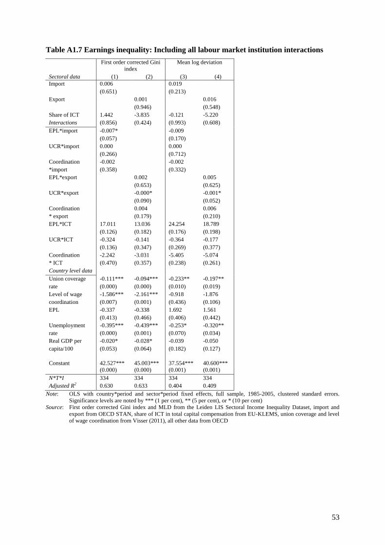
53

Table A1.7 Earnings inequality: Including all labour market institution interactions


index

Mean log deviation


Import 0.006 0.019

(0.651) (0.213)

Export 0.001 0.016

(0.946) (0.548)

Share of ICT 1.442 -3.835 -0.121 -5.220

Interactions (0.856) (0.424) (0.993) (0.608)

EPL*import -0.007* -0.009

(0.057) (0.170)

UCR*import 0.000 0.000

(0.266) (0.712)

Coordination -0.002 -0.002

*import (0.358) (0.332)

EPL*export 0.002 0.005

(0.653) (0.625)

UCR*export -0.000* -0.001*

(0.090) (0.052)

Coordination 0.004 0.006

* export (0.179) (0.210)

EPL*ICT 17.011 13.036 24.254 18.789

(0.126) (0.182) (0.176) (0.198)

UCR*ICT -0.324 -0.141 -0.364 -0.177

(0.136) (0.347) (0.269) (0.377)

Coordination -2.242 -3.031 -5.405 -5.074

* ICT (0.470) (0.357) (0.238) (0.261)

Country level data

Union coverage -0.111*** -0.094*** -0.233** -0.197**

rate (0.000) (0.000) (0.010) (0.019)

Level of wage -1.586*** -2.161*** -0.918 -1.876

coordination (0.007) (0.001) (0.436) (0.106)

EPL -0.337 -0.338 1.692 1.561

(0.413) (0.466) (0.406) (0.442)

Unemployment -0.395*** -0.439*** -0.253* -0.320**

rate (0.000) (0.001) (0.070) (0.034)

Real GDP per -0.020* -0.028* -0.039 -0.050

capita/100 (0.053) (0.064) (0.182) (0.127)

Constant

42.527***

45.003***

37.554***

40.600***

(0.000) (0.000) (0.001) (0.001)

N*T*I 334 334 334 334

Adjusted R2 0.630 0.633 0.404 0.409



Source: First order corrected Gini index and MLD from the Leiden LIS Sectoral Income Inequality Dataset, import and

export from OECD STAN, share of ICT in total capital compensation from EU-KLEMS, union coverage and level

of wage coordination from Visser (2011), all other data from OECD

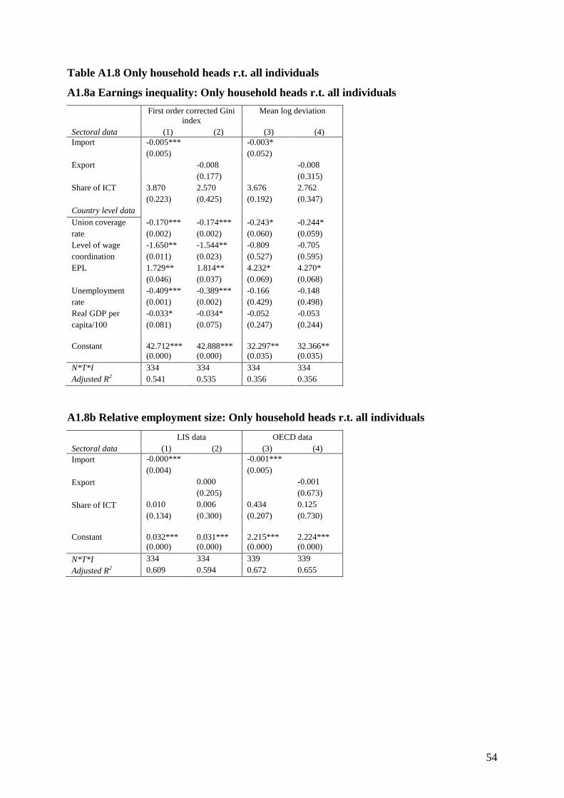
54

Table A1.8 Only household heads r.t. all individuals

A1.8a Earnings inequality: Only household heads r.t. all individuals


index

Mean log deviation


Import -0.005*** -0.003*

(0.005) (0.052)

Export -0.008 -0.008

(0.177) (0.315)

Share of ICT 3.870 2.570 3.676 2.762

(0.223) (0.425) (0.192) (0.347)

Country level data

Union coverage -0.170*** -0.174*** -0.243* -0.244*

rate (0.002) (0.002) (0.060) (0.059)

Level of wage -1.650** -1.544** -0.809 -0.705

coordination (0.011) (0.023) (0.527) (0.595)

EPL 1.729** 1.814** 4.232* 4.270*

(0.046) (0.037) (0.069) (0.068)

Unemployment -0.409*** -0.389*** -0.166 -0.148

rate (0.001) (0.002) (0.429) (0.498)

Real GDP per -0.033* -0.034* -0.052 -0.053

capita/100 (0.081) (0.075) (0.247) (0.244)

Constant

42.712***

42.888***

32.297**

32.366**

(0.000) (0.000) (0.035) (0.035)

N*T*I 334 334 334 334

Adjusted R2 0.541 0.535 0.356 0.356

A1.8b Relative employment size: Only household heads r.t. all individuals

LIS data OECD data


Import -0.000*** -0.001***

(0.004) (0.005)

Export 0.000 -0.001

(0.205) (0.673)

Share of ICT 0.010 0.006 0.434 0.125

(0.134) (0.300) (0.207) (0.730)

Constant

0.032***

0.031***

2.215***

2.224***

(0.000) (0.000) (0.000) (0.000)

N*T*I 334 334 339 339

Adjusted R2 0.609 0.594 0.672 0.655

55

A1.8c Relative median earnings: Only household heads r.t. all individuals



Import -0.000

(0.133)

Export 0.000

(0.822)


(0.729) (0.953)

Constant

0.944***

0.941***

(0.000) (0.000)

N*T*I 334 334

Adjusted R2 0.489 0.480







Table A1.9 Household r.t. individual earnings

A1.9a Earnings inequality: Household r.t. individual earnings


index

Mean log deviation


Import -0.003* -0.003

(0.067) (0.143)

Export -0.003 -0.002

(0.628) (0.764)

Share of ICT 5.341*** 4.633** 5.534** 4.829**

(0.006) (0.014) (0.037) (0.043)

Country level data

Union coverage -0.114*** -0.117*** -0.085** -0.089**

rate (0.000) (0.000) (0.021) (0.020)

Level of wage -1.820*** -1.782*** -2.382*** -2.354***

coordination (0.002) (0.001) (0.006) (0.005)

EPL 2.016** 2.077** 1.788 1.856

(0.047) (0.047) (0.131) (0.130)

Unemployment 0.031 0.038 0.099 0.105

rate (0.679) (0.559) (0.566) (0.524)

Real GDP per -0.030*** -0.031*** -0.030 -0.031

capita/100 (0.002) (0.002) (0.164) (0.157)

Constant

38.808***

38.941***

26.237***

26.387***

(0.000) (0.000) (0.004) (0.004)

N*T*I 334 334 334 334

Adjusted R2 0.615 0.610 0.574 0.570

56

A1.9b Relative employment size: Household r.t. individual earnings

LIS data OECD data


Import -0.002*** -0.001***

(0.005) (0.005)

Export 0.001 -0.001

(0.646) (0.673)

Share of ICT 0.791 0.422 0.434 0.125

(0.158) (0.429) (0.207) (0.730)

Constant

3.250***

3.214***

2.215***

2.224***

(0.000) (0.000) (0.000) (0.000)

N*T*I 334 334 339 339

Adjusted R2 0.551 0.535 0.672 0.655

A1.9c Relative median earnings: Household r.t. individual earnings



Import -0.000

(0.127)

Export 0.000

(0.975)

Share of ICT -0.080 -0.106

(0.487) (0.389)

Constant

0.985***

0.984***

(0.000) (0.000)

N*T*I 334 334

Adjusted R2 0.556 0.545







57

Appendix 2. Documentation Leiden LIS sectoral income inequality dataset

LEIDEN LIS SECTORAL INCOME INEQUALITY DATASET

Chen Wang, Stefan Thewissen, and Olaf van Vliet

Leiden University, Department of Economics

Version 1, June 2013

A2.1 Introduction

The Leiden LIS Sectoral Income Inequality Dataset contains information on multiple

indicators of earnings inequality and employment within 9 sectors and 12 subsectors for 12

developed countries and 49 LIS waves between 1969 and 2005. We provide additional

information of earnings and employment at the country level. This dataset draws upon data

from the Luxembourg Income Study (LIS) micro dataset, which is a time series of household

survey data containing information on earnings and employment, standardised across

countries. The Leiden LIS Sectoral Income Inequality Dataset allows researchers and public

policy analysts to compare sectoral earnings inequality and employment levels across

developed countries over the last three decades, based on a standardised classification of

sectors across countries and periods. The data can be linked to other sectoral databases, for

instance to the OECD Structural Analysis (STAN) database. The database extends the work

of Mahler, Jesuit, and Roscoe (1999) who calculate sectoral earnings inequality in 10

countries around the years 1985 and 1990. The full list of variable definitions can be found in

Appendix 3.

A2.2 Calculating sectoral earnings inequality and employment

Labour earnings and sample definition

We calculate annual earnings both at the household and individual level. We follow the

earnings and sample definitions of Mahler et al. (1999), that is, we only include income from

wages and salaries or self-employment. Income from other sources, such as interest and rent,

58

is excluded. Also excluded are public benefits and income taxes. For all calculations we apply

standard LIS top- and bottom coding conventions, with 1 per cent of (for household

inequality: equivalised) mean earnings as our bottom, and ten times the median (for

household inequality: non-equivalised) earnings as our top boundary.

We restrict our sample to ‘prime age workers’, people aged between 25 and 54 with

nonzero earnings following Mahler et al. (1999). This is the part of the population that is for

its income most dependent on earnings from labour. In addition, this group probably has the

strongest labour market attachment as their earnings are less affected by retirement and

schooling decisions (Atkinson et al., 1995; Mahler et al., 1999). Based on this sample, we

calculate the earnings inequality using household earnings (following Mahler et al., 1999) and

using individual earnings for multiple sample definitions.

For the calculations based on household earnings, we correct for differences in

household size using the square root equivalence scale. We apply household weights as

standard in LIS.35

We follow Mahler et al. (1999) by defining households as working in a

particular sector if the household head is working in this sector.36

Yet, a problem with using household earnings is that the members of a household

might work in different sectors, so that earnings are attributed to sectors in which they were

not necessarily made. Therefore, we also calculate inequality based on individual earnings.

We use the personal weights37

and we distinguish between three groups of individuals where

we again only include people aged between 25 and 54 with nonzero earnings:

1. Household heads;

2. Household heads and spouses;

3. All individuals.

Here, we attribute the individual earnings to the sector in which the specific individual is

working.38

We also show the absolute and relative number of households and individuals

classified in a sector, both weighted and unweighted, and their weighted absolute and median

earnings. The LIS weightings are used to transpose the sample indicators to the population

level. In this case, the population is the total number of households or individuals with the age

and earnings restriction.

35

HWEIGHT in LIS. 36

D16 in LIS. 37

PPOPWGT in LIS. 38

IND1_C in LIS.

59

Contrary to Mahler et al. (1999), we do not include sectoral information for disposable

income and the amount of redistribution, as taxes and transfers are set at the national level so

that these regulations do not differ between sectors.

Sectoral classification and country sample

We standardise the classification of sectors based on the International Standard of Industrial

Classification (ISIC) rev. 3.0 at the two digit level. The manufacturing and transport and

telecommunication sector are further broken down using the ISIC 3.0 three digit level, as can

be seen in Table A2.1.

Table A2.1 Sectoral definitions based on the ISIC 3.0 codes

No. Sector ISIC rev. 3.0 code

1 Agriculture, hunting, forestry and fishing C01T05

2 Mining and quarrying C10T14

3 Manufacturing C15T37

31 Food products, beverages and tobacco C15T16

32 Textiles, textile products, leather and footwear C17T19

33 Wood and products of wood and cork C20

34 Pulp, paper, paper products, printing and publishing C21T22

35 Chemical, rubber, plastics and fuel products C23T25

36 Other non-metallic mineral products C26

37 Basic metals and fabricated metal products C27T28

38 Machinery and equipment C29T33

39 Transport equipment C34T35

30 Manufacturing n.e.c. and recycling C36T37

4 Electricity, gas and water supply C40T41

5 Construction C45

6 Wholesale and retail trade – restaurants and hotels C50T55

7 Transport and telecommunications C60T64

71 Transport and storage C60T63

72 Post and telecommunications C64

8 Finance, insurance, real estate and business services C65T74

9 Community, social and personal services C75T99

In the LIS database multiple sectoral definitions are used across countries and waves, such as

ISIC 2.0, or NAICS for the US. To consistently classify industries, we recompute all

classification schemes to the ISIC 3.0 definitions. In general this did not require much

interpretation, although sometimes some sectors needed to be excluded (mainly when no

distinction was made between C34T35 Manufacturing of transport equipment and C36T37

Manufacturing n.e.c. and recycling). Seven classification dummies are included. The

classification scheme is included as a separate worksheet in the dataset.

60

As displayed in Table A2.2, for twelve developed countries data at the sectoral level are

available. Contrary to Mahler et al. (1999), we include Austria, Belgium, Czech Republic,

Ireland, Poland, and Spain. Yet, we leave out Australia, Canada, Italy, and the Netherlands for

which the data does not have enough detail to calculate inequality for a sufficient number of

sectors – only when certain sectors are combined data are available.

The three waves in italics in Table A2.2, the 2000 waves for Belgium, Ireland, and

Spain, are based on net earnings. The calculations for Germany in 1984 and 1989 are based

on West-Germany. For Ireland, three consecutive waves with only few observations, 1994-

1996, have been combined (with YEAR=1994-1996) where earnings information has been

recalculated to 1995 levels using information on inflation from the World Bank. Due to the

higher number of surveyed people, we recommend to use this combined observation for 1994-

1996 instead of the observations for the separate years. The inclusion of Spain, and to a lesser

extent Belgium, requires caution as the number of surveyed people is low, leading to possibly

inaccurate inequality estimations.

Table A2.2 Country and wave sample

Country Available waves

Austria 2004

Belgium 1995, 2000

Czech Republic 1996, 2004

Denmark 1987, 1992, 1995, 2000, 2004

Finland 1987, 1991, 1995, 2000, 2004

Germany 1984, 1989, 1994, 2000, 2004

Ireland 1994, 1995, 1996, 1994-1996, 2000, 2004

Poland 1986, 1992, 1995, 1999, 2004

Spain 1995, 2000

Sweden 1981, 1987, 1992, 2000, 2005

UK 1969, 1979, 1986, 1999, 2004

US 1979, 1986, 1991, 1994, 1997, 2000, 2004

For a number of variables information is missing for Austria, Belgium, Poland, Spain, the

waves with net earnings, the individual waves 1994-1996 for Ireland, Sweden 1981, UK 1969

and 1979, and the US 1979 and 1997. Thus, for these variables a total of 31 waves and 639

observations are available.

One possible application of this dataset is to use the data in panel data analysis. The

waves can be included in an unbalanced panel dataset of five year periods, for instance from

around 1985 to around 2005. This leads to the exclusion of the UK 1969 and 1979, Sweden

1981, and the US 1979 and 1997, and the three individual years 1994, 1995, and 1996 for

Ireland.

61

A2.3 Codebook and descriptives

Now we show definitions and descriptives of our main variables. In the summary statistics we

exclude the individual waves 1994, 1995, and 1996 for Ireland, but we do use the

combination 1994-1996. Thus, in the descriptives a maximum of 47 waves are included.

Country-level data based on household information

The dataset contains a number of indicators at the country level based on household

information. The first two columns in Table A2.3 show the sum of unweighted (SUM) and

weighted (SUMW) number of individuals within included households in the calculations at

the sectoral level in the respective wave. Next, GINIC shows the level of equivalised earnings

inequality as measured by the Gini indicator, pooled for all households part of our sectoral

sample. P50C gives us the weighted median household earnings. Its summary statistics are not

shown here as the indicator is expressed in national currency and current prices, making it not

internationally comparable.

Table A2.3 Country-level indicators based on household information

Variable name SUM SUMW GINIC

Mean 10,574 30,751,966 0.320

Standard dev. 11,136 53,294,823 0.049

Minimum 497 4,606 0.249

Maximum 39,944 176,450,466 0.455

No. waves 47 31 47

Thus, the average country-wave observation Gini is 0.320 based on household information.

Country-level data based on individual information

The following country-level indicators are included in the database constructed on the basis of

individual information. Table A2.4 shows the sum of the unweighted number of individuals

using the three groups of individuals (SUMALL for all individuals, SUMHS for household

heads and spouses, and SUMH for household heads only). Table A2.5 shows the same

information but then for the weighted frequencies.

62

Table A2.4 Unweighted individual frequencies at the country level

Variable name SUMALL SUMHS SUMH

Mean 18,013 16,495 10,353

Standard dev. 24,201 20,649 13,842

Minimum 743 511 363

Maximum 124,760 109,999 72,308

No. waves 44 44 44

Table A2.5 Weighted individual frequencies at the country level

Variable name SUMWALL SUMWHS SUMWH

Mean 20,338,100 18,132,199 11,958,302

Standard dev. 28,467,058 24,668,276 16,126,149

Minimum 1,140,132 943,437 569,594

Maximum 89,010,701 76,499,922 49,259,582

No. waves 31 31 31

Next, Table A2.6 summarises the level of inequality for the sample based on all individuals,

using a number of indicators. We report the Gini (GINIALLC), the mean log deviation

(GE0ALLC), the Theil index (GE1ALLC), and the Atkinson index with inequality aversion

parameter ε = 0.5 (AT05ALLC). The dataset also contains information on the median

individual earnings for the three sample definitions (P50ALLC, P50HSC, and P50HC), for

which summary statistics are not shown here as they are expressed in national currency and

current prices.

Table A2.6 Individual earnings inequality at the country level

Variable name GINIALLC GE0ALLC GE1ALLC AT05ALLC

Mean 0.322 0.234 0.193 0.098

Standard dev. 0.050 0.063 0.059 0.027

Minimum 0.257 0.152 0.125 0.066

Maximum 0.416 0.346 0.328 0.152

No. waves 31 31 31 31

Sectoral data based on household information

Now we move to sectoral data based on household information. In Table A2.7 we show

descriptives for the unweighted and weighted number of households per sector (FREQ and

WFREQ respectively). Next, RELFREQ shows the weighted relative employment size of a

sector, defined as the number of households classified in a sector divided by the total number

of households (WFREQ/SUMW * 100%). The relative employment size maps sectoral

employment shifts relative to the total labour market per country, sector, and over time. As an

example, the average sector contains 665 households.

63

Table A2.7 Frequencies and relative employment size based on household information

Variable name FREQ WFREQ RELFREQ

Mean 665 1,924,483 6.413

Standard dev. 1,354 5,608,224 7.562

Minimum 2 22 0.139

Maximum 13,115 50,300,000 40.373

No. observ. 960 639 639

Next, Table A2.8 summarises descriptives for sectoral earnings inequality for multiple

indicators based on equivalised household information. We report the Gini (GINI), the

P90/P10 ratio (P90P10), the mean log deviation (GE0), the Theil index (GE1), and the

Atkinson index with inequality aversion parameter ε = 0.5 (AT05). The Gini coefficient is to a

certain extent sensitive to the sample size for which the Gini is calculated. For the Gini

bootstrapped standard errors with 250 repeats are calculated (BSSE250) to provide a

confidence interval of the level of inequality.

Deltas (2003) shows this for different cumulative distributions, using Monte Carlo

simulations. When the sample size becomes lower, the Gini starts to underestimate the ‘true’

inequality level. Deltas calculates that by multiplying the Gini by N / (N – 1), which he calls

the first order correction, the underestimation bias is significantly reduced. As for some

industries, in particular mining and wood manufacturing, the number of people interviewed is

often low, we include his first order procedure by calculating GINIFOC as the GINI * FREQ /

(FREQ – 1). We use the unweighted frequencies here as the bias arises from the number of

people interviewed (the sample).

Last, we show the relative median wage (BETWEEN), a measure of inequality

between rather than within industries, calculated as the sectoral median wage divided by its

counterpart at the national level (P50/P50C). Again, summary statistics for the P50 are not

shown here as the indicator is expressed in national currency and current prices, so that it is

not internationally comparable.

Table A2.8 Earnings inequality based on household information

Variable name GINI GINIFO

C BSSE250 P90P10 GE0 GE1 AT05

BETWEE

N

Mean 0.289 0.294 0.022 4.918 0.175 0.153 0.076 1.087

Standard dev. 0.062 0.069 0.019 12.813 0.099 0.099 0.036 0.192

Minimum 0.095 0.119 0.002 1.813 0.027 0.027 0.013 0.091

Maximum 0.608 1.216 0.304 360.243 1.514 0.858 0.457 1.980

No. observ. 960 960 960 960 960 960 960 960

64

Sectoral data based on individual information

The first three columns of Table A2.9 summarise the unweighted number of persons

classified in a sector for the three groups of individuals. Columns 4-6 provide the same

information for the weighted number of persons.

Table A2.9 Frequencies based on individual information

Variable name FREQALL FREQHS FREQH WFREQALL WFREQHS WFREQH

Mean 1,078 988 637 1,245,758 1,113,643 755,462

Standard dev. 3,031 2,738 1,669 3,321,328 2,917,900 1,832,553

Minimum 4 2 1 1201 1,201 974

Maximum 42,064 37,096 24,418 28,600,000 25,300,000 15,100,000

No. observ. 900 900 900 639 639 639

Table A2.10 describes the weighted relative employment size of a sector, defined as the

number of individuals classified in a sector divided by the total number of individuals for the

three groups of individuals.

Table A2.10 Relative employment size based on individual information

Variable name RELFREQALL RELFREQHS RELFREQH

Mean 0.062 0.062 0.064

Standard dev. 0.084 0.085 0.078

Minimum 0.001 0.001 0.001

Maximum 0.438 0.440 0.386

No. observ. 639 639 639

Next, we show in Table A2.11 the Gini for the three groups of individuals, both the ‘normal’

one and the first-order corrected version, which decreases bias due to small sample size.

Table A2.11 Gini based on individual information

Variable name GINIALL GINIHS GINIH GINIALLFOC GINIHSFOC GINIHFOC

Mean 0.281 0.280 0.263 0.282 0.284 0.268

Standard dev. 0.075 0.076 0.075 0.076 0.078 0.078

Minimum 0.078 0.078 0.078 0.083 0.083 0.082

Maximum 0.597 0.601 0.594 0.654 0.845 0.750

No. observ. 900 900 899 900 900 899

Table A2.12 provides information on the mean log deviation (MLD) or GE(0) and the

weighted relative median wage for the three groups of individuals. These are again calculated

by dividing the sectoral median wage by its counterpart at the country level. Again, summary

statistics for the sectoral median wage themselves are not shown here because they are

65

expressed in national currency and current prices and therefore not internationally

comparable.

Table A2.12 MLD and relative median wage based on individual earnings

Variable name GE0ALL GE0HS GE0H BETWEENALL BETWEENHS BETWEENH

Mean 0.185 0.184 0.165 1.050 1.048 1.017

Standard dev. 0.112 0.115 0.114 0.194 0.195 0.185

Minimum 0.010 0.010 0.010 0.159 0.151 0.145

Maximum 1.099 1.143 1.130 1.925 1.844 2.767

No. observ. 638 638 638 639 639 639

A2.4 Comparison to Mahler et al. (1999)

Comparing to Mahler et al. (1999), we extend the dataset of sectoral earnings inequality in

three ways as can be seen in Table A2.13. Firstly, we calculate earnings inequality for 12

countries and between 1969 and 2005, while Mahler et al. (1999) provide data for 10

countries and between 1984 and 1992. Secondly, we include more inequality measures.

Mahler et al. only calculate the P90/P10 whilst we also include the Gini, the Atkinson index

(ε =0.5), the mean log deviation (GE(0)), and the Theil index (GE(1)) for household earnings.

Next to calculations based on household information, we calculate the GE(0) and Gini using

individual information, which allows us to more carefully attribute earnings to sectors. In

addition, we follow the first order correction to reduce the underestimation bias by low

sample size.

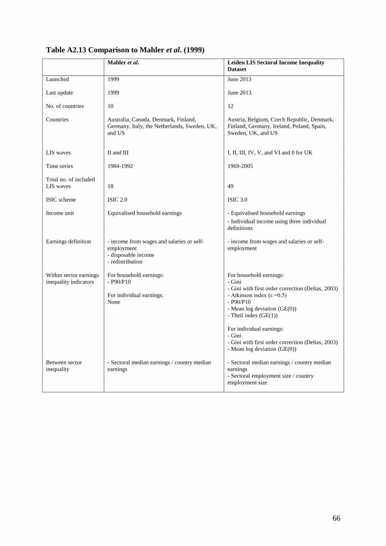
66

Table A2.13 Comparison to Mahler et al. (1999)

Mahler et al. Leiden LIS Sectoral Income Inequality

Dataset

Launched 1999 June 2013

Last update 1999 June 2013

No. of countries 10 12

Countries Australia, Canada, Denmark, Finland,

Germany, Italy, the Netherlands, Sweden, UK,

and US

Austria, Belgium, Czech Republic, Denmark,

Finland, Germany, Ireland, Poland, Spain,

Sweden, UK, and US

LIS waves II and III I, II, III, IV, V, and VI and 0 for UK

Time series 1984-1992 1969-2005

Total no. of included

LIS waves

18

49

ISIC scheme ISIC 2.0 ISIC 3.0

Income unit Equivalised household earnings - Equivalised household earnings

- Individual income using three individual

definitions

Earnings definition - income from wages and salaries or self-

employment

- disposable income

- redistribution

- income from wages and salaries or self-

employment

Within sector earnings

inequality indicators

For household earnings:

- P90/P10

For individual earnings:

None

For household earnings:

- Gini

- Gini with first order correction (Deltas, 2003)

- Atkinson index (ε =0.5)

- P90/P10

- Mean log deviation (GE(0))

- Theil index (GE(1))

For individual earnings:

- Gini

- Gini with first order correction (Deltas, 2003)

- Mean log deviation (GE(0))

Between sector

inequality

- Sectoral median earnings / country median

earnings

- Sectoral median earnings / country median

earnings

- Sectoral employment size / country

employment size

67

Appendix 3. Full variable list of the Leiden LIS Sectoral Income Inequality Dataset

version 1

Variable name Definition

Identifiers

COU Country abbreviation

CNTRY Country code

YEAR LIS survey year

PERIOD

Period number {1, …6} (for panel data analysis, with six periods of each around five years between

1980-2005)

INDUS Sectoral code based on ISIC rev. 3.0

CLASSIFICATION Full sectoral name based on ISIC rev. 3.0

Industry classification scheme

ISIC 3

Dummy for ISIC 3.0 (ISIC 3=1 if the LIS micro data (variable D16) of that wave is classified based

on ISIC 3.0)

ISIC 2

Dummy for ISIC 2.0 (ISIC 2=1 if the LIS micro data (variable D16) of that wave is classified based

on ISIC 2.0)

SIC Dummy for SIC (SIC=1 if the LIS micro data (variable D16) of that wave is classified based on SIC)

OLD NAICS

Dummy for old NAICS classification (OLD NAICS=1 if the LIS micro data (variable D16) of that

wave is classified based on an older version of NAICS classification)

NEW NAICS

Dummy for new NAICS classification (NEW NAICS=1 if the LIS micro data (variable D16) of that

wave is classified based on the new version of NAICS classification)

Other

Dummy for other classification schemes (OTHER=1 if the LIS micro data (variable D16) of that

wave is classified based on none of the aforementioned classification schemes

NET EARN Dummy indicating waves for which net earnings are used

WGD Dummy for West Germany (WGD=1 for Germany 1989, 1994)

Country level data based on household information

SUM

Total number of individuals within households with household head aged 25-54 with nonzero

household earnings classified in a sector

SUMW

Total weighted number of individuals within households with household head aged 25-54 with

nonzero household earnings classified in a sector

GINIC

Gini for households with household head aged 25-54 with nonzero household earnings classified in a

sector

P50C

Weighted median household earnings with household head aged 25-54 with nonzero household

earnings classified in a sector in national currency, current prices

Country level data based on individual information

SUMALL Total number of all individuals aged 25-54 with nonzero earnings classified in a sector

SUMHS

Total number of household heads and spouses aged 25-54 with nonzero earnings classified in a

sector

SUMH Total number of household heads aged 25-54 with nonzero earnings classified in a sector

SUMWALL Total weighted number of individuals aged 25-54 with nonzero earnings classified in a sector

SUMWHS

Total weighted number of household heads and spouses aged 25-54 with nonzero earnings classified

in a sector

SUMWH Total weighted number of household heads aged 25-54 with nonzero earnings classified in a sector

GINIALLC Gini for all individuals aged 25-54 with nonzero earnings classified in a sector

GE0ALLC Mean log deviation for all individuals aged 25-54 with nonzero earnings classified in a sector

GE1ALLC Theil index for all individuals aged 25-54 with nonzero earnings classified in a sector

AT05ALLC Atkinson's index (0.5) for all individuals aged 25-54 with nonzero earnings classified in a sector

P50ALLC

Weighted median earnings for all individuals aged 25-54 with nonzero earnings classified in a sector

in national currency, current prices

P50HSC

Weighted median earnings for household heads and spouses aged 25-54 with nonzero earnings

classified in a sector in national currency, current prices

P50HC Weighted median earnings for household heads aged 25-54 with nonzero earnings classified in a

68

sector in national currency, current prices

Sectoral data based on household information

FREQ Number of households with household head aged 25-54 with nonzero earnings

WFREQ Weighted number of households with household head aged 25-54 with nonzero earnings

RELFREQ Weighted relative sectoral employment size: WFREQ / SUMW * 100%

GINI

Sectoral Gini (without first order correction) of households with household head 25-54 with nonzero

household earnings

GINIFOC

Sectoral Gini first order corrected based on Deltas (2003): FREQ / (FREQ – 1) * GINI, of

households with household head 25-54 with nonzero household earnings

BSSE250 Bootstrapped standard errors of the sectoral Gini (without first order correction) with 250 repeats

P90P10 Sectoral P90/P10 ratio of households with household head 25-54 with nonzero household earnings

GE0

Sectoral mean log deviation of households with household head 25-54 with nonzero household

earnings

GE1 Sectoral Theil index of households with household head 25-54 with nonzero household earnings

AT05

Sectoral Atkinson index with parameter ε = 0.5 of households with household head 25-54 with

nonzero household earnings

P50

Weighted sectoral median earnings with household head aged 25-54 with nonzero household

earnings, national currency, current prices

BETWEEN Weighted relative sectoral median wage or inequality between sectors: P50 / P50C

Sectoral data based on individual information

FREQALL Number of all individuals aged 25-54 with nonzero earnings

FREQHS Number of household heads and spouses aged 25-54 with nonzero earnings

FREQH Number of household heads aged 25-54 with nonzero earnings

WFREQALL Weighted number of all individuals aged 25-54 with nonzero earnings

WFREQHS Weighted number of household heads and spouses aged 25-54 with nonzero earnings

WFREQH Weighted number of household heads aged 25-54 with nonzero earnings

RELFREQALL Weighted relative sectoral employment size, all individuals: WFREQALL / SUMWALL * 100%

RELFREQHS

Weighted relative sectoral employment size, household heads and spouses: WFREQHS / SUMWHS

* 100%

RELFREQH Weighted relative sectoral employment size, household heads: WFREQH / SUMWH * 100%

GINIALL Sectoral Gini (without first order correction) forall individuals aged 25-54 with nonzero earnings

GINIHS

Sectoral Gini (without first order correction) for household heads and spouses aged 25-54 with

nonzero earnings

GINIH Sectoral Gini (without first order correction) for household heads aged 25-54 with nonzero earnings

GINIALLFOC

Sectoral Gini first order corrected based on Deltas (2003): FREQALL / (FREQALL – 1) *

GINIALL, all individuals aged 25-54 with nonzero earnings

GINIHSFOC

Sectoral Gini first order corrected based on Deltas (2003): FREQHS / (FREQHS – 1) * GINIHS,

household heads and spouses aged 25-54 with nonzero earnings

GINIHFOC

Sectoral Gini first order corrected based on Deltas (2003): FREQH / (FREQH – 1) * GINIH,

household heads aged 25-54 with nonzero earnings

GE0ALL Sectoral mean log deviation for all individuals aged 25-54 with nonzero earnings

GE0HS Sectoral mean log deviation for household heads and spouses aged 25-54 with nonzero earnings

GE0H Sectoral mean log deviation for household heads aged 25-54 with nonzero earnings

P50ALL

Weighted median individual earnings for all individuals aged 25-54 with nonzero earnings, national

currency, current prices

P50HS

Weighted median individual earnings for household heads and spouses aged 25-54 with nonzero

earnings, national currency, current prices

P50H

Weighted median individual earnings for household heads aged 25-54 with nonzero earnings,

national currency, current prices

BETWEENALL

Weighted relative sectoral median wage or inequality between sectors, all individuals: P50ALL /

P50ALLC

BETWEENHS

Weighted relative sectoral median wage or inequality between sectors, household heads and spouses:

P50HS / P50HSC

BETWEENH

Weighted relative sectoral median wage or inequality between sectors, household heads: P50H /

P50HC

lis working paper series · we thank koen caminada, ... 2012 nig conference in leuven, and the 2013...

Documents