lecture 3 notes espm 228 micromet flux measurements eddy...

ESPM 228, Advanced Topics in Biometeorology and Micrometeorology

1

Lecture 3 Micromet Flux Measurements, Eddy Covariance, Part 1 Instructor: Dennis Baldocchi Professor of Biometeorology Ecosystems Science Division Department of Environmental Science, Policy and Management 345 Hilgard [email protected] 642-2874 January 30, 2014 Outline

a. Eddy Covariance method. i. Theoretical Basis ii. Density corrections iii. Storage and non-steady state conditions

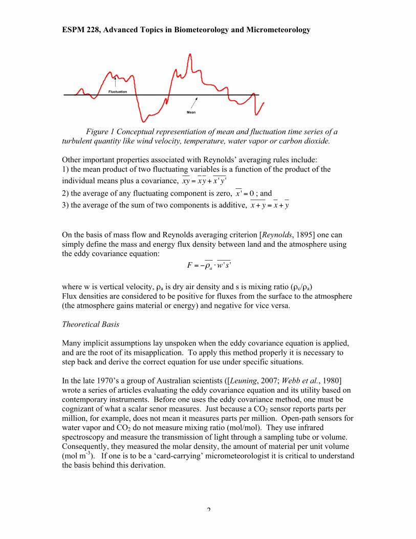
Eddy Covariance Method The eddy covariance method is a micrometeorologically-based method of measuring turbulent fluxes in the internal boundary layer of the atmosphere. The method is generally applied above the atmosphere/vegetation interface, [Aubinet et al., 2000; D.D. Baldocchi, 2003; D. D. Baldocchi et al., 1988; Pattey et al., 2006], but a growing number of studies are showing it can be applied within vegetation, too. The technique has many advantages over other methods used by biogeoscientists. It is a direct measure of the flux density, it is in situ, it introduces no artifact on the system it is measuring, it is quasi-continuous and represents a large upwind extent. Reynolds’ Rules of Averaging are used to provide a statistical representation of turbulent wind, its non-Gaussian attributes and turbulent fluxes [Reynolds, 1895]. The motion of a turbulent fluid, like air, can be defined at any instant in time as being equal to the sum of its mean state ( x ) and is fluctuation from the mean ( x ' ); the overbar represents time averaging and the prime represents a fluctuation from the mean (Figure 1).


2

Figure 1 Conceptual representiation of mean and fluctuation time series of a

turbulent quantity like wind velocity, temperature, water vapor or carbon dioxide. Other important properties associated with Reynolds’ averaging rules include: 1) the mean product of two fluctuating variables is a function of the product of the individual means plus a covariance, xy = xy+ x ' y ' 2) the average of any fluctuating component is zero, x ' = 0 ; and 3) the average of the sum of two components is additive, x + y = x + y On the basis of mass flow and Reynolds averaging criterion [Reynolds, 1895] one can simply define the mass and energy flux density between land and the atmosphere using the eddy covariance equation:

F = −ρa ⋅w 's ' where w is vertical velocity, ρa is dry air density and s is mixing ratio (ρc/ρa) Flux densities are considered to be positive for fluxes from the surface to the atmosphere (the atmosphere gains material or energy) and negative for vice versa. Theoretical Basis Many implicit assumptions lay unspoken when the eddy covariance equation is applied, and are the root of its misapplication. To apply this method properly it is necessary to step back and derive the correct equation for use under specific situations. In the late 1970’s a group of Australian scientists ([Leuning, 2007; Webb et al., 1980] wrote a series of articles evaluating the eddy covariance equation and its utility based on contemporary instruments. Before one uses the eddy covariance method, one must be cognizant of what a scalar senor measures. Just because a CO2 sensor reports parts per million, for example, does not mean it measures parts per million. Open-path sensors for water vapor and CO2 do not measure mixing ratio (mol/mol). They use infrared spectroscopy and measure the transmission of light through a sampling tube or volume. Consequently, they measured the molar density, the amount of material per unit volume (mol m-3). If one is to be a ‘card-carrying’ micrometeorologist it is critical to understand the basis behind this derivation.

Mean

Fluctuation


3

From first principles, the flux of material across a horizontal plane is a function of the velocity of the air, the density of the air and the relative amount of scalar material in the parcel of air. To produce a conservative expression that defines a turbulent flux density, we can express the flux covariance derivation in terms of mixing ratio, the relative value

for the mean scalar density ( s = (ρcρa) ) or the ratio of partial pressures (S = pc

pa= (maρcmcρa

) ).

Combining w, ρa and s and averaging the product allows us to express the mean scalar flux density:

F = ρaws = ρamc

ma

wS

Applying Reynolds decomposition theory to the product of the vertical velocity, w, and the normalized scalar density, s, yields:

ρaws = (w+w ')(s+ s ')(ρa + ρa ') =

wρc = (w+w ')(ρc + ρc ')

Lets examine the expansion of ρaws first. The resulting multiplication produces 8 terms. They are: ρa ⋅w ⋅ s ' , ρa ⋅ s ⋅w ' , ρa ⋅w ⋅ s , ρa ⋅w 's ' s ⋅w ⋅ρa ' , w '⋅ s 'ρa ' , w ⋅ s '⋅ρa ' , s ⋅w '⋅ρa '

From Reynolds rules of averaging we know that averages of fluctuations equal zero, so the following terms equal zero: ρa ⋅w ⋅ s ' , ρa ⋅ s ⋅w ' , s ⋅w ⋅ρa ' . The covariance between w’ and ρa’ ( s ⋅w '⋅ρa ' ) can be evaluated by studying the flux of dry air. By definition the flux density of dry air is zero (in contrast the flux density of moist air equals the evaporation flux density).

wρa = w 'ρa '+wρa = 0 This equation leads to w 'ρa ' = −wρa and, with appropriate substitution, causes ρa ⋅w ⋅ s

and s ⋅w '⋅ρa ' to cancel one another. At this stage we are left with three terms: ρa ⋅w 's ' ,

w ⋅ s '⋅ρa ' and w '⋅ s 'ρa ' . Further inspection will reduce this trio to one term.


4

Going back to our definition of the flux of dry air we can arrive at an equation for the mean vertical velocity, w = −w 'ρa ' / ρa . Substitution of w into w ⋅ s '⋅ρa ' yields a fourth

order moment, −w 'ρa '⋅ s '⋅ρa 'ρa

. In comparison to ρa ⋅w 's ' , the remaining third (

w '⋅ s 'ρa ' ) and fourth (w ⋅ s 'ρa ' ) order terms can be neglected.

At this stage we now have an asymmetric equality between an eddy covariance: F = ρaws ≈ ρa ⋅w 's ' If we expand F = wρc we arrive at an expression defined as:

F = wρc = w 'ρc '+wρc The principle lesson to learn is that the following identify defined the Flux

Covariance: F = ρaws ≈ ρa ⋅w 's ' = wρc = w 'ρc '+wρc

The covariance between w and s equals the sum of the covariance between w and ρc and the product of the mean vertical velocity and scalar density, a mean drift term. The magnitude of this vertical velocity very small (1 to 2 mm s-1) and is below the resolution of most anemometry. Nevertheless, since it is multiplied times a scalar mole density, whose magnitude may be large (e.g. 580 mg m-3 for CO2), its product can result in a significant flux density.

As an aside we can arrive at the above equation by defining s fluctuations using rules for simple differential operators:

δs(ρc,ρa ) =∂s∂ρc

δρc +∂s∂ρa

δρa

s ' = (ρcρa)' = ρc

'

ρa−ρcρa2 ρa

'

Substituting into the w 's ' yields:

w 's ' = w 'ρc'

ρa−ρcρa2w 'ρa

' =w 'ρc

'

ρa+ρcwρa

And:


5

F = ρaw 's ' = wρc = w 'ρc '+wρc As was stressed above, most eddy covariance systems do not measure ρaw 's ' . Instead

they measure wρc , so we need to assess the term wρc . To do so, let’s evaluate

w = −w 'ρa ' / ρa and insert it into the above equation. For dry air, we can apply Boussinesq approximation yields:

ρa'

ρa= −

T 'T

and an equation for F that is a function of the vertical velocity-temperature covariance

F = w 'ρc '+ρcTw 'T '

If this addition of a heat flux sounds strange to evaluating a flux of a mole density, I like to step back and consider a controlled volume. Its mole density will change if we change the number of molecules we pack into the volume, or if the volume expands or contracts. If we consider an imaginary volume under a imaginary line across the atmosphere, flux will occur if the volume expands and crosses that line.

Figure 2 Cartoon showing mass transfer due to volumetric expansion of an air

parcel due to T fluctuations

In the field, the air is not dry. Instead we have to consider the case of moist air and fluctuations of temperature and moisture. When the air is moist, we work with the law of partial pressures and the gas law:


6

p = pa + pv

p = RmρT

ρama

+ρvmv

=pRT

Expansion analysis produces

ρa 'ma

+ρv 'mv

= −pRT

T 'T+...

Solving for air density fluctuations produce

ρa ' = −ma

mv

ρv' − ρa (1+

ρvma

ρamv

)T 'T

From which we can derive a new equation for the mean vertical velocity

w = −w 'ρa ' / ρa =ma

mv

w 'ρv'

ρa+ (1+ ρvma

ρamv

)w 'T 'T

The magnitude of w is on the order of 1 to 2 mm/s. In contrast, most state of art anemometers measure around 1 to cm/s. Though this magnitude is very small and is difficult to feel or detect, it can move a significant amount of mass. The background CO2 concentration of about 365 ppp yields a mass density equal to about 638 mg m-3. When multiplied by 1 mm/s, it can produce a flux density of 0.638 mg m-2 s-1 or 14.5 µmol m-2 s-1. In other words, a supposively small bias velocity can move a substantial amount of CO2. So far we have neglected Pressure fluctuations. Massman argues that corrections imposed by P fluctuations can be significant at high altitudes under high wind speeds. Near sea level pressure fluctuations are only a few pascals or 0.01% of atmospheric pressure [Gu et al., 2012; Massman and Lee, 2002] (< 10 Pa/100000Pa). Substitution into the flux equation produces the final Webb-Pearman-Leuning algorithm for computing flux densities with sensors that measure molar or mass volume:

Fc = w 'ρc '+ma

mv

ρcρaw 'ρv

' + (1+ ρvma

ρamv

) ρcTw 'T '


7

This final equation is the Webb-Pearman-Leuning equation we use to correction open-path measurements of CO2 flux densities. It is a function of the evaporation and sensible heat flux densities, as well as the amount of scalar material in the atmosphere and air temperature. An engineering version of this equation is: Fc = w 'ρc '+ 7.386 ⋅10

−3λE + 0.0383H (µmol m-2 s-1) Depending on the magnitudes of H and LE, the correction can vary widely. Hence, accurate measurements of H and LE are needed to derive accurate values of Fc.

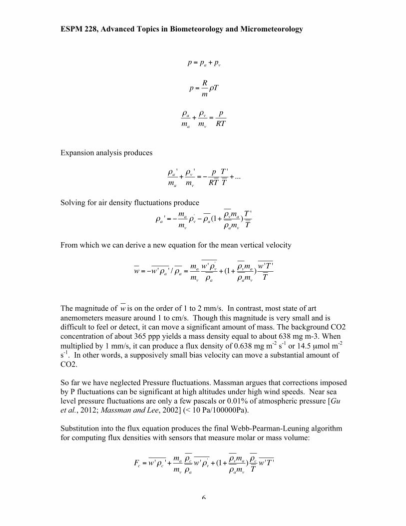
Table 1 Estimation of terms in the WPL theory

Fc w c' 'ρ H λE Error 16.49 5 300 0 0.696786 11.49 0 300 0 1

6.49 -5 300 0 1.770416 1.49 -10 300 0 7.711409

-8.51 -20 300 0 -1.35018 -18.51 -30 300 0 -0.62075

11.0458 5 100 300 0.547339

6.0458 0 100 300 1 1.0458 -5 100 300 5.781029

-3.9542 -10 100 300 -1.52896 -13.9542 -20 100 300 -0.43326 -23.9542 -30 100 300 -0.25239

6.778 5 -50 500 0.262319 1.778 0 -50 500 1

-3.222 -5 -50 500 -0.55183 -8.222 -10 -50 500 -0.21625

-18.222 -20 -50 500 -0.09757 -28.222 -30 -50 500 -0.063


8

WBW 1996

Fc wpl (µmol m-2 s-1)

-35 -30 -25 -20 -15 -10 -5 0 5 10

w'c

' (µ

mol

m-2

s-1

)

-35

-30

-25

-20

-15

-10

-5

0

5

10

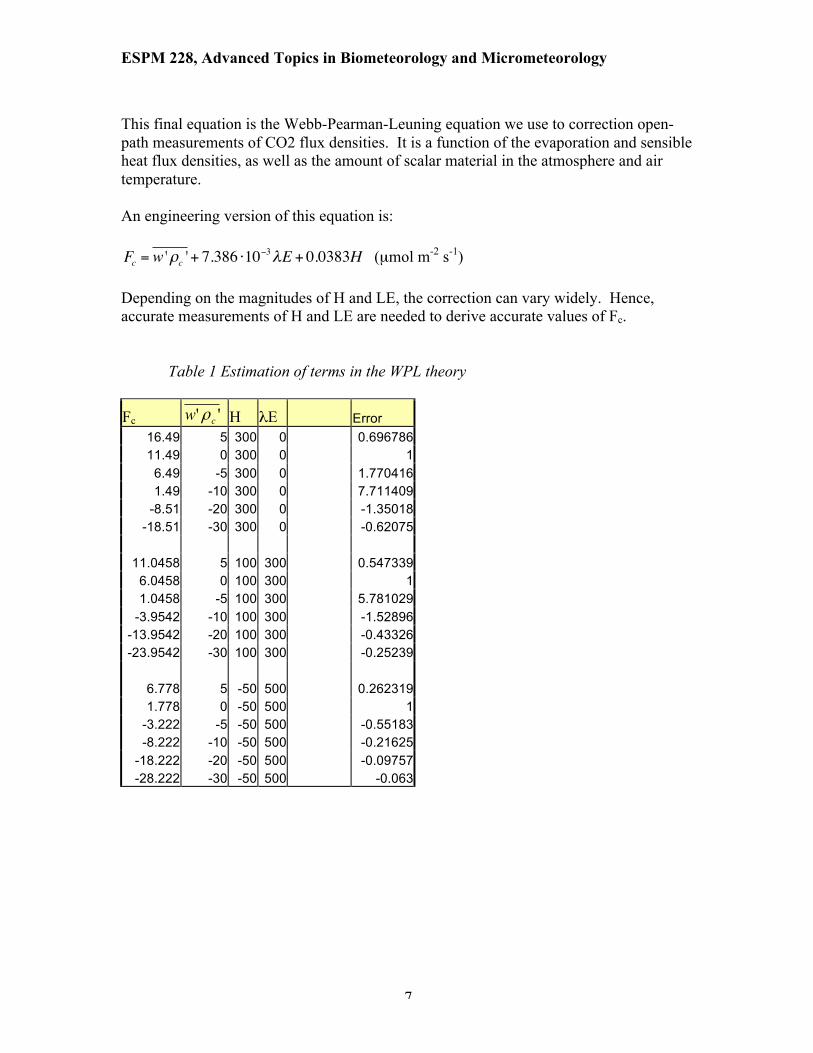
Figure 3 Comparison of direct eddy covariance measurement of CO2 and that

corrected for density fluctuations. Note that the differences can exceed 40% under certain conditions. This case was for a humid and temperate deciduous forest where LE is generally greater than H. The theory described above has been verified by field measurements. Leuning and colleagues performed a classic experimental test of the Webb et al density correction [Leuning et al., 1982]. They measured CO2 exchange over a bare field. Bare fields do not photosynthesize and only respire. The uncorrected CO2 flux density was directed downward, as the dry field was generated a large amount of sensible heat. When the density corrections were applied to the measurements, their data then yielded upward directed fluxes. And recently Ham and Heilman [Ham and Heilman, 2003] tested the WPL theory over a parking lot at KSU. We observed the same similar results in our own work over senescent grassland, which experiences sensible heat flux densities exceeding 300 W m-2. Uncorrected eddy fluxes suggested photosynthesis by the dead grass! The point to be made is that over fields that generate substantial heat and support small fluxes of CO2, ignoring the density corrections can not only yield erroneous results but infer a flux that is in the wrong direction!! Only with WPL corrections were we able to detect respiration by the system.


9

Grassland

w'ρc' (µmol m-2 s-1)

-15 -10 -5 0 5

F wpl (µ

mol

m-2

s-1

)

-4

-2

0

2

4

6

8

10

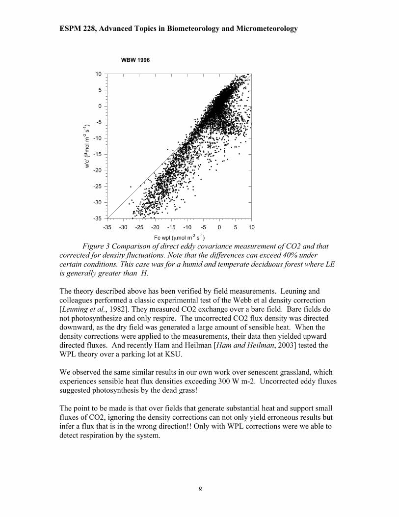
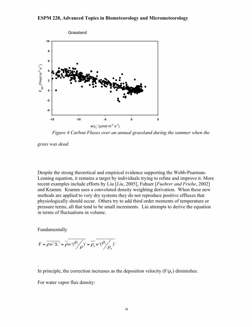
Figure 4 Carbon Fluxes over an annual grassland during the summer when the

grass was dead.

Despite the strong theoretical and empirical evidence supporting the Webb-Pearman-Leuning equation, it remains a target by individuals trying to refute and improve it. More recent examples include efforts by Liu [Liu, 2005], Fuhuer [Fuehrer and Friehe, 2002] and Kramm. Kramm uses a convoluted density weighting derivation. When these new methods are applied to very dry systems they do not reproduce positive effluxes that physiologically should occur. Others try to add third order moments of temperature or pressure terms, all that tend to be small increments. Liu attempts to derive the equation in terms of fluctuations in volume. Fundamentally

F = ρw 'S* ' = ρw '(ρcρ )' = ρaw '(

ρcρa)'

. In principle, the correction increases as the deposition velocity (F/ρc) diminishes. For water vapor flux density:


10

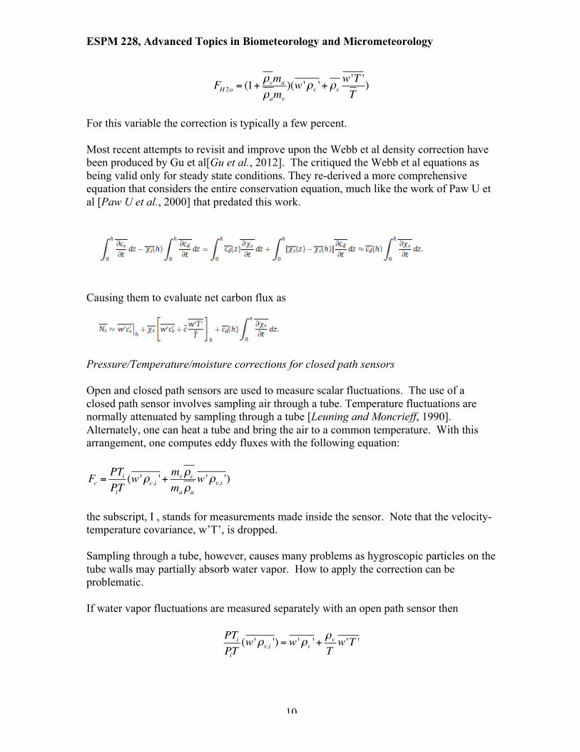
FH 2o = (1+ρvma

ρamv

)(w 'ρv '+ ρvw 'T 'T)

For this variable the correction is typically a few percent. Most recent attempts to revisit and improve upon the Webb et al density correction have been produced by Gu et al[Gu et al., 2012]. The critiqued the Webb et al equations as being valid only for steady state conditions. They re-derived a more comprehensive equation that considers the entire conservation equation, much like the work of Paw U et al [Paw U et al., 2000] that predated this work.

Causing them to evaluate net carbon flux as

Pressure/Temperature/moisture corrections for closed path sensors Open and closed path sensors are used to measure scalar fluctuations. The use of a closed path sensor involves sampling air through a tube. Temperature fluctuations are normally attenuated by sampling through a tube [Leuning and Moncrieff, 1990]. Alternately, one can heat a tube and bring the air to a common temperature. With this arrangement, one computes eddy fluxes with the following equation:

Fc =PTiPiT

(w 'ρc,i '+mvρcmaρa

w 'ρv,i ')

the subscript, I , stands for measurements made inside the sensor. Note that the velocity-temperature covariance, w’T’, is dropped. Sampling through a tube, however, causes many problems as hygroscopic particles on the tube walls may partially absorb water vapor. How to apply the correction can be problematic. If water vapor fluctuations are measured separately with an open path sensor then

PTiPiT

(w 'ρv,i ') = w 'ρv '+ρvTw 'T '


11

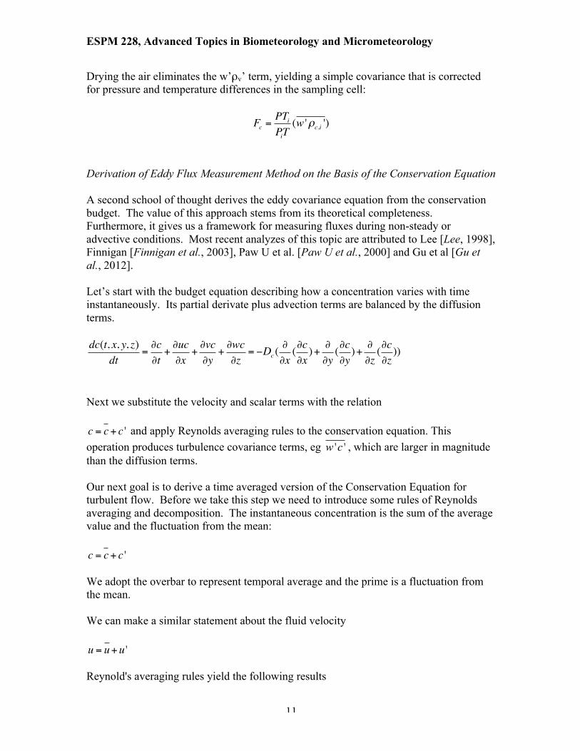
Drying the air eliminates the w’ρv’ term, yielding a simple covariance that is corrected for pressure and temperature differences in the sampling cell:

Fc =PTiPiT

(w 'ρc,i ')

Derivation of Eddy Flux Measurement Method on the Basis of the Conservation Equation A second school of thought derives the eddy covariance equation from the conservation budget. The value of this approach stems from its theoretical completeness. Furthermore, it gives us a framework for measuring fluxes during non-steady or advective conditions. Most recent analyzes of this topic are attributed to Lee [Lee, 1998], Finnigan [Finnigan et al., 2003], Paw U et al. [Paw U et al., 2000] and Gu et al [Gu et al., 2012]. Let’s start with the budget equation describing how a concentration varies with time instantaneously. Its partial derivate plus advection terms are balanced by the diffusion terms. dc(t, x, y, z)

dt=∂c∂t+∂uc∂x

+∂vc∂y

+∂wc∂z

= −Dc (∂∂x(∂c∂x)+ ∂∂y(∂c∂y)+ ∂∂z(∂c∂z))

Next we substitute the velocity and scalar terms with the relation c = c+ c ' and apply Reynolds averaging rules to the conservation equation. This operation produces turbulence covariance terms, eg w 'c ' , which are larger in magnitude than the diffusion terms. Our next goal is to derive a time averaged version of the Conservation Equation for turbulent flow. Before we take this step we need to introduce some rules of Reynolds averaging and decomposition. The instantaneous concentration is the sum of the average value and the fluctuation from the mean: c = c+ c ' We adopt the overbar to represent temporal average and the prime is a fluctuation from the mean. We can make a similar statement about the fluid velocity u = u+u ' Reynold's averaging rules yield the following results


12

1. The average of the average is the average: c = c 2. The average of the product of an average and an instantaneous value equals the product of the averages. ca = ca 3. The average of two sums equals the sum of the averages: a+ c = a+ c 4. The average of fluctuations is zero: c ' = 0 (c+ c ') = c c'c = 0 5. The average of the product of two variables equals the product of the averages plus a mean covariance term: cc = (c+ c ') ⋅ (c+ c ') = cc+ c 'c ' ca = (c+ c ') ⋅ (a+ a ') = ca+ c 'a ' 6. The average of the slopes equals the slope of the averages dcdt=dcdt

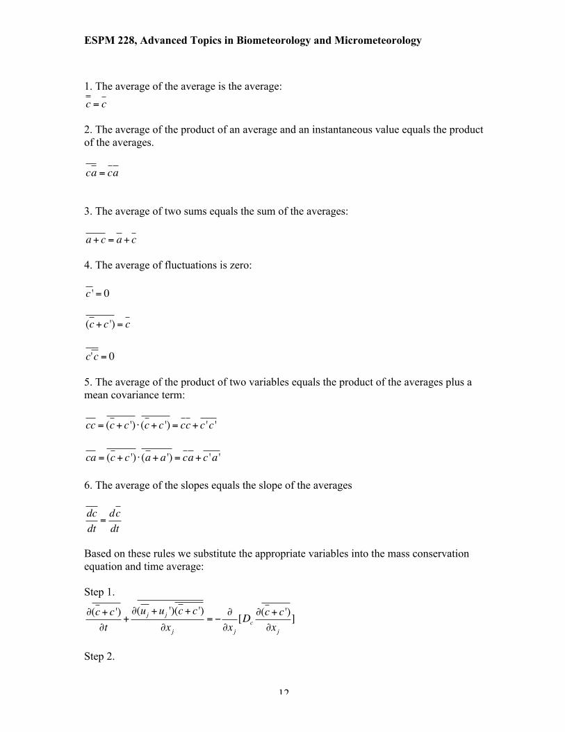
Based on these rules we substitute the appropriate variables into the mass conservation equation and time average: Step 1.

∂(c+ c ')∂t

+∂(uj +uj ')(c+ c ')

∂x j= −

∂∂x j[Dc

∂(c+ c ')∂x j

]

Step 2.


13

∂c∂t+∂cu j

∂x j+∂uj 'c '∂x j

= −∂∂x j[Dc

∂c∂x j]

Step 3. ∂c∂t+ c ∂u j

∂x j+u j

∂c∂x j

+∂uj 'c '∂x j

= −∂∂x j[Dc

∂c∂x j]

Applying the incompressible flow assumption reduces this equation to: ∂u j∂x j

= 0

Step 4. ∂c∂t+u j

∂c∂x j

+∂uj 'c '∂x j

= −∂∂x j[Dc

∂c∂x j]

We will see in later lectures that the principles of continuity and conservation of mass have application to other problems we will face, such as the conservation of energy, heat, turbulent kinetic energy and momentum. The covariance term, uj 'c ' , represents the turbulent flux density. It is one of the most important concepts in micrometeorology and as we will see later it is also the bane of fluid dynamics. This is a second order moment adds an additional unknown to the equation of mass. Its introduction vastly complicates the solution of the conservation equation for practical applications, and as a results the solution of this family of equations is one of the major unsolved problems of physics. This expression of the conservation of mass is valid at a point. It contains terms for time rate of change, advection, flux divergence and sources and sinks. To make practical use of the Equation one should integrate it over a control volume whose lower boundary consists of the interface between the air and the soil and vegetation and whose upper and lateral boundaries are fixed in the air.

For the simple case of steady state conditions (dc/dt = 0), horizontal homogeniety (no horizontal gradients) and no chemical reactions, this equation reduces to:

0 = −ρa∂w 'c '∂ z

+ SB (z)

Integrating this equation with respect to height yields the classic relationship, from micrometeorological theory is generally applied. We obtain a relation that shows that the eddy covariance between vertical velocity and scalar concentration fluctuations


14

(measured at a reference height, h) equals the net flux density of material in and out of the underlying soil and vegetation.

ρaw 'c '(h) = ρaw 'c '(0)+ S(z)dz0

h

∫

When the thermal stratification of the atmosphere is stable or turbulent mixing is weak, material leaving leaves and the soil may not the reference height h. Under such conditions the storage term becomes non-zero, so it must be added to the eddy covariance measurement if we expect to obtain a measure of material flowing into and out of the soil and vegetation.

ρaw 'c '(h)+ ρa∂s∂t0

h

∫ dt = ρaw 'c '(0)+ S(z)dz0

h

∫

While the storage term is small over short crops, it is an important quantity over forests. With respect to CO2, its value is greatest near sunrise and sunset when there is a transition between respiration and photosynthesis and a break-up of the stable nocturnal boundary layer by the onset of convective turbulence. With respect to the study of pollutants, the interception of a wandering plume can cause the storage term to deviate from zero. It is important to apply this equation in non-stationary conditions to avoid giving biological or physical interpretation to flux densities that are not local in time. A classic case involves the measure of CO2 flux density at sunrise. Often a large efflux is detected with the conventional eddy covariance method. This value has no biological support, for the efflux may be several times the magnitude of the potential respiration by the soil and vegetation. In actually, this flux density is real, but it represents the accumulation of respiration that has gone on for several hours in the dark. During night the boundary layer is stable and the forest environment is decoupled from the atmosphere. Thereby CO2 builds up in the canopy air space and is vented to the atmosphere only after sunrise when turbulent mixing resumes. Motivated by a need to circumvent this complexity, Lee [Lee, 1998] re-visited the budget equation (Equation 1) and applied it to the case of CO2 exchange. His goal was to derive an equation that could be used to assess fluxes under non-ideal conditions using conventional experimental instrumentation, mounted on a solitary tower. To do so, he assumed advection was non-negligible in the vertical and longitudinal directions.

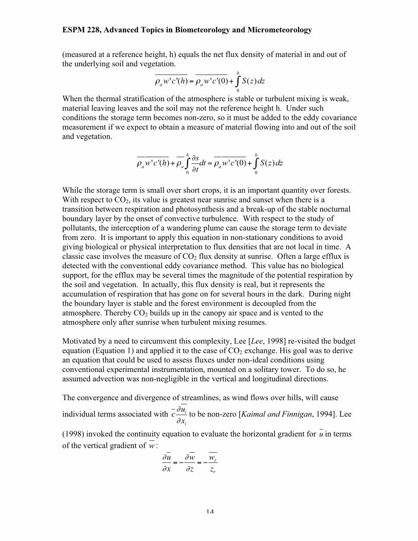
The convergence and divergence of streamlines, as wind flows over hills, will cause

individual terms associated with c∂ui∂xi

to be non-zero [Kaimal and Finnigan, 1994]. Lee

(1998) invoked the continuity equation to evaluate the horizontal gradient for u in terms of the vertical gradient of w :

∂u∂x

= −∂w∂z

= −wr

zr


15

The term, wr , is defined as a mean vertical velocity measured at the reference height, r. This mean vertical velocity should not be confused with the raw vertical velocity output of a sonic anemometer. On flat terrain, non-zero values ofwr , on the time scale of hours, arises from convection, synoptic scale subsidence or local circulating flows due to thermal [Lee, 1998]. Over complex terrain, drainage flows will cause wr to be non zero.

The other assumptions made by Lee [Lee, 1998] include:

∂u 's '∂x

= 0

u∂s∂x

= 0

w∂s∂z

+ s∂w∂z

=∂ws∂z

Following the assumptions made by Lee [Lee, 1998]an expression for net ecosystem exchange of CO2 (Ne) is derived. It equals the sum of the eddy covariance, measured at a reference height, the storage term and a parameterized ‘advection’ term.

Ne =

ρaw 's '(0)+ SB (z, t)dz0

h

∫ =

ρa w 's '(h)+∂s∂tdz

0

h

∫ + w∂s∂z

+ s∂w∂z

"

#$

%

&'

0

h

∫ dz"

#$

%

&'

Assessing the terms on the right-hand side yields:

Ne = ρa w 'c '(h)+∂c∂tdz

0

h

∫ +wr (cr− < c >)#

$%

&

'(

where, wr = w zr( ) and c =1zr

c0

zr∫ z( )dz .

The mean, vertical velocity at the reference height (wr ) is the difference between two other vertical velocities:

wr = w− w

Though Lee’s advection correction improves upon our interpretation of Ne, we cannot conclude that it is the definitive correction term for interpreting eddy covariance measurements over tall forests on complex terrain. Spatial variation in the mean flow and the scalar mixing ratio field, as a result of topography and changes in surface


16

roughness and biospheric source and sinks strengths, produces spatial variation in the mean turbulent fluxes that may not be accommodated by this one-dimensional relation.

In reality ∂u∂x

+∂v∂y

= −∂w∂z

So there has been movement from using the Lee equation and considering advection

in 2 dimensions. A simplified version reduces to:

ρa u∂s∂x+w ∂s

∂z!

"#

$

%&= −ρa

∂ "w s '∂z

!

"#

$

%&+ SB x, z, t( )

With regard to flow over a low hill, there are four mechanisms that can induce advective fluxes of scalars, such as CO2 and water vapor [Katul et al., 2006; Raupach and Finnigan, 1997].

One, horizontal gradients in carbon dioxide source-sink strengths will be generated along the direction of the wind passage by spatial variations in light, soil moisture, soil texture, leaf area and species composition. The radiant energy flux density to the soil and canopy is a function of the angle between the solar beam and the normal to an inclined surface. Radiation gradients along a hill impose direct spatial gradients on the surface energy balance, stomatal conductance, photosynthesis and respiration. Differential radiation interception along a hill can also generate streamwise differences in thermal stratification and atmospheric stability. On the longer term (season to years), the soil texture will vary from the top to the bottom of a hill, as will vegetation water use. This combination of interactions will affect the stature of vegetation, its physiological functioning and species composition.

Two, any change in surface roughness along the longitudinal axis of a hill will alter

the surface stress, friction velocity (u*) and the eddy exchange coefficient (Kx). This alteration, in turn, feeds the scalar flux boundary condition, as it is proportional to the product of the local eddy exchange coefficient and the scalar mixing ratio gradient, normal to the hill.

Three, as spatial variations in the turbulent stresses develop, in response to changes in

the mean windfield, they will generate spatial variation in the eddy fluxes of the scalar. This can be illustrated by considering the production terms of the relevant eddy flux rate equations. These terms typically take the form of the product of turbulent stresses and mean concentration gradients, !ui !uj ∂c ∂x j .


17

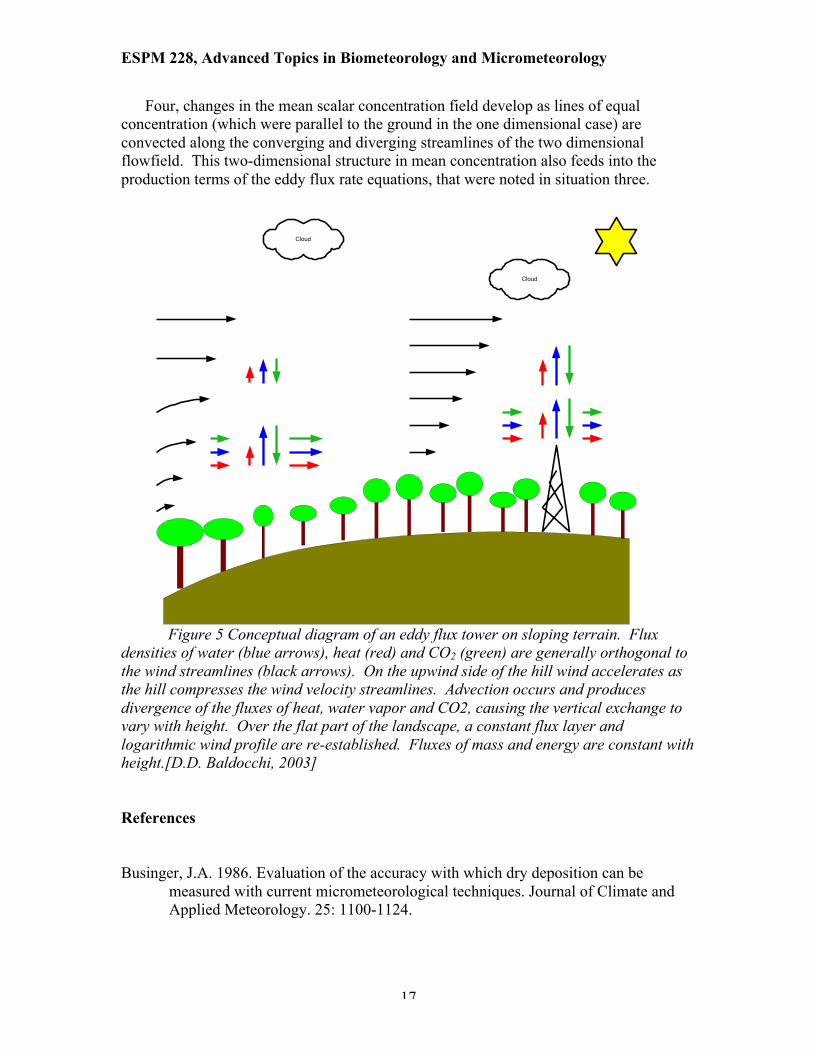
Four, changes in the mean scalar concentration field develop as lines of equal concentration (which were parallel to the ground in the one dimensional case) are convected along the converging and diverging streamlines of the two dimensional flowfield. This two-dimensional structure in mean concentration also feeds into the production terms of the eddy flux rate equations, that were noted in situation three.

Figure 5 Conceptual diagram of an eddy flux tower on sloping terrain. Flux

densities of water (blue arrows), heat (red) and CO2 (green) are generally orthogonal to the wind streamlines (black arrows). On the upwind side of the hill wind accelerates as the hill compresses the wind velocity streamlines. Advection occurs and produces divergence of the fluxes of heat, water vapor and CO2, causing the vertical exchange to vary with height. Over the flat part of the landscape, a constant flux layer and logarithmic wind profile are re-established. Fluxes of mass and energy are constant with height.[D.D. Baldocchi, 2003] References Businger, J.A. 1986. Evaluation of the accuracy with which dry deposition can be

measured with current micrometeorological techniques. Journal of Climate and Applied Meteorology. 25: 1100-1124.

Cloud

Cloud


18

Crawford, TL, RJ Dobosy, RT McMillen, CA Vogel and BB Hicks. 1996. Air-surface exchange measurements in heterogeneous regions: extending tower observations with spatial structure observed from small aircraft. Global Change Biology. 2, 275-286.

Denmead, O.T. 1983. Micrometeorological methods for measuring gaseous losses of

nitrogen in the field. In: Gaseous Loss of Nitrogen from plant-soil systems. eds. J.R. Freney and J.R. Simpson. pp 137-155.

Denmead, O.T. and M.R. Raupach. 1993. Methods for measuring atmospheric gas

transport in agricultural and forest systems. In: Agricultural Ecosystem Effects on Trace Gases and Global Climate Change. American Society of Agronomy.

Foken, Th. and B. Wichura. 1995. Tools for quality assessment of surface-based flux

measurements', Agricultural and Forest Meteorology, 78, 83-105. Fuehrer, P.L. and Friehe, C.A., 2002. Flux corrections revisited. Boundary Layer

Meteorology, 102: 415-457. Goulden, M.L., Munger, J.W., Fan, S.M., Daube, B.C. and Wofsy, S.C., 1996.

Measurements of carbon sequestration by long-term eddy covariance: Methods and a critical evaluation of accuracy. Global Change Biology, 2(3): 169-182.

Ham, J.M. and Heilman, J.L., 2003. Experimental Test of Density and Energy-Balance

Corrections on Carbon Dioxide Flux as Measured Using Open-Path Eddy Covariance. Agron J, 95(6): 1393-1403.

Horst, T.W. 1997. A simple formula for attenuation of eddy fluxes measured with first

order response scalar sensors. Boundary Layer Meteorology. 82, 219-233. Kaimal, J.C. and J.J. Finnigan. 1994. Atmospheric Boundary Layer Flows: Their

Structure and Measurement. Oxford University Press, Oxford, UK. 289 pp. Lenschow, DH. 1995. Micrometeorological techniques for measuring biosphere-

atmosphere trace gas exchange. In: Biogenic Trace Gases: Measuring Emissions from Soil and Water. Eds. P.A. Matson and R.C. Harriss. Blackwell Sci. Pub. Pp 126-163.

Massman, W.J. 2000. A simple method for estimating frequency response corrections for

eddy covariance systems. Agricultural and Forest Meteorology.104, 185-198. Massman, W.J. and Lee, X., 2002. Eddy covariance flux corrections and uncertainties in

long-term studies of carbon and energy exchanges. Agricultural and Forest Meteorology, 113(1-4): 121-144.


19

McMillen, R.T. 1988. 'An eddy correlation technique with extended applicability to non-simple terrain', Boundary Layer Meteorology, 43, 231-245.

Moncrieff, J.B., Y. Mahli and R. Leuning. 1996. 'The propagation of errors in long term

measurements of land atmosphere fluxes of carbon and water', Global Change Biology, 2, 231-240.

Moore, C. 1986. Frequency response corrections for eddy covariance systems. Boundary

Layer Meteorology. 37, 17-35. Raupach and Lenschow (sampling through a line) Suyker, A.E. and S.B. Verma. 1993. Eddy correlation measurement of CO2 flux using a

closed path sensor: theory and field tests against an open path sensor. Boundary-Layer Meteorology. 64, 391-407.

Swinbank, WC, 1951. The measurement of vertical transfer of heat and water vapor by

eddies in the lower atmosphere. Journal of Meteorology. 8, 135-145. Swinbank, W.C. 1955. An experimental study of eddy transport in the lower atmosphere.

Division of Meteorological Physics Technical Paper, 2. CSIRO. Melbourne. 29 pp.

Van den Hurk, B. 1996. Sparse canopy parameterizations for meteorological models.

Wageningen University. Webb, E.K., G. Pearman and R. Leuning. 1980. 'Correction of flux measurements for

density effects due to heat and water vapor transfer', Quarterly Journal of Royal Meteorological Society, 106, 85-100.

Wesely, M.L. 1970. Eddy correlation measurements in the atmospheric surface layer

over agricultural crops. Dissertation. University of Wisconsin. Madison, WI. Wesely, M.L., D.H. Lenschow and O.T. 1989. Flux measurement techniques. In: Global

Tropospheric Chemistry, Chemical Fluxes in the Global Atmosphere. NCAR Report. Eds. DH Lenschow and BB Hicks. Pp 31-46.

Endnote References Aubinet, M., et al. (2000), Estimates of the annual net carbon and water exchange of Europeran forests: the EUROFLUX methodology, Advances in Ecological Research, 30, 113-175.


20

Baldocchi, D. D. (2003), Assessing the eddy covariance technique for evaluating carbon dioxide exchange rates of ecosystems:past, present and future., Global Change Biol, 9, 479-492. Baldocchi, D. D., B. B. Hicks, and T. P. Meyers (1988), Measuring biosphere-atmosphere exchanges of biologically related gases with micrometeorological methods, Ecology., 69, 1331-1340. Finnigan, J. J., R. Clement, Y. Malhi, R. Leuning, and H. A. Cleugh (2003), A Re-Evaluation of Long-Term Flux Measurement Techniques Part I: Averaging and Coordinate Rotation, Boundary Layer Meteorology, 107, 1-48. Fuehrer, P. L., and C. A. Friehe (2002), Flux corrections revisited, Boundary Layer Meteorology, 102, 415-457. Gu, L., W. J. Massman, R. Leuning, S. G. Pallardy, T. Meyers, P. J. Hanson, J. S. Riggs, K. P. Hosman, and B. Yang (2012), The fundamental equation of eddy covariance and its application in flux measurements, Agricultural and Forest Meteorology, 152(0), 135-148. Ham, J. M., and J. L. Heilman (2003), Experimental Test of Density and Energy-Balance Corrections on Carbon Dioxide Flux as Measured Using Open-Path Eddy Covariance, Agron J, 95(6), 1393-1403. Kaimal, J. C., and J. J. Finnigan (1994), Atmospheric Boundary Layer Flows, 302 pp., Oxford University Press. Katul, G. G., J. J. Finnigan, D. Poggi, R. Leuning, and S. E. Belcher (2006), The influence of hilly terrain on canopy-atmosphere carbon dioxide exchange, Boundary-Layer Meteorology, 118(1), 189-216. Lee, X. (1998), On micrometeorological observations of surface-air exchange over tall vegetation, Agricultural and Forest Meteorology, 91(1-2), 39-49. Leuning, R. (2007), The correct form of the Webb, Pearman and Leuning equation for eddy fluxes of trace gases in steady and non-steady state, horizontally homogeneous flows, Boundary-Layer Meteorology, 123(2), 263-267. Leuning, R., and J. Moncrieff (1990), Eddy-Covariance Co2 Flux Measurements Using Open-Path and Closed-Path Co2 Analyzers - Corrections for Analyzer Water-Vapor Sensitivity and Damping of Fluctuations in Air Sampling Tubes, Boundary-Layer Meteorology, 53(1-2), 63-76. Leuning, R., O. T. Denmead, A. R. G. Lang, and E. Ohtaki (1982), Effects of Heat and Water-Vapor Transport on Eddy Covariance Measurement of CO2 Fluxes, Boundary-Layer Meteorology, 23(2), 209-222. Liu, H. (2005), An Alternative Approach for CO<sub>2</sub> Flux Correction Caused by Heat and Water Vapour Transfer, Boundary-Layer Meteorology, 115(1), 151-168. Massman, W. J., and X. Lee (2002), Eddy covariance flux corrections and uncertainties in long-term studies of carbon and energy exchanges, Agricultural and Forest Meteorology, 113(1-4), 121-144. Pattey, E., G. Edwards, I. B. Strachan, R. L. Desjardins, S. Kaharabata, and C. W. Riddle (2006), Towards standards for measuring greenhouse gas fluxes from agricultural fields using instrumented towers, Canadian Journal of Soil Science, 86(3), 373-400. Paw U, K. T., D. D. Baldocchi, T. P. Meyers, and K. B. Wilson (2000), Correction of eddy covariance measurements incorporating both advective effects and density fluxes, Boundary Layer Meteorology. 97, 487-511.


21

Raupach, M. R., and J. J. Finnigan (1997), The influence of topography on meteorological variables and surface-atmosphere interactions, Journal of Hydrology, 190(3-4), 182-213. Reynolds, O. (1895), On the dynamical theory of incompressible viscous fluids and the determinatino of the criterion, Philosophical Transactions of the Royal Society of London, A, 186, 123-164. Webb, E. K., G. I. Pearman, and R. Leuning (1980), Correction of Flux Measurements for Density Effects Due to Heat and Water-Vapor Transfer, Q. J. R. Meteorol. Soc., 106(447), 85-100.

lecture 3 notes espm 228 micromet flux measurements eddy...

Documents