Munich Personal RePEc Archive

Learning and heterogeneity in GDP and

inflation forecasts

Lahiri, Kajal and Sheng, Xuguang

Department of Economics, University at Albany, NY, 12222,

Department of Economics, SUNY Fredonia, NY, 14063

2009

Online at https://mpra.ub.uni-muenchen.de/21448/

MPRA Paper No. 21448, posted 18 Mar 2010 18:25 UTC

1

Learning and Heterogeneity in GDP and Inflation Forecasts*

Kajal Lahiri**

Department of Economics, University at Albany - SUNY Albany, NY 12222, United States

Xuguang Sheng

Department of Economics, SUNY Fredonia Fredonia, NY 14063, United States

Abstract: We estimate a Bayesian learning model with heterogeneity aimed at explaining the evolution of expert disagreement in forecasting real GDP growth and inflation over 24 monthly horizons for G7 countries during 1990-2007. Professional forecasters are found to begin and have relatively more success in predicting inflation than real GDP at significantly longer horizons; forecasts for real GDP contain little information beyond 6 quarters, but forecasts for inflation have predictive value beyond 24 months and even 36 months for some countries. Forecast disagreement arises from two primary sources in our model: differences in the initial prior beliefs of experts, and differences in the interpretation of new public information. Estimated model parameters, together with two separate case studies on (i) the dynamics of forecast disagreement in the aftermath of the 9/11 terrorist attack in the U.S. and (ii) the successful inflation targeting experience in Italy after 1997, firmly establish the importance of these two pathways to expert disagreement.

Key words: Bayesian learning, Public information, Panel data, Forecast disagreement, Forecast horizon, Content function, Forecast efficiency, GDP, Inflation targeting.

JEL classification: C11; E17

* An earlier version of this paper was presented at the 28th International Symposium on Forecasting (2008). We thank Frank Diebold, David Hendry, Lars-Erik Öller, Mark Watson and participants of the symposium for many helpful comments and suggestions. However, we alone are responsible for any remaining errors and shortcomings. ** Corresponding author. Tel.: +1 518 442 4758; fax: +1 518 442 4736. E-mail addresses: klahiri@albany.edu (K. Lahiri), sheng@fredonia.edu (X. Sheng).

2

1. Introduction

Various survey data on expectations from many countries over last few decades

have produced mounting evidence on substantial inter-personal heterogeneity in how

people perceive the current and form inferences about the future economic conditions.1

Lucas (1973) attributed the observed disagreement to individuals having exposed to

different information sets, whereas in Carroll (2003) and Mankiw et al. (2003)

disagreement arises because agents update new information only occasionally. While

analyzing the diverse behavior of professional forecasters, Kandel and Pearson (1995)

and Kandel and Zilberfarb (1999) have produced some startling evidence that agents not

only have differential information sets, but may also interpret the same public

information differentially. Heterogeneity in processing information and lack of common

beliefs is a central theme that has emerged in many areas of economics; see Acemoglu et

al. (2006).

Based on monthly fixed-target forecast data for real GDP, Lahiri and Sheng

(2008) estimated a Bayesian learning model with agent-specific heterogeneity aimed at

explaining the role of initial priors in forecast disagreement and its evolution over

horizons. By studying the term structure of forecast disagreement, one learns a great deal

about the importance of initial prior beliefs, the timing of information arrival and the

efficiency in the use of public information. We found experts to start off with widely

divergent initial prior beliefs at very long horizons. Their initial beliefs propagate forward

onto the whole series of forecasts, generating significant amount of inertia in expectations

formation. The diversity in initial beliefs explained nearly 100% to 30% of forecast

1 See Jonung (1981), Zarnowitz and Lambros (1987), Maddala (1991), Souleles (2004), Patton and Timmermann (2007), and Capistrán and Timmermann (2008), among many others.

3

disagreement as the horizon decreases from 24 months to 1 month. This “anchoring” like

effect, much emphasized in the psychological literature, is a result of optimal Bayesian

information processing in the presence of initial priors, see Tversky and Kahneman

(1974) and Zellner (2002).

In this paper we extend our analysis to both real GDP and inflation forecasts using

more recent data, and highlight certain important differences in the way professional

forecasters treat these two variables in producing multi-period forecasts. We use forecasts

for seven industrialized countries during 1990-2007. Compared to real GDP, we found

the professional forecasters to (i) disagree less about the future inflation, (ii) start

reducing their inflation forecast disagreement at significantly longer horizons, (iii) start

making meaningful forecast revisions about inflation much earlier, and (iv) tend to make

smaller forecast errors in inflation at all observed horizons.2 Also, (v) forecasts for real

GDP beyond 6 quarters contain very little information compared to conventional

benchmarks; however, forecasts for inflation have predictive value beyond 24 months

and even 36 months for some countries. These findings show that, compared to GDP,

professional forecasters begin to put more efforts and succeed in predicting inflation at

significantly longer horizons. At least a part of the explanation has to lie in the data

generating processes of the two target variables, and the fact that real GDP is inherently

more difficult to forecast than inflation.3 But the relative success in inflation forecasting

in recent years and the diminished disagreement can also be attributed to better anchoring

2 Note that these results are true for countries with and without inflation targeting, and also in earlier periods. Zarnowitz and Braun (1993) reported significantly smaller forecast errors for inflation compared to real GDP during the 1978-1990 period too. 3 It can also be determined partly by the demand side of the forecasting market, i.e., the society’s need for earlier and more credible inflation forecasts.

4

of long-run forecasts due to the central bank policy of inflation targeting that has been

officially adopted by some of the countries in our sample. Using the Bayesian learning

model, our study aims to identify the relative importance of alternative pathways through

which the policy authorities have achieved such objectives. Indeed, we find evidence that

suggests that due to better communication strategies and enhanced credibility of central

banks in forecast targeting in recent years (i) the diversity in the initial prior beliefs has

lessened, (ii) agents attach higher weights to public information and less to initial prior

beliefs while updating forecasts, and (iii) they incorporate new public information more

efficiently in forecasting inflation.

The paper is organized as follows. Section 2 presents some stylized facts based on

the cross-country forecast data. Section 3 estimates the Bayesian learning model and

presents empirical evidence on alternative pathways to forecast disagreement. This

section also presents two case studies on (i) the dynamics of forecast disagreement after

the 9/11 terrorist attack in the U.S. as a natural experiment, and (ii) the inflation targeting

experience in Italy after 1997. Section 4 investigates forecast efficiency in utilizing

public information for both real GDP and inflation. Section 5 explores the forecast

content functions to explain why forecasters find real GDP more difficult to forecast than

inflation. Section 6 concludes.

2. Some stylized facts

This section starts with a brief introduction of the data used in our analysis. We

then highlight a few stylized facts concerning the evolution of consensus forecasts,

forecast disagreement and forecast revisions in real GDP and inflation. We find some

5

important differences in the way professional forecasters treat these two macroeconomic

variables.

2.1 Data

The data for this study are taken from “Consensus Forecasts: A Digest of

International Economic Forecasts”, published by Consensus Economics Inc. We study a

panel of forecasts of annual real GDP growth and inflation. Inflation is measured by the

annual percentage change in consumer price index for all G7 countries except the United

Kingdom.4 The survey respondents start forecasting in January of the previous year, and

their last forecast is reported at the beginning of December of the target year. So for each

country and target year, we have 24 forecasts of varying horizons. Our data start with the

January 1990 forecasts and end with the December 2007 forecasts, giving predictions for

17 target years 1991 - 2007 and for seven major industrialized countries – Canada,

France, Germany, Italy, Japan, the United Kingdom and the United States.5 The number

of institutions ranges from 20 to 40. The forecasting institutions are typically banks,

securities firms, econometric modelers, industrial corporations and independent

forecasters. Since most of the institutions are located in the country they are forecasting

upon, country-specific expertise is guaranteed. Altogether we have more than 115,000

forecasts for GDP and inflation. In the following analysis, we use an early announcement

as the actual value, which is published in the May issues of Consensus Forecasts

immediately following the target year.

4 As a measure of UK price inflation, forecasters were asked about the annual percentage change in the retail price index. However, in line with the focus of Bank of England, from April 1997 onwards, forecasts are required instead for the retail price index excluding mortgage interest costs. 5 Note that the target for GDP and inflation in Germany changes in our data sample due to unification. We used forecasts for West Germany made for the target years 1991-1995, and for unified Germany for the target years 1996-2007.

6

For the current study, this data set has many advantages over some other more

commonly used surveys. First, Consensus Forecasts are regularly sold in a wide variety

of markets. Also, the names of the respondents are published next to their forecasts.

Hence one would expect these professional forecasts to satisfy a certain level of accuracy

in contrast to laymen expectations, as poor forecasts damage their reputation. Second,

since the importance of private information in forecasting GDP and inflation is expected

to be very small compared to such variables as corporate earnings, company stock prices,

etc., we can identify the news to GDP and inflation as mostly public information. Finally,

forecasts for fairly long horizons, currently from 24- to 1-month ahead, are available.

This fixed-event scheme enables us to study the role of heterogeneity in initial priors and

their revisions on expert disagreement for a sequence of 24 forecasts for 17 target years.

2.2 Evolution of consensus forecasts

Figure 1a presents the consensus (i.e. mean) forecasts and the realized actual

values of real GDP between 2003 and 2007.6 Plots start when the forecast horizon is 24,

which is reported in January of the previous year, and end when the forecast horizon is 0,

which gives the actual realization. Similar graphs for inflation for the extended period

1991 – 2007 are presented in Figure 1b.

First, note that for the first few rounds of forecasting (for horizons 24 to 18

months), for majority of the years and countries, the consensus forecasts do not seem to

change very much. This empirical observation leads us to believe that over these

horizons, forecasters do not receive much dependable information to revise their forecasts

systematically. Second, the initial 24-month ahead forecasts for all countries seem to be

6 Similar graphs for the evolution of real GDP consensus forecasts for the earlier years, i.e., 1991-2002 can be found in Isiklar and Lahiri (2007).

7

starting from a relatively narrow band and then as information is accumulated they tend

to diverge from these initial starting points and move towards their final destinations. One

may conjecture that these initial long-term forecasts are nothing but unconditional means

of the respective processes. Note also that the initial inflation forecasts seem to be

bunched together more than the initial GDP forecasts, and have become less variable

during 1991-2007 − more for some countries than others.

All in all, a close look at these graphs reveals certain regularities on how the

fixed-target consensus forecasts evolve over time. The variability of mean forecasts over

the target years is very small at the longer horizons, and increases rapidly as the forecast

horizon gets shorter. We now proceed to examine more rigorously the underlying

dynamics in forecaster disagreement around these consensus forecasts and timing of the

arrival of important information when forecasters break away from their initial estimates.

2.3 Evolution of forecast disagreement

Following the literature, we measure forecast disagreement as the variance of

forecasts across professional forecasters.7 For each country, we calculate forecast

disagreement separately for each target year and horizon, and find them to vary

dramatically over time and across horizons. The results imply that occasionally the

economies go through substantial changes that are very difficult to forecast by virtually

any of the techniques currently used to forecast economic variables. We merely observe

that heterogeneity of expectations is the norm in the market place.

In order to study the general pattern of forecast disagreement over horizons, we

plot the average disagreement over 17 target years at each of the 24 forecast horizons for

7 In our study sample where only more frequent respondents were included, the inter-quartile range and variance of individual forecasts were found to be very similar, cf. Döpke and Fritsche (2006).

8

GDP and inflation forecasts in Figure 2. Like before, plots start when the horizon is 24

months and end when the horizon is 1 month. Although the magnitude of the

disagreement varies a lot across countries (France, Italy and Germany have

comparatively low disagreements), the extent of disagreement among professional

forecasters is less on the average in predicting inflation than GDP.8 For GDP forecasts,

the disagreement at the 24-month horizon is very high and stays almost unchanged or

declines only slightly till about the 16-month horizon; thereafter it starts to decrease

sharply at 15-month horizon and keeps declining as the horizon gets shorter. For inflation

forecasts the disagreement is also high at the beginning, but unlike real GDP, declines

monotonically as the horizon gets shorter from 24 months to 1 month.

2.4. Panel data analysis of forecast revisions

With fixed-target forecasts, an analysis of forecast revisions reveals important

information about when major public information arrives and how much experts interpret

them differently. Let ithF be the forecast of the target variable made by agent i, for the

target year t, and h months ahead of the end of the target year. Forecast revision is

defined as the difference between two successive forecasts for the same individual i and

the same target year t, i.e. 1+−=ithithith

FFR . The decomposition of the total sum of

squares in our panel data on forecast revisions into between- and within-agent variations

can reveal important characteristics of forecasts. In this context, we introduce three

measures, within-agent variation (w

hS ), between-agent variation (

b

hS ) and total variation

8 Note that for UK, if we ignore the initial two years and 1994-96 during which the definition of the price variable was changed, the disagreement at h=24 will be much smaller than that for real GDP.

9

(t

hS ) in forecast revisions at each horizon, adjusted for the number of forecasters,

respectively,

∑∑∑== =

−=hh ih N

i

ih

N

i

T

t

hiith

w

h TRRS11 1

2. /)(

(1)

∑∑==

−=hh N

i

ih

N

i

hhiih

b

h TRRTS11

2... /)(

(2)

∑∑∑== =

−=hh ih N

i

ih

N

i

T

t

hith

t

h TRRS11 1

2.. /)(

(3)

where ∑=

=ihT

t

ihithhi TRR1

. / is the mean forecast revisions over time and ∑=

=hN

i

hhih NRR1

... / the

overall mean revisions over time and across agents. Since not all forecasters responded at

all times, we have to deal with the unbalanced panel by taking summation over different

time and horizons. Forecasters who responded less than 10% of the times are deleted

from our forecast revision analysis such that our results are not dominated by very few

extreme observations. By construction, the total variation in forecast revisions is the sum

of within-agent and between-agent variation, that is, .b

h

w

h

t

hSSS +=

Tables 1a and 1b show the ratio of between-agent variation to total variation in

GDP and inflation forecast revisions, respectively. Depending on the horizon and country

we consider, between-agent variation explains 4% to 34% of the total variation in

forecast revisions. Over all horizons, between-agent variation accounts for 10%-15% of

the total variation in GDP and 12%-17% in inflation forecasts on the average. We take

this as the first evidence that professional forecasters on some occasions interpret the

same public signal quite differently. The between-agent variation, however, is relatively

small, since total variation in forecast revision is mainly driven by within-agent variation.

10

This is not unexpected because our forecasters are professional experts, and the targets

are widely discussed macroeconomic entities.

Because of its relative size, we should also be interested in the evolution of

within-agent variation over horizons, which shows how professional forecasters revise

their forecasts intra-personally after observing new public signals each month. Figures 3a

and 3b plot the total variation and its components in GDP and inflation forecast revisions,

respectively. Whenever we see a big jump in within-agent variation at a certain horizon,

it means professional forecasters make major revisions at that specific horizon.

For GDP forecasts, the first big spike is observed at horizon 15 months for all

sampled countries, which simply suggests that professional forecasters observe the first

relevant public signal and revise their forecasts at the beginning of October of the

previous year. Depending on the timing of their base-year GDP announcements, within-

agent variation gets a boost again at horizons 11 to 9 months, which, as expected, affects

the forecasts for year-over-year growth rate. As forecast horizon declines, within-agent

variation gets a boost whenever the first release of GDP growth for the previous quarter

becomes available.9

As for inflation forecasts, we also observe a big spike in within-agent variation

around horizon 15 months for all sampled countries. It is remarkable that for both

9 For the US, within-agent variation jumps at horizons 8 and 5 months as a result of the advance release of first quarter GDP growth at the end of April and second quarter GDP growth at the end of July, respectively. For Canada, France and Germany, within-agent variation jumps at horizons 7 and 4 months with the release of first quarter GDP growth at the end of May and second quarter GDP growth at the end of August, respectively. For Italy and Japan, within-agent variation peaks at horizons 6 and 3 months, since their first and second quarter GDP growth figures are released at the end of June and September, respectively. For the UK, within-agent variation peaks at horizon 6 months since the complete estimate of first quarter GDP is not available until the end of June, which is 3 months after the end of first quarter.

11

inflation and real GDP, a substantial forecast revision takes place at this horizon.10

However, for inflation, professional forecasters start making major forecast revisions

much earlier, which are discernible at horizon 22 months for Canada, Germany and UK

and 18 months for other G7 countries except Italy, which has its highest peak at the 15-

month horizon. Recent research by Banerjee and Marcellino (2006), Gürkaynak et al.

(2007) and others have documented that monthly indicators such as capacity utilization,

consumer confidence, industrial production, new home sales, initial job claims, leading

indicators, purchasing managers’ index, nonfarm payroll, retail sales, unemployment,

business tendency surveys, and numerous others are regularly utilized by market

forecasters to gauge future expectations.

As the horizon gets shorter, within-agent variation gets boosts whenever some

relevant information becomes available concerning inflation for the target year, including

quarterly IPD announcements, various monthly variables and leading indicators. But it is

interesting to note that even for inflation forecasters do not seem to revise forecasts

uniformly on a monthly basis. This gives some credence to the hypothesis put forward by

Mankiw et al. (2003) that forecasts are not updated on a continuous basis.

Nevertheless, our evidence suggests that professional forecasters get more active

and succeed in forecasting inflation than real GDP growth beginning at much longer

horizons. This is also corroborated in Figure 4 where we have plotted the root mean

squared forecast errors (RMSE) for real GDP and inflation based on our Consensus

Forecasts individual data set during 1991-2007. We find that RMSE for real GDP at

horizons 24-18 months stays relatively flat, but for inflation it slowly but steadily

10 One might have thought that the most important revision would take place at around h=11 when the last year’s actual value is known, cf. Patton and Timmermann (2007).

12

declines from the beginning (i.e. h=24).11 To understand this interesting phenomenon,

one has to explore the underlying data generating process for the target variables, and

also keep in mind that forecasters find many other indicators useful for macro prediction

in real life. This possibility is formally explored in section 5.

3. Why do forecasters disagree?

This section begins with a simple Bayesian information updating model to explain

the stylized facts we have established so far. We then estimate the deep model parameters

using panel data. At the end of section, we identify the contribution of each component in

explaining forecast disagreement.

3.1 The Bayesian updating model

In section 2 we have seen that in predicting real GDP, professional forecasters do

not seem to adjust their initial forecasts much and sustain their original disagreement

during the initial rounds of forecasting.12 We also noted that at long horizons, consensus

(mean) forecasts vary very little over time implying that the idiosyncratic components in

each year’s forecasts cancel out while averaging over forecasters. Our Bayesian model

explicitly recognizes these twin facts and hypothesizes that professional forecasters begin

forecasting with specific prior beliefs at the 24-month horizon. Even though 24-month

ahead forecasts are strictly medium-run forecasts, there is some evidence that suggests

that these forecasts are in fact very close to being long-run forecasts. In Figures 5a and 5b

we have pitted 10-year forecasts of real GDP and inflation respectively for US obtained

11 These findings are consistent with a larger forecasting literature that has reported larger errors associated with GDP forecasts compared to inflation, see, for example, Zarnowitz and Braun (1993), Öller and Barot (2000), Blix et al. (2001), Stock and Watson (2003) and Banerjee and Marcellino (2006) over various sample periods and countries. 12 In case of inflation, meaningful updating seems to begin at horizons slightly longer than 24 months. More evidence on this will issue come up later.

13

from the Survey of Professional Forecasters (SPF) of Philadelphia Federal Reserve Bank

against 24-month ahead forecasts from our Consensus Forecasts database during 1992-

2006. The corresponding disagreements are also reported.13 Even though, as expected,

the variations in 10-year long-run expectations are slightly muted, the two series are

remarkably similar in terms of mean values of forecasts and the disagreement measures.14

Accordingly, following Lahiri and Sheng (2008), we make the following specific

assumption about forecasters’ initial or long-run prior beliefs.

Assumption 1:

The initial prior belief of the target variable for the year t, held by the forecaster i,

at the 24-month horizon is represented by the normal density with the mean 24itF and the

precision (i.e. the reciprocal of the variance) 24ita for ,,...,1 Ni = .,...,1 Tt = 15

In thinking about why professional forecasters disagree regarding their long-run

forecasts, note that a wealth of historical information on GDP and inflation are publicly

available to all forecasters to estimate the long-run unconditional values of the series.

Thus, it is not the availability of relevant data but the models, methods and philosophies

used to interpret them that are different from one forecaster to another. This is consistent

with the findings in Döpke and Fritsche (2006) that forecasters do not share a common

belief about what is an adequate model of the economy. For instance, some are neo-

Keynesians and some may be monetarists. To a certain extent, persistent diversity is also

13 To match the timing of forecasts we compare the February forecasts of Consensus Forecasts with first quarter forecasts from SPF (that are reported in the middle of the quarter). 14 Given that the two surveys are conducted independently on different groups of forecasters, this result is quite remarkable. A similar conclusion regarding the long-run and 24-month ahead expectations (and disagreement) in the euro area can be drawn based on ECB SPF, see Bowles et al. (2007). 15 The precisions of initial prior beliefs are allowed to be different across forecasters. This assumption is confirmed by the recent studies using density forecasts that document the heterogeneity in forecast uncertainty, see, for example, Lahiri and Liu (2006), Bowles et al. (2007), and Boero et al. (2008).

14

generated depending on the specific past sample that one uses to compute the

unconditional means. Due to the length of the forecasting horizon, experts face very high

uncertainty in interpreting available information based on whatever model or judgment

they are using, and hence disagree a lot about GDP and inflation in the long- or medium-

run.

An important implication of this assumption is that there will typically be an

“agreement to disagree” between professional forecasters. In other words, given their

divergent initial beliefs, forecasters will agree that, after seeing the same public signals

year after year, they will continue to disagree in their outlooks. This evidence is

consistent with the theoretical prediction in Acemoglu et al. (2006) who showed that,

starting with heterogeneous prior beliefs, agents may not converge to a consensus even

after observing the same infinite sequence of signals when there is a lot of uncertainty in

the public information. This is interesting because the common prior assumption,

typically made in the old learning literature, leads to the well-known no “agreement to

disagree” result (cf. Aumann, 1987).

With the arrival of new public information, experts progressively learn over

horizons to modify their initial beliefs. Consistent with our broad empirical findings on

the fixed-target forecasts, we make the following assumption concerning information

arrival.

Assumption 2:

At horizon h months, forecasters receive public signal thL concerning the target

variable but may not interpret it identically. In particular, individual i’s estimate of the

15

target variable, ithY , conditional only on the new public signal that is observed at forecast

horizon h months, can be written as

iththithLY ε−= , ),(~

ithithithbN µε . (4)

Assumption 2 allows for the possibility that agents can interpret the same public

signal differently, which is captured by ithµ with associated uncertainty ith

b . At each

month, all agents observe a new public signal but disagree on its effect on GDP and

inflation for the target year. One expert can interpret the signal more optimistically or

pessimistically than another. The precision of public information ithb allows individual

forecasters some latitude in interpreting public signals, and is a key parameter in

generating expert disagreement. Assumption 2 is in line with the empirical evidence

presented above about significant between-agent variation in forecast revisions, and also

with a large finance literature that equally informed agents can interpret the same

information differently (cf. Varian, 1989; Harris and Raviv, 1993; Kandel and Pearson,

1995; Dominitz and Manski, 2005).

The Bayes rule implies that under the normality assumption, the posterior mean is

the weighted average of the prior mean and the likelihood:

))(1(1 iththithithithithLFF µλλ −−+= + , (5)

where )/( 11 ithithithithbaa += ++λ is the weight attached to prior beliefs. For convenience,

the following population parameters are defined across professional forecasters for target

year t at horizon h months: thF and

2thF

σ are the mean and variance of forecasts of the

target variable; thλ and 2

thλσ are the mean and variance of the population distribution of

the weights attached to prior beliefs; and thµ and 2

thµσ are the mean and variance of the

16

population distribution of interpretation of public information. Under the simplifying

assumption that 1+ithF , ith

λ and ithµ are mutually independent of each other for any t and

h, one can derive the following relationship between disagreement in two consecutive

rounds of fixed-target forecasting:

222222221

2 )]1/([])1([)( thththththththththFthFF λσλσσλσσσ λλµλ −∆+−+++= + . (6)

In (6) the dynamics of forecast disagreement over horizons is seen to be governed by

three deep parameters of the model representing across-forecaster differences in (i) prior

beliefs, 2

1+thFσ ; (ii) the weights attached to priors,

2thλσ and (iii) the interpretation of

public signals, 2

thµσ . It encompasses a number of special cases. In one case where all

agents attach the same weight to their prior beliefs (i.e. 02 =thλσ for any t and h), (6)

becomes

2221

22 )1(thththFththF µσλσλσ −+= + . (7)

Our model suggests the following scenario of expectation formation by

professional forecasters. At the beginning of forecasting rounds, agents hold divergent

initial prior beliefs about the target variable in the long or medium run. Starting from

horizon h months, agents observe the same public signal but interpret it differently from

one another. Each agent then forms a new posterior distribution by combining his prior

and perception of the new public information using the Bayes rule. At horizon 1−h

months, each agent combines his updated prior belief, which is the posterior formed at

horizon h months, and his perception of new information, which is observed during the

current month, to derive the new posterior. The process continues until the end of

forecasting exercise for that target year. This cycle of prior to posterior is actually a very

17

solid way of characterizing the forecasting process: forecasters take what knowledge they

have in hand and update it with the arrival of new information (cf. El-Gamal and Grether,

1995).

3.2 Decomposition of forecast disagreement

Let us first focus on estimating one of our structural parameters - the relative

weight attached to prior belief ( hλ ). Equation (5) shows that

ithithithithFF ελ += +1 , (8)

where ))(1(iththithith

L µλε −−= is the error term. In estimating the above equation, several

econometric issues arise. First, note that (8) is not estimable, since the number of

parameters to be estimated exceeds the number of observations. We assume

ihhihithv+== λλλ , (9)

where ihv has mean zero, mutually independent of each other, and independent over

forecast horizons. We regress the forecast revision ( ithF∆ ) on the lagged forecast ( 1+ith

F )

to circumvent the possible problem of spurious regression. Thus, the estimable version of

(8) becomes

ithithhithuFF +=∆ +1β , (10)

where 1−=hh

λβ and 1++=ithihithith

Fvu ε . Second, as expected, ithu might be cross-

sectionally correlated due to common aggregate shocks. Following the line of reasoning

in Pesaran (2006), the common effects in the residuals are approximated by adding

additional variables 1+thF , th

F∆ and 1+∆th

F with the assumption that ithu is serially

correlated of order one in this augmented specification. Third, it may seem desirable to

estimate the panel data model in (10) with all three dimensions by imposing some smooth

18

functional form for hβ over horizons as in Gregory and Yetman (2004). See also Gregory

et al. (2001). However, as shown later, the estimated β varies unevenly over horizons,

depending on the lumpiness and timing of public information arrival. Thus, we estimated

(10) separately for each horizon, augmented by a few additional regressors to filter out

the effects of the cross-section correlation and serial correlation in the residuals:

ithithhithhithzcFF ηβ ++=∆ +1 , (11)

where ),,,,1( 111 +++ ∆∆∆=iththththith

FFFFz and 2

)(''' )( ihtiithE ησηη = , for ',',' hhttii === and

0 otherwise.

Tables 2a and 2b present the estimated weights attached to public information for

GDP and inflation forecasts respectively. In predicting both real GDP and inflation,

forecasters give a lower weight to public information at longer horizons because of its

low perceived quality, and a higher weight at short horizons as it becomes more precise.

At longer horizons, initial priors are relatively more important. Another important

observation is that, on average over all horizons, professional forecasters attach a higher

weight to public information in predicting inflation than GDP. Recall that from (5), the

relative weight attached to public information is a function of the precisions of new

information and prior beliefs, that is, 1

1

1 /1

/1

+

+

+ +=

+=−

ithith

ithith

ithith

ithith

ab

ab

ba

bλ . It immediately

follows that the ratio of the precision of new information to the precision of prior belief,

1/ +ithith ab is higher, and thus public information is perceived to be more precise and

certain in predicting inflation than GDP. This finding could possibly be explained by the

fact that initial GDP announcements are more heavily revised than price indexes,

observed only quarterly and involve substantial measurement errors. For instance, the

19

retail price index for the United Kingdom is never revised after its initial release. Also,

more frequent communication of the latest inflationary developments to the general

public and the commitment to long-run price stability by central banks may help to make

adjustments to inflationary expectations dependent more on current news.

Recall that forecast disagreement is posited to have three components, see

equation (6). Lahiri and Sheng (2008) find that the second component, i.e. differences in

the weights attached by experts to their prior beliefs, to barely have any effect on GDP

forecast disagreement, since professional forecasters place very similar weights on their

prior beliefs.16 We thus maintain a more parsimonious model (7) in which forecast

disagreement arises from two possible sources: differences in their initial prior beliefs,

and differences in their interpretation of public information. Substituting hλ̂ into (7), we

get estimates for the heterogeneity parameter in the interpretation of public signals,2

hµσ ,

as the sample average. Note that the differences in interpreting pubic information affect

forecast disagreement only through its interaction with the weight attached to public

information.

With the estimates of parameters in hand, we can check how well the

disagreement predicted by our model matches the disagreement observed in the survey

data. Substituting the parameter estimates of h

λ and 2hµσ into

( )∑ ∏∏+=

−

==

−

+−+=

23

1

221

22223

224

22 1)1(hj

tjtj

j

hs

tsthth

hj

tFtjthF µµ σλλσλσλσ , (12)

we get the dynamically generated forecast disagreement at each horizon that is predicted

by our model.

16 This component, however, might account for a large part of the disagreement in laymen’s expectations.

20

We find that, depending on the country, our estimated model explains from about

20% to 56% of the total variation in observed GDP forecast disagreement over all target

years and horizons. The corresponding figures for inflation forecasts are much higher,

ranging from 40% to 74%.17 It is interesting to note that using a dynamic structural time

series model with measurement errors and assuming forecast efficiency, Patton and

Timmermann (2007) could mimic the dispersion in the term structure of US real GDP

forecasts successfully, but not of inflation at the short horizons. We faced a similar

problem only for Italy’s inflation forecast dispersion at very short horizons. Note,

however, that the dispersion values for Italy are extremely low at short horizons, and

hence they need very little explaining. Considering the fact that forecast disagreement

varies a lot from year to year for any specific horizon due to various exogenous factors

(e.g., recessions, 9/11, Katrina, etc., in the US) and our theoretical model is meant to

explain only the term structure of forecasts, it does a good job in explaining the evolution

of the disagreement over target years and horizons - admittedly more so for inflation than

GDP forecasts.

The contribution of heterogeneity in updated prior beliefs in explaining

disagreement in GDP and inflation forecasts respectively are presented in Figure 6. With

only a few exceptions, the diversity in their priors plays a larger role in explaining expert

disagreement in forecasting GDP than inflation. Note that the difference in prior beliefs

affects forecast disagreement only through its interaction with the relative weight

attached to prior beliefs, see equation (7). As expected, the importance of the initial prior

17 For GDP forecasts, our model explains about 56%, 29%, 50%, 20%, 27%, 54% and 50% of the total variation in observed forecast disagreement over the target years and horizons in Canada, France, Germany, Italy, Japan, the UK and the US, respectively. The corresponding figures for inflation forecasts are 59%, 40%, 68%, 52%, 56%, 74% and 72%, respectively.

21

belief steadily declines, as forecast horizons get shorter. But even at the end of

forecasting rounds, 1-month ahead, the diversity in the updated priors still explains about

14% - 47% in GDP and 25% - 38% in inflation forecast disagreement. This finding

firmly establishes the role of heterogeneity in the initial prior beliefs in generating inter-

personal differences in forecasts over the whole term structure. Patton and Timmermann

(2007) have also established the role of initial priors in their study of disagreement in US

GDP and inflation forecasts, but found little effect of differential information.

To see the role of initial priors formally, we iterate (5) backwards to get

123 23

1 24

1

( , ) (1 )( ) ( )(1 )( )j

t ith th itj ith th ith its itj tj itj

j h j h s h

E Y F L F L Lλ λ µ λ λ µ−

+= = + =

= + − − + − −∏ ∑ ∏ . (13)

In (13) the optimal forecast made at horizon h is a weighted average of three components:

the initial prior beliefs, current public information and all past public information. The

initial prior belief causes expectation stickiness in two ways. First, it enters into the

current forecast directly and is propagated forward onto the whole series of forecasts for

the target year, though its importance declines over horizons. This is consistent with the

findings in Batchelor (2007) that biases due to optimism or pessimism in the initial priors

persist throughout the forecasting cycle. Second, it allows all past public information to

affect current forecast in a staggered way. Without the role of prior beliefs (i.e. 0=ith

λ

for all h), current forecast reflects only the latest information about the target variable. As

aptly noted by Zellner (2002), this “anchoring” like effect, much emphasized in the

psychological literature, is a result of optimal Bayesian information processing in the

presence of an initial prior. Thus, stickiness of expectations in itself does not necessarily

contradict the forecast efficiency hypothesis. Instead the Bayesian learning model allows

for certain amount of inertia in expectations and thus offers an additional cue to the

22

ongoing discussion on the micro foundation of expectation stickiness (cf. Mankiw and

Reis, 2006; Morris and Shin, 2006).

The rest of the explained forecast disagreement is driven by the heterogeneity in

the interpretation of new public information by forecasting experts. The difference in

interpreting public information becomes a major source of forecast disagreement at

shorter horizons. This provides evidence in support of the hypothesis that equally

informed agents can sometimes interpret the same public information differently. In sub-

section 3.3, we will present a case study of the 9/11 terrorist attack on U.S. that will

firmly establish the role of this channel in generating expert disagreement. In sub-section

3.4, we present another interesting case study on the Italian inflation targeting regime

where the monetary authority successfully reduced inflation forecast disagreement first

by anchoring the long-term expectations within a very narrow range and then limiting the

heterogeneity in the interpretation of incoming news over the whole term structure of

forecasts.

3.3. The impact of 9/11 terrorist attack on forecast disagreement: a case study

In this section, we study the evolution of forecast disagreement in the aftermath of

September 11, 2001 terrorist attack (9/11) on the United States. This unfortunate event

provides a natural experiment to establish the importance of differential interpretation of

public information in generating forecast disagreement, where any confounding role of

either prior beliefs or private information can be ruled out. Patton and Timmermann

(2007) have also looked at the evolution of consensus forecasts around 9/11, but with a

different purpose.

23

Figure 7 plots the effect of 9/11 on the evolution of GDP forecast disagreement.

The horizontal axis shows the month/year when forecasts were made. The upper and

lower panels trace (solid lines) disagreement in experts’ forecasts made for the current

year and the next year respectively at different months from January 2001-December

2002. Since disagreement, ceteris paribus, is higher for longer horizon forecasts, we

have also plotted the average disagreement (dotted lines) over 1991-2000 for each

monthly horizon for the purpose of benchmark comparison. Thus the effect of the 9/11

attack on disagreement will be the vertical difference between the solid and dotted lines.

Let us first focus on forecast disagreement for the current year 2001 (upper panel)

forecasts. Note that for these forecasts, the benchmark disagreement (dotted line) is

higher in January (both years 2001 and 2002) and slowly falls as the forecast horizon

shortens. Prior to 9/11, expert disagreement was a little higher during 2001 compared to

the ten-year historical average possibly due to the recession of March-November 2001.

Immediately following 9/11, however, the disagreement did not increase during October-

December 2001 forecasts. There are two obvious reasons. First, since we are considering

current-year GDP growth, with three months remaining, even a big shock can have only

limited effect on the current-year growth. Second, the total impact of a shock is sure to be

distributed over time, and three months is too short a period to capture the total impact.

Thus, when the horizon is very short, the impact of an unexpected shock on forecast

disagreement will be accordingly small. But we find some elevated extra amount of

disagreement during January-May 2002 current-year forecasts compared to the historical

values of these months. The disagreement doubled to 0.34 in January 2002, compared to

its historical average. It then took additional 4 months for the disagreement to get back to

24

its historical level. We may note that during this period, the consensus GDP forecast

increased from 0.9% in January 2002 to 2.8% in May 2002 as the economy was

recovering from the recession.

The lower panel is more interesting and plots forecaster disagreement in

predicting next-year GDP growth rates for 2002 and 2003. The disagreement in next-year

GDP forecasts for 2002 was remarkably close to the historical average prior to 9/11

despite the recession. It then more than tripled to 0.60 in October 2001 and, compared to

the historical average, stayed high till January 2002 (while making 2003 growth

forecast).18 But disagreement quickly fell back to the historical level in another few

months, suggesting that the impact of a shock on forecast disagreement is also small

when the horizon is very long. The revisions to next-year growth forecasts were just the

opposite to that of disagreement during October 2001 to May 2002 – growth forecasts

were downgraded as disagreement rose and vice versa. Our results suggest that an

unanticipated shock tends to have the maximum impact on yearly GDP forecasts and

dispersions if it comes during middle horizons when there are 14 to 10 months remaining

to the end of the target year. The extra disagreement takes nearly 4-5 months to dissipate

to its historical levels. Isiklar and Lahiri (2007) and Isiklar et al. (2006) found very

similar results on the response of mean forecast revisions to shocks on the average.

There are two antecedents to the present case study. Mankiw et al. (2003) studied

the evolution of forecast distribution as part of learning by households after a regime

change due to the Volker disinflation policy during 1979-82. In another classic paper,

Kandel and Pearson (1995) established the importance of heterogeneity in the

18 It is interesting to note that we did not find any significant impact of 9/11 on the evolution of the consensus forecast and disagreement on inflation forecasts.

25

interpretation of public information by looking at analysts’ forecasts before and after

earnings announcements. However, they could not rule out the possibility of

simultaneous arrival of private and public information about the value of the

announcement. We circumvent this problem by looking at a fully unanticipated but

universally observed common shock. The only reason why experts disagreed in this case

is that they used different models and methods, and interpreted the effect of this event on

the economy differentially. Our finding has important implications for belief formation

and learning. It says that a multitude of competing models can simultaneously exist and

be held by agents to interpret new information. Differential interpretation of public

information can be a great challenge for establishing the credibility and effectiveness of

monetary policies - an issue that we examine more carefully next.

3.4. Italy under inflation targeting: another case study

In 1998, the Governing Council of the ECB interpreted the Maastricht Treaty as a

mandate to maintain price inflation close to 2% over the medium term. In recent years a

number of studies have concluded that due to official inflation targeting policies of the

central banks in Europe and Canada, the long-run inflation expectations have become

more anchored in these countries compared to the United States. Beechey et al. (2007)

have used SPF data from ECB and Philadelphia Fed to show that during 2000-2006, the

disagreement in long-run inflation expectations in the euro area has been lower than in

the United States.19 Note that our model implies that the effect of inflation targeting on

the initial prior beliefs will be transmitted to the expert disagreement over the whole term

19 Based on Consensus Forecasts data set, Figure 8 shows that during 1991-2007 the 24-month ahead inflation expectations in the U.S. have indeed been consistently higher than in Germany. It is also interesting to note that these long-run inflation forecasts in Germany are showing signs of a slow but steady upward creep since 1997.

26

structure of forecasts via the Bayesian updating process. Since Italy’s performance in

price stability in recent years has been particularly noteworthy, we estimated the

Bayesian learning model parameters before and after the successful implementation of

inflation targeting using Italian forecasts. Figures 1b and 9a clearly show that after 1997,

there has been a sharp and permanent decline in the 24-month ahead inflation forecasts

and disagreement in Italy. Thus, we split the sample into 1991-1997 and 1998-2007, and

estimated the parameters using the pre- and post-inflation target regimes.

As expected, Figure 9b clearly shows that forecast disagreement has become

markedly lower at all horizons after 1997. The estimates of the relative weights attached

to incoming news are given in Figure 9c where we find that on the average agents attach

more importance to current news compared to priors under inflation targeting. Thus, the

enhanced communication strategies of the ECB under inflation targeting and its

credibility have made new information more dependable in Italy. Note that at certain

horizons the updated prior becomes temporarily more important; this is because, as

Figure 3b shows, forecasters do not update new information every month by the same

amount, and during the months of relative inactivity in forecast revision, the prior

becomes relatively more important. Finally, Figure 9d shows how inflation targeting

affected another deep parameter of our model – the difference across forecasters in the

interpretation of new information. Clearly, disagreement due to the heterogeneity in this

parameter has been significantly reduced at all horizons in the post-1997 period. Thus,

this case study of Italy clearly shows how inflation targeting not only reduces the

variability of long-run expectations, it also limits the heterogeneity in how experts

interpret new information, resulting in reduced disagreement throughout the term

27

structure of forecasts. The existing literature on inflation targeting has only considered

the effect of targeting on reduced volatility of long-term mean expectations around the

desired value.20 As an exception to this statement, Johnson (2002) recognized the

possibility of differential interpretation of public information as a source of forecast

disagreement.

4. Relative forecast efficiency

As is well known, the Bayes’ theorem implies that under normality assumption,

the posterior mean of the target variable is a weighted average of the prior mean and the

likelihood. Correspondingly, forecaster i’s conditional estimate of the target variable tY ,

given 1+ithF and th

L , is formed as

))(1(),( 11 iththithithiththitht LFLFYE µλλ −−+= ++ . (14)

Zellner (1988) has shown that the above Bayesian information updating rule is 100%

efficient, since no information is lost or added when (14) is employed. Thus the weight

attached to prior belief, )/( 11 ithithithithbaa += ++λ , is the efficient weight. However, for

various reasons, forecasters may not be able to perceive the relative precisions of the

incoming information compared to the prior, and fail to apply the efficient weight ithλ in

making forecasts. For simplicity, the forecast made by agent i for the target year t and h

months ahead of the end of target year is assumed also to have the form

))(1(1 iththithithithithLFF µδδ −−+= + , (15)

20 Gürkaynak et al. (2005) and Beechey et al. (2007) have studied the sensitivity of inflation compensation imbedded in inflation swaps and in the yield spread between long maturity nominal and inflation-indexed government bonds to new information. They find that macroeconomic surprises affect inflation compensation in the U.S., but not in the inflation targeting countries. For our purpose, note that these studies report substantial variability of inflation compensation, much of which remains unexplained in both inflation-targeting and non-targeting countries. This unexplained variability in the implied long-run inflation expectations can be justified in terms of forecasters having prior distributions on the long-run expectations.

28

where ithδ is the actual weight forecaster i attached to his prior belief. We observe that

forecaster i overweights his prior belief (or underweights public information) if ithithλδ > .

Combining (14) and (15), Lahiri and Sheng (2008) derived a new test for forecast

efficiency in the Bayesian learning framework. Their formulation of the efficiency test

builds on the relation between forecast error and forecast revision as

)(),( 11 ++ −=− ithithiththithitht FFLFFYE θ , (16)

where )1/()(ithithithith

δλδθ −−= .21 Under the null hypothesis that forecasters use efficient

weights (i.e., ithithλδ = ), ith

θ should be zero. Since ithδ lies between 0 and 1, a positive

(negative) ithθ suggests underweighting (overweighting) public information. The intuition

behind the relationship is straightforward. Whereas forecast revision can be taken as a

measure of how forecasters interpret the importance of public information in real time,

forecast error is the ex post “prize” they get as a result of revising their forecasts. Suppose

that forecasters make large revisions at horizon h months but the performance of the

forecasts does not improve much at that horizon; then one may conjecture that forecasters

overweight new public information.

Rather than pooling over all horizons, as is the case with most studies on fixed-

target forecasts, see, for example, Nordhaus (1987), Clements and Taylor (2001) and

Isiklar et al. (2006), we test forecast efficiency for each horizon. The merit of doing this

is two-fold. Due to possible offsetting news in the future and the associated uncertainty,

forecasts at longer horizons may be stickier than those at shorter horizons. More

importantly, since the flow and quality of information in our case are uneven and lumpy

21 Chen and Jiang (2006) derived another form of test for forecast efficiency by combining the equations (14) and (15). Their test is based on the relationship between an analyst’s forecast error and the deviation of his forecast from the public information.

29

over successive months, forecasters may absorb information differently at different

horizons. To perform the test, we check if 0=h

θ in the regression for any specific

horizon h:

ithithithhhithtFFFY εθα +−+=− + )( 1 . (17)

Following the method in Lahiri and Sheng (2008), we estimate the coefficients in (17)

using GMM after controlling for both cross-section correlation and serial correlation in

the residuals using the appropriate weighting matrix. Estimation results are shown in

Tables 3a and 3b for GDP and inflation forecasts respectively. Although many estimates

are not close to zero (particularly for real GDP), given the standard errors of the

estimates, the test does not reject the null hypothesis of forecast efficiency for more than

half of the horizons and countries. However, evidence also indicates significant forecast

inefficiency for some countries and horizons. We address this issue below.

For GDP forecasts, we note the following. First, forecasters seem to put more than

efficient weight on new public information at very long horizons, as displayed by many

statistically significant and negative coefficient estimates. Since we have found that

public signals concerning next-year GDP growth are not very informative during the

initial eight monthly rounds of forecasting, experts are found to make unnecessary

revisions during this period.22 Second, we find that forecasters underweight public

information in the middle horizons. As the horizon gets shorter, the base-year GDP

growth numbers become available with increasing certainty. Furthermore, as we

approach the end of the target year, current-year GDP announcements and data revisions

22 While analyzing British fixed-target forecasts with horizons pooled up to 12 quarters, Clements (1995, 1997) also found negative autocorrelations in forecast revisions and interpreted them as evidence of absence of significant news over the period.

30

become part of target-year GDP growth. As a result, forecasters should put a higher

weight on the newly arrived public information. The degree of underweighting of public

information, however, is largest for Canada, France and Germany. This finding, based on

individual forecasts, complements the recent empirical evidence presented by Isiklar et

al. (2006).

As for inflation forecasts, the picture is better and shows much less inefficiency

both quantitatively and by the number of statistically significant parameters. For

example, in the U.S., forecasts are inefficient only at 7 of the horizons for inflation, but at

13 horizons for GDP forecasts. The numbers are very similar for other six countries. If at

all, forecasters seem to put more than efficient weight on new public information at very

short horizons. In the middle horizons, evidence is mixed. Whereas forecasters

underweight public information for Canada and Italy, they overweight for Japan and the

UK in predicting inflation.

Our analysis shows that, given the Bayesian learning model, there is more

pervasive stickiness in the recorded real GDP forecasts than in inflation forecasts. What

are the potential sources of this forecast inefficiency? Since the forecasters in the survey

are not anonymous, the possibility exists that at least part of the inefficiency can be

explained by strategic behavior along the lines of Ehrbeck and Waldmann (1996), Laster

et al. (1999), Lamont (2002) and Ottaviani and Sorensen (2006). Also, certain degree of

inefficiency can be rationalized if forecasters’ loss functions are asymmetric and

heterogeneous, cf. Capistrán and Timmermann (2006) and Lahiri and Liu (2007).

5. Why is real GDP harder to predict?

31

We have found that historically real GDP has been a much more difficult variable

to predict than inflation.23 More specifically (i) GDP forecasts lose usefulness more

quickly as horizon gets longer, and (ii) for the same horizon it is predicted less

accurately. The forecast disagreement is higher for real GDP at all horizons and the

convergence towards forecast consensus begins much earlier for inflation. Moreover, real

GDP growth forecasts were found to be relatively less efficient than inflation forecasts

across seven industrialized countries and 24 forecast horizons. To understand the

difference in the forecasting records of these two macro variables, one should explore the

data generating processes of GDP and inflation for possible explanation. This is the focus

of this section.

Following Galbraith (2003) and Galbraith and Tkacz (2007) we calculated the

forecast content and content horizons for quarterly GDP and monthly inflation rates for

all seven countries in our sample over 1990-2007. The forecast content is defined as the

proportionate gain in MSE from the best fitting autoregressive model over the

unconditional mean of the series as the benchmark. The forecast content horizon is

defined as the horizon beyond which the forecast content is close to zero. Galbraith

(2003) has characterized the content function of AR(p) models analytically, taking into

account the uncertainty associated with parameter estimation, and also provided the

GAUSS program. We allow p to be no greater than 4 for quarterly GDP data, and 8 for

monthly inflation data. The value of p was chosen by the Schwarz information criterion,

using an upper bound. All the data used in this section were downloaded from

Datastream.

23 This is despite the fact that the trend component in inflation has become less predictable in recent years, see Stock and Watson (2007). See also Mishkin (2007).

32

The results of the estimation of forecast content functions are presented in Figures

10a and 10b for GDP and inflation respectively for all seven countries. For annual GDP

growth using quarterly data, the forecast content becomes less than 0.05 when horizon

exceeds six quarters. However, for annual inflation using monthly data, the

corresponding forecast content horizons are much longer. For Germany and Italy, the

content horizon extends beyond 36 months; for other G7 countries, it is around 24

months. These findings are consistent with the results reported in Galbraith (2003) who

looked at the predictability of GDP and inflation for Canada and the United States.

Galbraith and Tkacz (2007) have found that forecast horizons did not improve even when

dynamic factor models with many predictors were used in place of simple univariate

autoregressive models.24

We should point out that these forecast content functions are based purely on

linear autoregressive models of the target variables. In reality, forecast content and

predictability can be improved by incorporating additional information and using

nonlinear models. In that sense, the forecast content from the simple AR model provides

an overall lower bound on the true predictability of a series. On the other hand, if

forecasters do not use information efficiently, as we have already seen among our

experts, the forecast content from the simple AR model might provide an upper bound.

Thus it is necessary to study the predictability of GDP and inflation based on real time

forecasts by professional forecasters.

24 This result is interesting in view of the recent directive of the Federal Reserve Board that effective November 2008 all FOMC members have to come up forecasts up to 3 years ahead for inflation and GDP growth. Currently, it does not seem that meaningful real GDP forecasts are feasible beyond 6 quarters. Thus, to the extent that the quality of forecasts is demand driven, the accuracy of GDP forecasts may improve in future.

33

Following Diebold and Kilian (2001), we define a skill score 24,sp as the

proportionate MSE gain in the s-month ahead forecast over the initial forecast made 24

months before as the naïve benchmark:

24

24, 1MSE

MSEp s

s −= , (18)

where sMSE is the mean squared error for horizon 23,...,2,1=s . The measure of

predictability 24,sp provides the improvement in the forecasts as horizon decreases. The

large values of 24,sp imply that forecasts made at horizon s months improve significantly

over 24-month ahead forecast. Figure 11 plots the statistic 24,sp for GDP and inflation

forecasts for all seven countries. It is clear that for most countries the inflation content

function (with 24-month ahead forecast as the benchmark) dominates that for real GDP,

meaning that as horizon shortens, useful information is more promptly absorbed in

inflation forecasts. The dominance of inflation forecasts is particularly noteworthy for

Canada, France, Japan and UK. We also find that the wedge is considerably bigger at the

longer horizons, echoing earlier evidence that during the first 6-8 rounds of forecasting,

the real GDP forecasts do not add any value. For inflation forecasts, however, each

additional month increases the information content of the forecasts over the previous

month even at longer horizons. This provides additional evidence in support of the

conclusion that real GDP is inherently more difficult to forecast than inflation, and

explains why our professional forecasters converge to a consensus quicker while

predicting inflation than real GDP. It is also possible that forecasters make greater efforts

in forecasting inflation than real GDP. As the horizon falls from h=24 to h=1, the mean

34

squared error with inflation forecasts decreases substantially, causing the skill score 24,sp

to approach 100% at a faster rate than that of real GDP.

6. Concluding remarks

We have established several important differences in the forecasting record of two

important macro variables – real GDP and inflation by professional forecasters. We

found that while predicting inflation, compared to real GDP, the professional forecasters

(i) make smaller forecast errors; (ii) disagree to a lesser extent; (iii) start reducing their

disagreement at significantly longer horizons; (iv) start making major forecast revisions

much earlier; (v) attach higher weights to public information; (vi) attach smaller weights

to initial prior beliefs; and (vii) incorporate new public information more efficiently.

Even though the first of these results has been implicit in most studies of forecast

evaluation, none of these empirical results are well articulated in the forecasting

literature. Yet, as Granger (1996) has noted, in order to increase the perceived quality of

macro forecasts, we should be recognizant of variables that are relatively easy to forecast.

Based on a panel data analysis of individual forecasts over 24 monthly horizons

for seven industrialized countries during 1990-2007, we have also uncovered certain

important regularities. First, real GDP forecasts do not have any predictive value over

naïve benchmarks beyond horizon 18 months, but for inflation the content horizon is

around 24 months and even 36 months for some countries; and second, for all countries a

major forecast revision takes place across all forecasters at horizon 15 months, i.e., at the

beginning of October of the previous year for both real GDP and inflation. These

institutional realities should also be recognized by macro forecasters and their clients.

35

Any model aimed at explaining the formation of expectations by experts over

horizons should capture the major elements of above findings. The Bayesian model in our

paper explicitly recognizes that professional forecasters begin forecasting with specific

prior beliefs about the target variable for the next year and that they learn to modify their

initial beliefs over horizons with the arrival of public information. In our model, forecast

disagreement arises from two sources: differences in the initial prior beliefs of

forecasters, and differences in the interpretation of public information by forecasters. The

fixed-target and multi-horizon features of the panel data allow us to estimate and gauge

the relative importance of each component precisely.

We found that the diversity in the initial prior beliefs of forecasters explains

nearly 100% to 40% (30%) of the disagreement in GDP (inflation) forecasts, as the

horizon decreases from 24 months to 1 month. This finding establishes the role of initial

prior beliefs in generating expectation stickiness in two ways – (i) it enters into current

forecast directly, though its importance declines over horizons, and (ii) it allows for all

past public information to affect current forecast in a staggered way. This “anchoring”

like effect, much emphasized in the psychological literature, is the result of Bayesian

optimal information processing rule.

Depending on its timing and quality, the significance of the second pathway – the

heterogeneity in the interpretation of new incoming information – increases from almost

nothing to 60% for real GDP and 70% for inflation forecasts at the end of the forecasting

rounds. This empirical finding, together with two case studies of (i) forecast disagreement

around the 9/11 terrorist attack, and (ii) the inflation targeting experience of Italy after

1997, provides a strong support for the role of differential interpretation of public

36

information in generating expert disagreement in macroeconomic forecasts. Our finding

has important implications on belief formation and learning in many areas of economics.

It implies that a number of competing models can simultaneously exist to interpret public

information by agents, and this heterogeneity can be a great challenge for establishing the

credibility and effectiveness of macroeconomic policies.

Following a test for forecast efficiency developed by Lahiri and Sheng (2008) in a

Bayesian learning framework, we find experts to somewhat overweight public

information at very long horizons, but significantly underweight in the middle horizons

for GDP forecasts; the degree of underweighting is the largest for Canada, France and

Germany. The situation is much better with inflation, but still we found experts to put

more than efficient weight on new public information at very short horizons for almost all

countries. But this inefficiency is not much of a problem for policy makers since the

magnitude of inefficiency is very small at these horizons. The observed inefficiency in

real growth forecasts compared to inflation and the diversity across countries suggest that

improvement in forecast accuracy might be possible by assigning more weights to current

and international news in the middle horizons. For instance, Isiklar et al. (2006) have

shown that the quality of real GDP forecasts of many of these countries can be

significantly improved if forecasters pay more attention to news originating from selected

foreign countries.

37

References:

Acemoglu, D., V. Chernozhukov and M. Yildiz, 2006. Learning and disagreement in an

uncertain world. NBER working paper No. 12648.

Aumann, R., 1987. Correlated equilibrium as an expression of Bayesian rationality.

Econometrica 55, 1-18.

Batchelor, R., 2007. Bias in macroeconomic forecasts. International Journal of

Forecasting 23, 189-203.

Beechy, M.J., B.K. Johannsen, and A.T. Levin, 2007. Are long-run inflation expectations

anchored more firmly in the Euro area than in the United States? Board of Governors

of the Federal Reserve System, CEPR Discussion Paper No. DP6536.

Benerjee, A. and M. Marcellino, 2006. Are there any reliable leading indicators for US

inflation and GDP growth? International Journal of Forecasting 22, 137-151.

Blix, M., J. Wadefjord, U. Wienecke, and M. Adahl, 2001. How good is the forecasting

performance of major institutions? Economic Review 3, 38-68.

Boero, G., J. Smith, and K.F. Wallis, 2008. Uncertainty and disagreement in economic

prediction: the Bank of England Survey of External Forecasters. Economic Journal

118, 1107-1127.

Bowles, C., R. Friz, V. Genre, G. Kenny, A. Meyler, and T. Rautanen, 2007. The ECB

Survey of Professional Forecasters (SPF): a review after eight years’ experience.

European Central Bank occasional paper series, No. 59.

Capistrán, C. and A. Timmermann, 2008. Disagreement and biases in inflation

expectations. Forthcoming in Journal of Money, Credit and Banking.

38

Carroll, C., 2003. Macroeconomic expectations of households and professional

forecasters. Quarterly Journal of Economics 118, 269-298.

Chen, Q. and W. Jiang, 2006. Analysts’ weighting of private and public Information.

Review of Financial Studies 19, 319-355.

Clements, M.P., 1995. Rationality and the role of judgment in macroeconomic

forecasting. Economic Journal 105, 410-420.

Clements, M.P., 1997. Evaluating the rationality of fixed-event forecasts. Journal of

Forecasting 16, 225-239.

Clements, M.P. and N. Taylor, 2001. Robust evaluation of fixed-event forecast

rationality. Journal of Forecasting 20, 285-295.

Diebold, F.X. and L. Kilian, 2001. Measuring predictability: Theory and macroeconomic

applications. Journal of Applied Econometrics 16, 657-669.

Dominitz, J. and C.F. Manski, 2005. Measuring and interpreting expectations of equity

returns. NBER working paper No. 11313.

Döpke, J. and U. Fritsche, 2006. When do forecasters disagree? An assessment of

German growth and inflation forecast dispersion. International Journal of Forecasting

22, 125-135.

Ehrbeck, T. and R. Waldmann, 1996. Why are professional forecasters biased? Agency

versus behavioral explanations. Quarterly Journal of Economics 61, 21-40.

El-Gamal, M. and D.M. Grether, 1995. Are people Bayesian? Uncovering behavioral

strategies. Journal of the American Statistical Association 90, 1137-1145.

Galbraith, J.W., 2003. Content horizons for univariate time-series forecasts. International

Journal of Forecasting 19, 43-55.

39

Galbraith, J.W. and G. Tkacz, 2007. Forecast content and content horizons for some

important macroeconomic time series. Canadian Journal of Economics 40, 935-953.

Granger, C.W.J., 1996. Can we improve the perceived quality of economic forecasts?

Journal of Applied Econometrics 11, 455-473.

Gregory, A.W., G.W. Smith, and J. Yetman, 2001. Testing for forecast consensus.

Journal of Business and Economic Statistics 19, 34-43.

Gregory, A.W. and J. Yetman, 2004. The evolution of consensus in macroeconomic

forecasting. International Journal of Forecasting 20, 461-473.

Gürkaynak, R., A. Levin, A. Marder, and E. Swanson, 2007. Inflation targeting and the

anchoring of inflation expectations in the Western Hemisphere. Economic Review,

Federal Reserve Bank of San Francisco, 25-47.

Harris, M. and A. Raviv, 1993. Differences of opinion make a horse race. Review of

Financial Studies 6, 473-506.

Isiklar, G. and K. Lahiri, 2007. How far ahead can we forecast? Evidence from cross-

country surveys. International Journal of Forecasting 23, 167-187.

Isiklar, G., K. Lahiri and P. Loungani, 2006. How quickly do forecasters incorporate

news? Evidence from cross-country surveys. Journal of Applied Econometrics 21,

703-725.

Johnson, D.J., 2002. The effect of inflation targeting on the behavior of expected

inflation: evidence from a 11 country panel. Journal of Monetary Economics 49,

1521-1538.

Jonung, L., 1981. Perceived and expected rates of inflation in Sweden. American

Economic Review 71, 961-968.

40

Kandel, E. and N. Pearson, 1995. Differential interpretation of public signals and trade in

speculative markets. Journal of Political Economy 103, 831-872.

Kandel, E. and B.Z. Zilberfarb, 1999. Differential interpretation of information in

inflation forecasts. Review of Economics and Statistics 81, 217-226.

Lahiri, K. and F. Liu, 2006. Modeling multi-period inflation uncertainty using a panel of

density forecasts. Journal of Applied Econometrics 21, 1199-1219.

Lahiri, K. and F. Liu, 2007. On the estimation of forecasters’ loss functions using density

forecasts. Paper presented at the 27th International Symposium on Forecasting, New

York.

Lahiri, K. and X. Sheng, 2008. Evolution of forecast disagreement in a Bayesian learning

model, Journal of Econometrics 144, 325-340.

Lamont, O., 2002. Macroeconomic forecasts and microeconomic forecasters. Journal of

Economic Behavior and Organization 48, 265-280.

Laster, D., P. Bennett, and I.S. Geoum, 1999. Rational bias in macroeconomic forecasts.

Quarterly Journal of Economics 114, 293-318.

Lucas, R.E., 1973. Some international evidence on inflation-output tradeoffs. American

Economic Review 63, 326-334.

Maddala, G.S., 1991. Survey data on expectations: What have we learnt? In M. Nerlove

(Ed.), Issues in Contemporary Economics, Vol. 2, Macmillan I.E.A., 319-344.

Mankiw, N.G. and R. Reis, 2006. Pervasive stickiness. American Economic Review 96,

164-169.

Mankiw, N.G. and R. Reis, and J. Wolfers, 2003. Disagreement about inflation

expectations. NBER Macroeconomics Annual 2003.

41

Mishkin, F.S., 2007. Inflation dynamics. NBER working paper No. 13147.

Morris, S. and H.S. Shin, 2006. Inertia of forward-looking expectations. American

Economic Review 96, 152-157.

Nordhaus, W., 1987. Forecasting efficiency: Concepts and applications. Review of

Economics and Statistics 69, 667-674.

Öller, L-E. and B. Barot, 2000. The accuracy of European growth and inflation forecasts.

International Journal of Forecasting 16, 293-315.

Ottaviani, M. and P.N. Sorensen, 2006. The strategy of professional forecastings. Journal

of Financial Economics 81, 441-466.

Pesaran, M.H., 2006. Estimation and inference in large heterogeneous panels with a

multifactor error structure. Econometrica 74, 967-1012.

Patton, A.J. and A. Timmermann, 2007. Learning in real time: Theory and empirical

evidence from the term structure of survey forecasts. Working paper, Department of

Economics, UCSD.

Souleles, N., 2004. Expectations, heterogeneous forecast errors, and consumption: Micro

evidence from the Michigan consumer sentiment surveys. Journal of Money, Credit

and Banking 36, 39-72.

Stock, J.H. and M.W. Watson, 2003. Forecasting output and inflation: the role of asset

prices. Journal of Economic Literature 41, 788-829.

Stock, J.H. and M.W. Watson, 2007. Why has U.S. inflation become harder to forecast?

Journal of Money, Credit and Banking 39, 3-33.

Tversky, A. and D. Kahneman, 1974. Judgment under uncertainty: heuristics and biases.

Science 185, 1124-1131.

42

Varian, H., 1989. Differences of opinion in financial markets. In C. Stone (Ed.), Financial

Risk: Theory, Evidence and Implications. Kluwer: Boston, 3-37.

Zarnowitz, V. and L.A. Lambros, 1987. Consensus and uncertainty in economic

prediction. Journal of Political Economy 95, 591-621.

Zarnowitz, V. and P. Braun, 1993. Twenty-two years of NBER-ASA quarterly economic

outlook surveys: aspects and comparisons of forecasting performance. In J.H. Stock

and M.W. Watson (Eds.) Business Cycles, Indicators and Forecasting. University of

Chicago Press and NBER.

Zellner, A., 1988. Optimal information processing and Bayes’ theorem. American

Statistician 42, 278-284.

Zellner, A., 2002. Information processing and Bayesian analysis. Journal of

Econometrics 107, 41-50.

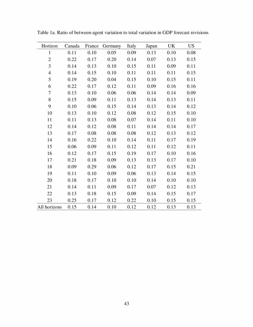
43

Table 1a. Ratio of between-agent variation to total variation in GDP forecast revisions

Horizon Canada France Germany Italy Japan UK US

1 0.11 0.10 0.05 0.09 0.13 0.10 0.08

2 0.22 0.17 0.20 0.14 0.07 0.13 0.15

3 0.14 0.13 0.10 0.15 0.11 0.09 0.11

4 0.14 0.15 0.10 0.11 0.11 0.11 0.15

5 0.19 0.20 0.04 0.15 0.10 0.15 0.11

6 0.22 0.17 0.12 0.11 0.09 0.16 0.16

7 0.13 0.10 0.06 0.06 0.14 0.14 0.09

8 0.15 0.09 0.11 0.13 0.14 0.13 0.11

9 0.10 0.06 0.15 0.14 0.13 0.14 0.12

10 0.13 0.10 0.12 0.08 0.12 0.15 0.10

11 0.11 0.13 0.08 0.07 0.14 0.11 0.10

12 0.14 0.12 0.08 0.11 0.14 0.14 0.17

13 0.17 0.08 0.08 0.08 0.12 0.13 0.12

14 0.16 0.22 0.10 0.14 0.11 0.17 0.19

15 0.06 0.09 0.11 0.12 0.11 0.12 0.11

16 0.12 0.17 0.15 0.19 0.17 0.10 0.16

17 0.21 0.18 0.09 0.13 0.13 0.17 0.10

18 0.09 0.29 0.06 0.12 0.17 0.15 0.21

19 0.11 0.10 0.09 0.06 0.13 0.14 0.15

20 0.18 0.17 0.10 0.10 0.14 0.10 0.10

21 0.14 0.11 0.09 0.17 0.07 0.12 0.13

22 0.13 0.18 0.15 0.09 0.14 0.15 0.17

23 0.25 0.17 0.12 0.22 0.10 0.15 0.15

All horizons 0.15 0.14 0.10 0.12 0.12 0.13 0.13

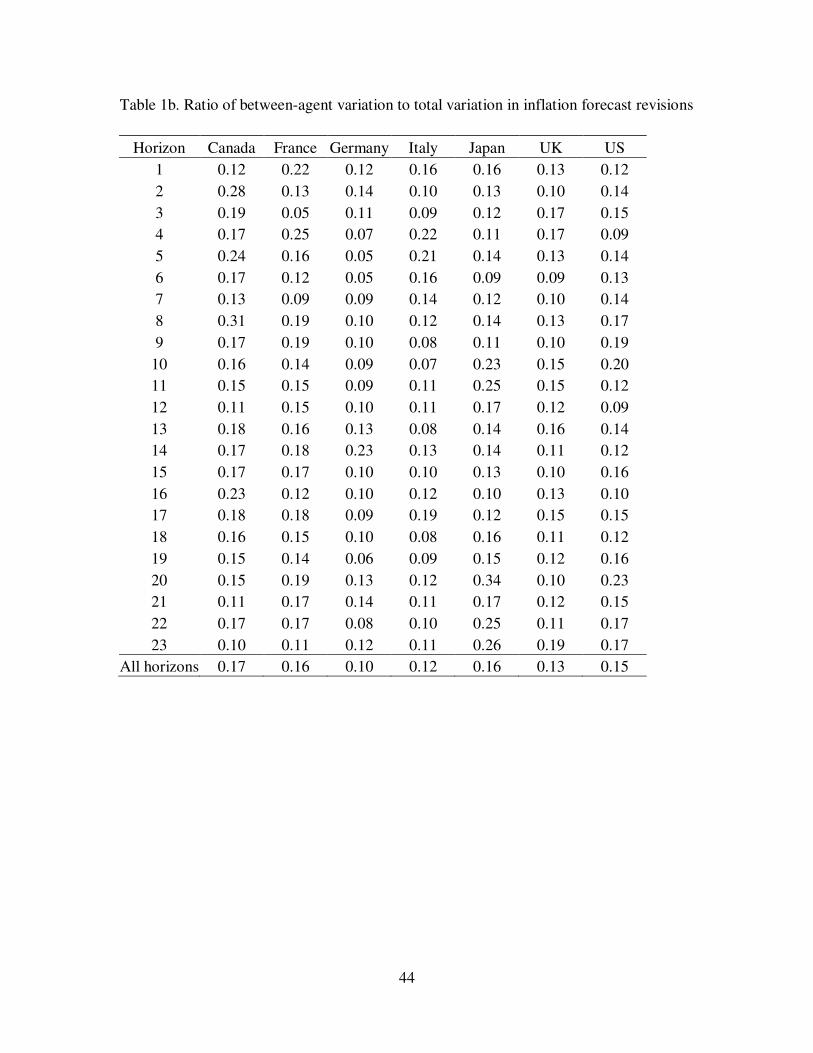
44

Table 1b. Ratio of between-agent variation to total variation in inflation forecast revisions

Horizon Canada France Germany Italy Japan UK US

1 0.12 0.22 0.12 0.16 0.16 0.13 0.12

2 0.28 0.13 0.14 0.10 0.13 0.10 0.14

3 0.19 0.05 0.11 0.09 0.12 0.17 0.15

4 0.17 0.25 0.07 0.22 0.11 0.17 0.09

5 0.24 0.16 0.05 0.21 0.14 0.13 0.14

6 0.17 0.12 0.05 0.16 0.09 0.09 0.13

7 0.13 0.09 0.09 0.14 0.12 0.10 0.14

8 0.31 0.19 0.10 0.12 0.14 0.13 0.17

9 0.17 0.19 0.10 0.08 0.11 0.10 0.19

10 0.16 0.14 0.09 0.07 0.23 0.15 0.20

11 0.15 0.15 0.09 0.11 0.25 0.15 0.12

12 0.11 0.15 0.10 0.11 0.17 0.12 0.09

13 0.18 0.16 0.13 0.08 0.14 0.16 0.14

14 0.17 0.18 0.23 0.13 0.14 0.11 0.12

15 0.17 0.17 0.10 0.10 0.13 0.10 0.16

16 0.23 0.12 0.10 0.12 0.10 0.13 0.10

17 0.18 0.18 0.09 0.19 0.12 0.15 0.15

18 0.16 0.15 0.10 0.08 0.16 0.11 0.12

19 0.15 0.14 0.06 0.09 0.15 0.12 0.16

20 0.15 0.19 0.13 0.12 0.34 0.10 0.23

21 0.11 0.17 0.14 0.11 0.17 0.12 0.15

22 0.17 0.17 0.08 0.10 0.25 0.11 0.17

23 0.10 0.11 0.12 0.11 0.26 0.19 0.17

All horizons 0.17 0.16 0.10 0.12 0.16 0.13 0.15

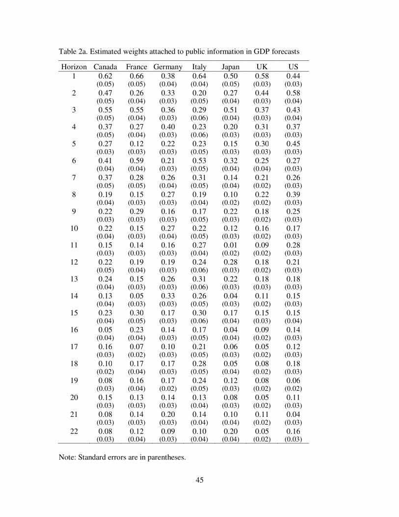
45

Table 2a. Estimated weights attached to public information in GDP forecasts

Horizon Canada France Germany Italy Japan UK US 1 0.62 0.66 0.38 0.64 0.50 0.58 0.44 (0.05) (0.05) (0.04) (0.04) (0.05) (0.03) (0.03)

2 0.47 0.26 0.33 0.20 0.27 0.44 0.58 (0.05) (0.04) (0.03) (0.05) (0.04) (0.03) (0.04)

3 0.55 0.55 0.36 0.29 0.51 0.37 0.43 (0.05) (0.04) (0.03) (0.06) (0.04) (0.03) (0.04)

4 0.37 0.27 0.40 0.23 0.20 0.31 0.37 (0.05) (0.04) (0.03) (0.06) (0.03) (0.03) (0.03)

5 0.27 0.12 0.22 0.23 0.15 0.30 0.45 (0.03) (0.03) (0.03) (0.05) (0.03) (0.03) (0.03)

6 0.41 0.59 0.21 0.53 0.32 0.25 0.27 (0.04) (0.04) (0.03) (0.05) (0.04) (0.04) (0.03)

7 0.37 0.28 0.26 0.31 0.14 0.21 0.26 (0.05) (0.05) (0.04) (0.05) (0.04) (0.02) (0.03)

8 0.19 0.15 0.27 0.19 0.10 0.22 0.39 (0.04) (0.03) (0.03) (0.04) (0.02) (0.02) (0.03)

9 0.22 0.29 0.16 0.17 0.22 0.18 0.25 (0.03) (0.03) (0.03) (0.05) (0.03) (0.02) (0.03)

10 0.22 0.15 0.27 0.22 0.12 0.16 0.17 (0.04) (0.03) (0.04) (0.05) (0.03) (0.02) (0.03)

11 0.15 0.14 0.16 0.27 0.01 0.09 0.28 (0.03) (0.03) (0.03) (0.04) (0.02) (0.02) (0.03)

12 0.22 0.19 0.19 0.24 0.28 0.18 0.21 (0.05) (0.04) (0.03) (0.06) (0.03) (0.02) (0.03)

13 0.24 0.15 0.26 0.31 0.22 0.18 0.18 (0.04) (0.03) (0.03) (0.06) (0.03) (0.03) (0.03)

14 0.13 0.05 0.33 0.26 0.04 0.11 0.15 (0.04) (0.03) (0.03) (0.05) (0.03) (0.02) (0.03)

15 0.23 0.30 0.17 0.30 0.17 0.15 0.15 (0.04) (0.05) (0.03) (0.06) (0.04) (0.03) (0.04)

16 0.05 0.23 0.14 0.17 0.04 0.09 0.14 (0.04) (0.04) (0.03) (0.05) (0.04) (0.02) (0.03)

17 0.16 0.07 0.10 0.21 0.06 0.05 0.12 (0.03) (0.02) (0.03) (0.05) (0.03) (0.02) (0.03)

18 0.10 0.17 0.17 0.28 0.05 0.08 0.18 (0.02) (0.04) (0.03) (0.05) (0.04) (0.02) (0.03)

19 0.08 0.16 0.17 0.24 0.12 0.08 0.06 (0.03) (0.04) (0.02) (0.05) (0.03) (0.02) (0.02)

20 0.15 0.13 0.14 0.13 0.08 0.05 0.11 (0.03) (0.03) (0.03) (0.04) (0.03) (0.02) (0.03)

21 0.08 0.14 0.20 0.14 0.10 0.11 0.04 (0.03) (0.03) (0.03) (0.04) (0.04) (0.02) (0.03)

22 0.08 0.12 0.09 0.10 0.20 0.05 0.16 (0.03) (0.04) (0.03) (0.04) (0.04) (0.02) (0.03)

Note: Standard errors are in parentheses.

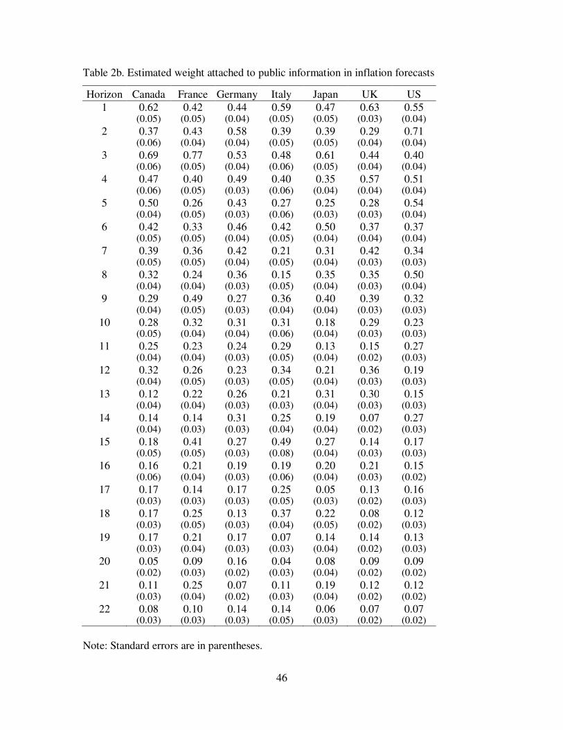
46

Table 2b. Estimated weight attached to public information in inflation forecasts

Horizon Canada France Germany Italy Japan UK US 1 0.62 0.42 0.44 0.59 0.47 0.63 0.55 (0.05) (0.05) (0.04) (0.05) (0.05) (0.03) (0.04)

2 0.37 0.43 0.58 0.39 0.39 0.29 0.71 (0.06) (0.04) (0.04) (0.05) (0.05) (0.04) (0.04)

3 0.69 0.77 0.53 0.48 0.61 0.44 0.40 (0.06) (0.05) (0.04) (0.06) (0.05) (0.04) (0.04)

4 0.47 0.40 0.49 0.40 0.35 0.57 0.51 (0.06) (0.05) (0.03) (0.06) (0.04) (0.04) (0.04)

5 0.50 0.26 0.43 0.27 0.25 0.28 0.54 (0.04) (0.05) (0.03) (0.06) (0.03) (0.03) (0.04)

6 0.42 0.33 0.46 0.42 0.50 0.37 0.37 (0.05) (0.05) (0.04) (0.05) (0.04) (0.04) (0.04)

7 0.39 0.36 0.42 0.21 0.31 0.42 0.34 (0.05) (0.05) (0.04) (0.05) (0.04) (0.03) (0.03)

8 0.32 0.24 0.36 0.15 0.35 0.35 0.50 (0.04) (0.04) (0.03) (0.05) (0.04) (0.03) (0.04)

9 0.29 0.49 0.27 0.36 0.40 0.39 0.32 (0.04) (0.05) (0.03) (0.04) (0.04) (0.03) (0.03)

10 0.28 0.32 0.31 0.31 0.18 0.29 0.23 (0.05) (0.04) (0.04) (0.06) (0.04) (0.03) (0.03)

11 0.25 0.23 0.24 0.29 0.13 0.15 0.27 (0.04) (0.04) (0.03) (0.05) (0.04) (0.02) (0.03)

12 0.32 0.26 0.23 0.34 0.21 0.36 0.19 (0.04) (0.05) (0.03) (0.05) (0.04) (0.03) (0.03)

13 0.12 0.22 0.26 0.21 0.31 0.30 0.15 (0.04) (0.04) (0.03) (0.03) (0.04) (0.03) (0.03)

14 0.14 0.14 0.31 0.25 0.19 0.07 0.27 (0.04) (0.03) (0.03) (0.04) (0.04) (0.02) (0.03)

15 0.18 0.41 0.27 0.49 0.27 0.14 0.17 (0.05) (0.05) (0.03) (0.08) (0.04) (0.03) (0.03)

16 0.16 0.21 0.19 0.19 0.20 0.21 0.15 (0.06) (0.04) (0.03) (0.06) (0.04) (0.03) (0.02)

17 0.17 0.14 0.17 0.25 0.05 0.13 0.16 (0.03) (0.03) (0.03) (0.05) (0.03) (0.02) (0.03)

18 0.17 0.25 0.13 0.37 0.22 0.08 0.12 (0.03) (0.05) (0.03) (0.04) (0.05) (0.02) (0.03)

19 0.17 0.21 0.17 0.07 0.14 0.14 0.13 (0.03) (0.04) (0.03) (0.03) (0.04) (0.02) (0.03)

20 0.05 0.09 0.16 0.04 0.08 0.09 0.09 (0.02) (0.03) (0.02) (0.03) (0.04) (0.02) (0.02)

21 0.11 0.25 0.07 0.11 0.19 0.12 0.12 (0.03) (0.04) (0.02) (0.03) (0.04) (0.02) (0.02)

22 0.08 0.10 0.14 0.14 0.06 0.07 0.07 (0.03) (0.03) (0.03) (0.05) (0.03) (0.02) (0.02)

Note: Standard errors are in parentheses.

47

Table 3a. Test of efficiency in the use of public information in GDP forecasts

Horizon Canada France Germany Italy Japan UK US 1 -0.17 0.01 0.11 -0.10 0.21* -0.18* 0.61* (-1.37) (0.11) (0.76) (-1.04) (2.29) (-2.09) (3.61)

2 0.67* 0.39 1.03* 0.02 -0.23 -0.33* -0.30* (3.44) (1.72) (5.01) (0.14) (-1.25) (-3.08) (-2.41)

3 0.14 0.19 0.63* 0.28* 0.02 -0.14 -0.16 (1.27) (1.46) (3.33) (2.62) (0.25) (-1.62) (-1.37)

4 0.29* 0.09 0.72* 0.41* 0.10 0.16 -0.14 (2.38) (0.57) (6.03) (2.20) (0.86) (1.83) (-1.07)

5 0.13 0.18 1.00* 0.48 -0.18 0.24* -0.30* (0.54) (0.53) (5.61) (1.80) (-0.82) (2.68) (-2.72)

6 0.00 0.10 1.16* 0.08 0.06 0.10 -0.13 (0.02) (0.77) (6.15) (0.64) (0.62) (1.16) (-0.86)

7 0.47* 0.30* 0.38* -0.01 -0.25 0.96* 0.34* (4.12) (2.29) (2.59) (-0.09) (-1.45) (5.79) (2.56)

8 0.68* 1.06* 0.43* 0.26 0.41 0.48* 0.21* (2.63) (4.38) (2.28) (1.07) (1.06) (3.12) (2.27)

9 0.60* 0.87* 0.32 0.03 0.77* 0.49* 0.27* (3.03) (5.12) (1.23) (0.12) (4.27) (3.24) (2.04)

10 1.01* 1.38* 0.09 0.16 -0.15 0.40* 0.09 (5.27) (6.59) (0.52) (0.69) (-0.66) (2.20) (0.70)

11 1.74* 1.25* 0.82* 0.62* 0.18 1.12* 0.50* (6.01) (4.03) (3.63) (2.53) (0.45) (5.43) (5.23)

12 0.89* 0.84* 0.95* 0.29 0.23 0.85* 0.45* (3.74) (3.22) (4.56) (1.20) (1.19) (5.22) (2.82)

13 0.78* 0.74* 0.84* 0.34 0.01 0.09 0.96* (2.33) (2.76) (4.49) (1.36) (0.03) (0.51) (4.99)

14 -0.23 1.05* 0.99* 0.56* 0.10 -0.12 0.25 (-0.56) (2.85) (4.81) (2.08) (0.34) (-0.61) (1.29)

15 -0.68* 0.37 1.21* 0.63* -0.09 0.51* -0.39* (-2.64) (1.78) (5.02) (2.94) (-0.44) (2.82) (-2.63)

16 -0.90* 0.72* 0.92* 0.01 0.12 0.38 0.59* (-2.42) (2.14) (2.85) (0.02) (0.49) (1.55) (3.31)

17 0.48 1.92* 1.03* 1.25* 0.15 -0.38 0.06 (0.98) (2.45) (2.92) (2.44) (0.33) (-1.52) (0.23)

18 1.02 -0.98* 0.03 -0.13 0.14 0.19 0.70* (1.75) (-2.78) (0.09) (-0.38) (0.43) (0.74) (2.19)

19 -0.80 -2.07* -0.15 -0.22 -0.74 -0.11 0.73 (-1.92) (-6.42) (-0.38) (-0.57) (-1.65) (-0.36) (1.81)

20 1.56* -1.23* -0.47 -0.46 -0.99 0.00 -0.02 (3.25) (-2.11) (-1.16) (-0.89) (-1.76) (0.01) (-0.06)

21 0.08 0.61 0.51 0.40 -0.18 0.20 -0.13 (0.17) (1.12) (1.47) (0.72) (-0.40) (0.63) (-0.39)

22 -0.28 -0.78 0.01 -1.73* 0.89* -0.01 -0.52 (-0.49) (-1.73) (0.04) (-3.43) (2.07) (-0.01) (-1.49)

23 -0.69 -0.29 -0.27 -0.70 0.28 -0.39 -0.73* (-1.65) (-0.49) (-0.69) (-1.34) (0.42) (-1.12) (-2.57)

Note: t-statistics are shown in parentheses. A single * denotes that the estimated values are statistically significant at the 5% level.

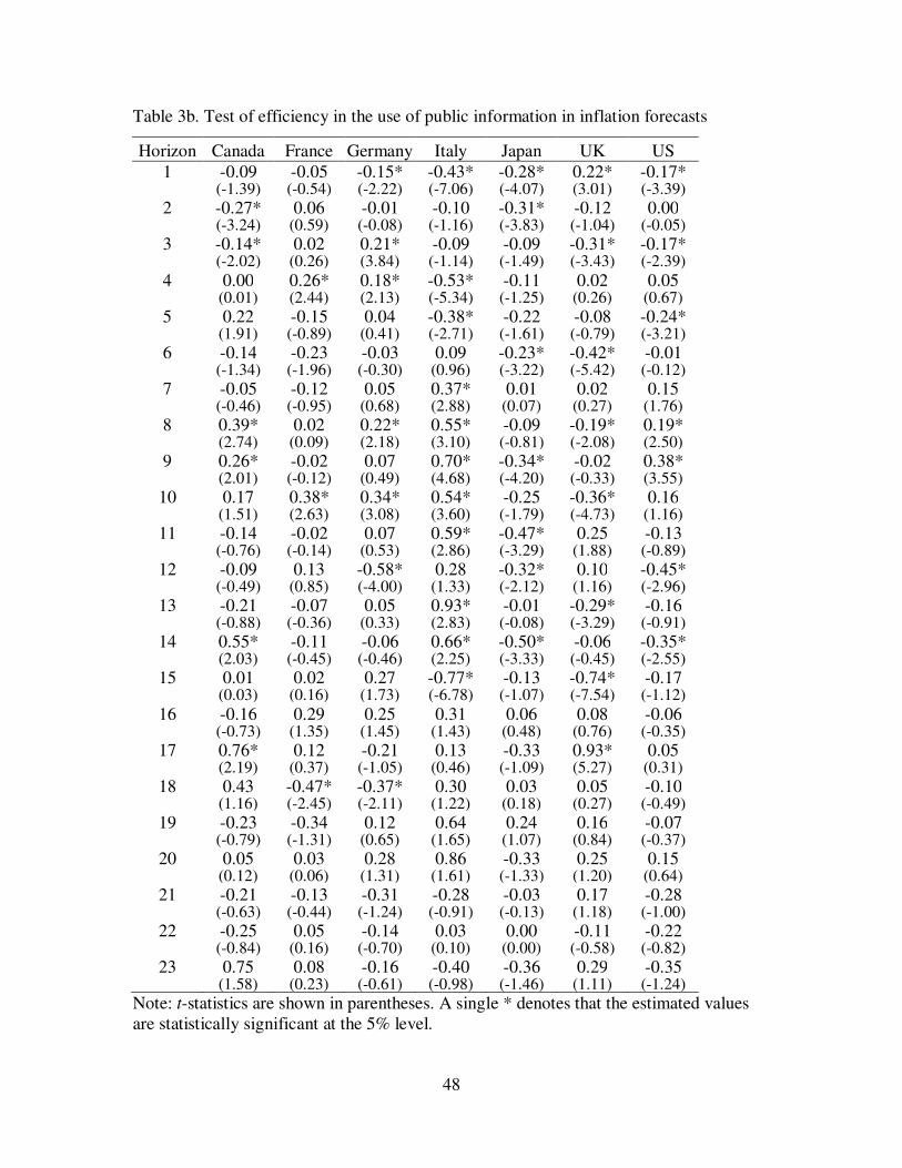
48

Table 3b. Test of efficiency in the use of public information in inflation forecasts

Horizon Canada France Germany Italy Japan UK US 1 -0.09 -0.05 -0.15* -0.43* -0.28* 0.22* -0.17* (-1.39) (-0.54) (-2.22) (-7.06) (-4.07) (3.01) (-3.39)

2 -0.27* 0.06 -0.01 -0.10 -0.31* -0.12 0.00 (-3.24) (0.59) (-0.08) (-1.16) (-3.83) (-1.04) (-0.05)

3 -0.14* 0.02 0.21* -0.09 -0.09 -0.31* -0.17* (-2.02) (0.26) (3.84) (-1.14) (-1.49) (-3.43) (-2.39)

4 0.00 0.26* 0.18* -0.53* -0.11 0.02 0.05 (0.01) (2.44) (2.13) (-5.34) (-1.25) (0.26) (0.67)

5 0.22 -0.15 0.04 -0.38* -0.22 -0.08 -0.24* (1.91) (-0.89) (0.41) (-2.71) (-1.61) (-0.79) (-3.21)

6 -0.14 -0.23 -0.03 0.09 -0.23* -0.42* -0.01 (-1.34) (-1.96) (-0.30) (0.96) (-3.22) (-5.42) (-0.12)

7 -0.05 -0.12 0.05 0.37* 0.01 0.02 0.15 (-0.46) (-0.95) (0.68) (2.88) (0.07) (0.27) (1.76)

8 0.39* 0.02 0.22* 0.55* -0.09 -0.19* 0.19* (2.74) (0.09) (2.18) (3.10) (-0.81) (-2.08) (2.50)

9 0.26* -0.02 0.07 0.70* -0.34* -0.02 0.38* (2.01) (-0.12) (0.49) (4.68) (-4.20) (-0.33) (3.55)

10 0.17 0.38* 0.34* 0.54* -0.25 -0.36* 0.16 (1.51) (2.63) (3.08) (3.60) (-1.79) (-4.73) (1.16)

11 -0.14 -0.02 0.07 0.59* -0.47* 0.25 -0.13 (-0.76) (-0.14) (0.53) (2.86) (-3.29) (1.88) (-0.89)

12 -0.09 0.13 -0.58* 0.28 -0.32* 0.10 -0.45* (-0.49) (0.85) (-4.00) (1.33) (-2.12) (1.16) (-2.96)

13 -0.21 -0.07 0.05 0.93* -0.01 -0.29* -0.16 (-0.88) (-0.36) (0.33) (2.83) (-0.08) (-3.29) (-0.91)

14 0.55* -0.11 -0.06 0.66* -0.50* -0.06 -0.35* (2.03) (-0.45) (-0.46) (2.25) (-3.33) (-0.45) (-2.55)

15 0.01 0.02 0.27 -0.77* -0.13 -0.74* -0.17 (0.03) (0.16) (1.73) (-6.78) (-1.07) (-7.54) (-1.12)

16 -0.16 0.29 0.25 0.31 0.06 0.08 -0.06 (-0.73) (1.35) (1.45) (1.43) (0.48) (0.76) (-0.35)

17 0.76* 0.12 -0.21 0.13 -0.33 0.93* 0.05 (2.19) (0.37) (-1.05) (0.46) (-1.09) (5.27) (0.31)

18 0.43 -0.47* -0.37* 0.30 0.03 0.05 -0.10 (1.16) (-2.45) (-2.11) (1.22) (0.18) (0.27) (-0.49)

19 -0.23 -0.34 0.12 0.64 0.24 0.16 -0.07 (-0.79) (-1.31) (0.65) (1.65) (1.07) (0.84) (-0.37)

20 0.05 0.03 0.28 0.86 -0.33 0.25 0.15 (0.12) (0.06) (1.31) (1.61) (-1.33) (1.20) (0.64)

21 -0.21 -0.13 -0.31 -0.28 -0.03 0.17 -0.28 (-0.63) (-0.44) (-1.24) (-0.91) (-0.13) (1.18) (-1.00)

22 -0.25 0.05 -0.14 0.03 0.00 -0.11 -0.22 (-0.84) (0.16) (-0.70) (0.10) (0.00) (-0.58) (-0.82)

23 0.75 0.08 -0.16 -0.40 -0.36 0.29 -0.35 (1.58) (0.23) (-0.61) (-0.98) (-1.46) (1.11) (-1.24)

Note: t-statistics are shown in parentheses. A single * denotes that the estimated values are statistically significant at the 5% level.

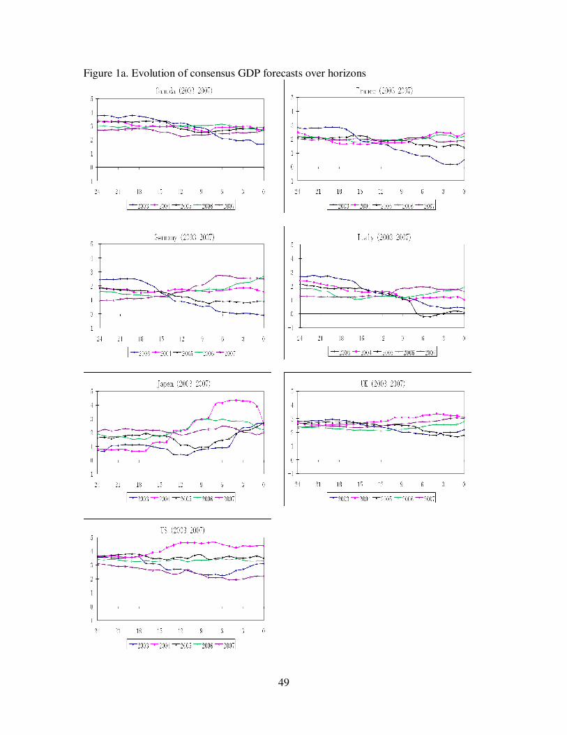
49

Figure 1a. Evolution of consensus GDP forecasts over horizons

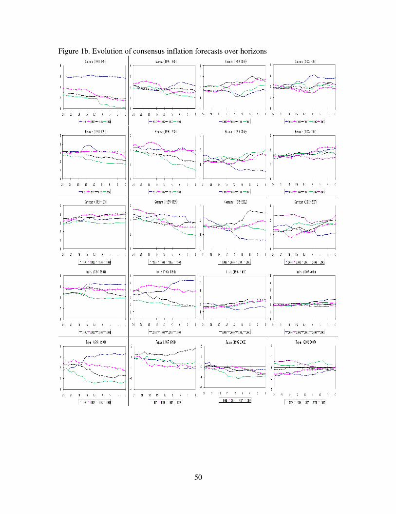
50

Figure 1b. Evolution of consensus inflation forecasts over horizons

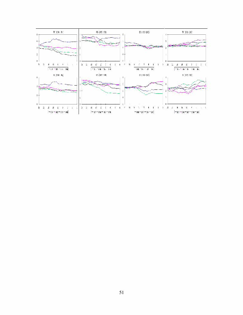
51

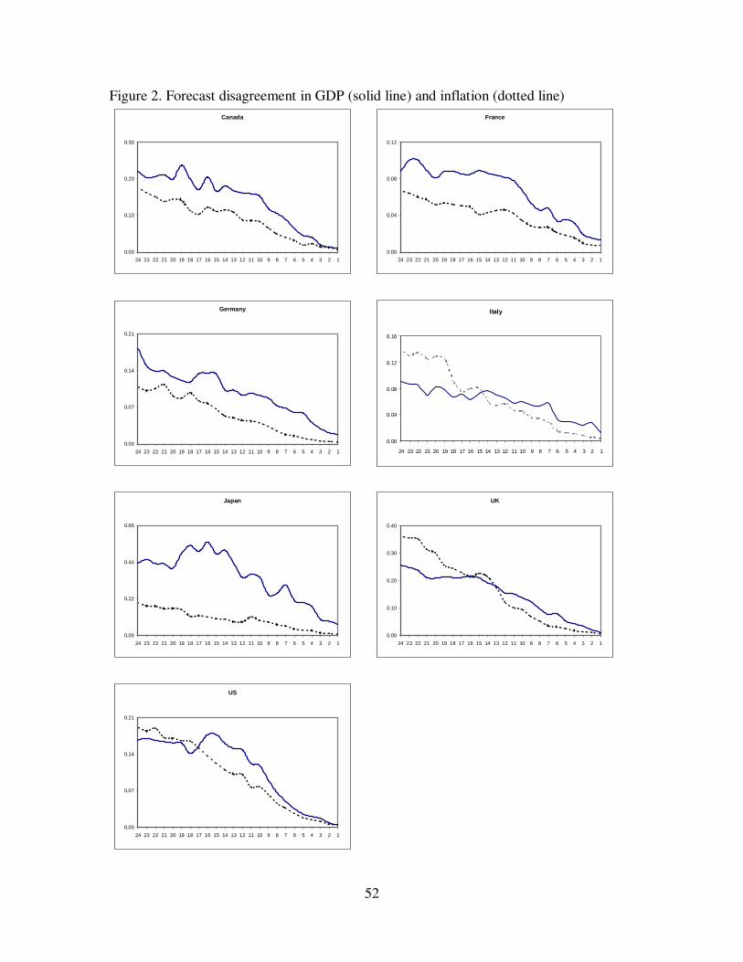
52

Figure 2. Forecast disagreement in GDP (solid line) and inflation (dotted line) Canada

0.00

0.10

0.20

0.30

123456789101112131415161718192021222324

France

0.00

0.04

0.08

0.12

123456789101112131415161718192021222324

Germany

0.00

0.07

0.14

0.21

123456789101112131415161718192021222324

Italy

0.00

0.04

0.08

0.12

0.16

123456789101112131415161718192021222324

Japan

0.00

0.22

0.44

0.66

123456789101112131415161718192021222324

UK

0.00

0.10

0.20

0.30

0.40

123456789101112131415161718192021222324

US

0.00

0.07

0.14

0.21

123456789101112131415161718192021222324

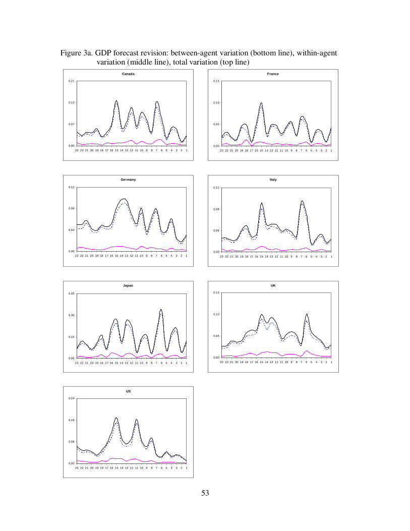
53

Figure 3a. GDP forecast revision: between-agent variation (bottom line), within-agent variation (middle line), total variation (top line)

Canada

0.00

0.07

0.14

0.21

1234567891011121314151617181920212223

France

0.00

0.05

0.10

0.15

1234567891011121314151617181920212223

Germany

0.00

0.04

0.08

0.12

1234567891011121314151617181920212223

Italy

0.00

0.04

0.08

0.12

1234567891011121314151617181920212223

Japan

0.00

0.15

0.30

0.45

1234567891011121314151617181920212223

UK

0.00

0.05

0.10

0.15

1234567891011121314151617181920212223

US

0.00

0.08

0.16

0.24

1234567891011121314151617181920212223

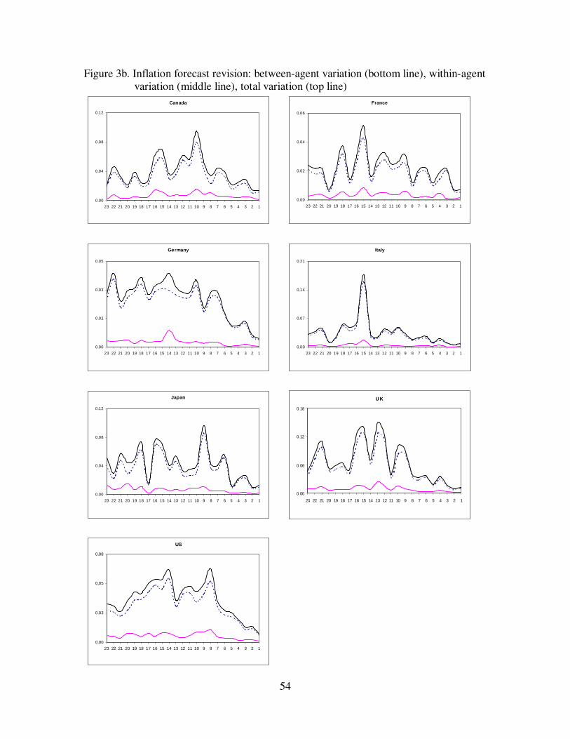
54

Figure 3b. Inflation forecast revision: between-agent variation (bottom line), within-agent variation (middle line), total variation (top line)

Canada

0.00

0.04

0.08

0.12

1234567891011121314151617181920212223

France

0.00

0.02

0.04

0.06

1234567891011121314151617181920212223

Germany

0.00

0.02

0.03

0.05

1234567891011121314151617181920212223

Italy

0.00

0.07

0.14

0.21

1234567891011121314151617181920212223

Japan

0.00

0.04

0.08

0.12

1234567891011121314151617181920212223

U K

0.00

0.06

0.12

0.18

1234567891011121314151617181920212223

US

0.00

0.03

0.05

0.08

1234567891011121314151617181920212223

55

Figure 4. RMSEs in real GDP (solid line) and inflation forecasts (dotted line)

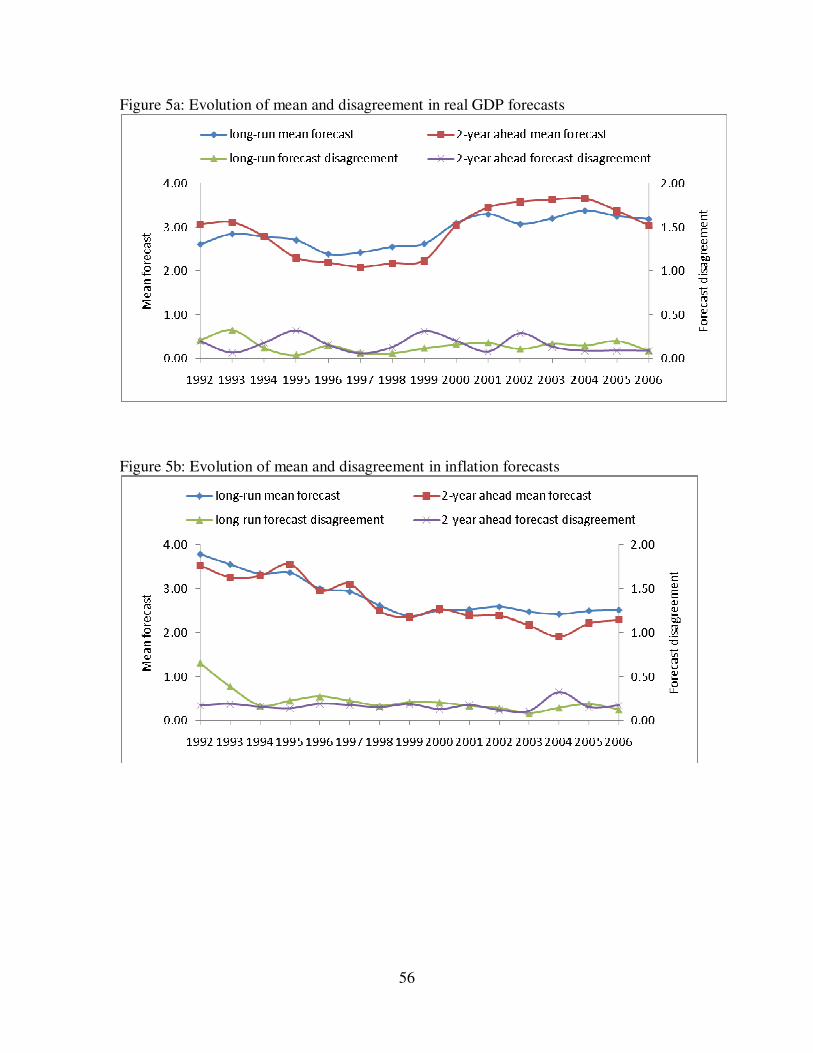
56

Figure 5a: Evolution of mean and disagreement in real GDP forecasts

Figure 5b: Evolution of mean and disagreement in inflation forecasts

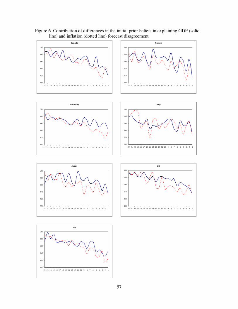
57

Figure 6. Contribution of differences in the initial prior beliefs in explaining GDP (solid line) and inflation (dotted line) forecast disagreement

Canada

0.00

0.20

0.40

0.60

0.80

1.00

12345678910111213141516171819202122

France

0.00

0.20

0.40

0.60

0.80

1.00

12345678910111213141516171819202122

Germany

0.00

0.20

0.40

0.60

0.80

1.00

12345678910111213141516171819202122

Italy

0.00

0.20

0.40

0.60

0.80

1.00

12345678910111213141516171819202122

Japan

0.00

0.20

0.40

0.60

0.80

1.00

12345678910111213141516171819202122

UK

0.00

0.20

0.40

0.60

0.80

1.00

12345678910111213141516171819202122

US

0.00

0.20

0.40

0.60

0.80

1.00

12345678910111213141516171819202122

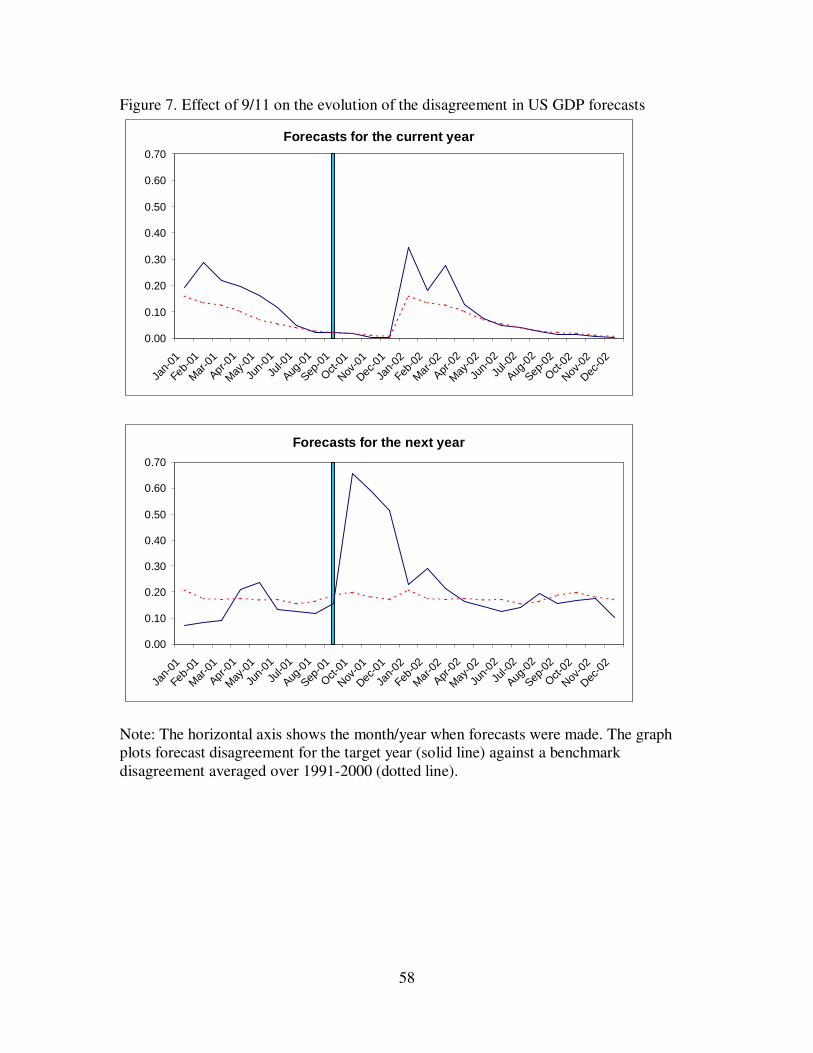
58

Figure 7. Effect of 9/11 on the evolution of the disagreement in US GDP forecasts

Forecasts for the current year

0.00

0.10

0.20

0.30

0.40

0.50

0.60

0.70

Jan-

01

Feb-

01

Mar

-01

Apr-0

1

May

-01

Jun-

01

Jul-0

1

Aug-0

1

Sep-0

1

Oct-01

Nov-0

1

Dec-0

1

Jan-

02

Feb-0

2

Mar

-02

Apr-0

2

May

-02

Jun-

02

Jul-0

2

Aug-0

2

Sep-0

2

Oct-02

Nov-0

2

Dec-0

2

Forecasts for the next year

0.00

0.10

0.20

0.30

0.40

0.50

0.60

0.70

Jan-

01

Feb-

01

Mar

-01

Apr-0

1

May

-01

Jun-

01

Jul-0

1

Aug-0

1

Sep-0

1

Oct-01

Nov-0

1

Dec-0

1

Jan-

02

Feb-0

2

Mar

-02

Apr-0

2

May

-02

Jun-

02

Jul-0

2

Aug-0

2

Sep-0

2

Oct-02

Nov-0

2

Dec-0

2

Note: The horizontal axis shows the month/year when forecasts were made. The graph plots forecast disagreement for the target year (solid line) against a benchmark disagreement averaged over 1991-2000 (dotted line).

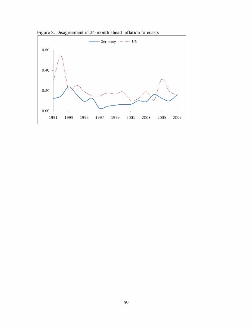
59

Figure 8. Disagreement in 24-month ahead inflation forecasts

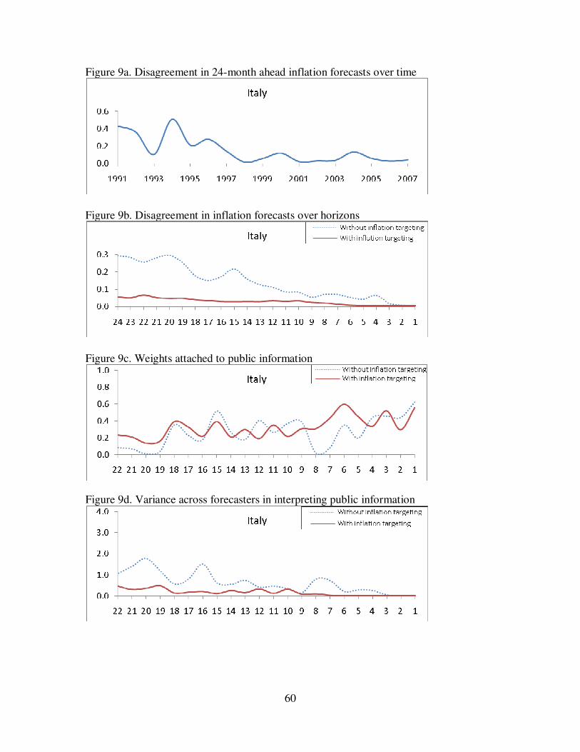
60

Figure 9a. Disagreement in 24-month ahead inflation forecasts over time

Figure 9b. Disagreement in inflation forecasts over horizons

Figure 9c. Weights attached to public information

Figure 9d. Variance across forecasters in interpreting public information

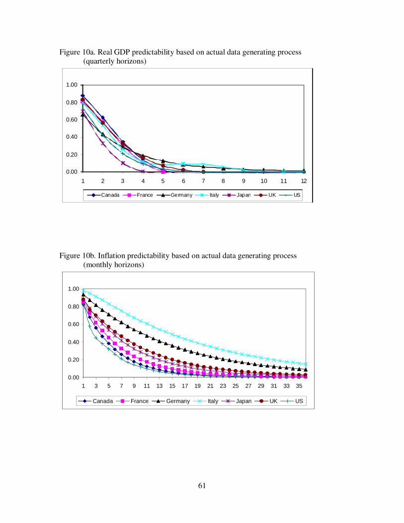
61

Figure 10a. Real GDP predictability based on actual data generating process (quarterly horizons)

0.00

0.20

0.40

0.60

0.80

1.00

1 2 3 4 5 6 7 8 9 10 11 12

Canada France Germany Italy Japan UK US

Figure 10b. Inflation predictability based on actual data generating process

(monthly horizons)

0.00

0.20

0.40

0.60

0.80

1.00

1 3 5 7 9 11 13 15 17 19 21 23 25 27 29 31 33 35

Canada France Germany Italy Japan UK US

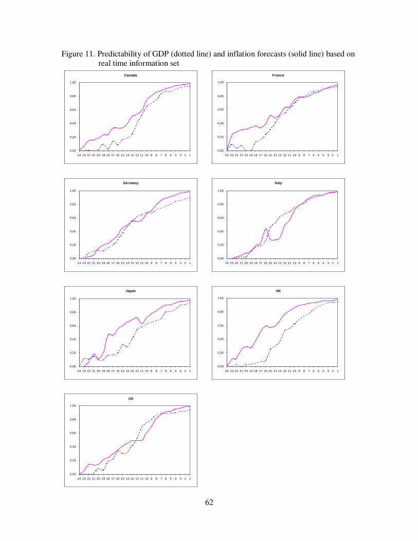
62

Figure 11. Predictability of GDP (dotted line) and inflation forecasts (solid line) based on real time information set

Canada

0.00

0.20

0.40

0.60

0.80

1.00

123456789101112131415161718192021222324

France

0.00

0.20

0.40

0.60

0.80

1.00

123456789101112131415161718192021222324

Germany

0.00

0.20

0.40

0.60

0.80

1.00

123456789101112131415161718192021222324

Italy

0.00

0.20

0.40

0.60

0.80

1.00

123456789101112131415161718192021222324

Japan

0.00

0.20

0.40

0.60

0.80

1.00

123456789101112131415161718192021222324

UK

0.00

0.20

0.40

0.60

0.80

1.00

123456789101112131415161718192021222324

US

0.00

0.20

0.40

0.60

0.80

1.00

123456789101112131415161718192021222324