Kupy galaxií – lekce IIIKupy galaxií – lekce III

Pavel Jáchym

OverviewOverview

Numerical simulations◦N-body◦tree method◦sticky particles◦SPH vs. grid codes◦genetic algorithms

Applications: ram pressure strippingICM - recapitulationCluster mass from gravitational lensing

Environmental effectsEnvironmental effects

Morphological evolution: more spirals at z=0.5 than at z=0 (Dressler 1980)

Morphology-density relationFraction of blue galaxies increases with z (Butcher &

Oemler effect, 1978)HI deficiency (Davies & Lewis 1973)Dynamical perturbations (Rubin et al. 1999)...

Interaction of spirals with environmentInteraction of spirals with environment

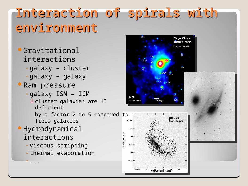
Gravitational interactions◦galaxy – cluster◦galaxy – galaxy

Ram pressure◦galaxy ISM – ICM

cluster galaxies are HI deficient by a factor 2 to 5 compared to field galaxies

Hydrodynamical interactions◦ viscous stripping◦ thermal evaporation◦ ...

Galaxy mergersGalaxy mergers In the hierarchical CDM model, present-day galaxies are built up in

a sequence of mergers from originally small objects similar to irregulars

The outcome of a merger between two galaxies depends on the mass-ratio between the two objects, their intrinsic and orbital angular momenta and their gas content◦ mass-ratio < 1:4 does not change much the structure of the more massive

galaxy◦ mergers between two late-type spirals may create an S0 or an elliptical ◦ mergers between an elliptical and a spiral could produce an elliptical or an S0

galaxy◦ generally: merger between two galaxies produces a remnant of an earlier type

in the Hubble diagram◦ the orbital angular momentum of the galaxies is absorbed into the angular momentum

of the remnant’s halo◦ the gas quickly moves to the center of the merger remnant; it may feed nuclear BHs◦ ULIRGs show the final stages of spiral-spiral merger with heavy star-formation taking

place

Evolution of spiralsEvolution of spirals Possible scenario for spirals transforming into S0’s

◦ infalling spiral galaxies at z=0.5◦ triggering star formation◦ starburst (emission-line galaxies)◦ gas stripping by intracluster medium◦ post-starburst galaxies◦ tidal interactions heat disk◦ stars fade◦ S0 galaxies at z=0

morphological segregation proceeds hierarchically, affecting richer and denser groups earlier. S0’s are only formed after cluster virialization.

A note to the formation of clustersA note to the formation of clusters

Chandra survey of the Fornax galaxy cluster revealed a vast, swept-back cloud of hot gas near the center of the cluster◦ the hot gas cloud is moving rapidly

through a larger, less dense cloud of gas

Shock fronts and cold frontsShock fronts and cold fronts

typical relative velocity for merging clusters is ~2000 km/s

a cold clump of gas is moving through a warmer medium

A sequence …A sequence …

Clusters

Groups

Ellipticals

sol15

8

10~

K10~

MM

T

sol13

7

10~

K10~

MM

T

sol12

7

10~

K10~

MM

T

Numerical simulationsNumerical simulationsGravitational interactions

◦ test particles◦direct summation◦ tree codes◦…

Hydrodynamical interactions ◦SPH◦finite difference codes

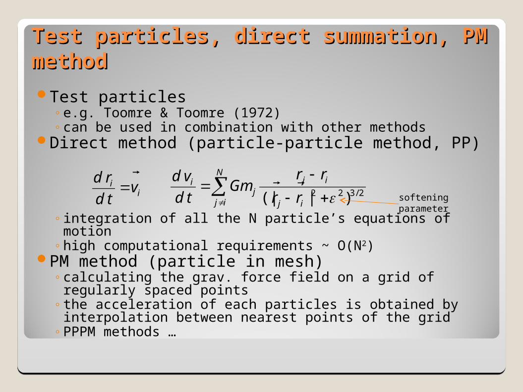
Test particles, direct summation, PM methodTest particles, direct summation, PM methodTest particles

◦ e.g. Toomre & Toomre (1972) ◦ can be used in combination with other methods

Direct method (particle-particle method, PP)

◦ integration of all the N particle’s equations of motion◦ high computational requirements ~ O(N2)

PM method (particle in mesh)◦ calculating the grav. force field on a grid of regularly spaced points◦ the acceleration of each particles is obtained by interpolation

between nearest points of the grid◦ PPPM methods …

ii vtd

rd

N

ij ij

ijj

i

rr

rrGm

td

vd2/322 )|(|

softeningparameter

Tree algorithmTree algorithm Lagrangian technique Uses direct summation to compute attraction

of close particles Detailed internal structure of distant groups

of particles may be ignored many similar particle – distant-particle interactions

are replaced with a single particle-group interaction Particles are organized into a hierarchic

structure of groups and cells resembling a tree ◦ - e.g. oct-tree scheme (see Fig.)◦ alternative AJP method

The influence of remote particles is obtained by evaluating the multipole expansion of the group

computational cost scales as O(N logN)

Tree algorithm, cont.Tree algorithm, cont. once the tree is completed, information about masses, center-of-

mass positions, and multipole moments are appended to each cell

the multipole expansion of a cell is used only if "opening" criterion is fulfilled: d > l / θ◦ d … distance of the cell◦ l … size of the cell◦ θ … opening angle

the opening criterion follows from comparison of the size of the quadrupole term with the size of the monopole term◦ higher-order multipoles of the gravitational field decay rapidly with respect to

the dominant monopole term◦ it is possible to approximate the group's potential only by monopole term, or

low-order corrections for the group's internal structure can be included as well multipole expansion of the potential:

52

1)(

rr

MGr

rQr k

ijkjkkkij rxxmQ )3( 2,

Hydrodynamical calculationsHydrodynamical calculations Gasdynamics:

◦ continuity equation

◦ Euler equation

◦ energy equation

◦ + eq. of state

0 vdt

d

P

dt

dv

),(uX

vP

dt

du

uP )1(

SPH - methodologySPH - methodology Smoothed Particle Hydrodynamics

Lagrangian technique

an arbitrary physical field A(r) is interpolated as

◦ smoothing kernel function W(r;h) specifies the extent of the interpolation volume, it has a sharp peak about r=0 and satisfies two conditions:

in numerical implementation values of A(r) are known only at locations of a selected finite number of particles distributed with number density

then

number of neighboring particles N is fixed during the calculation

');'()'()( drhrrWrArA

1');'( drhrrW )'();'(lim0

rrhrrWh

j

jrrrn )()(

N

jj

j

jj hrrWrA

mrA1

);()(

)(

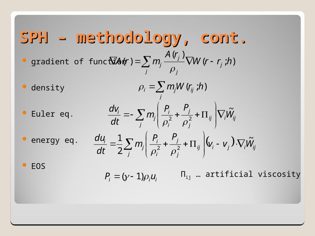
SPH – methodology, cont.SPH – methodology, cont. gradient of function

density

Euler eq.

energy eq.

EOS

j

jj

jj hrrWrA

mrA );()(

)(

j

ijji hrWm );(

jijiij

j

j

i

ij

i WPP

mdt

dv ~22

jijijiij

j

j

i

ij

i WvvPP

mdt

du ~

2

122

iii uP )1( Πij … artificial viscosity

Finite-difference methodFinite-difference method Eulerian technique approximates the solutions to differential equations using finite

difference equations to approximate derivatives grid-based codes for non-homogeneous systems – adaptive mesh refinement

hydrodynamics codes Ram pressure stripping simulation:

Roediger & Brüggen (2007)

ICM – recapitulationICM – recapitulation Intra-cluster medium

◦ optically thin plasma◦ thermal bremsstrahlung = braking radiation, free-free radiation◦ radiation by an unbound particle (e-) due to acceleration by

another charged particle (ion) Diffuse emission from a hot ICM is the direct manifestation of the

existence of a potential-well within which the gas is in dynamical equilibrium with the cool baryonic matter (galaxies) and the DM

X-ray luminosity is well correlated with the cluster mass and the X-ray emissivity is proportional to the square of the gas density

cluster emission is thus more concentrated than the optical bi-dimensional galaxy distribution

X-ray observationsX-ray observations X-rays are absorbed by the Earth’s atmosphere HEAO-1 X-ray Observatory was the first to provide a flux–limited

sample of X–ray identified clusters XMM-Newton & Chandra

◦ we can map the gas distribution in nearby clusters from very deep inside the core, at the scale of a few kpc with Chandra, up to very close to the virial radius with XMM-Newton

We can measure basic cluster properties up to high z~1.3◦ morphology from images, ◦ gas density radial profile, ◦ global temperature and gas mass ◦ total mass and entropy can be derived assuming isothermality

X-ray luminosities LX~1043 – 1045 erg/s◦ clusters are identifiable at large cosmological distances

X-ray surveysX-ray surveysFrom surveys several global observables can be derived:

◦ X-ray flux (luminosity if z known)◦ temperature

using scaling relations, these can be related to physical parameters, like mass, …

Scaling propertiesScaling propertiesbaryonic matter follows the DM grav. potential well it is heated by adiabatic compression during the halo mass

growth and by shocks induced by supersonic accretion or merger events

gravity dominates the process of gas heatingwhen assuming that the gas is in hydrostatic eq. with DM and

bremsstrahlung dominates the emissivity=>

however, from observations:◦ the luminosity-temperature relation is steeper (α=2.5-3 or even more in

groups)◦ also the relation between the gas mass and T is steeper (α=1.7-2)◦ this indicates that non-gravitational processes (SN, AGN feedbacks,

radiative cooling, winds, etc.) take place during the cluster formation and left an imprint on its X-ray properties

2/3virgas

2X , TMMTL

ICMICM typical cluster spectrum

◦ continuum emission dominated by thermal bremsst.

◦ main contribution from H and He◦ emissivity of the continuum

sensitive to temperature for energies > kT rather insensitive for energies lower

◦ iron K-line complex at 6.7 eV◦ intensity of other lines decreases with

increasing T shape of the spectrum determines T its normalisation then density ICM is not strictly isothermal – T from an

isothermal fit is a „mean“ value metallicity evolution:

Cooling of ICMCooling of ICMcooling timescale

◦ cooling function Λc(T)◦ tcool = kT / nΛc(T) > 1010 yr (n/10-3 cm-3)-1 (T/108 K)1/2

◦ in central cluster regions it can be shorter than the age of the Universe◦ in fairly relaxed clusters, the decrease of the ICM temp. in the central

regions has been recognized◦ cooling flows◦ supernovae or AGNs as possible feedback mechanisms providing an

adequate amount of extra energy to balance overcoolingthree ways how an electron can get rid of energy

◦ collisional cooling – very efficient but not for completely ionized ICM◦ Recombination – probability ~ 1/velocity => unimportant for ICM◦ free-free interaction = thermal bremsstrahlung

Cooling, cont.Cooling, cont. about 1000 Msol/yr of gas can cool out of the X-Ray halo this gas could form stars – some cD galaxies show filaments of gas

emission and blue colors in the central region others do not show the lower central temperatures that would be

expected if cooling was efficient presumably, cooling will lead to enhanced accretion of gas onto the black

hole in the cD galaxy ◦ it in turn may become active and provide high energy particles to heat the gas◦ thus, a quasi equilibrium may be established that prevents the gas from ever

forming stars still under debate …

Cooling, cont.Cooling, cont. Mixing via turbulence could counteract

cooling towards the outside Central AGNs can produce relativistic jets

which directly inject energy into the ICM and may cause shocks. Jets also inflate bubbles, which rise buoyantly, pushing colder gas upwards out of the core.

Acoustic waves produced by AGN outbursts can also transfer energy to the ICM if it is viscous enough

Characteristic time-scalesCharacteristic time-scales Mean free path for the ions and electrons of the ICM

◦ is << cluster size◦ ICM can be described by fluid dynamics …

Timescale for pressure equilibrium◦ if a region of gas undergoes a compression, how long does it take for

the pressure wave to propagate across the cluster?

◦ this is short compared to Hubble time – we can assume that the gas is in pressure eq.

33

ICM

28ICM

fp 10/

10/kpc 23

cmn

KT

2/1

H

2/1

s

m

kTPc

Mpc10yr 10 5.6/

2/1

88

sp

DTcDt

Characteristic time-scales, cont.Characteristic time-scales, cont. Timescale for cooling

◦ due to thermal emission◦ longer than a Hubble time◦ => hot gas stays hot!

Crossing time

Relaxation time◦ time-change to equil.

1

3-3-e

2/1

810

cool cm1010yr 10 2.2

nTt

1-

cl

9

clcross kms /1000

Mpc/yr 10~

DD

t

3-3-

2/388

relax cm /10

K10/yr 10 6n

Tt

Cluster mass estimatesCluster mass estimatesFrom the virial theoremFrom X-ray data

◦hydrostatic equilibrium condition

μ ... mean molecular weight (~0.59 for primordial composition)◦distribution of ICM

β ... ratio between the kinetic energy of any tracer of the grav. potential and the thermal energy of the gas

From gravitational lensing

rd

Td

rd

dr

mG

TkrM

ln

ln

ln

ln

)( gas

p

B

2/32c

0gas

/1)(

rr

r

Mass estimate from gravitational lensingMass estimate from gravitational lensing clusters act as grav. lenses on more distant galaxies one of the most important methods for the mass

determination of galaxy clusters the only method working for non-equilibrium systems! There are two rather different regimes

◦ Strong lensing background galaxies are strongly distorted good for massive clusters

◦ Weak lensing background galaxies only slightly distorted For a symmetric potential, the galaxies are elongated slightly in the

axial direction This is a "shearing" effect and only reveals the gradient in the

potential, not its integrated depth By measuring thousands of faint galaxy images, the effect is identified

statistically. shape and radial trend of the weak shear and strong lensing

effects yield the cluster mass distribution independent of the nature of the mass and therefore allow reliable total mass estimates including the dark matter

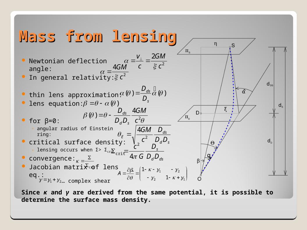
Mass from lensingMass from lensing Newtonian deflection angle: In general relativity:

thin lens approximation: lens equation:

for β=0: ◦ angular radius of Einstein ring:

critical surface density:◦ lensing occurs when Σ> Σcrit

convergence: Jacobian matrix of lens eq.:

2

2

c

GM

c

v

2

4

c

GM

)()(

s

ds

D

D ˆ

α

)(

2

4)(

c

GM

DD

D

sd

ds

sd

dsE DD

D

c

GM2

4

dsd

s

DD

D

G

c

4

2

crit

crit

12

21

1

1

A

21 … complex shear

Since κ and γ are derived from the same potential, it is possible to determine the surface mass density.

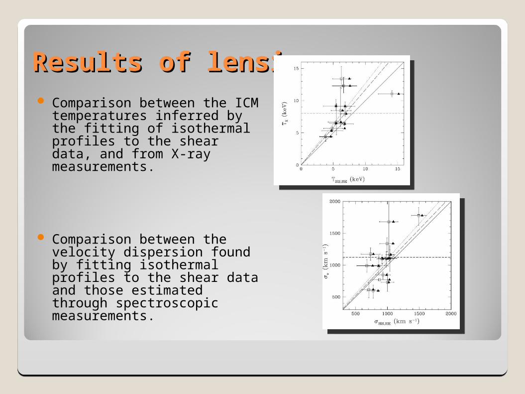
Results of lensing Results of lensing Comparison between the ICM

temperatures inferred by the fitting of isothermal profiles to the shear data, and from X-ray measurements.

Comparison between the velocity dispersion found by fitting isothermal profiles to the shear data and those estimated through spectroscopic measurements.