konza prairie long-term ecological research station tall grass prairie ecosystem
TRANSCRIPT
Konza Prairie Long-Term Ecological Research Station
Tall Grass Prairie Ecosystem
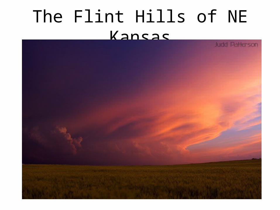
The Flint Hills of NE Kansas
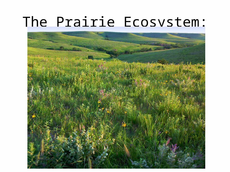
The Prairie Ecosystem:
Long-Term Ecological Research – Konza Prairie
• Konza Prairie Biological Station• Interdisciplinary research program• Est. 1971• 1 of 6 original field stations established to
document temporal & spatial trends across biomes
Konza Prairie Ecosystem
• 3487 hectares (ha) unplowed tallgrass prairie (1 hectare = 2.5 acres)
• Dominated by perennial warm season grasses (as opposed to cool season grasses…)
• Supports diverse community of over 500 other species – herbaceous forbs (=wildflowers), woody shrubs, trees
Konza Prairie Ecosystem
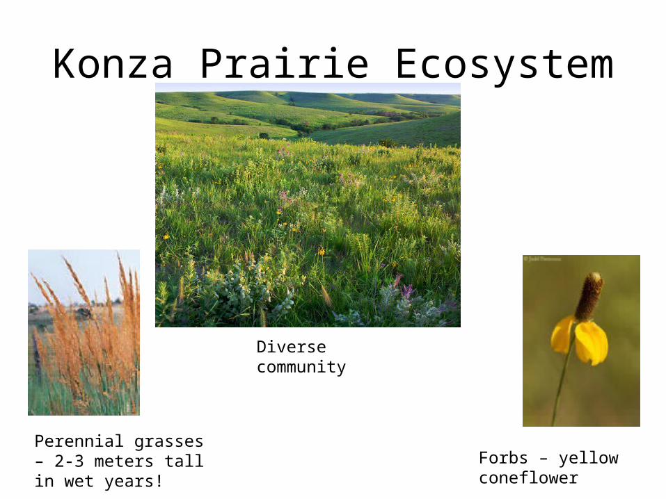
Perennial grasses – 2-3 meters tall in wet years! Forbs – yellow coneflower
Diverse community
Konza Prairie Ecosystem
• Temperate climate, periodic drought, large seasonal & interannual variation in rainfall
• Cold dry winters; warm wet summers• Largest remaining area of unplowed tallgrass
prairie in N. Amer.– Only 5% of area once covered still remains
Konza Prairie Ecosystem
• Experimental design at station:– Divided into 60 watersheds– To study 3 critical factors in maintaining tallgrass
prairie
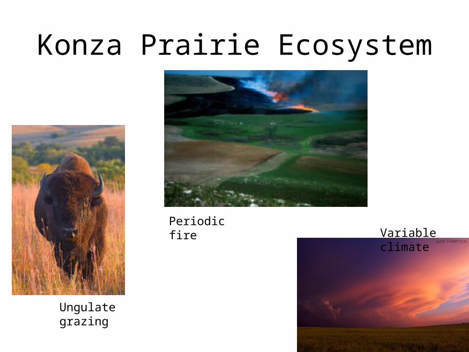
Konza Prairie Ecosystem
Ungulate grazing
Periodic fireVariable climate
Konza Prairie Ecosystem
• Focus of this exercise:• Explore concept of ecological constraints or
limiting factors• What are the main limiting factors on plant
growth in the tallgrass prairie?• Brainstorm…• How do these factors interact?
Konza Prairie Ecosystem
• Compare:• Yearly changes in precipitation• With rate of growth for grasses & forbs• In a 16 year dataset
Konza Prairie Ecosystem
• Biological measurements:– Plant Growth
• How do we measure this?• “Total Primary Productivity”
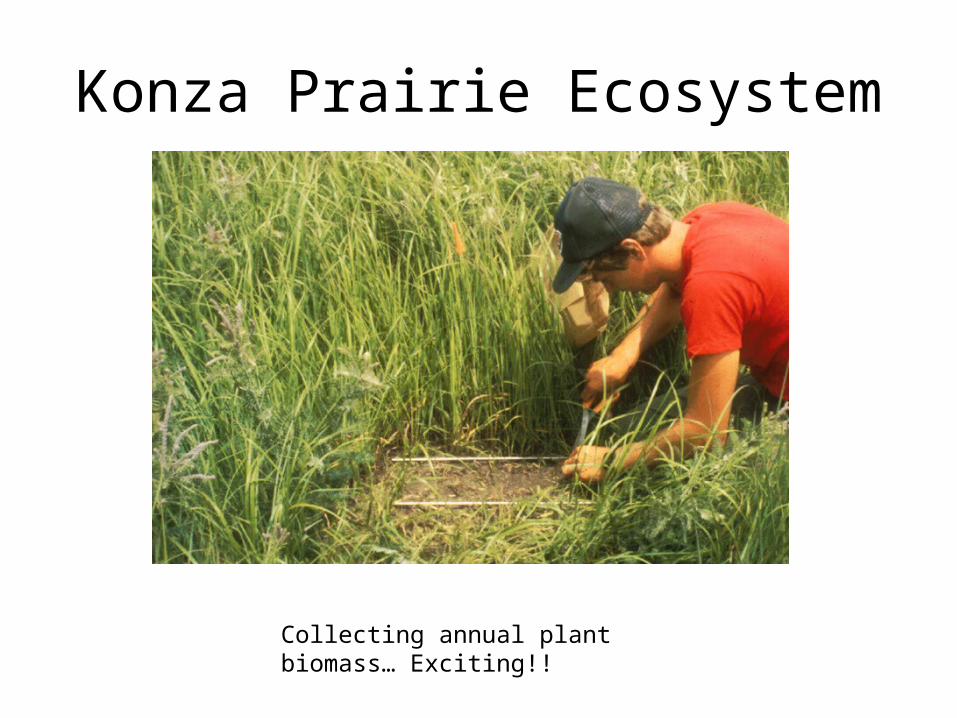
Konza Prairie Ecosystem
Collecting annual plant biomass… Exciting!!
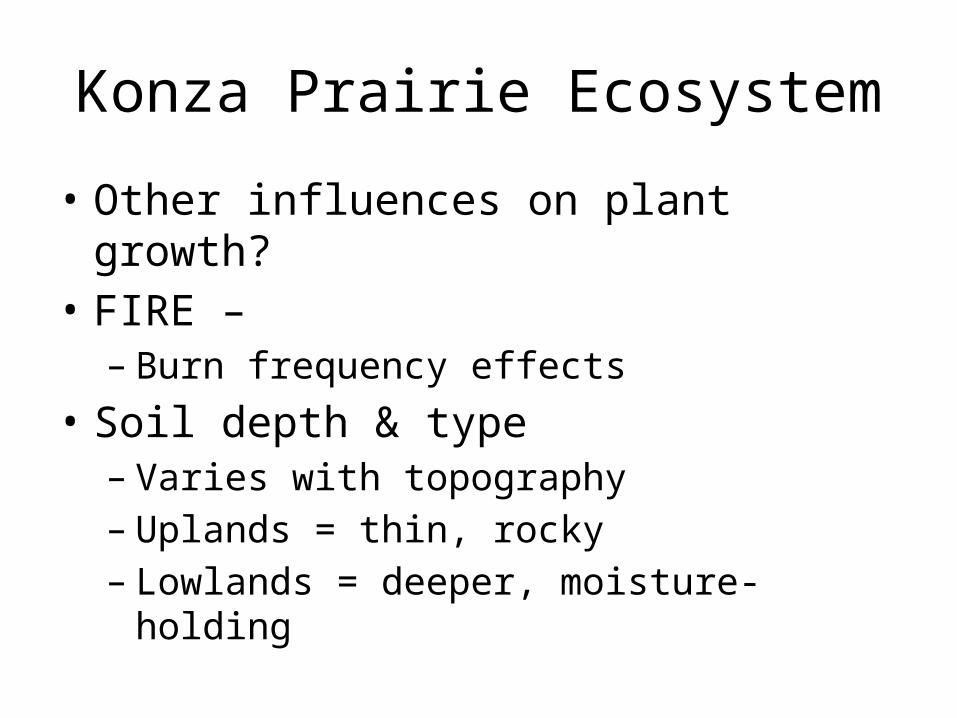
Konza Prairie Ecosystem
• Other influences on plant growth?• FIRE –
– Burn frequency effects• Soil depth & type
– Varies with topography– Uplands = thin, rocky– Lowlands = deeper, moisture-holding
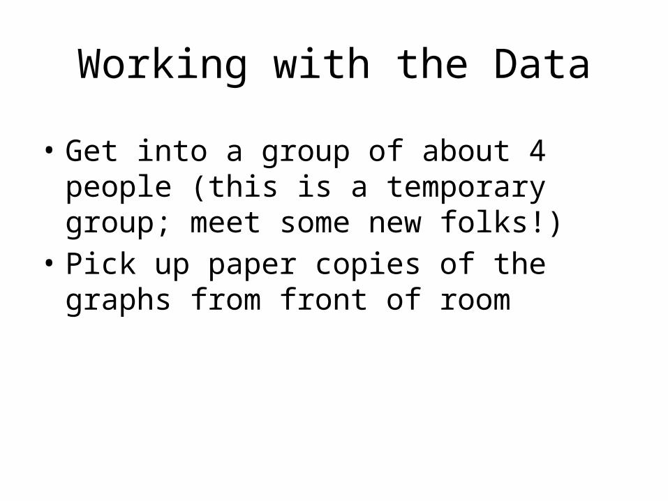
Working with the Data
• Get into a group of about 4 people (this is a temporary group; meet some new folks!)
• Pick up paper copies of the graphs from front of room
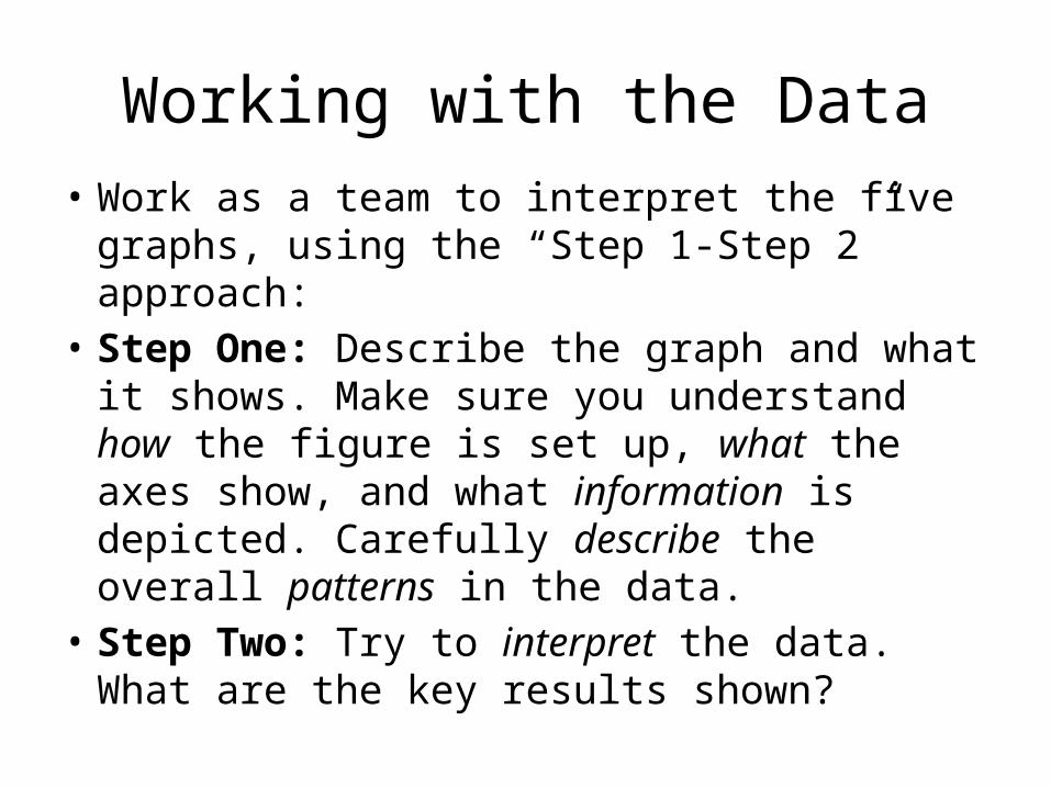
Working with the Data• Work as a team to interpret the five graphs,
using the “Step 1-Step 2” approach:• Step One: Describe the graph and what it
shows. Make sure you understand how the figure is set up, what the axes show, and what information is depicted. Carefully describe the overall patterns in the data.
• Step Two: Try to interpret the data. What are the key results shown?
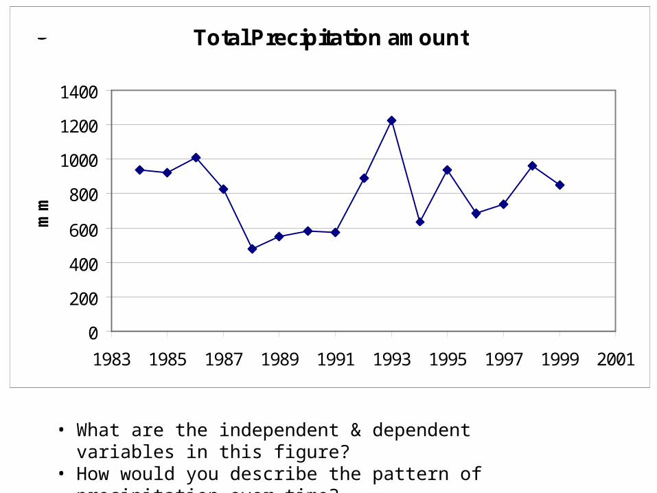
Total Precipitation amount
0
200
400
600
800
1000
1200
1400
1983 1985 1987 1989 1991 1993 1995 1997 1999 2001
mm
Figure 1
• What are the independent & dependent variables in this figure?• How would you describe the pattern of precipitation over time?
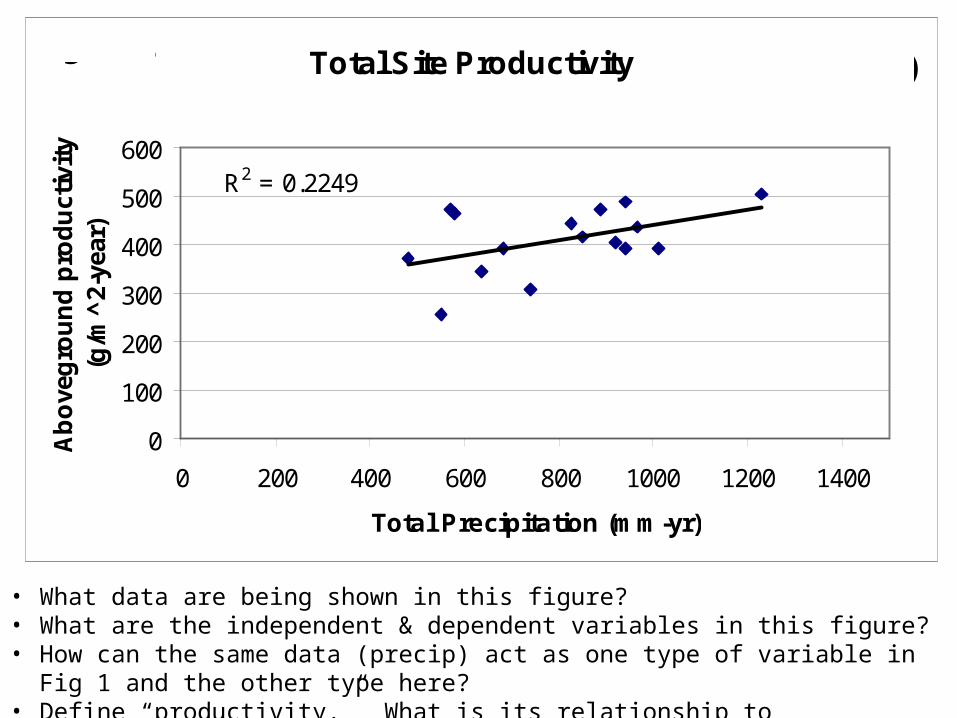
Total Site Productivity
R2 = 0.2249
0
100
200
300
400
500
600
0 200 400 600 800 1000 1200 1400
Total Precipitation (mm-yr)
Ab
ove
gro
un
d p
rod
uct
ivit
y (g
/m^
2-ye
ar)
Figure 2(1984-1999)
• What data are being shown in this figure?• What are the independent & dependent variables in this figure?• How can the same data (precip) act as one type of variable in Fig 1 and the other type here?• Define “productivity.” What is its relationship to precipitation? Does this make sense to you?
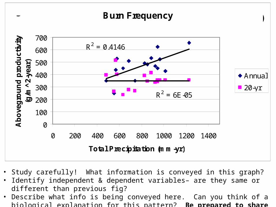
Burn Frequency
R2 = 0.4146
R2 = 6E-05
0
100
200
300
400
500
600
700
0 200 400 600 800 1000 1200 1400
Total Precipitation (mm-yr)
Ab
ove
gro
un
d p
rod
uct
ivit
y (g
/m^
2-ye
ar)
Annual
20-yr
Figure 3(1984-1999)
• Study carefully! What information is conveyed in this graph?• Identify independent & dependent variables– are they same or different than previous fig?• Describe what info is being conveyed here. Can you think of a biological explanation for this
pattern? Be prepared to share with the class!
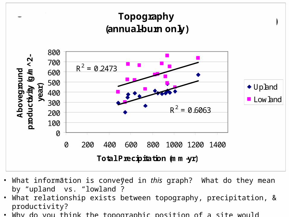
Topography (annual-burn only)
R2 = 0.6063
R2 = 0.2473
0100200300400500600700800
0 200 400 600 800 1000 1200 1400
Total Precipitation (mm-yr)
Ab
ove
gro
un
d
pro
du
ctiv
ity
(g/m
^2-
year
) Upland
Lowland
Figure 4(1984-1999)
• What information is conveyed in this graph? What do they mean by “upland” vs. “lowland”?• What relationship exists between topography, precipitation, & productivity?• Why do you think the topographic position of a site would affect its response to
precipitation?
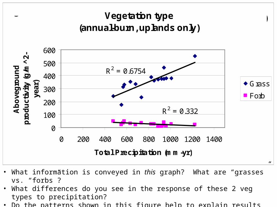
Vegetation type (annual-burn, uplands only)
R2 = 0.6754
R2 = 0.332
0
100
200
300
400
500
600
0 200 400 600 800 1000 1200 1400
Total Precipitation (mm-yr)
Ab
ove
gro
un
d
pro
du
ctiv
ity
(g/m
^2-
year
) Grass
Forb
Figure 5(1984-1999)
• What information is conveyed in this graph? What are “grasses” vs. “forbs”?• What differences do you see in the response of these 2 veg types to precipitation?• Do the patterns shown in this figure help to explain results shown in any of the other graphs?
(hint: look back now at Fig. 3!)
NOW put everything together from the whole data set:
• What biological data are presented?• Which data represent potential constraining
variables?• Can the variables be ranked hierarchically, in terms
of the scale of their influence? Do some variables operate at a larger, regional scale, while some are more local?
• Which vegetation type under what combination of other factors is most strongly influenced by precipitation?
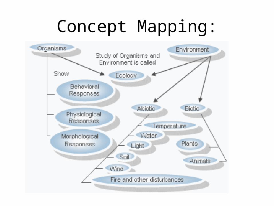
Concept Mapping:
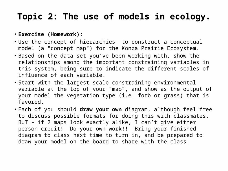
Topic 2: The use of models in ecology.
• Exercise (Homework):• Use the concept of hierarchies to construct a conceptual model (a
"concept map") for the Konza Prairie Ecosystem.• Based on the data set you've been working with, show the relationships
among the important constraining variables in this system, being sure to indicate the different scales of influence of each variable.
• Start with the largest scale constraining environmental variable at the top of your "map", and show as the output of your model the vegetation type (i.e. forb or grass) that is favored.
• Each of you should draw your own diagram, although feel free to discuss possible formats for doing this with classmates. BUT – if 2 maps look exactly alike, I can’t give either person credit! Do your own work!! Bring your finished diagram to class next time to turn in, and be prepared to draw your model on the board to share with the class.