HAL Id: hal-00009125https://hal.archives-ouvertes.fr/hal-00009125

Submitted on 28 Sep 2005

HAL is a multi-disciplinary open accessarchive for the deposit and dissemination of sci-entific research documents, whether they are pub-lished or not. The documents may come fromteaching and research institutions in France orabroad, or from public or private research centers.

L’archive ouverte pluridisciplinaire HAL, estdestinée au dépôt et à la diffusion de documentsscientifiques de niveau recherche, publiés ou non,émanant des établissements d’enseignement et derecherche français ou étrangers, des laboratoirespublics ou privés.

Hardy type inequalitiesJuan Davila, Louis Dupaigne

To cite this version:Juan Davila, Louis Dupaigne. Hardy type inequalities. Journal of the European Mathematical Society,European Mathematical Society, 2004, 6, pp.335–365. �hal-00009125�

J. Eur. Math. Soc. 6, 1–31 c© European Mathematical Society 2004

J. Davila · L. Dupaigne

Hardy-type inequalities

Received March 18, 2003 and in revised form September 15, 2003

1. Introduction

The well-known Hardy–Sobolev inequality states that for any given domain� ⊂ Rn,n ≥ 3 and anyu ∈ C∞

c (�),

K2∫

�

u2

|x|2≤

∫�

|∇u|2, (1)

whereK = (n − 2)/2. Though the constantK2 is optimal, in the sense that

K2= inf

u∈C∞c (�)\{0}

∫�

|∇u|2∫

�u2/|x|2

,

equality in (1) is never achieved (by anyu ∈ H 10 (�)). This fact has led to the improvement

of the inequality in various ways: Brezis and Vazquez [BV] first showed that if� isbounded then for someγ > 0,

γ

(∫�

|u|p

)2/p

+ K2∫

�

u2

|x|2≤

∫�

|∇u|2, (2)

with 1 ≤ p < 2n/(n − 2). Vazquez and Zuazua [VZ] were then able to replace theLp

norm on the left hand side of (2) by aW1,q norm forq < 2. Various improvements (in-volving e.g. weightedLp or W1,p norms) were also obtained and we refer the interestedreader to [Da], [ACR], [FT], [BFT] and the references therein.

One of the consequences of inequality (2) is that the operatorL0 := −1 − µ/|x|2

has a positive first eigenvalue, in the sense that

inf‖u‖

L2(�)=1

∫�

(|∇u|

2− µ

u2

|x|2

)> 0,

wheneverµ ≤ K2.

Research of J. Davila partially supported by Fondecyt 1020815.

J. Davila: Departamento de Ingenieria Matematica, CMM (UMR CNRS), Universidad de Chile,Casilla 170/3 Correo 3, Santiago, Chile; e-mail: jdavila@dim.uchile.cl

L. Dupaigne: Laboratoire Jacques-Louis Lions, Universite Pierre et Marie Curie, Boıte courrier187, 75252 Paris Cedex 05, France; e-mail: dupaigne@ann.jussieu.fr

2 J. Davila, L. Dupaigne

In the first part of this work, given a compact smooth boundaryless manifold6 ⊂ �

of codimensionk 6= 2, we look at operators of the form

L = −1 −µ

d(x)2,

whered(x) = dist(x, 6) andµ ∈ R, and wonder whether an inequality similar to (2)holds.

The first results in this direction are due to Marcus, Mizel and Pinchover [MMP]and Matskewich and Sobolevskii [MSo]. They showed that if� is a convex domain and6 = ∂� then

1

4

∫�

u2

d(x)2≤

∫�

|∇u|2. (3)

The same authors showed that (3) did not hold in a general domain� and providedexamples of smooth domains� such that

infu6≡0

∫�

|∇u|2∫

�u2/d2

<1

4.

Alternatively, Brezis and Marcus showed in [BM] that the following inequality remainstrue on a general (smooth bounded) domain�:

1

4

∫�

u2

d2≤

∫�

|∇u|2+ C

∫�

u2,

whereC is some positive constant.Finally, among many other results, Barbatis, Filippas and Tertikas [BFT, FT] extended

(3) to the case where6 ⊂ � is a smooth compact manifold of codimensionk, satisfyingsome geometric condition: they showed that if1d2−k

≤ 0 inD′(� \ 6) then

γ

(∫�

|u|p

)2/p

+ H 2∫

�

u2

d2≤

∫�

|∇u|2,

whereH = (k − 2)/2 and 1≤ p < 2n/(n − 2).Our goal here is to drop the assumption1d2−k

≤ 0. Our results are summarized inthe following two theorems:

Theorem 1. Let � ⊂ Rn be an open bounded set and6 ⊂ � be a compact smoothmanifold without boundary of codimensionk 6= 2. LetH = (k − 2)/2. Then there existp > 2 andC > 0, γ > 0 independent ofu such that for anyu ∈ C∞

c (� \ 6),

γ

(∫�

|u|p

)2/p

+ H 2∫

�

u2

d2≤

∫�

|∇u|2+ C

∫�

u2, (4)

whered(x) = dist(x, 6), 1 ≤ p < pk andpk is given by

1

pk

=1

2−

2

k(n − k + 2)for k > 2,

1

p1=

1

2−

1

n + 1if k = 1.

Hardy-type inequalities 3

Theorem 2. Under the assumptions of Theorem1, there existβ > 0 and a neighborhood�β := {x ∈ � : d(x, 6) < β} of 6 in � such that for anyu ∈ C∞

c (�β \ 6),

H 2∫

�

u2

d2≤

∫�

|∇u|2. (5)

Remark 1. • If k ≥ 3 it follows by density that (4) and (5) hold for allu ∈ C∞c (�).

• The exponentpk appearing in Theorem 1 is probably not optimal and we expect that(4) holds for all 1≤ p < 2n/(n − 2). In fact Maz’ja [Ma, Corollary 3, Section 2.1.6]proved this result when6 = {x ∈ Rn : x1 = x2 = · · · = xk = 0}.

As a direct consequence of Theorem 1, we see that the first eigenvalue of the operatorL = −1 − µ d−2 is finite, i.e.

λ1 := inf‖u‖

L2(�)=1

∫�

(|∇u|

2− µ

u2

d2

)> −∞,

wheneverµ ≤ H 2. We proved in [DD] that in such circumstances there exists an eigen-functionϕ1 associated toλ1, i.e. a solution (in a sense which we shall make precise soon)of −1ϕ1 −

µ

d2ϕ1 = λ1ϕ1 in �,

ϕ1 = 0 on∂�.

Normalizingϕ1 by ‖ϕ1‖L2(�) = 1 andϕ1 > 0, we then investigate the behavior ofϕ1near6 and show that in a neighborhood of6, there exist constantsC1, C2 > 0 such that

C1d(x)−α(µ)≤ ϕ1 ≤ C2d(x)−α(µ), (6)

whereα(µ) = H −

√H 2 − µ.

This result enables us to treat two model applications. First we consider the quantity

Jλ := infu6≡0

∫�

|∇u|2− λ

∫�

u2∫�

u2/d2

and extend a result of Brezis and Marcus [BM] stating thatJλ is achieved if and only ifJλ < H 2.

Our second application is a nonexistence result for positive solutions of the equation

−1u −µ

d2u = up

+ λ,

completing a study started in [DN]. See Section 4.2 for details.The last purpose of this article is to extend some results in [DD]. This generalization

is necessary to include the case of potentialsa(x) = µ dist(x, 6)−2. More precisely, weshall derive estimates for solutions of the linear equation{

−1u − a(x)u = f in �,

u = 0 on∂�,(7)

4 J. Davila, L. Dupaigne

under the assumptions thata ∈ L1loc(�), a is bounded below, i.e.

ess inf�

a > −∞,

and

γ

(∫�

|u|r

)2/r

+

∫�

a(x)u2≤

∫�

|∇u|2+ M

∫�

u2, (8)

for somer > 2, γ > 0, M > 0.Let us now clarify what we mean by a solution of (7).We first define the Hilbert spaceH as the completion ofC∞

c (�) with respect to thenorm

‖u‖2H = (u|u)H :=

∫�

(|∇u|2− a(x)u2

+ Mu2),

whereM is the same constant that appears in (8). Observe that the definition ofH doesnot change if we replaceM by any larger constant.

Givenf ∈ H∗, we then say thatu ∈ H is a solution of (7) if

(u|v)H = 〈f, v〉H∗,H + M(u|v)L2(�) ∀v ∈ H.

It is convenient at this point to recall some facts that were proved in [DD]. We startby mentioning thatH embeds compactly inL2(�). In particular

L = −1 − a(x)

has a first eigenvalueλ1, which is simple.λ1 is not necessarily positive (Theorem 1 pro-vides examples of potentialsa(x) = H 2/d(x)2 for which in generalλ1 can be nonposi-tive), but when it is, then forf ∈ H∗ problem (7) has a unique solutionu ∈ H.

We note here that uniqueness fails if one considers other classes of solutions (see anexample in [DD]).

The first eigenvalueλ1 has an associated positive eigenfunctionϕ1 (it is not onlypositive a.e. but it also satisfiesϕ1 ≥ c dist(x, ∂�) for somec > 0).

Solutions inH of an equation like (7) are typically unbounded (see examples in [D,DD, DN]). In [DD] we showed that ifλ1 > 0 andf ≥ 0, f 6≡ 0 then the solutionu ∈ Hof (7) is bounded below by a positive constant timesϕ1. We also proved that ifλ1 > 0andf = 1, then the solutionu of (7) satisfiesu ≤ Cϕ1 for someC > 0.

Our main result is the following:

Theorem 3. Let0 < m < r and suppose that

p >2r

m(r − 2)and p ≥

r

r − m.

Assume thatf ∈ H∗ satisfies‖ϕ1−m1 f ‖Lp(�) < ∞ and thatu ∈ H is a solution of(7).

Then|u(x)| ≤ C(‖ϕ1−m

1 f ‖Lp(�) + ‖u‖L2(�))ϕ1(x), a.e.x ∈ �.

Hardy-type inequalities 5

A simple corollary of this result, obtained by choosingm = 2, is the following:

Corollary 1. Assumef ∈ H∗ satisfiesf/ϕ1 ∈ Lp(�) for somep > r/(r − 2) and thatu ∈ H is a solution of(7). Then

|u(x)| ≤ C(‖f/ϕ1‖Lp(�) + ‖u‖L2(�))ϕ1(x), a.e.x ∈ �.

The paper is organized as follows: Section 2 is devoted to the proof of Theorems 1 and 2.In Section 3 we derive (6) whereas Section 4 is dedicated to the aforementioned applica-tions. Finally, we prove Theorem 3 in Section 5.

2. Hardy inequalities

2.1. Proof of Theorem 1

The object of this subsection is to prove Theorem 1. Our arguments are based on improve-ments of the one-dimensional Hardy inequality inspired by [BM] and a decomposition ofL2 functions in spherical harmonics taken from [VZ].

We start with a series of three lemmas, which yield a refined version of the classicalHardy inequality inRk (see (3)). The first lemma deals with radial functions:

Lemma 1. Letk 6= 2 andH = (k − 2)/2. There exists a constantC > 0 depending onlyonk such that∫ 1/2

0

[(du

dr

)2

− H 2u2

r2

]rk−1 dr + C

∫ 1/2

0u2rk−1 dr

≥

∫ 1/2

0

[(du

dr

)2

+ H 2u2

r2

]rk dr +

1

4

∫ 1/2

0r

(d

dr(rH u(r))

)2

dr (9)

for all u ∈ C∞c (0, 1/2).

Proof. Let u ∈ C∞c (0, 1/2) andv(r) = rH u(r). A standard computation yields[(

du

dr

)2

− H 2u2

r2

]rk−1

= r

(dv

dr

)2

− Hd(v2)

dr. (10)

Integrating, it follows that

A :=∫ 1/2

0

[(du

dr

)2

− H 2u2

r2

]rk−1 dr =

∫ 1/2

0r

(dv

dr

)2

dr. (11)

Similarly, by (10) and an integration by parts,

B :=∫ 1/2

0

[(du

dr

)2

+ H 2u2

r2

]rk dr

=

∫ 1/2

0r2

(dv

dr

)2

dr + 2H 2∫ 1/2

0

u2

r2rk dr − H

∫ 1/2

0r

[d(v2)

dr

]dr

=

∫ 1/2

0r2

(dv

dr

)2

dr + (2H 2+ H)

∫ 1/2

0v2 dr. (12)

6 J. Davila, L. Dupaigne

Using integration by parts again, it follows that for givenε > 0, there existsC > 0 suchthat∫ 1/2

0v2 dr = −2

∫ 1/2

0rv

dv

drdr ≤ C

∫ 1/2

0v2r dr + ε

∫ 1/2

0

(dv

dr

)2

r dr

= C

∫ 1/2

0u2rk−1 dr + ε

∫ 1/2

0

(dv

dr

)2

r dr. (13)

Collecting (11), (12) and (13), we obtain forε small enough

A − B ≥

∫ 1/2

0r(1 − r − Cε)

(dv

dr

)2

dr − C

∫ 1/2

0u2rk−1 dr

≥1

4

∫ 1/2

0r

(dv

dr

)2

dr − C

∫ 1/2

0u2rk−1 dr. �

The next lemma will help us deal with the nonradial part of a given functionu : Rk→ R.

Lemma 2. Let k 6= 2, H = (k − 2)/2 andc > c > 0. There exist constantsC, τ > 0depending only onk and c such that∫ 1/2

0

[(du

dr

)2

− (H 2− c)

u2

r2

]rk−1 dr + C

∫ 1/2

0u2rk−1 dr

≥

∫ 1/2

0

[(du

dr

)2

+ (H 2+ c)

u2

r2

]rk dr + τ

∫ 1/2

0

[(du

dr

)2

+ cu2

r2

]rk−1 dr (14)

for all u ∈ C∞c (0, 1/2).

Proof. It follows from (9) that if

D :=∫ 1/2

0

[(du

dr

)2

− (H 2− c)

u2

r2

]rk−1 dr + C

∫ 1/2

0u2rk−1 dr (15)

and

E :=∫ 1/2

0

[(du

dr

)2

+ (H 2+ c)

u2

r2

]rk dr (16)

then

D − E ≥ c

∫ 1/2

0

u2

r2(1 − r)rk−1 dr +

1

4

∫ 1/2

0r

(dv

dr

)2

dr

≥c

2

∫ 1/2

0

u2

r2rk−1 dr +

1

4

∫ 1/2

0r

(dv

dr

)2

dr. (17)

Hardy-type inequalities 7

We can also rewrite (10) as

rk−1(

du

dr

)2

= H 2u2

r2rk−1

+ r

(dv

dr

)2

− Hd(v2)

dr

so that ifτ = min(

c

4H2 , 14

), then

τ

∫ 1/2

0rk−1

(du

dr

)2

dr ≤c

4

∫ 1/2

0

u2

r2rk−1 dr +

1

4

∫ 1/2

0r

(dv

dr

)2

dr. (18)

It then follows from (17) and (18) that

D − E ≥ τ

∫ 1/2

0rk−1

(du

dr

)2

dr +c

4

∫ 1/2

0

u2

r2rk−1 dr. (19)

Hence (2) holds. �

Finally, the following lemma yields the improved Hardy inequality (inRk) that wewill be using in what follows.

Lemma 3. Letk 6= 2, H = (k − 2)/2 andβ > 0. LetBkβ denote the ball ofRk centered

at the origin and of radiusβ. There exist positive constantsC = C(β, k), τ = τ(k) andα = α(β, k) such that∫

Bkβ

(|∇u|

2− H 2 u2

|y|2

)dy + C

∫Bk

β

u2 dy

≥1

2β

∫Bk

β

|y|

(|∇u|

2+H 2 u2

|y|2

)dy+τ

∫Bk

β

|∇(u − u0)|2 dy+α

∫ β

0r

(dv0

dr

)2

dr (20)

for all u ∈ C∞c (Bk

β \ {0}), whereu0(r) = u0(|y|) = −

∫∂Bk

ru dσ andv0(r) = rH u0(r).

Proof. Let {fi}∞

i=0 be an orthonormal basis ofL2(Sk−1), composed of eigenvectors ofthe Laplace–Beltrami operator1|Sk−1. The corresponding eigenvalues are given byci =

i(k + i − 2), i = 0, 1, 2, . . . (see e.g. [St]). Anyu ∈ C∞c (Bk

1/2 \ {0}) can then be writtenas

u(x) =

∞∑i=0

ui(r)fi(θ)

where 1/2 > r > 0, θ ∈ Sk−1 andx = rθ .Furthermore, forg ∈ C(R+, R),∫

Bk1/2

|∇u|2 g(|y|) dy =

∫ 1/2

0rk−1g(r) dr

∫Sk−1

[(∂u

∂r

)2

+1

r2|∇θu|

2]dθ

=

∞∑i=0

∫ 1/2

0rk−1g(r)

[(dui

dr

)2

+ci

r2u2

i

]dr. (21)

8 J. Davila, L. Dupaigne

For i = 0, it follows from (9) that ifv0(r) = rH u0(r), then∫ 1/2

0

[(du0

dr

)2

− H 2u20

r2

]rk−1 dr + C

∫ 1/2

0u2

0rk−1 dr

≥

∫ 1/2

0

[(du0

dr

)2

+ H 2u20

r2

]rk dr +

1

4

∫ 1/2

0r

(dv0

dr

)2

dr, (22)

while (2) implies that fori ≥ 1,∫ 1/2

0

[(dui

dr

)2

− (H 2− ci)

u2i

r2

]rk−1 dr + C

∫ 1/2

0u2

i rk−1 dr

≥

∫ 1/2

0

[(dui

dr

)2

+ (H 2+ ci)

u2i

r2

]rk dr + τ

∫ 1/2

0

[(dui

dr

)2

+ cu2

i

r2

]rk−1 dr. (23)

Using (22), (23) and (21) withg(r) ≡ 1 for terms involvingrk−1 andg(r) = r for termswith rk, we deduce (3) forβ = 1/2. The general case is obtained by scaling. �

Next, we introduce some geometric notation that will be needed in the proof of Theo-rem 1. Define

�β = { x ∈ � | dist(x, 6) < β }.

We will work only with β small enough so that the projectionπ : �β → 6 given by|π(x) − x| = dist(x, 6) is well defined and smooth.

Let {Vi}i=1,...,m be a family of open disjoint subsets of6 such that

6 =

m⋃i=1

V i, |V i ∩ Vj | = 0 ∀i 6= j.

We can also assume that:

(a) ∀i = 1, . . . , m there exists a smooth diffeomorphism

pi : Bn−k1 → Ui,

whereUi ⊂ 6 is open andV i ⊂ Ui ;(b) p−1

i (Vi), which is an open set inRn−k, has a Lipschitz boundary; and(c) there is a smooth choice of unit vectorsN i

1(σ ), . . . , N ik(σ ) for σ ∈ Ui which form

an orthonormal frame for6 onUi ⊂ Rn , i.e. for allσ ∈ Ui ,

N ij (σ ) ∈ Rn, N i

j (σ ) · N ik(σ ) = δjk, N i

j (σ ) · v = 0 ∀v ∈ Tσ 6.

Let Wi = p−1i (Vi). For z ∈ Wi we will also write (abusing the notation)N i

j (z) =

N ij (pi(z)). Let

Fi(y, z) = pi(z) +

k∑j=1

yjNij (z),

wherey = (y1, . . . , yk) ∈ Bkβ andz ∈ Wi , so thatFi is a smooth diffeomorphism between

Bkβ × Wi andT i

β , where

T iβ = π−1(Vi) ∩ �β . (24)

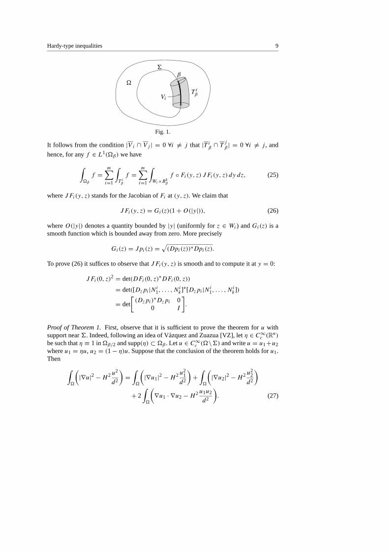
Hardy-type inequalities 9

�

6

Vi

T iβ

β

Fig. 1.

It follows from the condition|V i ∩ Vj | = 0 ∀i 6= j that |T iβ ∩ T

jβ | = 0 ∀i 6= j , and

hence, for anyf ∈ L1(�β) we have∫�β

f =

m∑i=1

∫T i

β

f =

m∑i=1

∫Wi×Bk

β

f ◦ Fi(y, z) JFi(y, z) dy dz, (25)

whereJFi(y, z) stands for the Jacobian ofFi at (y, z). We claim that

JFi(y, z) = Gi(z)(1 + O(|y|)), (26)

whereO(|y|) denotes a quantity bounded by|y| (uniformly for z ∈ Wi) andGi(z) is asmooth function which is bounded away from zero. More precisely

Gi(z) = Jpi(z) =√

(Dpi(z))∗Dpi(z).

To prove (26) it suffices to observe thatJFi(y, z) is smooth and to compute it aty = 0:

JFi(0, z)2= det(DFi(0, z)∗DFi(0, z))

= det([Dzpi |Ni1, . . . , N

ik]∗[Dzpi |N

i1, . . . , N

ik])

= det

[(Dzpi)

∗Dzpi 00 I

].

Proof of Theorem 1.First, observe that it is sufficient to prove the theorem foru withsupport near6. Indeed, following an idea of Vazquez and Zuazua [VZ], letη ∈ C∞

c (Rn)

be such thatη ≡ 1 in �β/2 and supp(η) ⊂ �β . Letu ∈ C∞c (�\6) and writeu = u1+u2

whereu1 = ηu, u2 = (1− η)u. Suppose that the conclusion of the theorem holds foru1.Then ∫

�

(|∇u|

2− H 2 u2

d2

)=

∫�

(|∇u1|

2− H 2 u2

1

d2

)+

∫�

(|∇u2|

2− H 2 u2

2

d2

)+ 2

∫�

(∇u1 · ∇u2 − H 2u1u2

d2

). (27)

10 J. Davila, L. Dupaigne

Since 1/d is bounded away from6 we have∫�

(u2

2

d2+

u1u2

d2

)≤ C

∫�

u2.

Also note that∫�

∇u1 · ∇u2 =

∫�

[η(1 − η)|∇u|2− |∇η|

2u2+ u∇u · ∇η(1 − 2η)]

=

∫�

[η(1 − η)|∇u|2− |∇η|

2u2] −1

2

∫�β\�β/2

u2∇ · (∇η(1 − 2η))

≥ −C

∫�

u2. (28)

It follows from (27), (28) that∫�

[|∇u|

2− H 2 u2

d2

]≥

∫�

[|∇u1|

2− H 2 u2

1

d2

]+

∫�

|∇u2|2− C

∫�

u2.

Using (4) withu1 we conclude that∫�

[|∇u|

2− H 2 u2

d2

]+ C

∫�

u2≥ γ

( ∫�

|u1|p

)2/p

+

∫�

|∇u2|2,

for someγ > 0 independent ofu. Hence the conclusion of the theorem foru followseasily.

Let

Ii =

∫T i

β

[|∇u|

2− H 2 u2

d2+ u2

], (29)

whereT iβ was defined in (24). In what follows we will fixi and show that there arep > 2

andC > 0 independent ofu such that(∫T i

β

|u|p

)2/p

≤ CIi .

For simplicity, and sincei is fixed, we will drop the indexi from all the notation thatfollows.

Let us introduce some additional notation:

u(y, z) = u(F (y, z)), (30)

u0(r, z) = −

∫∂Br

u(y, z) ds(y), (31)

v0(r, z) = rH u0(r, z). (32)

Let us write∇u = ∇N u + ∇T u

Hardy-type inequalities 11

where∇N u is the gradient ofu in the normal direction and∇T u is orthogonal to∇N u.More precisely, for a pointx = F(y, z),

∇N u(x) =

k∑j=1

∇u(x) · Nj (z) Nj (z).

Step 1.There existsC > 0 independent ofu such that

CI ≥

∫W×Bk

β

|∇y u|2|y| dy dz +

∫W×Bk

β

|∇y(u(y, z) − u0(y, z))|2 dy dz

+

∫W

∫ β

0

(∂v0

∂r

)2

r dr dz +

∫W×Bk

β

|(∇T u) ◦ F |2 dy dz. (33)

First note that by (25), there is a constantC > 0 such that

I ≥

∫W×Bk

β

(|∇N u(F (y, z))|2 − H 2 u2

|y|2

)G(z) dy dz

− C

∫W×Bk

β

(|∇N u(F (y, z))|2 + H 2 u2

|y|2

)G(z)|y| dy dz

+

∫W×Bk

β

(|∇T u(F (y, z))|2 + u2)(1 − C|y|)G(z) dy dz. (34)

For fixedz we can apply Lemma 3 to the functionu(·, z). Observe that

∂u(y, z)

∂yj

= ∇u(F (y, z)) · Nj (z)

and thus|∇y u(y, z)|2 = |∇N u(F (y, z))|2.

Lemma 3 then yields∫Bk

β

(|∇N u(F (y, z))|2 − H 2 u2

|y|2

)dy + C

∫Bk

β

u2 dy

≥1

2β

∫Bk

β

|y|

(|∇N u(F (y, z))|2 + H 2 u2

|y|2

)dy

+ τ

∫Bk

β

∣∣∇y(u − u0)∣∣2 dy + α

∫ β

0r

(dv0

dr

)2

dr. (35)

We choose (and fix once for all)β > 0 small enough so that 1/(2β) ≥ C + 1. Thenmultiplying (35) by G(z), integrating overW and combining the result with (34) weconclude that (33) holds.

12 J. Davila, L. Dupaigne

Step 2.‖∇v0‖

2L2(W×B2

β )≤ CI. (36)

By (33) the partial derivative∂v0/∂r is bounded inL2(W × B2β) by CI . We just have to

control the derivatives∂v0/∂zi , i = 1, . . . , n − k. But

∂v0

∂zi

(r, z) = rH−

∫∂Br

∂u

∂zi

(y, z) ds(y)

and∂u

∂zi

(y, z) = ∇u(F (y, z)) ·

[∂p

∂zi

+

k∑j=1

yj

∂Nj

∂zi

].

But note that∂p/∂zi is a tangent vector, hence

|∇zu(y, z)| ≤ C|∇T u(F (y, z))| + C|y| |∇N u(F (y, z))|.

Integrating overW × Bkβ we have∫

W×Bkβ

|∇zu(y, z)|2 dy dz ≤ CI, (37)

for someC independent ofu by (33). It follows that∫W×B2

β

|∇zv0|2 dy dz =

∫W

∫ β

0r2H+1

∣∣∣∣−∫∂Br

∇zu(y, z) ds(y)

∣∣∣∣2 dr dz

≤

∫W

∫ β

0rk−1

−

∫∂Br

|∇zu(y, z)|2 ds(y) dr dz

≤ C

∫W×Bk

β

|∇zu(y, z)|2 dy dz ≤ CI (38)

by (37).

Step 3.There isp > 2 such that

‖u0‖2Lp(W×Bk

β )≤ CI. (39)

More precisely, fork ≥ 3 one can take any 2< p < pk wherepk is given by

1

pk

=1

2−

2

k(n − k + 2),

and fork = 1 one can take 2< p ≤ p1 wherep1 is given by

1

p1=

1

2−

1

n + 1.

Hardy-type inequalities 13

Using Sobolev’s inequality (onW × B2β ) combined with (36) we obtain

∫W

∫ β

0|v0|

qr dr dz ≤ CI q/2,

with q given by 1/q = 1/2 − 1/(n − k + 2). That is, in terms ofu0 we have∫W

∫ β

0|u0|

qrqH+1 dr dz ≤ CI q/2. (40)

We want an estimate for∫

|u0|prk−1 dr dz for some suitable 2< p < q and for this we

use Holder’s inequality, distinguishing two cases:

Casek ≥ 3. We have

∫W

∫ β

0|u0|

prk−1 dr dz =

∫W

∫ β

0|u0|

prαrk−2−αr dr dz

≤ C

(∫W

∫ β

0|u0|

q rαq/p+1 dr, dz

)p/q(∫ β

0r

k−2−α1−p/q

+1dr

)1−p/q

. (41)

We then chooseα so thatα

p= H =

k − 2

2.

In order to have the second factor on the right hand side of (41) finite we need to impose

k − 2 − α

1 − p/q> −2,

which is equivalent to the condition

α <k

1 +4

q(k−2)

.

Thus we needp = α/H < pk, wherepk is given by

pk =2k

(k − 2)(1 +

4q(k−2)

) ,

i.e.1

pk

=1

2−

2

k(n − k + 2).

Observe thatpk > 2. Combining then (40) and (41) finishes this case.

14 J. Davila, L. Dupaigne

Casek = 1. In this caseq is given by 1/q = 1/2 − 1/n + 1, and we can choosep = q:∫W

∫ β

0|u0|

qrk−1 dr dz =

∫W

∫ β

0|u0|

q dr dz

≤

∫W

∫ β

0|u0|

qr−q/2+1 dr dz

=

∫W

∫ β

0|u0|

qrHq+1 dr dz

because−q/2 + 1 < 0.

Step 4.‖u − u0‖

2L2∗

(W×Bkβ )

≤ CI. (42)

This is a consequence of Sobolev’s inequality applied to the functionu−u0 on the domainW × Bk

β . (33) already provides a bound inL2(W × Bkβ) for ∇y(u − u0). Hence we only

need to obtain a bound for the derivative ofu − u0 with respect toz. In the case of thefunction u we have it already in (37). Foru0 it is derived by a computation very similarto that at the end of Step 2. Indeed,∫

W×Bkβ

|∇zu0|2 dy dz =

∫W

∫ β

0rk−1

∣∣∣∣−∫∂Br

∇zu(y, z) ds(y)

∣∣∣∣2 dr dz ≤ CI,

which we obtain as in (38).

Conclusion.By (39) and (42) we see that

‖u‖2Lp(W×Bk

β )≤ CI

for someC independent ofu. Changing variables and reintroducing the indexi we have

‖u‖2Lp(T i

β )≤ C

∫T i

β

(|∇u|

2− H 2 u2

d2+ u2

).

Adding these inequalities overi proves the statement of the theorem. �

2.2. A local version of the Hardy inequality

In this section, we show how to adapt the proof of Theorem 1 to obtain Theorem 2. Wefirst derive variants of Lemmas 1, 2, 3.

Lemma 4. Let k 6= 2 andH = (k − 2)/2. There exist constantsC, β0 > 0 such that for0 < β ≤ β0,∫ β

0

[(du

dr

)2

− H 2u2

r2

]rk−1 dr ≥

∫ β

0

[(du

dr

)2

+ H 2u2

r2

]rk dr (43)

for all u ∈ C∞c (0, β).

Hardy-type inequalities 15

Proof. Givenv ∈ C∞c (0, 1/2), we have∫ 1/2

0v2 dr = −2

∫ 1/2

0rv

dv

drdr ≤ C

∫ 1/2

0r2

(dv

dr

)2

dr +1

2

∫ 1/2

0v2 dr.

Using this and (12) we obtain∫ 1/2

0

[(du

dr

)2

+ H 2u2

r2

]rk dr ≤ C

∫ 1/2

0r2

(dv

dr

)2

dr.

Changing variables, it then follows that foru ∈ C∞c (0, β),∫ β

0

[(du

dr

)2

+ H 2u2

r2

]rk dr ≤ Cβk−2

∫ β

0r2

(dv

dr

)2

dr, (44)

while (11) becomes∫ β

0

[(du

dr

)2

− H 2u2

r2

]rk−1 dr = βk−2

∫ β

0r

(dv

dr

)2

dr. (45)

If we pick β small, (43) follows from (44) and (45). �

A straightforward corollary of the above lemma is:

Lemma 5. Let k 6= 2, H = (k − 2)/2 andc > 0. There exist constantsC, β0 > 0 suchthat for0 < β ≤ β0,∫ β

0

[(du

dr

)2

− (H 2− c)

u2

r2

]rk−1 dr ≥

∫ β

0

[(du

dr

)2

+ (H 2+ c)

u2

r2

]rk dr (46)

for all u ∈ C∞c (0, β).

Combining these two lemmas, we then obtain:

Lemma 6. Let k 6= 2, H = (k − 2)/2 andβ > 0. LetBkβ denote the ball ofRk centered

at the origin and of radiusβ. There exist positive constantsC, β0 such that forβ ≤ β0,∫Bk

β

(|∇u|

2− H 2 u2

|y|2

)dy ≥

C

β

∫Bk

β

|y|

(|∇u|

2+ H 2 u2

|y|2

)dy (47)

for all u ∈ C∞c (Bk

β \ {0}), whereu0(r) = u0(|y|) = −

∫∂Bk

ru dσ andv0(r) = rH u0(r).

As in Lemma 3, for a fixed valueβ = β0 > 0 the proof is an application of the decompo-sition of a function in spherical harmonics. A simple scaling then yields theβ-dependenceof the constant appearing in (47).

Proof of Theorem 2.Instead of (29), we now consider

Ji :=∫

T iβ

[|∇u|

2− H 2 u2

d2

]. (48)

16 J. Davila, L. Dupaigne

Using the notation of (30) we then have, by (25) and (26),

Ji ≥

∫W×Bk

β

(|∇N u(Fi(y, z))|2 − H 2 u2

|y|2

)G(z) dy dz

− C

∫W×Bk

β

|y|

(|∇N u(Fi(y, z))|2 + H 2 u2

|y|2

)G(z) dy dz ≥ 0,

where we used Lemma 6 withβ > 0 small in the last inequality. Adding the aboveestimates overi yields the desired result. �

3. Remarks on the potentiala(x) = µ dist(x, 6)−2

For 0< µ ≤ H 2 we consider the potential

a(x) = µ/d(x)2

and letL denote the operator

Lu = −1u − a(x)u.

Note thata(x) andL depend onµ but we will omit this dependence from the notation.Recall that we defined the Hilbert spaceH as the completion ofC∞

c (�) with respectto the norm

‖u‖2H =

∫�

(|∇u|2− a(x)u2

+ Mu2). (49)

If µ < H 2 then by Theorem 1,H coincides withH 10 (�).

The main concern in this section is to obtain a precise description of the behavior near6 of the first eigenfunctionϕ1 of the operatorL. Indeed, we shall prove:

Lemma 7. There are positive constantsC1, C2 such that

C1d(x)−α(µ)≤ ϕ1(x) ≤ C2d(x)−α(µ) (50)

for x in a neighborhood of6, whereα(µ) is given by

α(µ) = H −

√H 2 − µ. (51)

Note that whenµ = H 2 we have−α(µ) = 1 − k/2. Thusϕ1 6∈ H 10 (�) in this case.

Before proving the above lemma it will be necessary to show that ifµ = H 2 thend1−k/2

(appropriately modified so that it is zero on∂�) belongs toH. We prove this and a littlemore next.

Lemma 8. Letµ = H 2 and define

vs(x) = η(x)d(x)1−k/2(− logd(x))−s,

whereη ∈ C∞c (�) is a cut-off function such thatη ≡ 1 in a neighborhood of6 and

η(x) = 0 for d(x) ≥ dist(6, ∂�)/2. Thenvs ∈ H if and only ifs > −1/2.

Hardy-type inequalities 17

Remark 2. This lemma was stated in [VZ] in the case where6 is a point.

Proof. Let us recall and also introduce some notation:

�r = {x ∈ RN| d(x) < r}, 6r = ∂�r = { x ∈ RN

| d(x) = r }.

By the Pappus theorems, the(N − 1)-dimensional area of6r is given by

|6r |n−1 = ωk−1rk−1

|6|n−k,

whereωk−1 is the area of the unit sphere inRk and | · |j denotes thej -dimensionalLebesgue measure.

First we prove thatvs ∈ H for s > −1/2. For this purpose it is enough to exhibit asequencefε ∈ H such that‖fε‖H ≤ C with C independent ofε and such thatfε → vs

a.e. asε → 0; we take

fε = ηd1−k/2+ε(− logd)−s, ε > 0.

Clearlyfε ∈ H 10 (�) ⊂ H,

∫�

f 2ε ≤ C andfε is smooth away from6. Thus to estimate

‖fi‖H it is sufficient to verify that for a fixedR > 0 small∫�R

|∇fε|2− a(x)f 2

ε ≤ C (52)

with C independent ofε.Near6, η ≡ 1 and

|∇fε|2

= d−k+2ε((1 − k/2 + ε)2(− logd)−2s

+ s(2 − k + 2ε)(− logd)−2s−1+ s2(− logd)−2s−2).

so that

1

ωk−1|6|n−k

∫�R

|∇fε|2

= (1 − k/2 + ε)2∫ R

0r2ε−1(− logr)−2s dr

+ s(2 − k + 2ε)

∫ R

0r2ε−1(− logr)−2s−1 dr

+ s2∫ R

0r2ε−1(− logr)−2s−2 dr.

Note that the last integral on the right hand side above is bounded independently ofε fors > −1/2, that is, ∫ R

0r2ε−1(− logr)−2s−2 dr = O(1).

18 J. Davila, L. Dupaigne

Therefore

1

ωk−1|6|n−k

∫�R

(|∇fε|

2− H 2f 2

ε

d2

)= ε(2 − k + ε)

∫ R

0r2ε−1(− logr)−2s dr

+ s(2 − k + 2ε)

∫ R

0r2ε−1(− logr)−2s−1 dr + O(1). (53)

Integrating by parts gives∫ R

0r2ε−1(− logr)−2s dr =

1

2εR2ε(− logR)−2s

−s

ε

∫ R

0r2ε−1(− logr)−2s−1 dr

and substituting in (53) yields

1

ωk−1|6|n−k

∫�R

(|∇fε|

2− H 2f 2

ε

d2

)=

2 − k + ε

2R2ε(− logR)−2s

+ εs

∫ R

0r2ε−1(− logr)−2s−1 dr + O(1)

= εs

∫ R

0r2ε−1(− logr)−2s−1 dr + O(1). (54)

Integrating by parts again shows that

∫ R

0r2ε−1(− logr)−2s−1 dr

=1

2εR2ε(− logR)−2s−1

−2s + 1

2ε

∫ R

0r2ε−1(− logr)−2s−2 dr = O

(1

ε

).

After substitution in (54) we finally obtain the estimate (52). Hencevs ∈ H for s > −1/2.Our argument to show thatvs 6∈ H for s ≤ −1/2 relies on the intuitive idea that∫

(−1v − a(x)v + Mv)v = ‖v‖2H. To exploit this idea, let us first compute1vs near6,

whereη ≡ 1. Write

y(t) = t1−k/2(− log t)−s .

Then near6, since|∇d|2

= 1,

1vs = y′′(d) + y′(d)1d.

We recall here the fact (see [DN]) that

1d =k − 1

d+ g,

Hardy-type inequalities 19

whereg ∈ L∞. Hence,

1vs = − H 2d−k/2−1(− logd)−s+ s(s + 1)d−k/2−1(− logd)−s−2

+ (1 − k/2)gd−k/2(− logd)−s+ sgd−k/2(− logd)−s−1

so that

1vs + H 2 vs

d2= s(s + 1)d−k/2−1(− logd)−s−2

+ (1 − k/2)gd−k/2(− logd)−s+ sgd−k/2(− logd)−s−1. (55)

Observe that1vs, vs/d2

∈ L1(�) and that equation (55) holds in the sense of distribu-tions. Since we also have∇vs ∈ L1(�), it follows that for anyϕ ∈ C∞

c (�),

(vs |ϕ)H =

∫�

(−1vs − H 2 v2

s

d2

)ϕ + M

∫�

vsϕ

−

∫�R

(s(s + 1)d−k/2−1(− logd)−s−2

+ (1 − k/2)gd−k/2(− logd)−s+ sgd−k/2(− logd)−s−1)ϕ

+

∫�\�R

(−1vs − H 2 vs

d2

)ϕ + M

∫�

vsϕ. (56)

By density (56) also holds ifϕ is Lipschitz andϕ = 0 on∂�.Let us consider first the cases 6= −1, so thats(s+1) 6= 0, and suppose thats < −1/2

andvs ∈ H. Then there existvn ∈ C∞c (�) such thatvn → vs in H. Note that since the

injectionH ⊂ L2(�) is continuous, by passing to a subsequence we also havevn → vs

a.e. Recall from [DN, inequality (1.4) of Lemma 1.1] that foru ∈ H, we haveu+∈ H

and‖u+‖H ≤ ‖u‖H. As a consequencev+

n → vs in H and a.e. Usingv+n in (56) we

conclude that ∫�R

d−k/2−1(− logd)−s−2v+n ≤ C

with C independent ofn. But then Fatou’s lemma implies that∫�R

d−k(− logd)−2s−2 < ∞,

which is impossible fors < −1/2.For the cases = −1 the argument above does not work. We see that in this case, if6

is flat andη ≡ 1 in an open set then actually

1w + H 2 w

d2= 0

in that open set, wherew := v(−1) = ηd1−k/2(− logd).

20 J. Davila, L. Dupaigne

So we argue as follows: let−1/2 < s < 0. We are going to show that(L + M)vs ≥

(L + M)w near6. If we assume thatw ∈ H, then we can apply the maximum principleand deduce thatvs ≥ εw near6, which is impossible. Indeed, by formula (55),

(L + M)w = −(1 − k/2)gd−k/2(− logd) + gd−k/2+ Md1−k/2(− logd),

and

(L + M)vs = − s(s + 1)d−k/2−1(− logd)−s−2− (1 − k/2)gd−k/2(− logd)−s

− sgd−k/2(− logd)−s−1+ Md1−k/2(− logd)−s .

Thus, for anyε > 0 there is a neighborhood�R of 6 such that

(L + M)(εw − vs) ≤ 0 in �R. (57)

Pick ε > 0 such thatεw − vs ≤ 0 in ∂�R. Under the hypothesisw ∈ H we can use aversion of the maximum principle to deduce that

εw − vs ≤ 0 in �R.

Indeed, assumingw ∈ H, we have(εw − vs)+

∈ H. Hence the function

z =

{(εw − vs)

+ in �R,

0 in � \ �R,

also belongs toH. Let zn ∈ C∞c (�) be such thatzn → z in H. Note that (57) holds in

the sense of distributions and hence testing (57) withz+n we see that

(εw − vs |z+n )H ≤ 0.

Lettingn → ∞ we get‖z‖H = (εw − vs |z)H ≤ 0.

Thusz ≡ 0, which implies thatεw ≤ vs in �R, concluding the proof of Lemma 8. �

Remark 3. To show thatvs ∈ H for s > −1/2 one may be tempted to use other approx-imating sequences, and a very natural one is

fi = min(vs, i), i = 1, 2, . . . .

Again it would be sufficient to establish that for a fixedR > 0 small∫�R

(|∇fi |2− a(x)f 2

i ) ≤ C

with C independent ofi. For i large letri > 0 be such that

r1−k/2i (− logri)

−s= i

Hardy-type inequalities 21

so thatri → 0 asi → ∞. A computation (that we omit) shows that

1

wk−1

∫�R

(|∇fi |2− a(x)f 2

i ) =k − 2

4(− logri)

−2s−

k − 2

2(− logR)−2s

+s2

2s + 1((− logR)−2s−1

− (− logri)−2s−1).

We see that the above quantity remains bounded asi → ∞ only for s ≥ 0 !

Remark 4. The above example shows that form∈N there existsvm ∈H with ‖vm‖H=1and

‖min(vm, m)‖H → ∞ asm → ∞.

Sincev = min(v, m) + (v − m)+ we also have

‖(vm − m)+‖H → ∞ asm → ∞.

H is thus quite different fromH 10 (�), in the sense that truncation operators like the one

above are not uniformly bounded inH whereas it is always true that for anyv ∈ H 10 (�),

min(v, m) → v in theH 1 topology.

Proof of Lemma 7.We will give a proof using a comparison argument with a suitablefunction. First let us recall that in a neighborhood of6,

1d =k − 1

d+ g,

whereg is a bounded function. Hence

Ld−α= −1d−α

− µd−α

d2= −d−α−2(α2

− α(k − 2) + µ − αgd). (58)

Let α = α(µ) as given by (51). This implies thatα2− α(k − 2) + µ = 0. Then

L(d−α+C1d

−α+1) = −d−α−1[−αg +C1((α −1)2− (α −1)(k −2)+µ− (α −1)gd)].

Instead of working with the operatorL = −1 − a(x) considerL + M, whereM is solarge that (4) holds (withC replaced byM; this is the sameM that we use in the definitionof the spaceH). Then, since(α − 1)2

− (α − 1)(k − 2) + µ > 0 we conclude that forC1 > 0 large enough

(L + M)(d−α+ C1d

−α+1)

= −d−α−1[−αg + C1((α − 1)2− (α − 1)(k − 2) + µ − (α − 1)gd)]

+ M(d−α+ C1d

−α+1)

≤ 0 (59)

in some fixed neighborhood�R, R > 0, of 6. On the other hand, the first eigenfunctionϕ1 of L satisfies

(L + M)ϕ1 = (λ1 + M)ϕ1 ≥ 0. (60)

22 J. Davila, L. Dupaigne

Now, both functionsϕ1 andd−α+C1d

−α+1 are smooth away from6 and near6 so thatone can findε > 0 such thatε(d−α

+ C1d−α+1) ≤ ϕ1 in ∂�R. We can use now the same

version of the maximum principle as in the previous lemma to deduce that

ε(d−α+ C1d

−α+1) ≤ ϕ1 in �R.

For the estimateϕ1 ≤ C2d−α(µ) we need a result from [DD].

Theorem 4. Let� be a bounded smooth domain. Assume thata ∈ L1loc(�), a is bounded

below (i.e.inf� a > −∞) and that it satisfies

γ

(∫�

|u|r

)2/r

+

∫�

a(x)u2≤

∫�

|∇u|2

for someγ > 0 and r > 2. Let ϕ1 > 0 denote the first eigenfunction for the operatorL = −1 − a(x) with zero Dirichlet boundary condition, normalized by‖ϕ1‖L2(�) = 1,and letζ0 denote the solution of{

−1ζ0 − a(x)ζ0 = 1 in �,

ζ0 = 0 on ∂�.

Then there existsC = C(�, γ (a), r) > 0 such that

C−1ζ0 ≤ ϕ1 ≤ Cζ0.

Proof of Lemma 7 continued.We use the above theorem witha = a −M. In view of thisresult it suffices to show that

ζ0 ≤ Cd−α(µ).

Using (58) and takingα = α(µ) we have

(L + M)(d−α− Cd−α+1)

= −d−α−1[−αg − C((α − 1)2− (α − 1)(k − 2) + µ − (α − 1)gd)]

+ M(d−α− Cd−α+1)

≥ 1

in �R if we chooseR > 0 small andC > 0 large enough. Now takeC1 large so thatζ0 ≤ C1(d

−α− Cd−α+1) in ∂�R. Using the maximum principle as before we deduce

thatζ0 ≤ C1(d−α

− Cd−α+1), which finishes the proof. �

Remark 5. The fact thatd1−k/2∈ H for µ = H 2 was used in the proof above at the point

where the maximum principle was applied. That argument requires that both functionsthat one would like to compare are inH. In general, if one of these functions does notbelong toH then the maximum principle cannot be applied; see [DD] for an example.

Hardy-type inequalities 23

4. Some applications

4.1. Minimizers for the Hardy inequality

We start this section by extending a result of Brezis and Marcus [BM] regarding thequantity

Jλ = infu∈C∞

c (�)\{0}

∫�

|∇u|2− λu2∫

�u2/d(x)2

, (61)

where as usuald(x) = dist(x, 6).The case studied in [BM] corresponds to6 = ∂�, and an interesting feature that the

authors found in that work is the following, which we state in our situation:

Theorem 5. Fix λ ∈ R. Then the infimum in(61) is achieved (inH 10 (�)) if and only if

Jλ < H 2.

Proof. To prove that the conditionJλ < H 2 is sufficient for the infimum in (61) to beachieved, one just needs to mimic the arguments in [BM] so we skip this step.

We prove the converse, that is, the claim that ifJλ = H 2 then the infimum is notachieved, with an argument similar in spirit to that of [BM]. Suppose that the infimumis achieved by a functionu ∈ H 1

0 (�), which we can assume to be nonnegative and notidentically zero. Assume also thatJλ = H 2. Thenu satisfies

−1u − H 2 u

d(x)2= λu.

It follows that λ is the first eigenvalue for the operator−1 − H 2/d2 and thatu > 0.Moreoveru has to be a multiple ofϕ1 (for this result see e.g. [DD, Lemma 2.3]). But by(50) we know thatϕ1 ∼ d1−k/2. This shows on the one hand that

∫�

u2/d2= ∞. But

Hardy’s inequality (4) implies on the other hand that∫�

u2/d2 < ∞. �

4.2. Study of a semilinear problem

In this section, we return to the study of a semilinear problem studied in [DN]. Forp > 1,0 < µ ≤ H 2 andλ > 0 consider the equation

−1u −µ

d(x)2u = up

+ λ in �,

u > 0 in �,

u = 0 on∂�,

(62)

where as usuald(x) = dist(x, 6). We showed in [DN] that (at least for small values ofµ > 0) there exists a critical exponent

p0 = 1 +2

α(µ)with α(µ) = H −

√H 2 − µ

24 J. Davila, L. Dupaigne

such that (62) admits no solution (in any reasonable sense) forp > p0 andλ > 0, whereasfor someλ∗

= λ∗(p) solutions exist whenp < p0 and 0< λ ≤ λ∗ (and again no solutionexists whenλ > λ∗). However, the critical casep = p0 remained open. Using Lemma 7in combination with Theorem 4, and following the proof of Proposition 6.1 of [DN], onecan prove the following:

Theorem 6. Given anyλ > 0, problem(62)with p = p0 admits no solution.

5. Estimate for solutions of some singular equations

In what follows we will use the method developed in [DD] to prove Theorem 3. The ideais to work withw = u/ϕ1, which satisfies an elliptic equation to which Moser’s iterationtechnique can be applied. In the argument it is desirable to approximate the potentiala(x)

by bounded ones. In order to get the convergence of the corresponding solutions, it isconvenient to rewrite the equation (7) as

−1u − a(x)u = C0u + f,

where

a = a − C0

andC0 is chosen large enough, larger thanC in (7) (although it will be taken even largerat one point below). We observe that now for anyh ∈ H∗ the equation{

−1v − av = h in �,

v = 0 on∂�,(63)

has a unique solutionv ∈ H. Let us also note that the first eigenfunction for the operator−1 − a is still ϕ1.

Let us state a result which is a kind of Sobolev inequality with weight (see a proof in[DD]).

Lemma 9. Assume thata satisfies(8). Then for any2 ≤ q ≤ r there is a constantCdepending only�, r andγ (a) such that( ∫

�

ϕs1|w|

q

)2/q

≤ C

∫�

ϕ21(|∇w|

2+ w2) (64)

for all w ∈ C1(�), wheres is given by the relation

s

r=

q − 2

r − 2.

Hardy-type inequalities 25

Lemma 10. Let0 < m < r and suppose that

p >2r

m(r − 2)(65)

andp ≥

r

r − m. (66)

Then forf ∈ H∗, the unique solutionv to (63)satisfies

|v(x)| ≤ C‖ϕ1−m1 h‖p ϕ1(x), a.e.x ∈ �.

Remark 6. If m ≥ 1, the assumptionh ∈ H∗ can be dropped since one can prove that‖h‖H∗ ≤ C‖ϕ1−m

1 h‖p.

Proof of Remark 6.If ‖ϕ1−m1 h‖p = +∞, there is nothing to prove. Otherwiseh is

locally integrable and forϕ ∈ C∞c (�),∣∣∣∣∫

�

hϕ

∣∣∣∣ ≤ ‖hϕ1−m1 ‖p‖ϕϕm−1

1 ‖p′ ≤ ‖hϕ1−m1 ‖p‖ϕ1‖

m/m′

mp′ ‖ϕ‖mp′ ,

where we used Holder’s inequality twice. Now (66) implies thatmp′≤ r, so we end up

with ∣∣∣∣∫�

hϕ

∣∣∣∣ ≤ C‖hϕ1−m1 ‖p‖ϕ‖H ∀ϕ ∈ C∞

c (�),

which is the desired result. �

Proof of Lemma 10.First we note that it is sufficient to prove this result for a boundedpotentiala, as long as the constants that appear in the estimates only depend on the con-stantsr, γ , C appearing in (7) and�. This is the same argument employed in [DD] andwe will just sketch it here. Considerak = min(a, k), and the first eigenfunctionϕk

1 andsolutionvk of (63) with the potentiala replaced byak. Thenϕk

1 → ϕ1 inH andvk → v.Furthermore,ak satisfies

γ

(∫�

|u|r

)2/r

+

∫�

a(x)u2≤

∫�

|∇u|2, ∀u ∈ C∞

c (�).

So it is enough to establish the results forak. We will assume then thata is bounded. Thenall functions involved belong toC1,α(�).

By working withh+ andh− we can assume thath ≥ 0 and hencev ≥ 0. Set

w = v/ϕ1.

Thenw satisfies the equation

−∇ · (ϕ21∇w) = ϕ1h − (C0 + λ1)ϕ1v.

26 J. Davila, L. Dupaigne

Multiplying the equation byw2j−1 and integrating in� we find

2j − 1

j2

∫�

ϕ21|∇wj

|2

=

∫�

ϕ1w2j−1h − (C0 + λ1)

∫�

ϕ1vw2j−1

=

∫�

ϕ1w2j−1h − (C0 + λ1)

∫�

ϕ21w2j . (67)

Using the variant of Sobolev’s inequality (64) applied towj with s = mp′ we obtain( ∫�

ϕmp′

1 wqj

)2/q

≤ C

∫�

ϕ21(|∇wj

|2+ w2j ), (68)

whereq is given by

q = 2 + mp′r − 2

r.

We note that by (66) we havemp′≤ r and therefore we can indeed apply Lemma 9.

Combining (67) with (68) we get( ∫�

ϕmp′

1 wqj

)2/q

≤Cj2

2j − 1

∫�

ϕ1w2j−1h + C

(1 −

j2

2j − 1(C0 + λ1)

) ∫�

ϕ21w2j .

We makeC0 larger if necessary, so that forj ≥ 1 the second term on the right hand sideis negative. Therefore ( ∫

�

ϕmp′

1 wqj

)2/q

≤ Cj

∫�

ϕ1w2j−1h.

By Holder’s inequality∫�

ϕ1w2j−1h ≤

( ∫�

ϕmp′

1 w(2j−1)p′

)1/p′

‖ϕ1−m1 h‖p

and therefore( ∫�

ϕmp′

1 wqj

)1/(qj)

≤ (Cj)1/(2j)

( ∫�

ϕmp′

1 w(2j−1)p′

)1/(2jp′)

‖ϕ1−m1 h‖

1/(2j)p . (69)

Observe now that condition (65) is equivalent toq > 2p′ and therefore a standard iter-ation argument yields the result. Let indeedj0 = 1/2 + m/2 and fork ≥ 1, definejk

inductively by(2jk − 1)p′

= qjk−1. (70)

One can easily show that{jk} is increasing and converges to+∞ ask → +∞, so that if

θk =

(∫�

ϕmp′

1 wqjk

)1/(qjk)(∫

�

ϕmp′

1

)(−1/qjk)

,

Hardy-type inequalities 27

then{θk}k is increasing and converges to‖w‖∞ ask → ∞. Observe in passing that sinceϕ1 ∈ H andmp′

≤ r, we have (∫�

ϕmp′

1

)< ∞.

Equation (69) then yields

θk ≤ (Cjk)1/(2jk)

(∫�

ϕmp′

1

)−1/(qjk)+1/(2jkp′)

θqjk−1/(2jkp

′)

k−1

( ∫�

ϕ(1−m)p

1 hp

)1/(2jkp)

.

(71)Now, either{θk}k remains bounded by(

∫�

ϕ(1−m)p

1 hp)1/p for all k, in which case passingto the limit provides the desired inequality, or there exists a smallest integerk0 such thatfor k ≥ k0 − 1,

θk ≥

( ∫�

ϕ(1−m)p

1 hp

)1/p

.

Using this inequality in (71), we obtain fork ≥ k0,

θk ≤ (Cjk)1/(2jk)

( ∫�

ϕmp′

1

) 1jk

(− 1q+

12p′ )

θk−1. (72)

Applying (72) inductively, it follows that

‖w‖∞ ≤

∞∏k=k0

[(Cjk)

1/(2jk)

( ∫�

ϕmp′

1

) 1jk

(− 1q+

12p′ )

]θk0−1. (73)

Starting from (70), a straightforward computation shows that for somec > 0,

jk =

(q

2p′

)k

j0 +

( q2p′

)k− 1

q2p′ − 1

∼ c

(q

2p′

)k

ask → ∞.

Sinceq/(2p′) > 1, we then conclude that the infinite product on the right hand side of(73) converges to some finite constant.

If k0 ≥ 2, applying again (71) fork = k0 − 1, we also have

θk0−1 ≤ Cθqjk0−2/(2jk0−1p

′)

k0−2

( ∫�

ϕ(1−m)p

1 hp

)1/(2jk0−1p)

≤ C

( ∫�

ϕ(1−m)p

1 hp

)1/p

,

(74)where we used the minimality ofk0 in the last inequality. Combining (74) and (73) yieldsthe desired result.

If k0 = 1 then by (69),( ∫�

ϕmp′

1 wqj0

)1/(qj0)

≤ C

( ∫�

vr

)m/(2j0r)( ∫

�

ϕ(1−m)p

1 hp

)1/(2j0p)

, (75)

28 J. Davila, L. Dupaigne

where we used Holder’s inequality and the fact thatmp′≤ r, which follows from (66).

Now,

γ ‖v‖2r ≤ ‖v‖

2H =

∫�

hv ≤ ‖hϕ1−m1 ‖p‖ϕm−1

1 v‖p′

≤ ‖hϕ1−m1 ‖p‖w‖∞‖ϕm

1 ‖p′ ≤ C‖hϕ1−m1 ‖p‖w‖∞. (76)

Using (73), (75) and (76), we obtain

‖w‖∞ ≤ C‖hϕ1−m1 ‖

m2(m+1)

+1

m+1p ‖w‖

m2(m+1)∞ ,

which after simplification yields the desired result. �

Lemma 11. Let 0 < m < r and suppose that

p <2r

m(r − 2)and p ≥

r

r − m.

Then givenh ∈ H∗, the unique solutionv to{−1v − av = h in �,

v = 0 on ∂�,(77)

satisfies (∫�

ϕmp′

1

∣∣∣∣ v

ϕ1

∣∣∣∣α)1/α

≤ C‖ϕ1−m1 h‖p. (78)

for anyα ≥ 1 such that1

α≥

1

p−

(1 −

2

q

), (79)

where

q = 2 + mp′r − 2

r.

Proof. The computations of the previous lemma are valid up to (69). Now observe that(69) yields an estimate for ( ∫

�

ϕmp′

1 wqj

)1/(qj)

if qj ≥ (2j − 1)p′, which is equivalent to

j ≤p′

2p′ − q.

Takeα satisfying (79) andj = α/q. By Holder’s inequality∫�

ϕmp′

1 w(2j−1)p′

≤

( ∫�

ϕmp′

1 wα

)(2j−1)p′/α( ∫�

ϕmp′

1

)1−(2j−1)p′/α

,

but observe that∫�

ϕmp′

1 < ∞ becausemp′≤ r andϕ1 ∈ Lr . The previous inequality

together with (69) yields the result. �

Hardy-type inequalities 29

Remark 7. A direct consequence of the above lemma is that if instead of assuming

p <2r

m(r − 2)

we assume that

p =2r

m(r − 2),

then the conclusion is that for all 1≤ α < ∞,(∫�

ϕmp′

1

∣∣∣∣ v

ϕ1

∣∣∣∣α)1/α

≤ C‖ϕ1−m1 h‖p,

where the constantC may depend onα.

Remark 8. In contrast with what we observed in Remark 6,h need not be inH∗ for‖hϕ1−m

1 ‖p to be finite. Hence, in light of inequality (78), one can define by density anoperator

T = (−1 − a(x))−1 : Lp(�, ϕ1−m1 dx) → La(�, ϕ

mp′/a−11 dx),

which restricted toh ∈ H∗ assigns the corresponding solutionv =: T (h) ∈ H of (77).On the other hand, givenh ∈ L1(�), one can consider a weak solutionu ∈ L1(�) of

equation (77) in the sense that∫�

a(x)|u|dist(x, ∂�) < ∞ and∫�

u(−1ϕ − a(x)ϕ) =

∫�

f ϕ

for all ϕ ∈ C2(�) with ϕ|∂� ≡ 0. If h ∈ Lp(�, ϕ1−m1 dx) andu ∈ La(�, ϕ

mp′/a−11 dx),

is it true thatu = T (h) ?

Proof of Theorem 3.Consider nowu ∈ H satisfying (7) and letu1 be the solution of{−1u1 − au1 = f in �,

u1 = 0 on∂�.

We remark that Lemma 10 implies that‖u1/ϕ1‖∞ ≤ C‖ϕ1−m1 f ‖p. Thus( ∫

�

ϕ21

∣∣∣∣u1

ϕ1

∣∣∣∣l)1/l

≤ C‖ϕ1−m1 f ‖p (80)

for anyl ≥ 1. Defineu2 = u − u1 so thatu = u1 + u2 andu2 ∈ H is the unique solutionof {

−1u2 − au2 = C0u in �,

u2 = 0 on∂�.

30 J. Davila, L. Dupaigne

Starting withp1 = 2 we shall construct a finite increasing sequencepk which will stopat somek such that

pk ≥r

r − 2

and such that for eachk = 1, . . . , k the following inequality holds:( ∫�

ϕ21

∣∣∣∣ u

ϕ1

∣∣∣∣pk)1/pk

≤ C(‖ϕ1−m1 f ‖p + ‖u‖2). (81)

Indeed, Lemma 11 applied tou2 with p = p1 = 2 andm1 = 1 implies( ∫�

ϕ21

∣∣∣∣u2

ϕ1

∣∣∣∣p2)1/p2

≤ C‖u‖L2, (82)

wherep2 is given by1

p2=

1

p1−

(1 −

2

q

)andq = 2+2(r −2)/r. Inequality (80) combined with (82) shows that (81) holds forp2.

We continue this process using Lemma 11 repeatedly withp andm in that lemmagiven by

1

pk+1=

1

pk

−

(1 −

2

q

), mk =

2(pk − 1)

pk

andq = 2 + 2(r − 2)/r. At each step we obtain (inductively)( ∫�

ϕ21

∣∣∣∣u2

ϕ1

∣∣∣∣pk+1)1/pk+1

≤ C

( ∫�

ϕ21

∣∣∣∣ u

ϕ1

∣∣∣∣pk)1/pk

≤ C(‖ϕ1−m1 f ‖p + ‖u‖2).

This together with (80) proves that (81) holds forpk+1. We can continue in this wayprovided

1

pk

−

(1 −

2

q

)> 0,

or equivalently

pk <r

r − 2.

Let k be the first time that we find

pk ≥r

r − 2

so that (81) still holds fork. If pk > r/(r − 2) then we can apply Lemma 10 directly andconclude that

‖u2/ϕ1‖∞ ≤ C(‖ϕ1−m1 f ‖p + ‖u‖2),

which would finish the proof of the theorem.In the casepk = r/(r − 2) we first use Remark 7 and then Lemma 10. �

Hardy-type inequalities 31

References

[ACR] Adimurthi, Chaudhuri, N., Ramaswamy, M.: An improved Hardy–Sobolev inequalityand its application. Proc. Amer. Math. Soc.130, 489–505 (2002) Zbl 0987.35049MR 2002j:35232

[BFT] Barbatis, G., Filippas, S., Tertikas, A.: A unified approach to improvedLp Hardy inequal-ities with best constants. Preprint available at http://arxiv.org/abs/math.AP/0302326

[BM] Brezis, H., Marcus, M.: Hardy’s inequality revisited. Ann. Scuola Norm. Sup. Pisa Cl. Sci.(4) 25, 217–237 (1997) Zbl 1011.46027 MR 99m:46075

[BV] Brezis, H., Vazquez, J. L.: Blow-up solutions of some nonlinear elliptic problems. Rev.Mat. Univ. Complut. Madrid10, 443–469 (1997) Zbl 0894.35038 MR 99a:35081

[Da] Davies, E. B., The Hardy constant. Quart. J. Math. Oxford (2)46, 417–431 (1996)Zbl 0857.26005 MR 97b:46041

[DD] Davila, J., Dupaigne, L.: Comparison results for PDE’s with a singular potential. Proc.Roy. Soc. Edinburgh Sect. A133, 61–83 (2003) Zbl pre01902216 MR 2003m:35014

[D] Dupaigne, L., A nonlinear elliptic PDE with the inverse square potential. J. Anal. Math.86, 359–398 (2002) Zbl pre01802591 MR 2003c:35046

[DN] Dupaigne, L., Nedev, G.: Semilinear elliptic PDE’s with a singular potential. Adv. Differ-ential Equations7, 973–1002 (2002) MR 2003b:35076

[FT] Filippas, S., Tertikas, A.: Optimizing improved Hardy inequalities. J. Funct. Anal.192,186–233 (2002) Zbl pre01797597 MR 2003f:46045

[MMP] Marcus, M., Mizel, V. J., Pinchover, Y.: On the best constant for Hardy’s inequality inRn.Trans. Amer. Math. Soc.350, 3237–3255 (1998) Zbl 0917.26016 MR 98k:26035

[MSo] Matskewich, T., Sobolevskii, P. E.: The best possible constant in generalized Hardy’s in-equality for convex domain inRn. Nonlinear Anal.28, 1601–1610 (1997) MR 98a:26019

[Ma] Maz’ja, V. G.: Sobolev Spaces, Springer Series in Soviet Mathematics, Springer-Verlag,Berlin, 1985. Zbl 0692.46023 MR 87g:46056

[St] Stein, E. M.: Singular Integrals and Differentiability Properties of Functions, PrincetonUniv. Press, Princeton, 1970. Zbl 0207.13501 MR 44 #7280

[VZ] V azquez, J. L., Zuazua, E.: The Hardy inequality and the asymptotic behaviour of theheat equation with an inverse-square potential. J. Funct. Anal.173, 103–153 (2001)Zbl 0953.35053 MR 2001j:35122