iron losses in electrical machines - influence of material properties
TRANSCRIPT

Iron Losses in Electrical Machines
— Influence of Material Properties,
Manufacturing Processes,
and Inverter Operation
ANDREAS KRINGS
Doctoral Thesis
Stockholm, Sweden 2014
TRITA-EE 2014:019ISSN 1653-5146ISBN 978-91-7595-099-0
Electrical Energy ConversionKTH School of Electrical Engineering
SE-100 44 StockholmSWEDEN
Akademisk avhandling som med tillstånd av Kungl Tekniska högskolan framlägges tilloffentlig granskning för avläggande av teknologie doktorsexamen måndagen den 2 juni2014 klockan 10:00 i sal K1, Kungl Tekniska högskolan, Teknikringen 56, Stockholm.
© Andreas Krings, April 2014
Tryck: Universitetsservice US AB
iii
Abstract
As the major electricity consumer, electrical machines play a key role for global en-ergy savings. Machine manufacturers put considerable efforts into the development ofmore efficient electrical machines for loss reduction and higher power density achieve-ments. Thus, a consolidated knowledge of the occurring losses in electrical machinesis a basic requirement for efficiency improvements.
This thesis deals with iron losses in electrical machines. The major focus is onthe influences of the stator core magnetic material due to the machine manufacturingprocess, temperature influences, and the impact of inverter operation.
The first part of the thesis gives an overview of typical losses in electrical machines,with a focus on iron losses. Typical models for predicting iron losses in magneticmaterials are presented in a comprehensive literature study. A broad comparison ofmagnetic materials and the introduction of a new material selection tool conclude thispart.
Next to the typically used silicon-iron lamination alloys for electrical machines,this thesis investigates also nickel-iron and cobalt-iron lamination sheets. These mater-ials have superior magnetic properties in terms of saturation magnetization and hyster-esis losses compared to silicon-iron alloys. However, due to their considerably higherprice, nickel-iron and cobalt-iron alloys are typically used only for special applicationsincluding small slot-less permanent magnet synchronous machines used in industrialhand-held tools or permanent magnet synchronous generators developed for aviationapplications, respectively.
The second and major part of the thesis introduces the developed measurementsystem of this project and presents experimental iron loss investigations. Influencesdue to machine manufacturing changes are studied, including punching, stacking andwelding effects. Furthermore, the effect of pulse-width modulation schemes on the ironlosses and machine performance is examined experimentally and with finite-elementmethod simulations.
For nickel-iron lamination sheets, a special focus is put on the temperature de-pendency, since the magnetic characteristics and iron losses change considerably withincreasing temperature. Furthermore, thermal stress-relief processes (annealing) areexamined for cobalt-iron and nickel-iron alloys by magnetic measurements and micro-scopic analysis.
A thermal method for local iron loss measurements is presented in the last part ofthe thesis, together with experimental validation on an outer-rotor permanent magnetsynchronous machine.
Keywords: AC machines, cobalt-iron, eddy current losses, electrical steel sheets, inverter-fed machines, iron alloys, iron loss measurements, machine design, magnetic hyster-esis, magnetic losses, magnetic materials, nickel-iron, permanent magnet machines,silicon-iron, soft magnetic composites, slot-less machines, soft magnetic materials,thermal effects.
iv
Sammanfattning
Elektriska maskiner står för en stor del av energiförbrukningen och spelar därför enviktig roll för att möjliggöra globala energibesparingar. Maskintillverkare lägger storvikt vid utvecklingen av effektivare elektriska maskiner för att minska förluster och attförbättra prestanda och verkningsgrad. En djupgående kunskap om uppträdande av för-luster i elektriska maskiner är en grundläggande förutsättning för att kunna möjliggöravidare verkningsgradförbättringar.
Denna avhandling behandlar järnförluster i elektriska maskiner. Fokus ligger påinverkan av statorkärnans magnetiska egenskaper med hänsyn tågen till maskintill-verkningsprocessen, temperatur och effekterna från växelriktardrift.
Den första delen av avhandlingen består av en översikt över typiska förluster ielektriska maskiner med fokus på järnförluster. Detaljerade modeller för att bestäm-ma järnförluster i magnetiska material presenteras i en omfattande litteraturstudie. Enbred jämförelse av magnetiska material och introduktionen av ett nytt urvalsverktygför magnetiska material i elektriska maskiner avslutar denna del.
Förutom konventionella järnlegeringar med kisel undersöks i avhandlingen ävenkoboltlegeringar och nickellegeringar. De sistnämnda materialen har förbättrade mag-netiska egenskaper med avseende på mättnadsgrad och hysteresförluster.
Den andra, och största, delen av avhandlingen beskriver en mätmetod och tillhö-rande experimentella undersökningar av järnförluster. Påverkan på grund av maskin-tillverkningsprocesser studeras, inklusive effekter av stansnings och svetsning. Sär-skilt fokus är lagt på temperaturberoendet hos nickeljärnplåt då de magnetiska egen-skaperna och järnförlusterna förändras kraftigt med ökande temperatur. Effekten avpulsbreddsmodulering av pålagd spänning på resulterande järnförluster och maskinensprestanda undersöks experimentellt samt med tillhörande simuleringar med hjälp avfinita elementmetoden. Dessutom studeras termiskt avstressade behandlingsprocesserför koboltjärn- och nickeljärnlegeringar med hjälp av magnetiska mätningar och entillhörande mikroskopisk analys.
En termisk metod för att åstadkomma lokala järnförlustsmätningar presenteras iavhandlingens sista del tillsammans med en tillhörande experimentell validering på enpermanentmagnetmaskin med ytterrotor.

Acknowledgement
This doctoral thesis concludes my project at the Electrical Energy Conversion department(the former laboratory of Electrical Machines and Drives) of the KTH Royal Institute ofTechnology, which started in April 2009.
First of all, I thank gratefully my main supervisor Assoc. Prof. Juliette Soulard forthe continuous support, guidance, enthusiasm, and reading several draft versions of thisthesis. I also thank gratefully my assistant supervisor Assoc. Prof. Oskar Wallmark forhis ideas, many valuable discussions, and the technical contributions during this project.Furthermore, I would like to thank Prof. Chandur Sadarangani and Prof. Hans-Peter Neefor giving me the opportunity and trust to start and conclude my PhD project at this depart-ment.
The project was funded by the HPD program within the Centre of Excellence in ElectricPower Engineering until 2012, which is gratefully acknowledged. At this point, I thankin particular Prof. Yujing Liu, Dr. Thord Nilson, Martin Sigrand, Fredrik Zachrisson,and Jonas Millinger for the technical discussions, valuable suggestions and the access toelectrical machine prototypes. I further acknowledge the constructive ideas and magneticmaterial data provision by Prof. Jürgen Schneider and Dr. Roger West. Dr. Dave Staton isthanked for the provision and support of the Motor-CAD software for this project.
Many thanks go to the administrative team of Eva Pettersson, Emma Geira, and CelieGeira, for the continuous support with all financial issues and the delightful Swedish fikas.Furthermore, I am really thankful to Peter Lönn for his dedicated support and help withthe more or less technically matured computer systems at KTH and interesting discussionsabout the IT world, and to Dr. Alija Cosic for his technical support and discussions in thelab. Birka is thanked for her snoopy cheering up visits in our office.
Furthermore, I would like to thank all colleagues at Teknikringen 33 for the remarkabletime I had here in the last five years. Special thanks go to Tech. Lic. Mats Leksell andJesper Freiberg for the technical help, discussions about the Swedish way of life and allkinds of outdoor activities. Many thanks go to my former office mate Dr. Shafigh Nateghfor the great atmosphere and deep discussions in our office, and to Seyed Ali Mousavi forthe fruitful cooperation and the joint work on the measurement system.
I am very grateful to the current and former colleagues Dr. Shuang Zhao, Ara Bissal,Dr. Samer Shisha, and Antonios Antonopoulos, for many adventures in and more of-ten outside KTH. Furthermore, I am grateful to Kashif Khan, Kalle Ilves, Naveed Malik,Yanmei Yao, Assoc. Prof. Staffan Norrga, Dr. Dimosthenis Peftitsis, and all the oth-
v
vi
ers colleagues for the travel company to conferences around the world and the interestingtechnical discussions in and outside the lab, respectively.
Georg Tolstoy, Rudi Soalres, Hui Zhang, Juan Colmenares, Per Hägg, Gunder Häger-ström, Richard Scharff, and Yelena Vardanyan are thanked for the great innebandy (floorhockey) games, making it worth to get up early on Tuesday mornings.
Finally, I thank Dr. Alexander Stenning, Dr. Dmitry Svechkarenko, Henrik Grop,Rathna Chitroju, Dr. Stephan Meier, Tomas Modéer, Viktor Appelgren, and Brigitt Hög-berg for many discussions about Sweden, the meaning of life, and the fun at the Roebel’sbar nights.
Next to my enjoyable experience at KTH, I am also very grateful to the people I workedwith during my study exchange at the Politecnico di Torino, in particular my supervisorsProf. Aldo Boglietti, Assoc. Prof. Andrea Cavagnino, and Prof. Alberto Tenconi, as wellas Assoc. Prof. Radu Bojoi, for the great work experience I encountered in their researchgroup and the interesting discussions about engineering and “la dolce vita”. My specialthanks go to Marco Cossale for his hospitality, his patience with my hopeless attemptsto speak Italien, and the incredible time we had in and outside the university. Finally,I would like to thank Eliza Hashemi, Dr. Octavian Ionel, Abouzar Estebsari, AntonioNotaristefano, Andrea Mazza, Dr. Stefan Rosu, and all others I met and had an amazingtime with in and around Turin.
Last, but certainly not least, I would like to thank my parents and siblings for theirendless support, trust, love, and believing in me. They have made me what I am today.Finally, my deepest gratitude goes to Duygu for the love and support I encountered duringthe writing of this thesis, and the daily smiles she manages to put on my face.
Andreas KringsStockholm, Sweden
April 2014
Contents
1 Introduction 1
1.1 Background of the Work . . . . . . . . . . . . . . . . . . . . . . . . . . 11.2 Objectives and Scope of the Thesis . . . . . . . . . . . . . . . . . . . . . 31.3 Thesis Outline . . . . . . . . . . . . . . . . . . . . . . . . . . . . . . . . 31.4 Scientific Contributions . . . . . . . . . . . . . . . . . . . . . . . . . . . 51.5 List of Publications . . . . . . . . . . . . . . . . . . . . . . . . . . . . . 6
2 Background 9
2.1 Introduction to Electrical Machines . . . . . . . . . . . . . . . . . . . . . 92.2 Losses in Electrical Machines . . . . . . . . . . . . . . . . . . . . . . . 11
2.2.1 Mechanical Losses . . . . . . . . . . . . . . . . . . . . . . . . . 122.2.2 Winding Losses . . . . . . . . . . . . . . . . . . . . . . . . . . . 142.2.3 Iron Losses . . . . . . . . . . . . . . . . . . . . . . . . . . . . . 14
2.3 Improvement Possibilities for Electrical Machines . . . . . . . . . . . . . 162.4 Conclusions . . . . . . . . . . . . . . . . . . . . . . . . . . . . . . . . . 17
3 Iron Losses in Electrical Machines 19
3.1 Iron Loss Determination . . . . . . . . . . . . . . . . . . . . . . . . . . 193.2 Iron Loss Influencing Factors . . . . . . . . . . . . . . . . . . . . . . . . 21
3.2.1 Punching and Cutting . . . . . . . . . . . . . . . . . . . . . . . . 213.2.2 Stacking and Welding . . . . . . . . . . . . . . . . . . . . . . . 223.2.3 Final Assembly Step . . . . . . . . . . . . . . . . . . . . . . . . 23
3.3 Conclusions . . . . . . . . . . . . . . . . . . . . . . . . . . . . . . . . . 23
4 Iron Loss Models for Electrical Machines 25
4.1 Iron Loss Models Overview . . . . . . . . . . . . . . . . . . . . . . . . 254.2 Approaches based on the Steinmetz Equation . . . . . . . . . . . . . . . 254.3 Standard Loss Separation Approach . . . . . . . . . . . . . . . . . . . . 284.4 Rotational Iron Loss Models . . . . . . . . . . . . . . . . . . . . . . . . 304.5 Hysteresis Models . . . . . . . . . . . . . . . . . . . . . . . . . . . . . . 31
4.5.1 Classical Preisach Hysteresis Model . . . . . . . . . . . . . . . . 314.5.2 Dynamic Preisach Hysteresis Model . . . . . . . . . . . . . . . . 324.5.3 Loss Surface Model . . . . . . . . . . . . . . . . . . . . . . . . 33
vii
viii CONTENTS
4.5.4 Viscosity-based Magnetodynamic Model . . . . . . . . . . . . . 334.5.5 Friction like Hysteresis Model . . . . . . . . . . . . . . . . . . . 334.5.6 Opera Hysteresis Model . . . . . . . . . . . . . . . . . . . . . . 34
4.6 Conclusion . . . . . . . . . . . . . . . . . . . . . . . . . . . . . . . . . 34
5 Magnetic Materials for Electrical Machines 37
5.1 Introduction to Magnetic Materials and Magnetization . . . . . . . . . . 375.2 Magnetic Materials in Electrical Machines . . . . . . . . . . . . . . . . . 395.3 Material Selection for Electrical Machines . . . . . . . . . . . . . . . . . 425.4 Conclusions . . . . . . . . . . . . . . . . . . . . . . . . . . . . . . . . . 43
6 Assessment and Evaluation of Magnetic Materials for Electrical Machines 47
6.1 Introduction to Magnetic Measurements . . . . . . . . . . . . . . . . . . 476.2 Measurement Setup . . . . . . . . . . . . . . . . . . . . . . . . . . . . . 48
6.2.1 Initial Magnetization Curve Control . . . . . . . . . . . . . . . . 506.2.2 AC Measurements Control System . . . . . . . . . . . . . . . . . 516.2.3 PWM Measurement Control System . . . . . . . . . . . . . . . . 54
6.3 Ring Core Measurements . . . . . . . . . . . . . . . . . . . . . . . . . . 566.4 Conclusions . . . . . . . . . . . . . . . . . . . . . . . . . . . . . . . . . 57
7 Welding Influence on the Performance of PMSM with NiFe and SiFe Stator
Laminations 59
7.1 Investigated Stator Cores . . . . . . . . . . . . . . . . . . . . . . . . . . 597.2 Measurement Results . . . . . . . . . . . . . . . . . . . . . . . . . . . . 617.3 Validation of the 3D FEM Model by Experimental Measurements . . . . 717.4 Influence of Material Properties on Motor Performance . . . . . . . . . . 727.5 Conclusions . . . . . . . . . . . . . . . . . . . . . . . . . . . . . . . . . 78
8 Thermal Influence on Magnetic Properties and Performance of a PMSM
with NiFe Stator Laminations 79
8.1 Investigated Stator Cores . . . . . . . . . . . . . . . . . . . . . . . . . . 798.2 Measurement Setup . . . . . . . . . . . . . . . . . . . . . . . . . . . . . 808.3 Measurement Results . . . . . . . . . . . . . . . . . . . . . . . . . . . . 818.4 Temperature Influence on the Machine Performance . . . . . . . . . . . . 838.5 Conclusions . . . . . . . . . . . . . . . . . . . . . . . . . . . . . . . . . 85
9 PWM Influence on Losses in SiFe and NiFe Stator Laminations 87
9.1 Investigated Stator Cores . . . . . . . . . . . . . . . . . . . . . . . . . . 879.2 Measurement Results . . . . . . . . . . . . . . . . . . . . . . . . . . . . 88
9.2.1 Magnetic Properties Measurements . . . . . . . . . . . . . . . . 889.2.2 Iron Loss Measurements . . . . . . . . . . . . . . . . . . . . . . 90
9.3 FEM Simulations of the Machine . . . . . . . . . . . . . . . . . . . . . . 979.4 Conclusions . . . . . . . . . . . . . . . . . . . . . . . . . . . . . . . . . 101

CONTENTS ix
10 Annealing Influence on Magnetic Properties of NiFe and CoFe Stator Lam-
inations 103
10.1 Investigated Stator Cores . . . . . . . . . . . . . . . . . . . . . . . . . . 10310.2 Microscopic Analysis . . . . . . . . . . . . . . . . . . . . . . . . . . . . 10610.3 Magnetic Characteristics Comparison . . . . . . . . . . . . . . . . . . . 10610.4 Conclusions . . . . . . . . . . . . . . . . . . . . . . . . . . . . . . . . . 115
11 Thermal Measurements to Investigate Iron Losses 117
11.1 Thermal Methods to Determine Losses . . . . . . . . . . . . . . . . . . . 11711.2 The Inverse Thermal Model (ITM) . . . . . . . . . . . . . . . . . . . . . 11811.3 Thermal Analysis of an Outer Rotor Permanent Magnet Machine . . . . . 12011.4 FEM Simulations . . . . . . . . . . . . . . . . . . . . . . . . . . . . . . 12511.5 Thermal Measurements . . . . . . . . . . . . . . . . . . . . . . . . . . . 12611.6 Conclusions . . . . . . . . . . . . . . . . . . . . . . . . . . . . . . . . . 131
12 Conclusions and Future Work 133
12.1 Conclusions . . . . . . . . . . . . . . . . . . . . . . . . . . . . . . . . . 13312.2 Proposals for Future Work . . . . . . . . . . . . . . . . . . . . . . . . . 135
A Magnetic Measurement System and used Instruments 139
B Symbols and Acronyms 143
List of Figures 147
Bibliography 153
Index 165


Chapter 1
Introduction
This chapter presents the background and objectives of the project. Furthermore, the out-
line of the thesis and the scientific contributions of the author give an overview of the
conducted work. The list of publications outlines the scientific content which originated
from this work.
1.1 Background of the Work
Global warming effects and the efforts for reducing the world-wide energy consumptionare changing the general framework of future energy policies. Highly demanding strate-gies trying to reduce CO2 emissions from fossil fuel sources and a significant increase ofrenewable energy production are on the agenda of today’s energy politics. Since the totalenergy consumption world-wide is predicted to increase drastically [1], especially in Asianand third world countries, the improvement of the consuming facilities’ efficiency is essen-tial. In the future energy framework, electricity has a central role as the most valuable formof energy with its outstanding properties in flexible generation, transportation, and possiblestorage forms. The ongoing full electrification of transportation systems, especially in theautomotive sector, also underlines the need to produce and consume electrical energy moreeconomically. This means that the efficiency of electrical generators and motors has to beimproved in order to fulfil the future energy demands. It is predicted, that until the year2035 the bulk of electrical energy savings will be achieved by efficiency improvements inelectrical machines and drives [1].
This prediction is linked to the fact that around three quarters of all produced electricalenergy is consumed by electrical machines [2]. Around 15 % to 30 % of the consumedenergy could be saved just by replacing fixed-speed machines with variable-speed drives(adding a power electronic converter between the electrical machine and the power net-work). However, this solution does not increase the power density of the system, but itactually can decrease the efficiency of the electrical machine itself. The optimization ofelectrical machines in variable-speed drives towards higher efficiency and/or higher powerdensity is closely relying on improving the current knowledge about the losses and their
1
2 Chapter 1. Introduction
impacts on the whole machine. European eco-directives [3] and the introduction of effi-ciency classes in global standards is a direct incentive to conduct further investigations onlosses in electrical machines and drives [4], [5].
Even after decades of research, there are still many unknown factors which influencethe losses in electrical machines. It is difficult or even impossible to measure, and toidentify and separate the different losses in the machine directly in an accurate and costefficient way.
A deeper and more detailed understanding of the different losses occurring in electri-cal machines as well as their origin is a compulsory requirement for machine efficiencyimprovements. With the help of complex analytical (or semi-analytical) electrical ma-chine models and advanced finite element method (FEM) simulations, it is already todaypossible to analyse losses and machine operating characteristics for possible efficiency im-provements, before building prototypes. However, in many cases, empirical correctionfactors are usually applied from previous prototype measurements and general machinemeasurements to consider effects which are disregarded or cannot be implemented in theelectrical machine models. The correction factors typically take the following points intoaccount (non-exhaustive list):
• The stator core is laminated (often also the rotor core).
• The manufacturing process deteriorates the magnetic material and changes the ma-terial characteristics (change of saturation magnetization and iron losses).
• The machine manufacturing process implies dimensional tolerances (e.g. for theairgap).
• The voltage supply for inverter-fed electrical machines is not purely sinusoidal, itcontains non-negligible time harmonics.
• 2D finite-element method based simulations do not take end effects into account(e.g. end-windings).
The mechanical losses and the ohmic losses in the windings are usually well understoodand accurate models for these losses in electrical machines are available. However, the ironlosses in the electromagnetic materials represent a more complex challenge for efficiencyimprovements. Iron losses occur mainly in the stator teeth and yoke, as well as in therotor yoke. For high-speed electrical machines, iron losses can even become the major losscomponent in the machine. The challenge with predicting iron loss in electrical machinesis that they depend heavily on the material characteristics as well as the machine geometry.These input parameters to the iron loss models are usually difficult to derive.
The first model to predict iron losses is already 130 years old (the classical Stein-metz equation) but new models are continuously presented, trying to improve the accuracyand/or to reduce the complexity of the model and the efforts to determine the required inputparameters. Whatever their level in complexity is, the iron loss models are difficult to vali-date with experimental data, since it is not possible to measure iron losses directly. Indirectthermal and voltage measurements or loss separation approaches (iron losses remain when
1.2. Objectives and Scope of the Thesis 3
subtracting all other losses from the total loss measurements) can be applied to determineiron losses in electrical machines, each method having its limitations.
Usually, steel manufacturers use standardized testing methods (e.g. Epstein frame mea-surements) to characterize their products in terms of magnetic properties and iron lossesat certain operating points, typically under purely sinusoidal flux density variations. Thesestandard tests use a fixed lamination shape and do not take into account a typical machinegeometry. This approach is one reason for the inaccuracies of the electrical machine ironloss models. The other typical reason is the deterioration of the magnetic material dur-ing the machine manufacturing process, namely the induced stress during the cutting andpunching as well as the stacking and welding of the lamination sheets.
The flux density variations in inverter-fed electrical machines are not sinusoidal dueto the switching patterns. Harmonics of higher order increase the iron losses as well.Quantifying this increase and investigating the influence of modulation schemes is alsoimportant to guarantee the expected efficiency improvements when introducing variable-speed drives.
1.2 Objectives and Scope of the Thesis
The original goal of the project was to investigate measurement methods for improvingthe knowledge on losses in inverter-fed permanent magnet machines in order to facilitatefuture efficiency requirements. The work focused on identifying iron losses (often alsocalled magnetic losses) experimentally, because they are the most complicated and stillpartly unknown loss source in electrical machines. Furthermore, they change significantlywith the chosen magnetic material, the applied machine manufacturing process, and theused tools [6]. However, due to resource limitations (available motor prototypes) at thedepartment and since partners (industrial and academic) changed, the activities shifted to-wards experimental iron loss investigations for different magnetic materials typically usedin electrical machine cores. The focus was on ring-core tests and included various ma-chine manufacturing aspects. The already large number of iron loss modelling approachestogether with an attempt to compare iron loss models quantitatively (see chapter 4) reducedthe scope of the project to improving input data knowledge and manufacturing influencingeffects for most commonly used iron loss models. The investigated magnetic materials aresilicon-iron, nickel-iron, and cobalt-iron alloys.
Even though some parts of the investigations lie within the scope of material science, adeliberate approach based on electrical machine expertise and utilisation of the results forinverter-fed permanent magnet machines was sought. The aim of this thesis is to provideelectrical machine designers and specialists with enhanced material data and knowledgefor the machine design and optimization process.
1.3 Thesis Outline
A better understanding of the magnetic loss creation and loss behaviour in electrical ma-chines by experimental investigations, as well as the analysis of analytical iron loss models,

4 Chapter 1. Introduction
are the main focus of this project. Since iron losses cannot be measured directly in the statorand rotor core nor the losses in the permanent magnets, the research focuses on measure-ments of the magnetic material properties under different magnetization conditions andtemperatures. Furthermore, indirect thermal measurement methods for determining losseslocally in electrical machines are applied. The thesis is organized in 12 chapters with thefollowing content:
• Chapter 1 is the current chapter with a brief introduction about the scope of thethesis, the scientific contributions, and the list of related publications.
• Chapter 2 gives a general introduction about the structure of electrical machinesand their losses. Simple calculation methods are presented to determine and separatemechanical losses, copper losses, and iron losses.
• Chapter 3 discusses typical measurement methods for iron losses in electrical ma-chines. Influences of the manufacturing process on the magnetic properties and ironlosses in electrical machines are introduced as well.
• Chapter 4 is a literature study of methods and models used to evaluate and sepa-rate iron losses in electrical machines with different empirical and physical basedapproaches.
• Chapter 5 gives an overview on typical magnetic materials used for electrical ma-chine stator and rotor cores. The physical magnetization process is explained and anew material selection tool is introduced.
• Chapter 6 evaluates possible measurement methods to characterize the propertiesand determine iron losses in magnetic materials. The measurement setup developedin this project is also described in this chapter.
• Chapter 7 investigates the influence of the welding process on the magnetic mate-rial properties and iron losses of a small high-speed permanent magnet synchronousmachine (PMSM).
• Chapter 8 examines the thermal dependency of nickel-iron lamination sheets andits effect on the operating characteristics of a small high-speed PMSM.
• Chapter 9 studies the influence of pulse-width modulated voltage source inverterson the iron losses and characteristics of a small high-speed PMSM.
• Chapter 10 analyses the effect of thermal treatment (annealing) for nickel-iron andcobalt-iron lamination alloys by magnetic measurements and microscopic investiga-tions.
• Chapter 11 examines a local loss determination method for an outer-rotor PMSM.Iron losses are determined by an inverse thermal model method and are compared tothermal and finite element method simulations.

1.4. Scientific Contributions 5
• Chapter 12 provides a brief summary of the main results of this thesis and givesproposals for future activities on measuring and modelling iron losses in electricalmachines.
1.4 Scientific Contributions
The main scientific contributions of this thesis are summarized in the following list:
• An extensive literature study on iron loss models for electrical machines was con-ducted and is presented in chapter 4.
• A novel selection tool for comparing and choosing magnetic materials for electri-cal machines in form of a Loss-to-squared flux density factor (PB2) is described inchapter 5. The graphical evaluation allows the comparison of the initial BH magne-tization curves and iron losses for typical magnetic materials at the same time.
• The effect of the welding manufacturing process on the magnetic properties andiron losses of small slot-less silicon-iron and nickel-iron stator cores was studiedqualitatively and quantitatively by experiments. The influence on the performanceof a small slot-less permanent magnet synchronous machine (PMSM) was quantifiedtheoretically.
• The thermal influence of nickel-iron materials on the magnetic properties and ironlosses was studied experimentally and its effect on the machine performance wasevaluated by FEM simulations.
• The impact of PWM voltage source inverters on the magnetic hysteresis loop andiron losses was measured on small nickel-iron and silicon-iron slot-less stator cores.The influence of the induced torque ripple and increased iron losses was investigatedfor the small slot-less PMSM theoretically.
• The influence of the annealing process for cobalt-iron and nickel-iron machine lami-nation sheets was examined by microscopic analyses and magnetic ring core samplemeasurements.
• Methods for iron loss measurements were investigated. An inverse thermal modelmethod was implemented for an outer-rotor permanent magnet synchronous ma-chine. The limitations of the method were thoroughly analysed.
Another valuable outcome of the project is the development and installation of a mea-surement system for analysing magnetic materials with ring core tests and with an Epsteinframe. The system allows the investigation of magnetic properties and iron losses for dif-ferent ferromagnetic materials typically used in electrical machines.
6 Chapter 1. Introduction
1.5 List of Publications
The following journal articles and conference papers are originating from this PhD project.All articles and papers are listed in reverse chronological order of their publication. Thejournal articles [I]-[IV] are extended versions of the conference publications [VIII], [IX],[XI], and [XIII], respectively. The publications [V]-[VII] are the results of a collaborationwith the Energy Department of Politecnico di Torino. They originated from a 3.5 monthsexchange under the supervision of Prof. Alberto Tenconi, Prof. Aldo Boglietti, and Assoc.Prof. Andrea Cavagnino. The work was conducted in collaboration with the newly em-ployed PhD student Marco Cossale. It should be noted that the first author is the main andresponsible author of the paper.
Journal publications:
I A. Krings, J. Soulard, and O. Wallmark, “Influence of PWM Switching Frequencyand Modulation Index on the Iron Losses and Performance of Slot-less PermanentMagnet Motors,” submitted for review to IEEE Transactions on Industry Applications.
II A. Krings, S. Nategh, O. Wallmark, and J. Soulard, “Influence of the Welding Processon the Performance of Slotless PM Motors With SiFe and NiFe Stator Laminations,”IEEE Transactions on Industry Applications, vol. 50, no. 1, pp. 296–306, 2014.
III A. Krings, S. A. Mousavi, O. Wallmark, and J. Soulard, “Temperature Influence ofNiFe Steel Laminations on the Characteristics of Small Slotless Permanent MagnetMachines,” IEEE Transactions on Magnetics, vol. 49, no. 7, pp. 4064–4067, 2013.
IV A. Krings and J. Soulard, “Overview and Comparison of Iron Loss Models for Elec-trical Machines,” Journal of Electrical Engineering, vol. 10, no. 3, pp. 162–169,2010.
Conference publications:
V M. Cossale, A. Krings, J. Soulard, A. Boglietti, and A. Cavagnino, “Practical Inves-tigations on Cobalt-Iron Laminations for Electrical Machines,” submitted for reviewto 21st International Conference on Electrical Machines (ICEM), Berlin, Germany,2014.
VI A. Krings, M. Cossale, A. Boglietti, A. Cavagnino, and J. Soulard, “ManufacturingInfluence on the Magnetic Properties and Iron Losses in Cobalt-Iron Stator Cores forElectrical Machines,” submitted for review to IEEE Energy Conversion Congress and
Exposition (ECCE), Pittsburgh, USA, 2014.
VII A. Krings, M. Cossale, A. Tenconi, and J. Soulard, “Magnetic Materials for ElectricalMachines: a Selection Guide from the Engineering Application Point of View,” inIEEE International Magnetics Conference (INTERMAG), Dresden, Germany, 2014.
1.5. List of Publications 7
VIII A. Krings, J. Soulard, and O. Wallmark, “Influence of PWM Switching Frequencyand Modulation Index on the Iron Losses and Performance of Slot-less PermanentMagnet Motors,” in 16th International Conference on Electrical Machines and Sys-
tems (ICEMS), Busan, Korea, 2013.
IX A. Krings, S. A. Mousavi, O. Wallmark, and J. Soulard, “Thermal Influence onthe Magnetic Properties and Iron Losses in Small Slot-Less Permanent Magnet Syn-chronous Machines,” in 12th Joint MMM/Intermag Conference, Chicago, USA, 2013.
X A. Krings, S. Nategh, O. Wallmark, and J. Soulard, “Local Iron Loss Identificationby Thermal Measurements on an Outer-Rotor Permanent Magnet Synchronous Ma-chine,” in 15th International Conference on Electrical Machines and Systems (ICEMS),Sapporo, Japan, 2012.
XI A. Krings, S. Nategh, O. Wallmark, and J. Soulard, “Influence of the Welding Pro-cess on the Magnetic Properties of a Slot-less Permanent Magnet Synchronous Ma-chine Stator Core,” in 20th International Conference on Electrical Machines (ICEM),Marseilles, France, 2012, pp. 1333–1338.
XII A. Krings, S. Nategh, A. Stening, H. Grop, O. Wallmark, and J. Soulard, “Measure-ment and Modeling of Iron Losses in Electrical Machines,” Invited paper at the 5th
International Conference Magnetism and Metallurgy (WMM), Gent, Belgium, 2012,pp. 101–119.
XIII A. Krings and J. Soulard, “Overview and Comparison of Iron Loss Models for Electri-cal Machines,” in 5th International Conference on Ecological Vehicles and Renewable
Energies, Monaco, 2010.
Furthermore, the author of this thesis has made minor contributions in the following pub-lications. They are related in interest but not included in this thesis.
XIV S. Nategh, Z. Huang, A. Krings, O. Wallmark, and M. Leksell, “Thermal Modelingof Directly Cooled Electric Machines Using Lumped Parameter and Limited CFDAnalysis,” IEEE Transactions on Energy Conversion, vol. 28, no. 4, pp. 979–990,2013.
XV S. A. Mousavi, A. Krings, G. Engdahl, and A. Bissal, “Measurement and Modelingof Anhysteretic Curves,” in 19th Conference on the Computation of Electromagnetic
Fields (COMPUMAG), Budapest, Hungary, 2013.
XVI S. A. Mousavi, A. Krings, and G. Engdahl, “Novel Algorithm for Measurements ofStatic Properties of Magnetic Materials with Digital System,” in 16th International
Symposium on Electromagnetic Fields in Mechatronics, Electrical and Electronic En-gineering (ISEF), Ohrid, Macedonia, 2013.

8 Chapter 1. Introduction
XVII S. Nategh, A. Krings, Z. Huang, O. Wallmark, M. Leksell, and M. Lindenmo, “Evalu-ation of Stator and Rotor Lamination Materials for Thermal Management of a PMaSRM,”in 20th International Conference on Electrical Machines (ICEM), Marseilles, France,2012, pp. 1309 –1314.
XVIII H. Grop, J. Soulard, A. Krings, and H. Persson, “Semi-analytical Modeling of theEnd-winding Self-inductance in Large AC Machines,” in 15th International Confer-
ence on Electrical Machines and Systems (ICEMS), Sapporo, Japan, 2012
Parts of the journal articles and conference papers are included in this thesis. They arecopyrighted by IEEE or by the respective conference organizer.

Chapter 2
Background
High-efficient electrical machines play a key role in the ongoing climate discussions to
reduce the global energy consumption. Hence, a detailed understanding of the loss sources
in electrical machines is an indispensable requirement. This chapter gives a short general
introduction about electrical machines. The typical loss components in electrical machines
are discussed and some simple analytical calculation methods are highlighted. Finally,
methods to reduce certain losses and to improve the efficiency of electrical machines are
presented.
2.1 Introduction to Electrical Machines
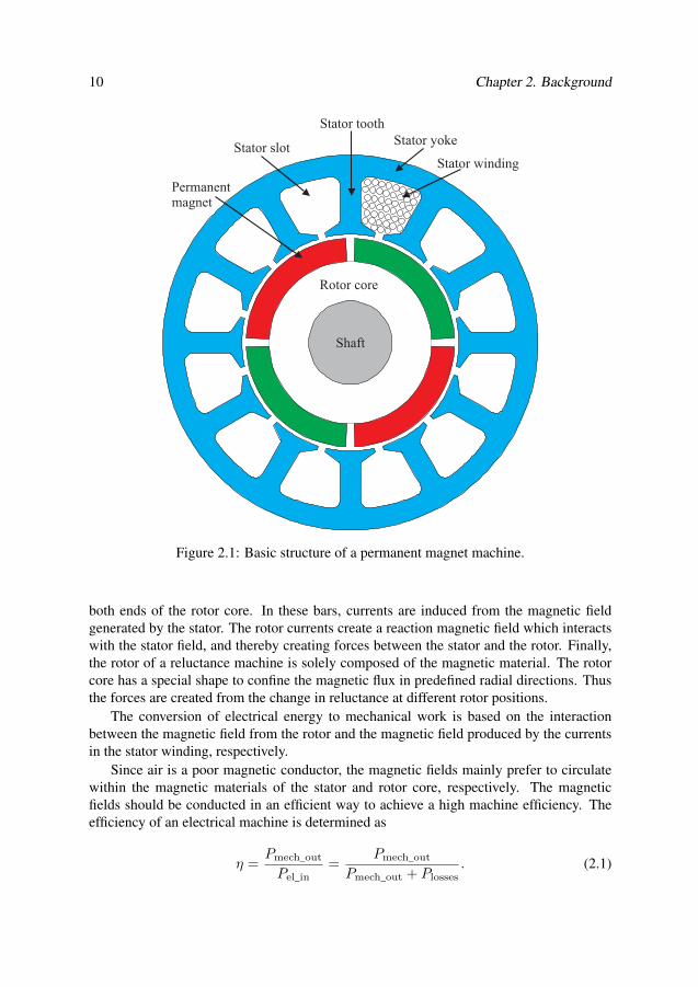
The basic structure of a typical electrical machine is shown in figure 2.1. It consists of afixed stator part and a moving rotor part. Generally speaking, the stator is built by the sameprinciple for all AC machines. It has a copper winding for conducting alternating electricalcurrents which, in turn, creates a rotating magnetic field. The winding is embedded inthe stator core, a structure composed of the stator yoke and the stator teeth. Both areusually made of a magnetic material confining the magnetic flux. However, since mostmagnetic materials are also good electrical conductors, the stator core is usually not builtas a single solid core, but stacked together with thin (0.1 mm to 1 mm) lamination sheets.These lamination sheets have a very thin (some µm) insulation layer to prevent currentsflowing in the axial direction of the core.
For AC machines, the rotor core is typically also made of laminated magnetic materials.However, synchronous machines offer the possibility to have a solid rotor core if the statorwindings create a sinusoidally distributed rotating flux. The major difference betweenmachine types (synchronous machine, permanent magnet machine, induction machine,and reluctance machine) is related to the magnetic field creation in the rotor. Synchronousmachines have a winding on the rotor which is fed from a DC power source to the rotorover brushes and slip rings. In permanent magnet motors, the magnetic field from the rotoris created by permanent magnets, mounted on the surface or inside the rotor core. The rotorof an induction machine consists of copper or aluminium bars which are short-circuited at
9
10 Chapter 2. Background
Stator yoke
Stator windingStator slot
Stator tooth
Permanentmagnet
Rotor core
Shaft
Figure 2.1: Basic structure of a permanent magnet machine.
both ends of the rotor core. In these bars, currents are induced from the magnetic fieldgenerated by the stator. The rotor currents create a reaction magnetic field which interactswith the stator field, and thereby creating forces between the stator and the rotor. Finally,the rotor of a reluctance machine is solely composed of the magnetic material. The rotorcore has a special shape to confine the magnetic flux in predefined radial directions. Thusthe forces are created from the change in reluctance at different rotor positions.
The conversion of electrical energy to mechanical work is based on the interactionbetween the magnetic field from the rotor and the magnetic field produced by the currentsin the stator winding, respectively.
Since air is a poor magnetic conductor, the magnetic fields mainly prefer to circulatewithin the magnetic materials of the stator and rotor core, respectively. The magneticfields should be conducted in an efficient way to achieve a high machine efficiency. Theefficiency of an electrical machine is determined as
η =Pmech_out
Pel_in=
Pmech_out
Pmech_out + Plosses. (2.1)

2.2. Losses in Electrical Machines 11
The difference between the mechanical output power Pmech_out and the electrical inputpower Pel_in are the losses Plosses. These losses are depending on the machine size, struc-ture, type and other factors like magnetic material properties. Typical loss values for ma-chines of different types and sizes are shown in the pie charts in figure 2.2. It can be seenthat in slower and larger machines, the winding losses usually dominate. For increasingspeeds, mechanical losses due to friction and iron losses due to the fast changing magneticfields become the major loss component. Especially the iron losses are in all machine typesa non-negligible contributor and are therefore studied in great details in this thesis.
25%16%
59%
a)
4%62%
34%
b)
22%49%
29%
Mechanicallosses
Windinglosses
Ironlosses
c)
Figure 2.2: Typical efficiency and loss values of a a) 110 kW permanent magnet high-speedgenerator (51 000 rpm) [7], b) 11 kW induction machine (1470 rpm) [8], c) 1 kW slot-lesspermanent magnet motor for hand tools (36 000 rpm).
2.2 Losses in Electrical Machines
There are several ways to improve the efficiency and to reduce losses in electrical ma-chines. In general, the losses in electrical machines can be separated into mechanicallosses, winding losses, and iron losses as shown in figure 2.3. The following sectionsdescribe these different loss components in more detail.
Losses in electrical machines
Mechanical losses
Friction losses Windage losses
Winding losses Iron losses
Figure 2.3: General loss separation in electrical machines.

12 Chapter 2. Background
2.2.1 Mechanical Losses
The major part of the mechanical losses in an electrical machine are the friction losses inthe bearings and the windage losses of the moving machine parts in gases or liquids.
The most common used bearings in electrical machines are ball bearings, but cylindri-cal roller bearings are also used frequently [9]. For normal operating conditions, a simpleestimation model of the frictional moment in rolling bearings is proposed by the bearingmanufacturer SKF [9]:
Mfr = 0.5µfrFbearingDbearing (2.2)
In (2.2), Fbearing is the equivalent dynamic bearing load in N, Dbearing the bearing borediameter in m, and µfr is the coefficient of friction. Table 2.1 gives an overview of thefriction coefficient µfr for different bearing types. The friction losses Pbearing in bearings
Table 2.1: Friction coefficient µfr for some rolling bearings used in electrical machines(selected data from [10]).
Bearing typeCoefficient of
friction µfr
Deep groove ball bearings 0.0015
Angular contact ball bearings
– single row 0.0020
– double row 0.0024– four-point contact 0.0024
Self-aligning ball bearings 0.0010
Cylindrical roller bearings
– with a cage 0.0011
– full complement 0.0020
Tapered roller bearings 0.0018
Cylindrical roller thrust bearings 0.0050
Spherical roller thrust bearings 0.0018
are consequently considered to increase proportional with the speed and can be determinedby
Pbearing = ωmMfr = ωm0.5µfrFbearingDbearing, (2.3)
where ωm is the mechanical angular frequency determined from the rotating speed n (inrpm) by
ωm =2πn
60. (2.4)
2.2. Losses in Electrical Machines 13
Since this thesis is focusing on electromagnetic losses in electrical machines, the readeris referred to relevant literature like [11] and [9] for further information on bearing lossesin electrical machines.
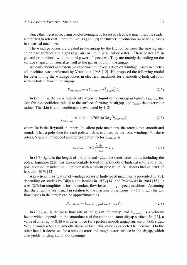
The windage losses are created in the airgap by the friction between the moving ma-chine part surfaces and a gas (e.g. air) or liquid (e.g. oil or water). These losses are ingeneral proportional with the third power of speed n3. They are mainly depending on thesurface shape and material as well as the gas or liquid in the airgap.
An early model and extensive experimental investigation on windage losses in electri-cal machines was performed by Vrancik in 1968 [12]. He proposed the following modelfor determining the windage losses in electrical machines for a smooth cylindrical rotorwith turbulent flow in the airgap:
Pwindage = πkfrictionγr4rotorω
3mlm (2.5)
In (2.5), γ is the mass density of the gas or liquid in the airgap in kg/m3, kfriction theskin friction coefficient related to the surfaces forming the airgap, and rrotor the outer rotorradius. The skin friction coefficient is evaluated by [12]
1
kfriction= 2.04 + 1.768 ln(Re
√
kfriction), (2.6)
where Re is the Reynolds number. In salient pole machines, the rotor is not smooth andround. It has a pole shoe for each pole which is enclosed by the rotor winding. For theserotors, Vrancik introduced another correction factor ksalient as
ksalient = 8.5lpole
rrotor+ 2.2. (2.7)
In (2.7), lpole is the length of the pole and rrotor the outer rotor radius including thepoles. Equation (2.5) was experimentally tested for a smooth cylindrical rotor and a fourpole homopolar induction alternator with a salient pole rotor. All results had an error ofless than 10 % [12].
A practical investigation of windage losses in high-speed machines is presented in [13],depending on studies by Bilgen and Boulos in 1973 [14] and Polkowski in 1984 [15]. Ituses (2.5) but simplifies it for the coolant flow losses in high-speed machines. Assumingthat the airgap is very small in relation to the machine dimensions (δ << rrotor) the gasflow losses in the airgap can be approximated as
Pwindage = kvelocityqm(ωmrrotor)2. (2.8)
In (2.8), qm is the mass flow rate of the gas in the airgap, and kvelocity is a velocityfactor which depends on the smoothness of the rotor and stator airgap surface. In [13], avalue of kvelocity = 0.48 was determined for a perfect smooth airgap surface on both sides.With a rough rotor and smooth stator surface, this value is expected to increase. On theother hand, it decreases for a smooth rotor and rough stator surface in the airgap, whichalso yields for deep stator slot openings.

14 Chapter 2. Background
Shaft mounted fans, often mounted on the non-drive end of the machine, can increasethe windage losses significantly. However, next to the rotational speed, the losses aredepending heavily on the exact shape and dimensions of the fan blades. Therefore, it isto the author’s knowledge not possible to give analytical equations for estimating thesefan windage losses. The loss values are generally determined either by computational fluiddynamics (CFD) simulations or by empirical equations and curve fittings based on previousloss measurements.
2.2.2 Winding Losses
The winding losses in electrical machines (often also called copper, ohmic, or resistivelosses) are the losses created by the current in the windings of the machine. The basicestimation is done by
Pcu = RphaseI2MΦ, (2.9)
where Rphase is the resistance of one phase winding and I the RMS value of the current inthe winding. MΦ is the number of phases of the machine. The resistance of each phase isdetermined by the geometry of the winding and the number of turns N as
Rphase =lcondNρ
Acond. (2.10)
In (2.10), lcond is the conductor length for one turn of the winding and Acond the cross-sectional area of the conductor. It has to be noted that the resistivity is changing withthe temperature. For general commercial copper used in electrical machine windings, theresistivity is ρcu20 = 1.75 × 10⁻⁸ Ωm at 20 C and its temperature coefficient is αcu =3.81 × 10⁻³ 1/K [16]. The resistivity of copper as a function of the temperature ϑ (in C)is then determined by
ρcu(ϑ) = ρcu20[1 + αcu(ϑ − 20 C)] (2.11)
Furthermore, depending on the conductor area and frequency, the skin-effect and proximityeffect have to be taken into account. A detailed description for calculations of these effectscan be found in [16], [17], and [18].
2.2.3 Iron Losses
The iron losses in the magnetic parts of the machine are also referred to as core losses ormagnetic losses. They are created by the changing magnetic field in the stator and rotormachine cores, respectively.
For conducting ferromagnetic materials, the iron losses are often separated into hys-teresis losses and eddy current losses. The former describes the losses due to the hysteresisproperties of the magnetic material. If a magnetic material is first slowly magnetized withan increasing magnetic field H and afterwards demagnetized with an opposing magnetic
2.2. Losses in Electrical Machines 15
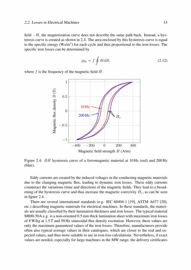
field −H , the magnetization curve does not describe the same path back. Instead, a hys-teresis curve is created as shown in 2.4. The area enclosed by this hysteresis curve is equalto the specific energy (Ws/m3) for each cycle and thus proportional to the iron losses. Thespecific iron losses can be determined by
pFe = f
∮
HdB, (2.12)
where f is the frequency of the magnetic field H .
−400 −200 0 200 400
−1
−0.5
0
0.5
1
Hc
10 Hz
200 Hz
Magnetic field strength H (A/m)
Mag
neti
cfl
uxde
nsit
yB
(T)
Figure 2.4: BH hysteresis curve of a ferromagnetic material at 10 Hz (red) and 200 Hz(blue).
Eddy currents are created by the induced voltages in the conducting magnetic materialsdue to the changing magnetic flux, leading to dynamic iron losses. These eddy currentscounteract the variations (time and direction) of the magnetic fields. They lead to a broad-ening of the hysteresis curve and thus increase the magnetic coercivity Hc, as can be seenin figure 2.4.
There are several international standards (e.g. IEC 60404-1 [19], ASTM A677 [20],etc.) describing magnetic materials for electrical machines. In these standards, the materi-als are usually classified by their lamination thickness and iron losses. The typical materialM800-50A e.g. is a non-oriented 0.5 mm thick lamination sheet with maximum iron lossesof 8 W/kg at 1.5 T and 50 Hz sinusoidal flux density excitation. However, these values areonly the maximum guaranteed values of the iron losses. Therefore, manufacturers provideoften also typical average values in their catalogues, which are closer to the real and ex-pected values, and thus more suitable to use in iron loss calculations. Nevertheless, if exactvalues are needed, especially for large machines in the MW range, the delivery certificates
16 Chapter 2. Background
for the lamination rolls provided from tests by the manufacturer are the best source for reli-able data. However, the manufacturing process of the magnetic machine parts is usually themain reason for discrepancies between the data sheet values and measurement results ofthe final assembled machine. So called “build factors” [21], “design factors” [22], or “losscorrection factors” [23] are commonly used to achieve better agreements between simu-lations and experimental results. These factors can be as large as 1.5 to 2 or even higherfor small machines [16]. This means that errors between the simulation and measurementresults of more than 50 % are not uncommon. Therefore, the effects of these influencingfactors are analysed and discussed in more detail in chapter 3.
The challenging point about determining the value of iron losses is that it is not pos-sible to measure them directly. Indirect thermal measurements (inverse thermal modelsand calorimetric measurements), magnetic field measurements (search coil windings, hallsensors, etc.) or loss separation calculations (subtracting all known other losses form thetotal losses) are the applied possibilities to determine indirectly iron losses in ferromag-netic materials for electrical machines. Chapter 6 gives an introduction and more detaileddescription about iron loss measurements.
2.3 Improvement Possibilities for Electrical Machines
To improve the efficiency of electrical machines, any of the previously discussed mechan-ical losses, the winding losses, and the iron losses have to be reduced. In general, higherefficiency is obtained by using better materials and/or more material. Improved bearingsand smoother airgap surfaces can reduce the mechanical losses. They are in general wellunderstood in electrical machines and are relatively easy to measure and calculate, if com-pared to electric and magnetic losses.
Better winding technologies (e.g. pre-pressed aluminium windings [24]) can increasethe electrical conducting area of the winding in the slots (increased slot fill factor). En-hanced cooling possibilities (e.g. inside the slots) reduce the ohmic resistance of the wind-ing itself. Both factors are reducing the winding losses and can be calculated, includingskin-effect and proximity effect, with high accuracy in machine models and with FEMsoftware.
The iron losses in the stator and rotor core can be reduced by using better and thinnerlamination sheet materials and improving manufacturing processes to decrease the mag-netic material property deterioration in the stator and rotor core. Eddy current losses in-crease e.g. proportional with the square of the lamination sheet thickness. Thus, thinnerlamination sheets are typically used in high-speed machines.
For applications with increasing speed and run by power electronics inverters withvarying switching frequencies, iron losses can become the dominant loss contributor. High-speed machines and machines with large field weakening capabilities are such cases (seefigure 2.2).
2.4. Conclusions 17
2.4 Conclusions
First, the basic concept of energy conversion in electrical machines was introduced. After-wards, a classification of losses in electrical machines was discussed. General loss calcu-lation methods were presented briefly, including theory and calculation methods for deter-mining mechanical losses, winding losses and iron losses in electrical machines. The mainfocus of this work are the iron losses, which generally are also the most complicated lossesto predict in electrical machines. Therefore, they are investigated and discussed in moredetail in the next chapters.

Chapter 3
Iron Losses in Electrical Machines
Even though iron losses in electrical machines have been investigated for more than 100
years, there is still a significant discrepancy between iron loss prediction and measurement
results. The sources for the discrepancies are, on the one hand, the difficulty to measure
and determine the iron losses in the final assembled machine correctly. On the other hand,
modelling the physical processes and effects behind the iron losses is a difficult challenge.
The lack of accuracy of the models developed so far is the other source for the used factors.
This chapter gives a short introduction on experimental and analytical iron loss determi-
nation methods. Iron loss influencing factors due to the machine manufacturing process
are described and analysed.
3.1 Iron Loss Determination
There is no physical way to measure and determine the iron losses in magnetic materialsdirectly. International IEC and ASTM standards describe measurement methods to deter-mine iron losses in special shaped lamination sheets with an Epstein frame [25][26][27]or by ring shaped probes (ring specimen measurements) [28]. These measurements useelectrical windings to create magnetic fields in and around the investigated material. Themagnetic flux density in the material can then be determined with a secondary winding, inwhich a certain voltage is induced by the changing magnetic field in the materials. Ironlosses are then calculated from the magnetic field H and the flux density B inside thematerial. The determined iron losses from these measurements can then later be used asmaterial input parameters for calculating iron losses in electrical machines with the helpof FEM simulations or analytical equations. A detailed description of available magneticmeasurement methods is given in chapter 6.1.
Models predicting iron losses require inputs in form of measurement results and tech-nical data of the used electrical steels. The needed data is depending on the used iron lossmodel. Considering two identical machines made from the same electrical sheets cataloguetype but different manufacturers, the iron losses vary in reality due to non-isotropic effects,different alloy composites, contamination, and deterioration during the manufacturing pro-
19
20 Chapter 3. Iron Losses in Electrical Machines
cess [29]. The latter is discussed in section 3.2.Procedures for examining iron losses in assembled electrical machines are described in
international IEC and IEEE standards [30], [31]. General loss measurements are conductedfor several operating points of the machines, including no-load tests, load tests and short-circuit tests. Iron losses are then determined as the “other losses”. They are the left overafter subtracting the winding losses and the mechanical losses from the total losses ofthe machine. Hence, all errors in the determination of input power, output power, ohmicwinding losses or mechanical losses directly add up in an error in the iron loss values.Nevertheless, this method is still the state of the art in determining iron losses due to itssimplicity, ease of implementation and fast results.
An approach to determine iron losses locally in an electrical machine is possible bylocal thermal measurements. At a local point, losses can be determined directly from thechange of temperature at this point. A requirement is that the heat flow around this point isnegligible small compared to the occurring losses and that all surrounding areas have thesame initial steady state condition. The method is often referred to as the inverse thermalmodel (ITM). Chapter 11 describes this method in more details, where its implementationand limitations for an outer-rotor permanent magnet synchronous machine are presented.
Next to the correct experimental determination of iron losses, the modelling of ironlosses is the other key factor for accurately identifying iron losses in electrical machines.Charles Proteus Steinmetz proposed the first mathematical approach to determine ironlosses in magnetic materials in 1884 [32]. Today, around 130 years later, scientists aroundthe world are still proposing new models and methods to determine and simulate iron lossesunder arbitrary conditions in electromagnetic devices more accurately. Improvements ofthe original Steinmetz equation are still used for modelling iron losses in electrical ma-chines. However, most recent publications use the iron loss separation model approach(often called the Bertotti model) which divides the iron losses into hysteresis losses, eddycurrent losses, and sometimes also excess losses. More advanced iron loss models try todescribe the physical hysteresis characteristics of the materials mathematically. However,these models need more input parameters and require longer calculation times. Therefore,it is a trade-off between the investigated efforts and the needed accuracy of the results. Anexhaustive list and a detailed description of these iron loss models are presented in chapter4.
It should be kept in mind that the engineering approach of iron loss separation into dif-ferent loss types (hysteresis losses and eddy current losses in example) and related modelsrepresents an empirical approach which tries to separate the different physical influencesdue to frequency and flux density variations in electromagnetic systems into different com-ponents. However, it does not explain the real physical phenomena of the iron lossesdirectly. From a physical point of view, both the hysteresis losses and the eddy currentlosses in the conducting ferromagnetic materials, are based on Joule heating [33]. Theyare caused by the same physical phenomena: every change in magnetization (which alsooccurs at DC magnetization) is a movement of magnetic domain walls and creates (mi-croscopic and macroscopic) eddy currents which, in turn, create Joule heating. The factthat hysteresis losses also arise at almost zero frequency is due to the fact that even ifthe macroscopic magnetization change is very slow, the local magnetization inside the do-

3.2. Iron Loss Influencing Factors 21
mains is changing rapidly and discrete in time, which generates eddy current losses [33].Nevertheless, the loss separation shows in most cases good correlation with measurementsand has therefore its justification in the engineering science. It should be added that ironlosses due to spin relaxation are negligible for electrical machines. Their impact is onlynoticeable at frequencies in the MHz range and above [34].
3.2 Iron Loss Influencing Factors
The different production steps of electrical machine stator cores influence the iron lossessignificantly. However, the degree of magnetic property degradation is heavily dependingon the tools and stator core handling during the manufacturing process. Figure 3.1 providesan overview on typical influencing factors during the manufacturing process of electricalmachine cores. The full deterioration effects on the material due to the cutting and as-sembling manufacturing step together are investigated for an electrical permanent magnetmachine with a non-oriented electrical steel stator core in [35]. A posteriori estimations ofthe manufacturing process effects in induction machines by measurements are presentedin [36]. The following subsections describe the three manufacturing steps in more details.
Influencing Factors
Cutting
PunchingLaser
cutting
Electricaldischargemachining
Stacking
Welding Glueing Interlocking
Housingassembly
Heatshrinking
Formfitting
Figure 3.1: Influencing factors of the manufacturing process of electrical machine cores.
3.2.1 Punching and Cutting
Cutting and punching the iron sheets influence the material properties and create inhomo-geneous stress inside the sheets. The stress, in turn, influences the hysteresis curve byshearing. The effect is depending on the alloy composite. The grain size in the sheetsseems to be the main influencing factor for typical non-oriented electrical steels, especiallyfor operating ranges between 0.4 T to 1.5 T [37], [38]. The influenced region in the sheetdue to cutting and punching can go up to 10 mm in distance from the cut edge, where thepermeability is significantly decreased [39], [40]. This reduction in permeability increasesthe iron losses in the material. Especially for geometric parts smaller than 10 mm in width(thin stator teeth for example), the punching process can have a significant influence on
22 Chapter 3. Iron Losses in Electrical Machines
the iron losses. Therefore, in these cases, punching has to be considered in the loss calcu-lation [41]. An approach to determine the damaged area of punched lamination sheets ispresented in [42].
Different cutting technologies as punching, laser cutting, and electrical discharge ma-chining deteriorate the magnetic properties in different ways. Punching introduces mainlya mechanical deformation stress at the cut edge, whereas laser cutting and discharge ma-chining introduce a thermal stress in the cut edge due to a very high and fast local heatingand melting processes.
A formula for estimating the iron losses in the teeth of induction machines is developedin [43]. Ways to determine and regard the cut edge influences in design tools are presentedin [44], [45]. For considering the effect of the punching area in FEM machine simulations,an approach using an empirical degradation profile is proposed in 3.2. It should be men-tioned that the width of the electric sheets for standard loss measurements in the Epsteinframe is 30 mm and thus not suitable for material and loss investigations of small sheetparts.
An important aspect to consider is that it is possible to recover the magnetic materialcharacteristics up to a certain degree by a stress-relieving heat treatment, called annealing,after the process of machining [39], [46]. This annealing process is mainly applied to ma-chines with small geometrical measurements where the cut edges account for a significantpart of the geometry, or large high efficient machines where the iron loss reduction is a keyfactor. Since the annealing process changes also the hardness and mechanical strengthsof some materials, it is depending on the used cutting technology and the material if theannealing is more effective before or after the cutting process [47]. The cutting and punch-ing process damages the thin insulation layer which can lead to short circuits betweenseveral sheet layers. Additional losses due to eddy currents circulating axially in severallaminations will occur.
3.2.2 Stacking and Welding
Similar deterioration as for cutting and punching effects is obtained due to the stackingand welding process during the machine core assembly. The axial pressure applied duringglueing and welding the lamination sheets of the core introduces mechanical stress and,thus, deteriorates the magnetic material properties. The welding process introduces alsothermal stress locally at the welding seams which influences the magnetic properties of thematerial depending on the seam width and its thickness. Furthermore, the welding processdestroys the insulation layers between the lamination sheets due to the local heating andcreates short circuits between the sheets by the welding seams. These short circuit pathsbetween the lamination sheets increase the eddy current losses as part of the total ironlosses in the core [48]–[50]. To reduce the impact of the welding seams, they are usuallycreated on the outer stator yoke surface where the magnetic flux density has its lowestvalue in the stator yoke. Finally, the significance of the stacking and welding impact forSiFe is more pronounced for high-Si content alloys compared to low-Si content ones [49].
3.3. Conclusions 23
3.2.3 Final Assembly Step
Pressing the stator core into its frame in the last manufacturing step can create significantstresses in the whole stator yoke structure. Especially for the heat shrinking process, wherethe machine housing is first heated up to expand before the stator core is pressed intothe housing, the radial pressure and thus the induced stresses can be severe and lead tosignificant increased iron losses [50]. But also the normal press fitting and stator corefixation by glueing or screws introduce stress which has a negative impact on the ironlosses [49]. It should be noted that the effect of the housing assembly step is more evidentfor better quality lamination sheets with higher Si content and can even negate the usuallybetter magnetic properties of the material [50].
3.3 Conclusions
A detailed analysis of iron losses from a historic perspective and present research trendswere presented in this chapter. Challenges regarding the iron loss determination and ironloss model groups were discussed briefly. An overview of the manufacturing process ef-fects on the iron losses in electrical machines was given.
An exhaustive classification and description of iron loss models is given in the nextchapter. The influencing factors during the manufacturing process are also investigated inmore detail in section 5.3.

Chapter 4
Iron Loss Models for Electrical
Machines
To predict the iron losses during the design or optimization process of electrical machines,
engineers can choose from a wide range of models. This chapter discusses the development
of these iron loss models in more detail and compares them in terms of possible flux density
waveforms (i.e. time variations), rotating field consideration, needed material data, and
accuracy.
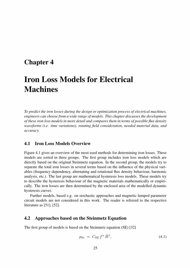
4.1 Iron Loss Models Overview
Figure 4.1 gives an overview of the most used methods for determining iron losses. Thesemodels are sorted in three groups. The first group includes iron loss models which aredirectly based on the original Steinmetz equation. In the second group, the models try toseparate the total iron losses in several terms based on the influence of the physical vari-ables (frequency dependency, alternating and rotational flux density behaviour, harmonicanalysis, etc.). The last group are mathematical hysteresis loss models. These models tryto describe the hysteresis behaviour of the magnetic materials mathematically or empiri-cally. The iron losses are then determined by the enclosed area of the modelled dynamichysteresis curves.
Further models, based e.g. on stochastic approaches and magnetic lumped parametercircuit models are not considered in this work. The reader is referred to the respectiveliterature as [51], [52].
4.2 Approaches based on the Steinmetz Equation
The first group of models is based on the Steinmetz equation (SE) [32]
pFe = CSE fα Bβ , (4.1)
25

26 Chapter 4. Iron Loss Models for Electrical Machines
Iron
loss
calc
ula
tion
mod
els
Ste
inm
etz
base
dm
odel
s
Mod
ified
Ste
inm
etz
(MS
E)
Gen
eral
ized
Ste
inm
etz
(GS
E)
Impr
oved
Gen
eral
ized
Ste
inm
etz
(iG
SE
)
Nat
ural
Ste
inm
etz
(NS
E)
Los
sse
para
tion
(hys
tere
sis
&ed
dycu
rren
ts)
Ano
mal
ous
fact
orC
lass
ical
and
dyna
mic
eddy
curr
ent
sepa
rati
on
Rot
atio
nal
corr
ecti
onfa
ctor
Mat
hem
atic
alhy
ster
esis
mod
els
Cla
ssic
alP
reis
ach
mod
el
Dyn
amic
Pre
isac
hm
odel
Los
ssu
rfac
em
odel
(LS
M)
Vis
cosi
ty-
base
dm
agne
tody
nam
icm
odel
Fri
ctio
nli
kehy
ster
esis
mod
el
Jile
s/A
ther
ton
mod
el
Ope
rahy
ster
esis
mod
el
Figure 4.1: Model approaches to determine iron losses in electrical machines.
4.2. Approaches based on the Steinmetz Equation 27
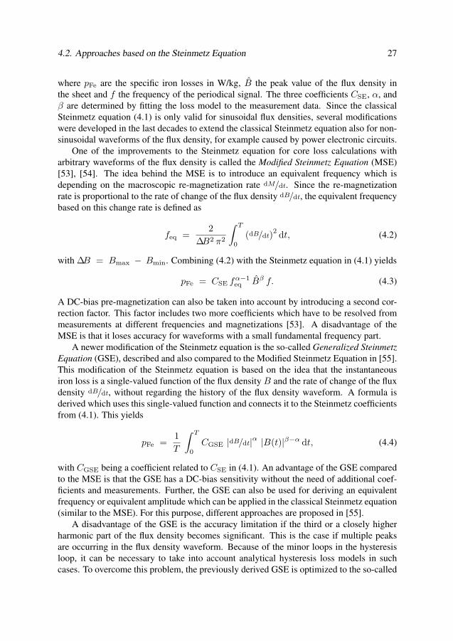
where pFe are the specific iron losses in W/kg, B the peak value of the flux density inthe sheet and f the frequency of the periodical signal. The three coefficients CSE, α, andβ are determined by fitting the loss model to the measurement data. Since the classicalSteinmetz equation (4.1) is only valid for sinusoidal flux densities, several modificationswere developed in the last decades to extend the classical Steinmetz equation also for non-sinusoidal waveforms of the flux density, for example caused by power electronic circuits.
One of the improvements to the Steinmetz equation for core loss calculations witharbitrary waveforms of the flux density is called the Modified Steinmetz Equation (MSE)[53], [54]. The idea behind the MSE is to introduce an equivalent frequency which isdepending on the macroscopic re-magnetization rate dM/dt. Since the re-magnetizationrate is proportional to the rate of change of the flux density dB/dt, the equivalent frequencybased on this change rate is defined as
feq =2
∆B2 π2
∫ T
0
(dB/dt)2
dt, (4.2)
with ∆B = Bmax − Bmin. Combining (4.2) with the Steinmetz equation in (4.1) yields
pFe = CSE fα−1eq Bβ f. (4.3)
A DC-bias pre-magnetization can also be taken into account by introducing a second cor-rection factor. This factor includes two more coefficients which have to be resolved frommeasurements at different frequencies and magnetizations [53]. A disadvantage of theMSE is that it loses accuracy for waveforms with a small fundamental frequency part.
A newer modification of the Steinmetz equation is the so-called Generalized Steinmetz
Equation (GSE), described and also compared to the Modified Steinmetz Equation in [55].This modification of the Steinmetz equation is based on the idea that the instantaneousiron loss is a single-valued function of the flux density B and the rate of change of the fluxdensity dB/dt, without regarding the history of the flux density waveform. A formula isderived which uses this single-valued function and connects it to the Steinmetz coefficientsfrom (4.1). This yields
pFe =1
T
∫ T
0
CGSE |dB/dt|α
|B(t)|β−α dt, (4.4)
with CGSE being a coefficient related to CSE in (4.1). An advantage of the GSE comparedto the MSE is that the GSE has a DC-bias sensitivity without the need of additional coef-ficients and measurements. Further, the GSE can also be used for deriving an equivalentfrequency or equivalent amplitude which can be applied in the classical Steinmetz equation(similar to the MSE). For this purpose, different approaches are proposed in [55].
A disadvantage of the GSE is the accuracy limitation if the third or a closely higherharmonic part of the flux density becomes significant. This is the case if multiple peaksare occurring in the flux density waveform. Because of the minor loops in the hysteresisloop, it can be necessary to take into account analytical hysteresis loss models in suchcases. To overcome this problem, the previously derived GSE is optimized to the so-called
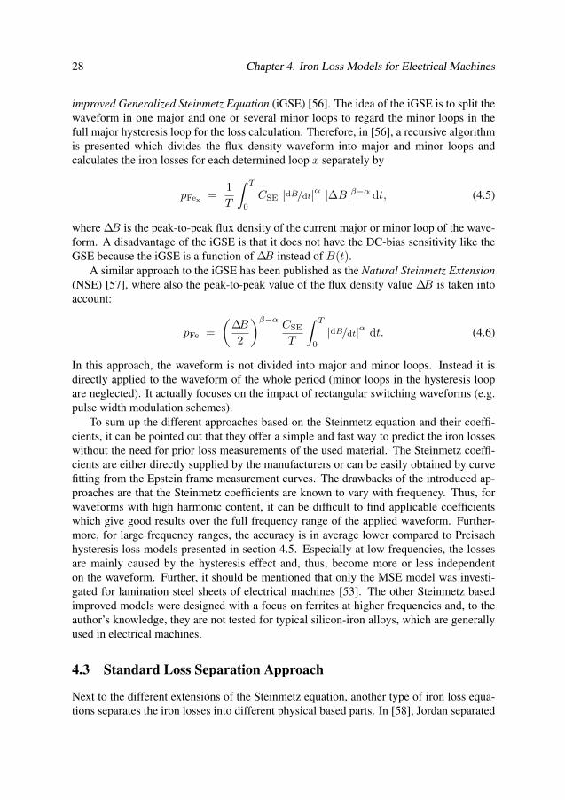
28 Chapter 4. Iron Loss Models for Electrical Machines
improved Generalized Steinmetz Equation (iGSE) [56]. The idea of the iGSE is to split thewaveform in one major and one or several minor loops to regard the minor loops in thefull major hysteresis loop for the loss calculation. Therefore, in [56], a recursive algorithmis presented which divides the flux density waveform into major and minor loops andcalculates the iron losses for each determined loop x separately by
pFex=
1
T
∫ T
0
CSE |dB/dt|α
|∆B|β−α dt, (4.5)
where ∆B is the peak-to-peak flux density of the current major or minor loop of the wave-form. A disadvantage of the iGSE is that it does not have the DC-bias sensitivity like theGSE because the iGSE is a function of ∆B instead of B(t).
A similar approach to the iGSE has been published as the Natural Steinmetz Extension
(NSE) [57], where also the peak-to-peak value of the flux density value ∆B is taken intoaccount:
pFe =
(
∆B
2
)β−αCSE
T
∫ T
0
|dB/dt|α
dt. (4.6)
In this approach, the waveform is not divided into major and minor loops. Instead it isdirectly applied to the waveform of the whole period (minor loops in the hysteresis loopare neglected). It actually focuses on the impact of rectangular switching waveforms (e.g.pulse width modulation schemes).
To sum up the different approaches based on the Steinmetz equation and their coeffi-cients, it can be pointed out that they offer a simple and fast way to predict the iron losseswithout the need for prior loss measurements of the used material. The Steinmetz coeffi-cients are either directly supplied by the manufacturers or can be easily obtained by curvefitting from the Epstein frame measurement curves. The drawbacks of the introduced ap-proaches are that the Steinmetz coefficients are known to vary with frequency. Thus, forwaveforms with high harmonic content, it can be difficult to find applicable coefficientswhich give good results over the full frequency range of the applied waveform. Further-more, for large frequency ranges, the accuracy is in average lower compared to Preisachhysteresis loss models presented in section 4.5. Especially at low frequencies, the lossesare mainly caused by the hysteresis effect and, thus, become more or less independenton the waveform. Further, it should be mentioned that only the MSE model was investi-gated for lamination steel sheets of electrical machines [53]. The other Steinmetz basedimproved models were designed with a focus on ferrites at higher frequencies and, to theauthor’s knowledge, they are not tested for typical silicon-iron alloys, which are generallyused in electrical machines.
4.3 Standard Loss Separation Approach
Next to the different extensions of the Steinmetz equation, another type of iron loss equa-tions separates the iron losses into different physical based parts. In [58], Jordan separated

4.3. Standard Loss Separation Approach 29
the losses depending on the relationship of the variation to the frequency (f and f2) andon the amplitude of the flux density (B2). This means the losses are separated into (static)hysteresis losses and (dynamic) eddy current losses:
pFe = physt + pec = ChystfB2 + Cecf2B2. (4.7)
In (4.7), Chyst and Cec are the hysteresis and eddy current coefficient, respectively. InJordan’s approach, it is assumed that the hysteresis losses are proportional to the hysteresisloop area of the material at low frequencies (f → 0 Hz). The eddy current part of thelosses pec can be approximated from Maxwell’s equations. This leads to
pec =d2(dB(t)/dt)
2
12 ρ γ, (4.8)
where B(t) is the flux density as a function of time, d the lamination sheet thickness, and ρand γ the specific resistivity and the material density of the lamination sheets, respectively.Equation (4.7) has been proven correct for several nickel-iron alloys but lacks accuracyfor silicon-iron alloys [59]. For this reason, an empirical correction factor ηexc, called theexcess loss factor (often also referred to as anomalous loss factor), was introduced by Pryand Bean [60]. It extends (4.7) to
pFe = physt + ηa pec =
Chyst f B2 + ηexc Cec f2 B2, (4.9)
with ηexc = pec_measured
pec_calculated> 1. For thin grain oriented silicon-iron alloys, ηexc reaches
values between 2 and 3 [59].Another approach to improve (4.7) is to introduce an additional loss term pexc to take
into account the excess losses as a function of the flux density and frequency. It separatesthe iron loss formula pFe into three terms, the static hysteresis losses physt, dynamic eddycurrent losses pec, and the excess losses pexc:
pFe = physt + pec + pexc =
Chyst f B2 + Cec f2 B2 + Cexc f1.5 B1.5. (4.10)
Since the excess losses in (4.10) are still based on empirical factors, Bertotti developed atheory, leading to a statistical model to calculate the iron losses by introducing so-calledmagnetic objects, which led to a physical description and function of the loss factor Cexc
in terms of the active magnetic objects and the domain wall motion [61]–[64]:
Cexc =√
S V0 σ G. (4.11)
In (4.11), S is the cross sectional area of the lamination sample, G≈0.136 a dimensionlesscoefficient of the eddy current damping, and σ the electric conductivity of the laminationsheets. V0 characterizes the statistical distribution of the local coercive fields and takes intoaccount the grain size [63]. In recent studies, it was observed that the hysteresis losses of
30 Chapter 4. Iron Loss Models for Electrical Machines
highly alloyed silicon iron lamination sheets and other alloys do not really fit the first termin (4.10) regarding the flux density squared dependency. Thus, another fitting coefficient αis introduced, which is usually between 1.6 and 2.2 for ferromagnetic materials and alloys.Including this factor leads to the following equation which is nowadays also often usedin the post processing calculations of finite element software, either with α = 2 [65] or avariable α [66], [67]:
pFe = Chyst f Bα + Cec f2 B2 + Cexc f1.5 B1.5. (4.12)
It has to be noted that the presented loss separation approaches does not hold if the skineffect is not negligible [68]. A recent study on the properties of the coefficients fromBertotti’s statistical model is presented in [69].
4.4 Rotational Iron Loss Models
It has to be mentioned that the magnetic fields are assumed to be alternating in the previouspresented models. This is typically the case in electrical transformers. However, in electri-cal machines, the flux in the stator is rotating with time. Several approaches, focusing onthe iron losses due to a rotational magnetization in the sheets (also called rotational losses),are introduced in [70]–[74]. A review on rotational iron loss measurement methods andmodels can be found in [75] and [76], and an international comparison and measurementstudy on rotating iron losses is presented in [77].
The iron losses in electrical machines caused by rotational magnetization occur mainlyin the tooth heads/tips and in the intersection areas between the teeth and the yoke. In thegenerally largest part of the machine, i.e. in the middle of the teeth and in the middle ofthe yoke, the magnetization is mainly unidirectional.
An equivalent approach to the loss separation model in (4.10) was chosen for rota-tional losses and it was shown that rotational losses show a similar non-linear behaviouras alternating iron losses [78]. It is further shown in the same article that the ratio of therotating losses to the alternating losses (prot/palt) decreases monotonically with increasingflux density B.
An often applied practical approach for iron losses in electrical machines is the sep-aration model after the magnetizing processes. This means that the losses caused by analternating magnetization, a rotational magnetization and higher harmonics are added upto determine the total iron losses in the machine [79]:
pFe = C1 pa + C2 prot + C3 phf . (4.13)
In (4.13), pa are the losses caused by alternating magnetization, prot the losses caused byrotational magnetization and phf the losses caused by higher harmonics. Cx are empiricalmaterial and geometric dependent factors from measurements and curve fittings. They canalso take into account manufacturing correction factors [79].
Another possibility to investigate iron losses due to rotational magnetization is by in-troducing a further correction factor in the two term loss separation model in (4.7). This is

4.5. Hysteresis Models 31
done in [80], where a rotational loss factor due to rotational magnetization is added to theeddy current loss term.
pFe = a2 B2 f + (a1 + a4 Ba3)B2 f2. (4.14)
In (4.14), a1 =Cec anda2 = Chyst(1+ Bmin
Bmax(r−1)), with r the rotational hysteresis factor
and Bmin and Bmax the minimum and maximum values of B(t) over one period. Theterm a4 and the exponent a3 are used to get an accurate representation of the iron losses atlarge fields by introducing a higher order of the flux density B. Thus, they are called highorder loss factors. Further, a3 is depending on the lamination thickness. The excess lossterm Cexc is negligible compared to the other terms in this model and thus not regarded in(4.14).
4.5 Hysteresis Models
To obtain a higher accuracy of the iron loss prediction, mathematical hysteresis models canbe used if measurements of full hysteresis curves of the investigated material or even moreparameters are available. Next to the well documented classical hysteresis models fromPreisach [81], [82] and Jiles/Atherton [83], there are several improved and modified ironloss models applicable to steel sheets and complete electrical machines proposed in theliterature. Generally, they require more measurements and material data of the electricalsteel sheets compared to the simpler Steinmetz and loss separation models. However,they also give better results in terms of accuracy at the cost of more complex simulations.Furthermore, it is also possible to regard minor-loops and DC pre-magnetization by usingmodifications of these models (e.g. in [84]). The iron losses can be calculated with thesemodels by determining the area of the full BH hysteresis loop with
pFe =1
T
∫ T
0
H dB. (4.15)
Some applicable improved and modified hysteresis models are amongst others the dy-namic Preisach model [82], the loss surface model [85], the viscosity-based magnetody-namic model [86], the friction like hysteresis model [87], and the Opera hysteresis model[88]. They are discussed in more detail in the following subsections. Since the first fourmentioned hysteresis models are based on or related to the classical Preisach model, a shortintroduction to the Preisach model is given below.
4.5.1 Classical Preisach Hysteresis Model
The classical Preisach model was first published in 1935 by the German physicist FranzPreisach [81]. The discrete model is based on a number n of simple rectangular hysteresisloops (also called relays) and weight functions w, as it is shown in the block diagram in fig-ure 4.2. The rectangular hysteresis loops are represented by a hysteresis operators Rαn,βn
,which are connected in parallel and multiplied by a weight function w (also called Preisach
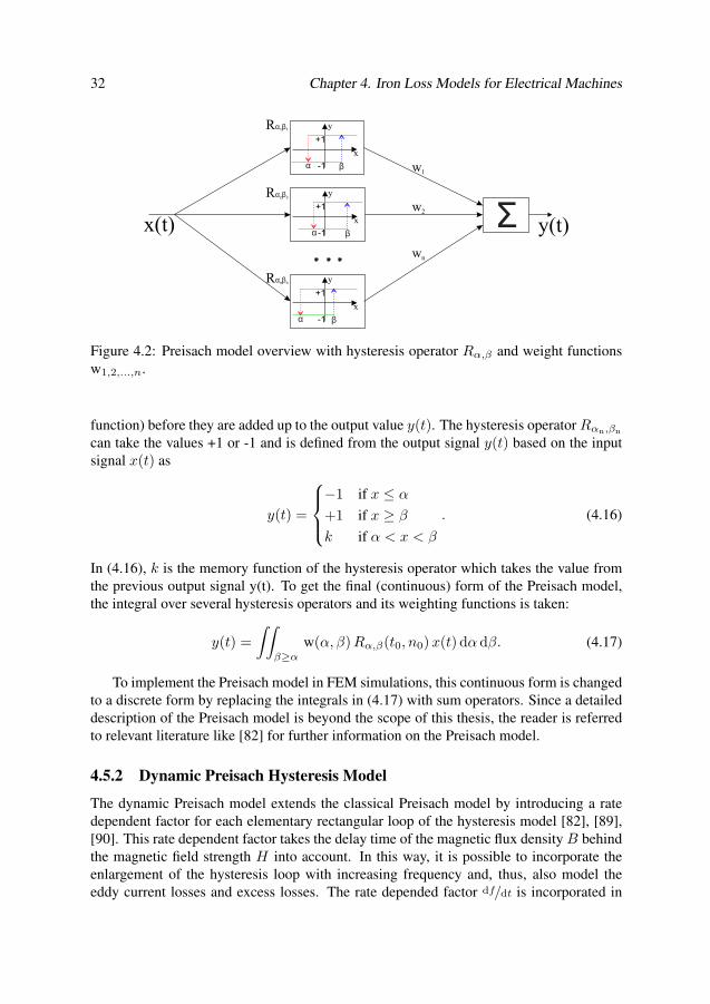
32 Chapter 4. Iron Loss Models for Electrical Machines
+1
-1
x
y
α β
x(t) y(t)
R 1 1α β
R 2 2α β
R n nα β
w1
w2
wn
Σ+1
-1
x
y
α β
+1
-1
x
y
α β
Figure 4.2: Preisach model overview with hysteresis operator Rα,β and weight functionsw1,2,...,n.
function) before they are added up to the output value y(t). The hysteresis operator Rαn,βn
can take the values +1 or -1 and is defined from the output signal y(t) based on the inputsignal x(t) as
y(t) =
−1 if x ≤ α
+1 if x ≥ β
k if α < x < β
. (4.16)
In (4.16), k is the memory function of the hysteresis operator which takes the value fromthe previous output signal y(t). To get the final (continuous) form of the Preisach model,the integral over several hysteresis operators and its weighting functions is taken:
y(t) =
∫∫
β≥α
w(α, β) Rα,β(t0, n0) x(t) dα dβ. (4.17)
To implement the Preisach model in FEM simulations, this continuous form is changedto a discrete form by replacing the integrals in (4.17) with sum operators. Since a detaileddescription of the Preisach model is beyond the scope of this thesis, the reader is referredto relevant literature like [82] for further information on the Preisach model.
4.5.2 Dynamic Preisach Hysteresis Model
The dynamic Preisach model extends the classical Preisach model by introducing a ratedependent factor for each elementary rectangular loop of the hysteresis model [82], [89],[90]. This rate dependent factor takes the delay time of the magnetic flux density B behindthe magnetic field strength H into account. In this way, it is possible to incorporate theenlargement of the hysteresis loop with increasing frequency and, thus, also model theeddy current losses and excess losses. The rate depended factor df/dt is incorporated in
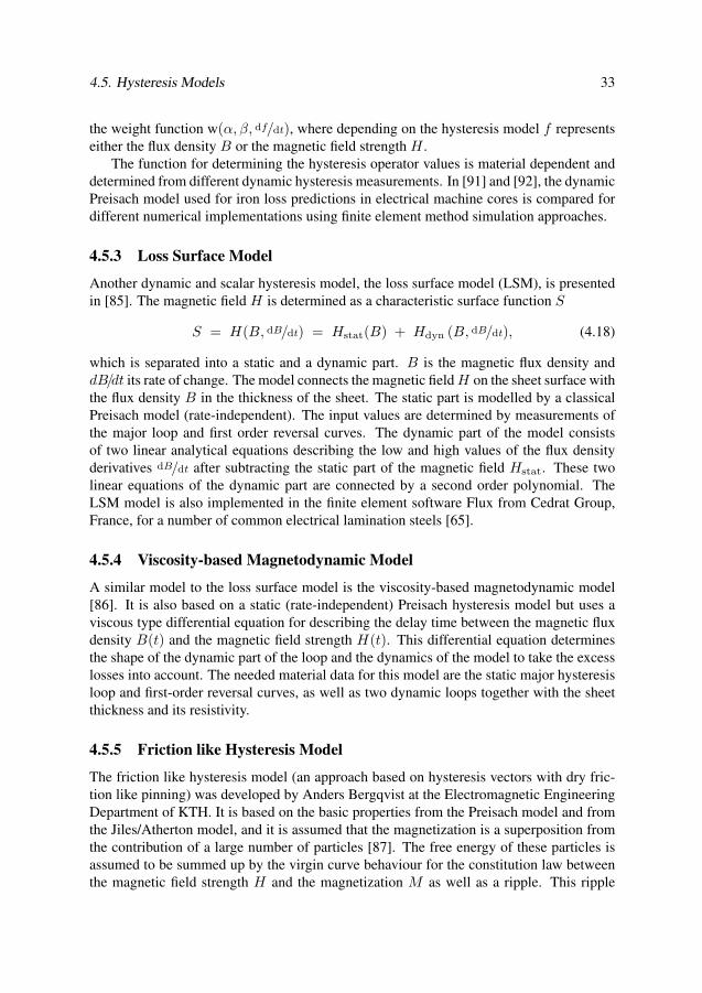
4.5. Hysteresis Models 33
the weight function w(α, β, df/dt), where depending on the hysteresis model f representseither the flux density B or the magnetic field strength H .
The function for determining the hysteresis operator values is material dependent anddetermined from different dynamic hysteresis measurements. In [91] and [92], the dynamicPreisach model used for iron loss predictions in electrical machine cores is compared fordifferent numerical implementations using finite element method simulation approaches.
4.5.3 Loss Surface Model
Another dynamic and scalar hysteresis model, the loss surface model (LSM), is presentedin [85]. The magnetic field H is determined as a characteristic surface function S
S = H(B, dB/dt) = Hstat(B) + Hdyn (B, dB/dt), (4.18)
which is separated into a static and a dynamic part. B is the magnetic flux density anddB/dt its rate of change. The model connects the magnetic field H on the sheet surface withthe flux density B in the thickness of the sheet. The static part is modelled by a classicalPreisach model (rate-independent). The input values are determined by measurements ofthe major loop and first order reversal curves. The dynamic part of the model consistsof two linear analytical equations describing the low and high values of the flux densityderivatives dB/dt after subtracting the static part of the magnetic field Hstat. These twolinear equations of the dynamic part are connected by a second order polynomial. TheLSM model is also implemented in the finite element software Flux from Cedrat Group,France, for a number of common electrical lamination steels [65].
4.5.4 Viscosity-based Magnetodynamic Model
A similar model to the loss surface model is the viscosity-based magnetodynamic model[86]. It is also based on a static (rate-independent) Preisach hysteresis model but uses aviscous type differential equation for describing the delay time between the magnetic fluxdensity B(t) and the magnetic field strength H(t). This differential equation determinesthe shape of the dynamic part of the loop and the dynamics of the model to take the excesslosses into account. The needed material data for this model are the static major hysteresisloop and first-order reversal curves, as well as two dynamic loops together with the sheetthickness and its resistivity.
4.5.5 Friction like Hysteresis Model
The friction like hysteresis model (an approach based on hysteresis vectors with dry fric-tion like pinning) was developed by Anders Bergqvist at the Electromagnetic EngineeringDepartment of KTH. It is based on the basic properties from the Preisach model and fromthe Jiles/Atherton model, and it is assumed that the magnetization is a superposition fromthe contribution of a large number of particles [87]. The free energy of these particles isassumed to be summed up by the virgin curve behaviour for the constitution law betweenthe magnetic field strength H and the magnetization M as well as a ripple. This ripple
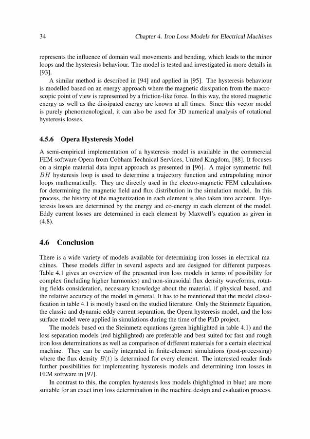
34 Chapter 4. Iron Loss Models for Electrical Machines
represents the influence of domain wall movements and bending, which leads to the minorloops and the hysteresis behaviour. The model is tested and investigated in more details in[93].
A similar method is described in [94] and applied in [95]. The hysteresis behaviouris modelled based on an energy approach where the magnetic dissipation from the macro-scopic point of view is represented by a friction-like force. In this way, the stored magneticenergy as well as the dissipated energy are known at all times. Since this vector modelis purely phenomenological, it can also be used for 3D numerical analysis of rotationalhysteresis losses.
4.5.6 Opera Hysteresis Model
A semi-empirical implementation of a hysteresis model is available in the commercialFEM software Opera from Cobham Technical Services, United Kingdom, [88]. It focuseson a simple material data input approach as presented in [96]. A major symmetric fullBH hysteresis loop is used to determine a trajectory function and extrapolating minorloops mathematically. They are directly used in the electro-magnetic FEM calculationsfor determining the magnetic field and flux distribution in the simulation model. In thisprocess, the history of the magnetization in each element is also taken into account. Hys-teresis losses are determined by the energy and co-energy in each element of the model.Eddy current losses are determined in each element by Maxwell’s equation as given in(4.8).
4.6 Conclusion
There is a wide variety of models available for determining iron losses in electrical ma-chines. These models differ in several aspects and are designed for different purposes.Table 4.1 gives an overview of the presented iron loss models in terms of possibility forcomplex (including higher harmonics) and non-sinusoidal flux density waveforms, rotat-ing fields consideration, necessary knowledge about the material, if physical based, andthe relative accuracy of the model in general. It has to be mentioned that the model classi-fication in table 4.1 is mostly based on the studied literature. Only the Steinmetz Equation,the classic and dynamic eddy current separation, the Opera hysteresis model, and the losssurface model were applied in simulations during the time of the PhD project.
The models based on the Steinmetz equations (green highlighted in table 4.1) and theloss separation models (red highlighted) are preferable and best suited for fast and roughiron loss determinations as well as comparison of different materials for a certain electricalmachine. They can be easily integrated in finite-element simulations (post-processing)where the flux density B(t) is determined for every element. The interested reader findsfurther possibilities for implementing hysteresis models and determining iron losses inFEM software in [97].
In contrast to this, the complex hysteresis loss models (highlighted in blue) are moresuitable for an exact iron loss determination in the machine design and evaluation process.

4.6. Conclusion 35
These models need much more knowledge about the material data or prior material mea-surements as well as more information about the flux density waveforms in the machine.Furthermore, the integration into finite-element software is more complicated (especiallyif it is part of the solving process), but the results have generally also a higher accuracy.
What all models have in common is the challenge to identify the correct parameters ofthe considered material. Depending on the complexity of the model, more or less extensiveiron loss measurements are needed for identifying the correct model parameters. As dis-cussed in section 3.2, a significant change during the manufacturing process was pointedout as a main reason for the discrepancies between simulated and measured iron losses inelectrical machines. Therefore, it is important to consider the material degradation in thedetermination of the iron loss model parameters, as will be shown in later chapters of thisthesis.
So far, the iron losses have been described mainly from the point of view of electricalmachine experts. They cover only slightly the real physical phenomena of iron lossesand focus instead on a black-box approach. Iron losses are experimentally determined bymeasurements and iron loss models fitted mathematically to the observed input and outputsignals. The next chapter takes a closer look at the complex mechanisms in magneticmaterials exposed to external magnetic fields and explains why a black-box approach isused by engineers, even though the results might be less accurate.
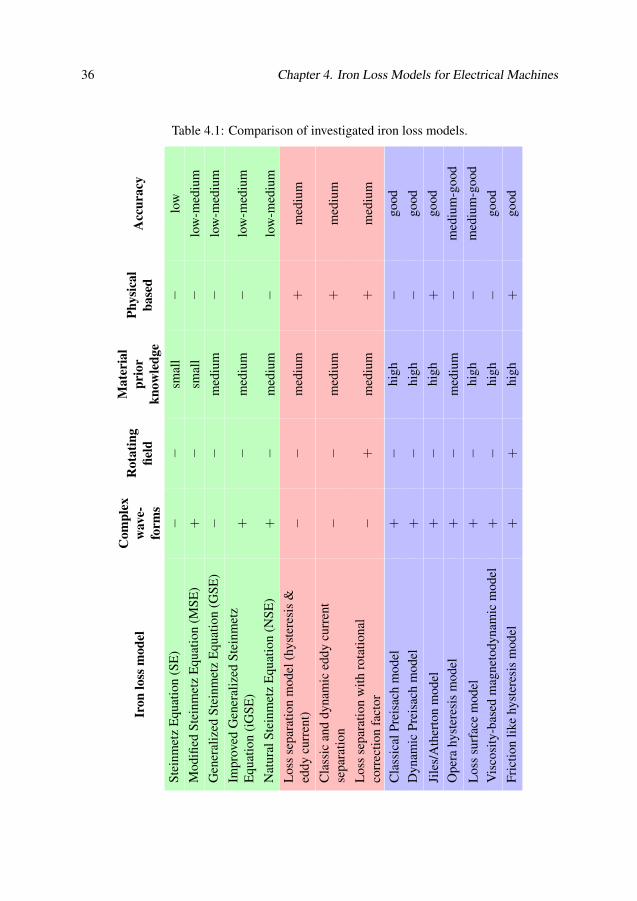
36 Chapter 4. Iron Loss Models for Electrical Machines
Table 4.1: Comparison of investigated iron loss models.Ir
on
loss
mod
el
Com
ple
x
wave-
form
s
Rota
tin
g
fiel
d
Mate
rial
pri
or
kn
ow
led
ge
Ph
ysi
cal
base
dA
ccu
racy
Ste
inm
etz
Equ
atio
n(S
E)
−−
smal
l−
low
Mod
ified
Ste
inm
etz
Equ
atio
n(M
SE
)+
−sm
all
−lo
w-m
ediu
m
Gen
eral
ized
Ste
inm
etz
Equ
atio
n(G
SE
)−
−m
ediu
m−
low
-med
ium
Impr
oved
Gen
eral
ized
Ste
inm
etz
Equ
atio
n(i
GS
E)
+−
med
ium
−lo
w-m
ediu
m
Nat
ural
Ste
inm
etz
Equ
atio
n(N
SE
)+
−m
ediu
m−
low
-med
ium
Los
sse
para
tion
mod
el(h
yste
resi
s&
eddy
curr
ent)
−−
med
ium
+m
ediu
m
Cla
ssic
and
dyna
mic
eddy
curr
ent
sepa
rati
on−
−m
ediu
m+
med
ium
Los
sse
para
tion
wit
hro
tati
onal
corr
ecti
onfa
ctor
−+
med
ium
+m
ediu
m
Cla
ssic
alP
reis
ach
mod
el+
−hi
gh−
good
Dyn
amic
Pre
isac
hm
odel
+−
high
−go
od
Jile
s/A
ther
ton
mod
el+
−hi
gh+
good
Ope
rahy
ster
esis
mod
el+
−m
ediu
m−
med
ium
-goo
d
Los
ssu
rfac
em
odel
+−
high
−m
ediu
m-g
ood
Vis
cosi
ty-b
ased
mag
neto
dyna
mic
mod
el+
−hi
gh−
good
Fri
ctio
nli
kehy
ster
esis
mod
el+
+hi
gh+
good
Chapter 5
Magnetic Materials for Electrical
Machines
In this chapter, typical magnetic materials for electrical machines are introduced. The
phenomena in the material which occur under the magnetization process by external fields
are described. Several materials are outlined and their physical characteristics are com-
pared. A loss-to-squared-flux-density factor is defined to give electrical machine designers
a tool for selecting the most suitable material for a certain machine application from the
manufacturer data-sheet information.
5.1 Introduction to Magnetic Materials and Magnetization
From the physical point of view, there exist only three materials which present the propertyof magnetic conduction at general machine operation temperatures. These three materialsare iron (Fe), nickel (Ni) and cobalt (Co). They are classified as ferromagnetic materialsand are the strongest type of materials in magnetism.
Pure cobalt can reach saturation polarisations Js of 1.79 T, has a Curie temperature of1125 C, and has excellent magnetic properties [34]. However, it is very soft in its purestate and also the most expensive material among the three. Nickel lies from the point ofcost in between cobalt and iron. It has in its pure state the lowest saturation polarisation of0.6 T and the lowest Curie temperature of 360 C among these three materials [34]. On theother hand, nickel has the highest relative permeability µr with values up to 50 × 103 andmore. This leads to a very low field coercivity and thus to the lowest hysteresis losses forferromagnetic materials. Pure iron is by far the cheapest material of the three. It can reachflux densities of 2.15 T and has a Curie temperature of 770 C [34]. But in its pure state,it has also the highest electrical conductivity, leading to the largest losses, especially withincreasing frequency.
From a magnetic point of view, all ferromagnetic materials consist of many so calledWeiss domains which have a size of 10−1 to 10 × 10−3 mm3. Each domain consists ofabout 106 to 109 atoms. These domains are separated by domain walls (in ferromagnetic
37
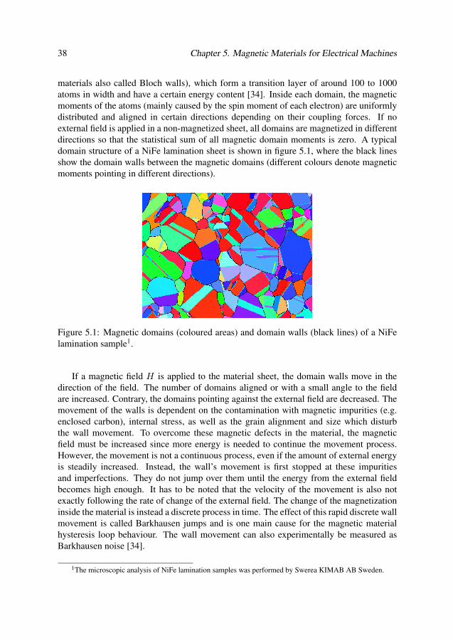
38 Chapter 5. Magnetic Materials for Electrical Machines
materials also called Bloch walls), which form a transition layer of around 100 to 1000atoms in width and have a certain energy content [34]. Inside each domain, the magneticmoments of the atoms (mainly caused by the spin moment of each electron) are uniformlydistributed and aligned in certain directions depending on their coupling forces. If noexternal field is applied in a non-magnetized sheet, all domains are magnetized in differentdirections so that the statistical sum of all magnetic domain moments is zero. A typicaldomain structure of a NiFe lamination sheet is shown in figure 5.1, where the black linesshow the domain walls between the magnetic domains (different colours denote magneticmoments pointing in different directions).
Figure 5.1: Magnetic domains (coloured areas) and domain walls (black lines) of a NiFelamination sample1.
If a magnetic field H is applied to the material sheet, the domain walls move in thedirection of the field. The number of domains aligned or with a small angle to the fieldare increased. Contrary, the domains pointing against the external field are decreased. Themovement of the walls is dependent on the contamination with magnetic impurities (e.g.enclosed carbon), internal stress, as well as the grain alignment and size which disturbthe wall movement. To overcome these magnetic defects in the material, the magneticfield must be increased since more energy is needed to continue the movement process.However, the movement is not a continuous process, even if the amount of external energyis steadily increased. Instead, the wall’s movement is first stopped at these impuritiesand imperfections. They do not jump over them until the energy from the external fieldbecomes high enough. It has to be noted that the velocity of the movement is also notexactly following the rate of change of the external field. The change of the magnetizationinside the material is instead a discrete process in time. The effect of this rapid discrete wallmovement is called Barkhausen jumps and is one main cause for the magnetic materialhysteresis loop behaviour. The wall movement can also experimentally be measured asBarkhausen noise [34].
1The microscopic analysis of NiFe lamination samples was performed by Swerea KIMAB AB Sweden.
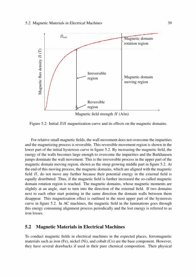
5.2. Magnetic Materials in Electrical Machines 39
Reversibleregion
Irreversibleregion Magnetic domain
moving region
Magnetic domainrotation region
Bsat
Magnetic field strength H (A/m)
Mag
neti
cfl
uxde
nsit
yB
(T)
Figure 5.2: Initial BH magnetization curve and its effects on the magnetic domains.
For relative small magnetic fields, the wall movement does not overcome the impuritiesand the magnetizing process is reversible. This reversible movement region is shown in thelower part of the initial hysteresis curve in figure 5.2. By increasing the magnetic field, theenergy of the walls becomes large enough to overcome the impurities and the Barkhausenjumps dominate the wall movement. This is the irreversible process in the upper part of themagnetic domain moving region, shown as the steep growing middle part in figure 5.2. Atthe end of this moving process, the magnetic domains, which are aligned with the magneticfield H , do not move any further because their potential energy in the external field isequally distributed. Thus, if the magnetic field is further increased the so-called magneticdomain rotation region is reached. The magnetic domains, whose magnetic moments areslightly at an angle, start to turn into the direction of the external field. If two domainsnext to each other start pointing in the same direction the domain walls between themdisappear. This magnetization effect is outlined in the most upper part of the hysteresiscurve in figure 5.2. In AC machines, the magnetic field in the laminations goes throughthis energy consuming alignment process periodically and the lost energy is referred to asiron losses.
5.2 Magnetic Materials in Electrical Machines
To conduct magnetic fields in electrical machines in the expected places, ferromagneticmaterials such as iron (Fe), nickel (Ni), and cobalt (Co) are the base component. However,they have several drawbacks if used in their pure chemical composition. Their physical
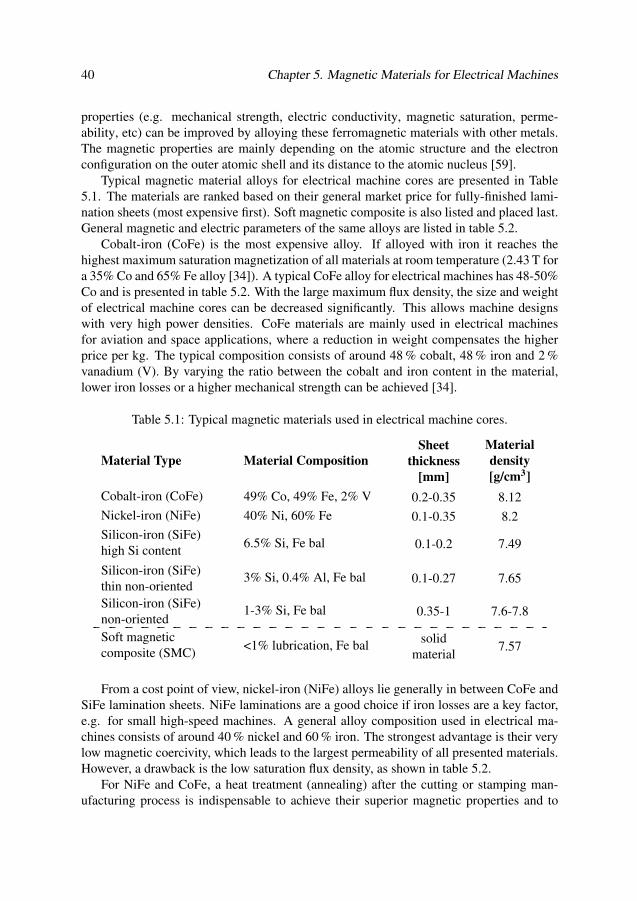
40 Chapter 5. Magnetic Materials for Electrical Machines
properties (e.g. mechanical strength, electric conductivity, magnetic saturation, perme-ability, etc) can be improved by alloying these ferromagnetic materials with other metals.The magnetic properties are mainly depending on the atomic structure and the electronconfiguration on the outer atomic shell and its distance to the atomic nucleus [59].
Typical magnetic material alloys for electrical machine cores are presented in Table5.1. The materials are ranked based on their general market price for fully-finished lami-nation sheets (most expensive first). Soft magnetic composite is also listed and placed last.General magnetic and electric parameters of the same alloys are listed in table 5.2.
Cobalt-iron (CoFe) is the most expensive alloy. If alloyed with iron it reaches thehighest maximum saturation magnetization of all materials at room temperature (2.43 T fora 35% Co and 65% Fe alloy [34]). A typical CoFe alloy for electrical machines has 48-50%Co and is presented in table 5.2. With the large maximum flux density, the size and weightof electrical machine cores can be decreased significantly. This allows machine designswith very high power densities. CoFe materials are mainly used in electrical machinesfor aviation and space applications, where a reduction in weight compensates the higherprice per kg. The typical composition consists of around 48 % cobalt, 48 % iron and 2 %vanadium (V). By varying the ratio between the cobalt and iron content in the material,lower iron losses or a higher mechanical strength can be achieved [34].
Table 5.1: Typical magnetic materials used in electrical machine cores.
Material Type Material Composition
Sheet
thickness
[mm]
Material
density
[g/cm3]
Cobalt-iron (CoFe) 49% Co, 49% Fe, 2% V 0.2-0.35 8.12
Nickel-iron (NiFe) 40% Ni, 60% Fe 0.1-0.35 8.2
Silicon-iron (SiFe)high Si content
6.5% Si, Fe bal 0.1-0.2 7.49
Silicon-iron (SiFe)thin non-oriented
3% Si, 0.4% Al, Fe bal 0.1-0.27 7.65
Silicon-iron (SiFe)non-oriented
1-3% Si, Fe bal 0.35-1 7.6-7.8
Soft magneticcomposite (SMC)
<1% lubrication, Fe balsolid
material7.57
From a cost point of view, nickel-iron (NiFe) alloys lie generally in between CoFe andSiFe lamination sheets. NiFe laminations are a good choice if iron losses are a key factor,e.g. for small high-speed machines. A general alloy composition used in electrical ma-chines consists of around 40 % nickel and 60 % iron. The strongest advantage is their verylow magnetic coercivity, which leads to the largest permeability of all presented materials.However, a drawback is the low saturation flux density, as shown in table 5.2.
For NiFe and CoFe, a heat treatment (annealing) after the cutting or stamping man-ufacturing process is indispensable to achieve their superior magnetic properties and to

5.2. Magnetic Materials in Electrical Machines 41
Table 5.2: Magnetic and electric properties of typical magnetic materials used in electricalmachine cores. B8 and B25 are measured at H = 800 A/m and H = 2500 A/m.
Material Type B8 [T] B25 [T]Resistivity
[µΩcm]
Cobalt-iron (CoFe) 2.1 2.23 40
Nickel-iron (NiFe) 1.44 1.48 60
Silicon-iron (SiFe)high Si content 1.29 1.4 82
Silicon-iron (SiFe)thin non-oriented
1.15 1.63 52
Silicon-iron (SiFe)non-oriented
1.64 20-60
Soft magneticcomposite (SMC) 0.71 1.22 20000
adjust the mechanical strength characteristics. Especially for CoFe, a trade off betweenoptimal magnetic and mechanical parameters has to be made during the annealing process.A higher annealing temperature leads generally to better magnetic properties at the costof lower mechanical strength and vice versa. A detailed study of the annealing processinfluence is presented in chapter 10.
The most widely used material in electrical machines nowadays is iron alloyed witha small amount of silicon (in general referred to as silicon-iron or SiFe laminations). Itis available in a grain-oriented state (i.e. the material is anisotropic and has a differentpermeability in different directions) or a non-oriented state (i.e. almost isotropic magneticproperties in all directions [98]). Electrical transformers usually use grain-oriented mag-netic materials due to their unidirectional flux change in the core. In contrast, electricalmachines mainly use non-oriented materials since the flux direction is generally not unidi-rectional but changes direction (it rotates in the stator yoke and tooth tips).
For non-oriented SiFe lamination sheets, the iron content varies between 93 % forhighly alloyed SiFe, and up to 99 % for low SiFe steels. The remaining content of SiFe isthen silicon (Si) with weight % contents up to 6.5 %, aluminium (Al) up to 1 %, and man-ganese (Mn) up to 0.5 %. The silicon makes the iron mechanically harder and increasesthe electrical resistivity. The downside is a slight decrease in the saturation magnetizationand smaller permeability [99]. Aluminium has a similar increasing effect on the electricalresistivity but also lowers the permeability of the material. A higher manganese contentleads to larger grains and thus a higher permeability, but increases the losses as well [100].
SiFe with a high silicon-content (up to 6.5 %) are mostly used for high-speed machinesdue to their large electrical resistivity and thus low eddy current losses. However, the Sicontent makes the alloy more brittle, resulting in more complicated and expensive man-ufacturing processes. Cheaper and capable of higher flux densities are the so called thinSiFe alloys. They have around 3 % of silicon content and, thus, a lower electrical resis-
42 Chapter 5. Magnetic Materials for Electrical Machines
tivity. However, the small lamination thickness still keeps the eddy current losses lowat the cost of larger assembly efforts and thus production costs compared to thicker non-oriented SiFe laminations. Both, high silicon content and thin SiFe laminations are mainlyused in small high-speed machines. The vast majority of industrial machines are man-ufactured with standard non-oriented SiFe laminations, having silicon contents of 0.5 %to 3 %. Sheet thicknesses of 0.5 mm or thicker keep the manufacturing costs lower andgive, in most cases, a sufficient performance in terms of efficiency and costs for generalindustrial machines.
Special attention has to be paid to soft magnetic composite (SMC) materials, whichconsist of a powder of very small isolated iron particles. Machine parts made of thismaterial are not produced as stacked lamination sheets but directly pressed together tosingle-part or multi-part machine cores. The advantage of the powder is the possibility forspecial machine geometries with three-dimensional flux paths. Furthermore, its very highresistivity leads to low eddy current losses which is a significant advantage for high-speedmachines. The downside is its relatively low permeability and flat BH magnetizationcurve, leading to relatively small maximum flux density values at typical magnetic fieldstrengths in electrical machines [101]. Further information about the compositions of SMCmaterials and possible future developments are described in [102].
5.3 Material Selection for Electrical Machines
Due to the saturation effect in ferromagnetic materials, electrical machines are generallydesigned to work just below the saturation knee point of the BH magnetization curve, asit is shown in figure 5.3. However, since the BH magnetization curve is different for eachlamination material, the machine geometry has to be adapted to have an efficient utilizationof the magnetic material in terms of ohmic winding losses (efficient current use) and thevolume and weight of the core (efficient iron use).
Material manufacturers provide in general typical magnetic and physical data of theirlamination steels. This data can be used for a rough first estimation and for comparing dif-ferent materials in terms of BH magnetization curves and iron loss densities for a certainmachine design. But it is difficult to evaluate both parameters at the same time. In order tohelp electrical machine designers to choose the best material for a certain machine design,a loss-to-squared-flux-density (PB2) factor is introduced. This factor is defined as the ironloss density (W/kg) over the flux density (T) squared. The idea behind this factor is that itdoes not vary much with the flux density, allowing a visual representation of its value inthe BH magnetization curve by filled circles of different sizes. A decreasing circle sizefor a given material with increasing values of B means that the specific iron losses aredepending on Bα, with α lower than 2. At a given value of a flux density and frequency, alarger circle represents a higher loss density. This allows for a visual comparison betweenmaterials and gives an objective material grading to select the most suitable material for acertain machine application in terms of magnetic saturation, material utilization and ironlosses.
Figure 5.4 gives a comparison of the initial BH magnetization curves for typical mate-

5.4. Conclusions 43
Inefficient iron use
Ideal working area
Inefficient current use
Magnetic field strength H (A/m)
Mag
neti
cfl
uxde
nsit
yB
(T)
Figure 5.3: Machine operating points on the initial hysteresis magnetization curve.
rials used in high-performance electrical machines, together with the PB2 factor at 50 Hzand 400 Hz. For 50 Hz, CoFe and NiFe, the two most expensive materials, are also thebest in terms of saturation magnetization (largest magnetic flux density) and iron losses(smallest circles), respectively. For larger frequencies (400 Hz), very thin and high alloyedSiFe (6.5% Si) has the lowest losses. However, machine designers should be aware thatthe magnetic materials in the manufactured motor may show quite different properties thanexpected due to the deterioration during the manufacturing process. This is due to the factthat the typical manufacturer data does not take stresses from cutting and welding or othermanufacturing steps into account. It should be added as well that different materials reactdifferently to each manufacturing step and other influences. Regarding the change in ironlosses due to the welding process for example, it is shown in section 7.2 that NiFe alloyshave a larger percentage loss increase due to the welding process than SiFe alloys.
An overview of the different manufacturing influencing factors on the iron losses andmagnetic properties for typical SiFe lamination sheets are given in Table 5.3. In this ta-ble, Physt denotes the hysteresis losses, Pec the classical eddy current losses and Pexc theexcess losses. Js and Hc are the saturation magnetization and the coercive field strength,respectively.
5.4 Conclusions
In this chapter, the magnetisation process of ferromagnetic materials used in electrical ma-chines was briefly introduced. The physical background behind the magnetization process,iron loss creation and external influencing factors were discussed. An overview of typi-cal ferromagnetic materials used in electrical machines for different application areas was
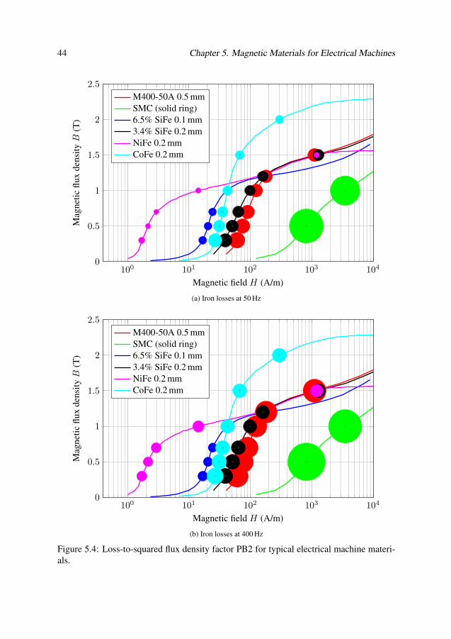
44 Chapter 5. Magnetic Materials for Electrical Machines
100 101 102 103 1040
0.5
1
1.5
2
2.5
Magnetic field H (A/m)
Mag
neti
cfl
uxde
nsit
yB
(T)
M400-50A 0.5 mmSMC (solid ring)6.5% SiFe 0.1 mm3.4% SiFe 0.2 mmNiFe 0.2 mmCoFe 0.2 mm
(a) Iron losses at 50 Hz
100 101 102 103 1040
0.5
1
1.5
2
2.5
Magnetic field H (A/m)
Mag
neti
cfl
uxde
nsit
yB
(T)
M400-50A 0.5 mmSMC (solid ring)6.5% SiFe 0.1 mm3.4% SiFe 0.2 mmNiFe 0.2 mmCoFe 0.2 mm
(b) Iron losses at 400 Hz
Figure 5.4: Loss-to-squared flux density factor PB2 for typical electrical machine materi-als.

5.4. Conclusions 45
Table 5.3: Influence of different physical and manufacturing factors on typical SiFe lami-nation sheet properties [45], [103], [104].
Influencing Factor P hyst P ec P exc J s Hc
Grain size (dgrain ր) ց ր ց
Impurities (ր) ր ց ր
Sheet thickness (d ր) ց ր ց
Internal stress (ր) ր ր
Cutting/punching process ր ց
Pressing process ր
Alloy content (%Si ր) ց ց
presented with general physical parameters and material characteristics.These magnetic data from the material manufacturers can be used to do a first compar-
ison between different materials. A tool to select the most suitable magnetic material for acertain electrical machine design was introduced. The loss-to-squared-flux-density (PB2)factor allows to compare the BH magnetisation curve and iron losses for typical electricalmachine alloys at the same time.
The next chapter presents how these material data are obtained according to interna-tional standards as well as the test bench developed during this project.

Chapter 6
Assessment and Evaluation of Magnetic
Materials for Electrical Machines
Most of the volume in classical electrical machines is occupied by magnetic materials con-
stituting an as good as possible magnetic path. In machines with planar flux paths (2D
geometries) the material is laminated to reduce eddy current losses in the core. To charac-
terize materials, different measurement methods are presented in this chapter. Afterwards,
the measurement system build up during this PhD project is explained in detail. The focus
on the measurement setup is on ring core specimen tests, but it is also possible to conduct
tests with an Epstein frame. More details about ring core specimen measurements are
presented in the last part of this chapter.
6.1 Introduction to Magnetic Measurements
There are different ways to investigate and evaluate the magnetic properties and iron lossesof lamination steel sheets. For focusing purely on the sheet material properties, and ne-glecting any machine geometry, Epstein frame measurements and single sheet tests areapplied. In these tests, the size and geometry of the test sample are determined by the stan-dard and are independent on the later application. These tests are preferably used to specifycatalogue values and to compare lamination sheets between different manufacturers. Ringcore measurements are used for evaluating small geometries (e.g. cutting effects), softmagnetic composite, and materials with large permeability values. The advantage of ringcores is a closed magnetic path without any airgaps. Furthermore, they can be applied tostator cores. The method was applied in the material investigations of small slot-less per-manent magnetic machines for industrial applications. This is described in more detail insection 6.3.
Figure 6.1 shows typical testing tools and objects for investigating magnetic materialproperties. A detailed description of these measurement setups is beyond the scope of thethesis. Further literature can be found in the corresponding standard for the Epstein frame[25]–[27] and single sheet testers [105], [106]. A full guide of magnetic measurements can
47
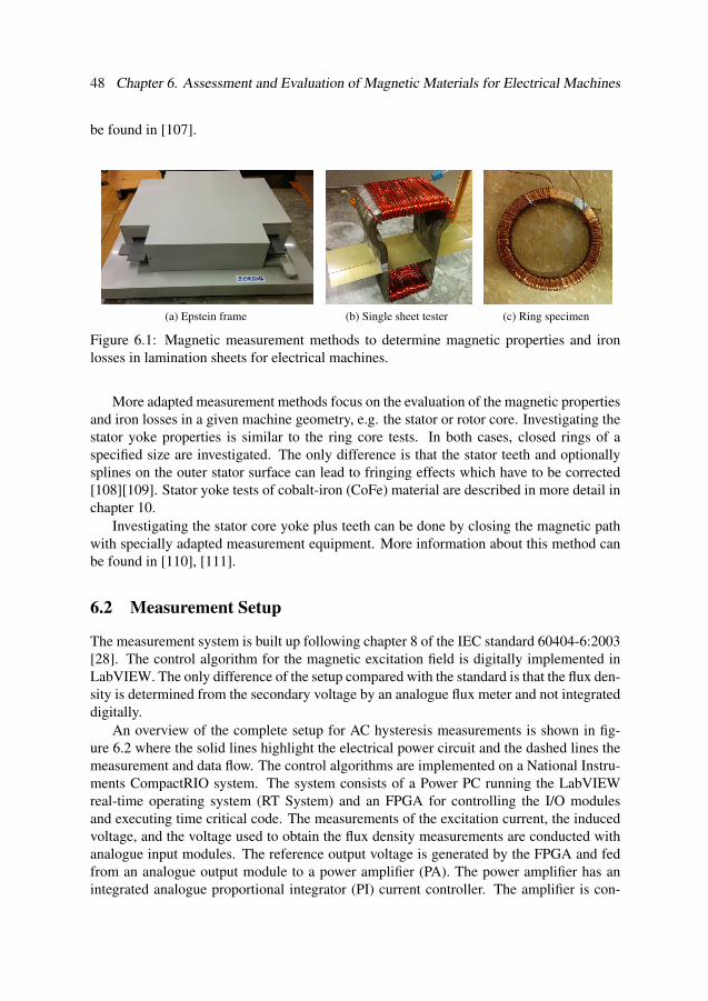
48 Chapter 6. Assessment and Evaluation of Magnetic Materials for Electrical Machines
be found in [107].
(a) Epstein frame (b) Single sheet tester (c) Ring specimen
Figure 6.1: Magnetic measurement methods to determine magnetic properties and ironlosses in lamination sheets for electrical machines.
More adapted measurement methods focus on the evaluation of the magnetic propertiesand iron losses in a given machine geometry, e.g. the stator or rotor core. Investigating thestator yoke properties is similar to the ring core tests. In both cases, closed rings of aspecified size are investigated. The only difference is that the stator teeth and optionallysplines on the outer stator surface can lead to fringing effects which have to be corrected[108][109]. Stator yoke tests of cobalt-iron (CoFe) material are described in more detail inchapter 10.
Investigating the stator core yoke plus teeth can be done by closing the magnetic pathwith specially adapted measurement equipment. More information about this method canbe found in [110], [111].
6.2 Measurement Setup
The measurement system is built up following chapter 8 of the IEC standard 60404-6:2003[28]. The control algorithm for the magnetic excitation field is digitally implemented inLabVIEW. The only difference of the setup compared with the standard is that the flux den-sity is determined from the secondary voltage by an analogue flux meter and not integrateddigitally.
An overview of the complete setup for AC hysteresis measurements is shown in fig-ure 6.2 where the solid lines highlight the electrical power circuit and the dashed lines themeasurement and data flow. The control algorithms are implemented on a National Instru-ments CompactRIO system. The system consists of a Power PC running the LabVIEWreal-time operating system (RT System) and an FPGA for controlling the I/O modulesand executing time critical code. The measurements of the excitation current, the inducedvoltage, and the voltage used to obtain the flux density measurements are conducted withanalogue input modules. The reference output voltage is generated by the FPGA and fedfrom an analogue output module to a power amplifier (PA). The power amplifier has anintegrated analogue proportional integrator (PI) current controller. The amplifier is con-
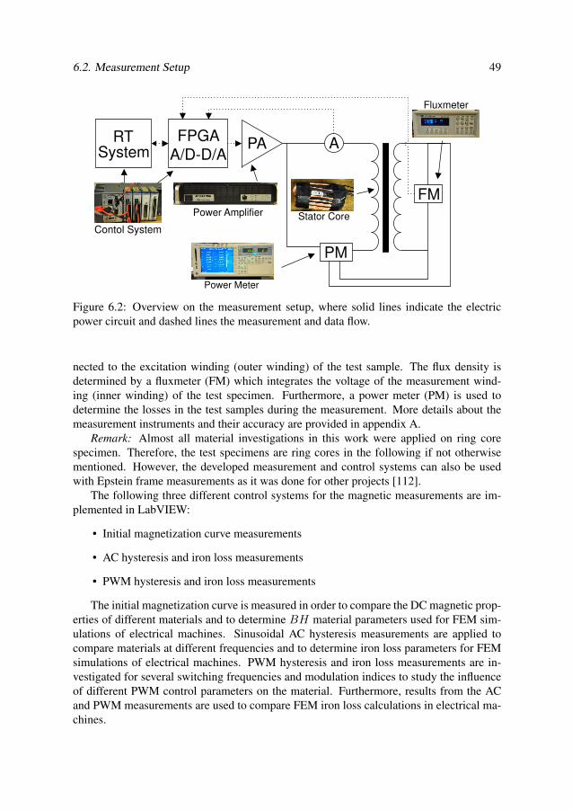
6.2. Measurement Setup 49
FPGA
A/D-D/AAPA
PM
Power Meter
Power Amplifier
RTSystem
FM
Fluxmeter
Contol System
Stator Core
Figure 6.2: Overview on the measurement setup, where solid lines indicate the electricpower circuit and dashed lines the measurement and data flow.
nected to the excitation winding (outer winding) of the test sample. The flux density isdetermined by a fluxmeter (FM) which integrates the voltage of the measurement wind-ing (inner winding) of the test specimen. Furthermore, a power meter (PM) is used todetermine the losses in the test samples during the measurement. More details about themeasurement instruments and their accuracy are provided in appendix A.
Remark: Almost all material investigations in this work were applied on ring corespecimen. Therefore, the test specimens are ring cores in the following if not otherwisementioned. However, the developed measurement and control systems can also be usedwith Epstein frame measurements as it was done for other projects [112].
The following three different control systems for the magnetic measurements are im-plemented in LabVIEW:
• Initial magnetization curve measurements
• AC hysteresis and iron loss measurements
• PWM hysteresis and iron loss measurements
The initial magnetization curve is measured in order to compare the DC magnetic prop-erties of different materials and to determine BH material parameters used for FEM sim-ulations of electrical machines. Sinusoidal AC hysteresis measurements are applied tocompare materials at different frequencies and to determine iron loss parameters for FEMsimulations of electrical machines. PWM hysteresis and iron loss measurements are in-vestigated for several switching frequencies and modulation indices to study the influenceof different PWM control parameters on the material. Furthermore, results from the ACand PWM measurements are used to compare FEM iron loss calculations in electrical ma-chines.
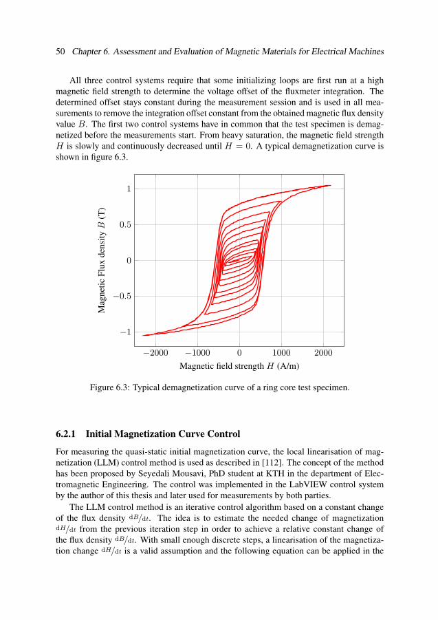
50 Chapter 6. Assessment and Evaluation of Magnetic Materials for Electrical Machines
All three control systems require that some initializing loops are first run at a highmagnetic field strength to determine the voltage offset of the fluxmeter integration. Thedetermined offset stays constant during the measurement session and is used in all mea-surements to remove the integration offset constant from the obtained magnetic flux densityvalue B. The first two control systems have in common that the test specimen is demag-netized before the measurements start. From heavy saturation, the magnetic field strengthH is slowly and continuously decreased until H = 0. A typical demagnetization curve isshown in figure 6.3.
−2000 −1000 0 1000 2000
−1
−0.5
0
0.5
1
Magnetic field strength H (A/m)
Mag
neti
cF
lux
dens
ity
B(T
)
Figure 6.3: Typical demagnetization curve of a ring core test specimen.
6.2.1 Initial Magnetization Curve Control
For measuring the quasi-static initial magnetization curve, the local linearisation of mag-netization (LLM) control method is used as described in [112]. The concept of the methodhas been proposed by Seyedali Mousavi, PhD student at KTH in the department of Elec-tromagnetic Engineering. The control was implemented in the LabVIEW control systemby the author of this thesis and later used for measurements by both parties.
The LLM control method is an iterative control algorithm based on a constant changeof the flux density dB/dt. The idea is to estimate the needed change of magnetizationdH/dt from the previous iteration step in order to achieve a relative constant change ofthe flux density dB/dt. With small enough discrete steps, a linearisation of the magnetiza-tion change dH/dt is a valid assumption and the following equation can be applied in the

6.2. Measurement Setup 51
algorithm
(dH/dt)n+1 = (dB/dt)ref ·
(
dH
dB
)
n
. (6.1)
In (6.1),(
dHdB
)
nis the slope of the initial magnetization curve from the previous iteration
step n. The LLM control method is started after a continuous demagnetization process,e.g. the magnetic working point of the material lies in the origin (B and H are zero). Forthe first few steps, the so-called transition time, a small constant value of dH/dB (between0.2 and 1) is used to initialize the process. Best results were reached with transition timesbetween 10 ms and 30 ms (based on practical evaluation). After the transition time, theiterative LLM control method starts from the last transition step and H increases contin-uously until a maximum predefined magnetic field strength value. This value is based ona maximum current of around 6 A and thus depending on the test specimen and its pri-mary excitation winding. Typical reached magnetic field strength values were between3000 A/m and 6000 A/m.
To avoid dynamic effects in the initial magnetization curve, a constant dB/dt is chosenwhich yields a magnetization time of 10 s to 20 s from zero flux density until full satu-rated magnetization, as it is shown in figure 6.4. This equals for the full hysteresis loop amaximum equivalent magnetization frequency of feq = 1
4·10 s = 25 mHz and makes eddycurrent effects negligible.
0 500 1000 1500 2000 2500 30000
0.5
1
1.5
Magnetic field strength H (A/m)
Mag
neti
cfl
uxde
nsit
yB
(T)
Figure 6.4: Initial magnetization curve with a constant dB/dt of 0.02 T/s
6.2.2 AC Measurements Control System
Characterizing magnetic materials by their BH hysteresis loop and iron losses requiresvariable magnetic flux density peak values B and frequencies f . An iterative algorithm
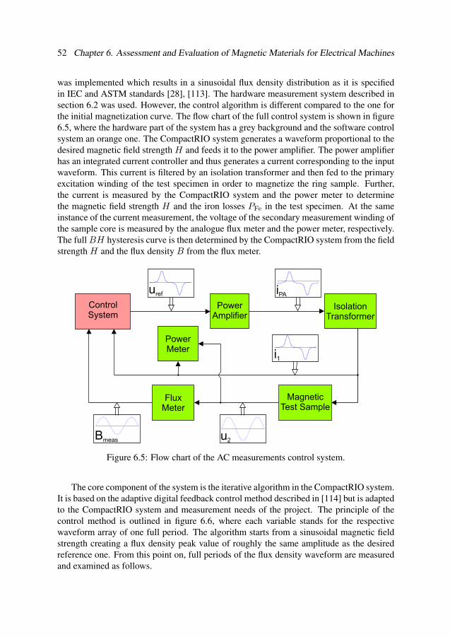
52 Chapter 6. Assessment and Evaluation of Magnetic Materials for Electrical Machines
was implemented which results in a sinusoidal flux density distribution as it is specifiedin IEC and ASTM standards [28], [113]. The hardware measurement system described insection 6.2 was used. However, the control algorithm is different compared to the one forthe initial magnetization curve. The flow chart of the full control system is shown in figure6.5, where the hardware part of the system has a grey background and the software controlsystem an orange one. The CompactRIO system generates a waveform proportional to thedesired magnetic field strength H and feeds it to the power amplifier. The power amplifierhas an integrated current controller and thus generates a current corresponding to the inputwaveform. This current is filtered by an isolation transformer and then fed to the primaryexcitation winding of the test specimen in order to magnetize the ring sample. Further,the current is measured by the CompactRIO system and the power meter to determinethe magnetic field strength H and the iron losses PFe in the test specimen. At the sameinstance of the current measurement, the voltage of the secondary measurement winding ofthe sample core is measured by the analogue flux meter and the power meter, respectively.The full BH hysteresis curve is then determined by the CompactRIO system from the fieldstrength H and the flux density B from the flux meter.
PowerAmplifier
ControlSystem
IsolationTransformer
MagneticTest Sample
FluxMeter
uref iPA
u2Bmeas
i1
PowerMeter
Figure 6.5: Flow chart of the AC measurements control system.
The core component of the system is the iterative algorithm in the CompactRIO system.It is based on the adaptive digital feedback control method described in [114] but is adaptedto the CompactRIO system and measurement needs of the project. The principle of thecontrol method is outlined in figure 6.6, where each variable stands for the respectivewaveform array of one full period. The algorithm starts from a sinusoidal magnetic fieldstrength creating a flux density peak value of roughly the same amplitude as the desiredreference one. From this point on, full periods of the flux density waveform are measuredand examined as follows.

6.2. Measurement Setup 53
First, the measured flux density Bmeas (one full period) is filtered by a harmonic filterto eliminate any undesirable DC and high frequency content. This is achieved by trans-ferring the signal to the frequency domain with a fast-Fourier transformation. From thefrequency domain signal, only the lowest 9 to 23 harmonics are then transformed backto the time domain by an inverse fast-Fourier transformation. Comparing the filtered fluxdensity waveform BFFT with the sinusoidal reference one Bref yields then ∆B, the dif-ference between each element of the waveform (one period). ∆B is then multiplied withthe constant gain (proportional controller) before it is added to the output waveform Un−1
ref
of the previous iteration step to become Unref . This signal waveform is the new reference
voltage output for the current controller of the power amplifier.However, not only the waveform of the reference signal has to be adapted. There is also
a varying phase difference between the measured flux density and the generated currentfor the corresponding magnetic field strength. It is depending on the integrated currentcontroller of the power amplifier, the isolation transformer and the magnetic test sample.To correct this phase error, the fundamental phase of Un+1
gain is determined and compared tothe fundamental phase of the current in the excitation winding to determine ∆ϕ. Again,a proportional controller is used and the resulting phase correction is added to the phasedifference of the previous iteration ϕn−1
ref . The new phase angle ϕn+1ref is used to shift the
reference voltage Un+1ref in order to feed the corrected waveform to the current controller
of the power amplifier.
PhaseShift
GainHarmonic
Filter
Gain
ExternalSystem
in(1)
Bmeas
urefAmp
un(1)
Bref
nref
)BBmeasFFT uref
)n
imeas
Figure 6.6: Flow chart of the iterative control system algorithm.
The gain for the waveform correction and the phase correction has to be chosen care-fully. If it is too large, oscillation occurs and the system can become unstable. Too smallvalues will reduce the system settling time and could be filtered as noise. Thus, a tradeoff has to be made between the stability of the system and the number of needed iterationsin order to achieve a sinusoidal flux density. For the waveform correction gain, valuesin the range of 1 × 10⁻³ to 1 × 10⁻² have shown to keep the system stable at reasonablesettling times (5 s to 20 s for 50 Hz measurements). Further improvements of the controlsystem and parameters were down-prioritized due to time constraints in the project. The
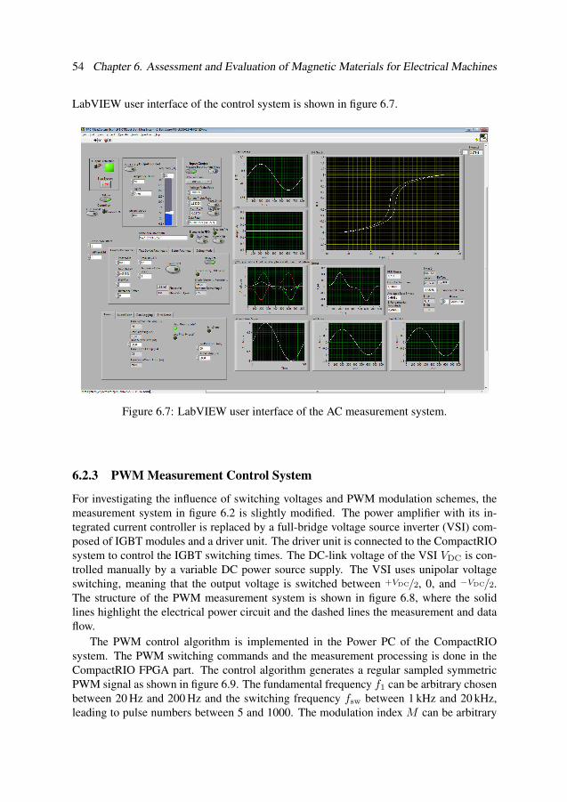
54 Chapter 6. Assessment and Evaluation of Magnetic Materials for Electrical Machines
LabVIEW user interface of the control system is shown in figure 6.7.
Figure 6.7: LabVIEW user interface of the AC measurement system.
6.2.3 PWM Measurement Control System
For investigating the influence of switching voltages and PWM modulation schemes, themeasurement system in figure 6.2 is slightly modified. The power amplifier with its in-tegrated current controller is replaced by a full-bridge voltage source inverter (VSI) com-posed of IGBT modules and a driver unit. The driver unit is connected to the CompactRIOsystem to control the IGBT switching times. The DC-link voltage of the VSI VDC is con-trolled manually by a variable DC power source supply. The VSI uses unipolar voltageswitching, meaning that the output voltage is switched between +VDC/2, 0, and −VDC/2.The structure of the PWM measurement system is shown in figure 6.8, where the solidlines highlight the electrical power circuit and the dashed lines the measurement and dataflow.
The PWM control algorithm is implemented in the Power PC of the CompactRIOsystem. The PWM switching commands and the measurement processing is done in theCompactRIO FPGA part. The control algorithm generates a regular sampled symmetricPWM signal as shown in figure 6.9. The fundamental frequency f1 can be arbitrary chosenbetween 20 Hz and 200 Hz and the switching frequency fsw between 1 kHz and 20 kHz,leading to pulse numbers between 5 and 1000. The modulation index M can be arbitrary

6.2. Measurement Setup 55
FPGA
A/D-DOAVSI
PM
Powermeter
Inverter
RT
System
FM
Fluxmeter
Control System Stator Core
Figure 6.8: Overview on the measurement setup for PWM excitation. Solid lines indicatethe electric power circuit and dashed lines the measurement and data flow.
varied in the linear modulation region between 0.2 and 0.9. It is defined as [115]
M =U1
UDC/2, (6.2)
with U1 being the amplitude of the desired fundamental sinus waveform and UDC the DC-link voltage of the inverter. Over-modulation is not investigated in this work. The uppermodulation limit of 0.9 is chosen due to the dead-time limitations of the VSI driver unitand the IGBT modules.
Time
Vol
tage
Figure 6.9: Regular sampled symmetric signal of the PWM measurement system with amodulation index of 0.7.
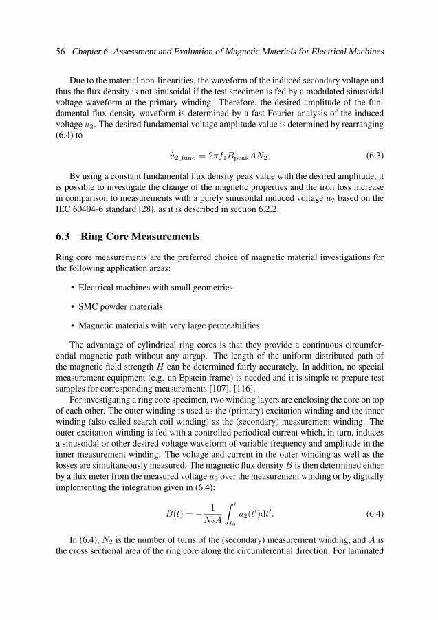
56 Chapter 6. Assessment and Evaluation of Magnetic Materials for Electrical Machines
Due to the material non-linearities, the waveform of the induced secondary voltage andthus the flux density is not sinusoidal if the test specimen is fed by a modulated sinusoidalvoltage waveform at the primary winding. Therefore, the desired amplitude of the fun-damental flux density waveform is determined by a fast-Fourier analysis of the inducedvoltage u2. The desired fundamental voltage amplitude value is determined by rearranging(6.4) to
u2_fund = 2πf1BpeakAN2, (6.3)
By using a constant fundamental flux density peak value with the desired amplitude, itis possible to investigate the change of the magnetic properties and the iron loss increasein comparison to measurements with a purely sinusoidal induced voltage u2 based on theIEC 60404-6 standard [28], as it is described in section 6.2.2.
6.3 Ring Core Measurements
Ring core measurements are the preferred choice of magnetic material investigations forthe following application areas:
• Electrical machines with small geometries
• SMC powder materials
• Magnetic materials with very large permeabilities
The advantage of cylindrical ring cores is that they provide a continuous circumfer-ential magnetic path without any airgap. The length of the uniform distributed path ofthe magnetic field strength H can be determined fairly accurately. In addition, no specialmeasurement equipment (e.g. an Epstein frame) is needed and it is simple to prepare testsamples for corresponding measurements [107], [116].
For investigating a ring core specimen, two winding layers are enclosing the core on topof each other. The outer winding is used as the (primary) excitation winding and the innerwinding (also called search coil winding) as the (secondary) measurement winding. Theouter excitation winding is fed with a controlled periodical current which, in turn, inducesa sinusoidal or other desired voltage waveform of variable frequency and amplitude in theinner measurement winding. The voltage and current in the outer winding as well as thelosses are simultaneously measured. The magnetic flux density B is then determined eitherby a flux meter from the measured voltage u2 over the measurement winding or by digitallyimplementing the integration given in (6.4):
B(t) = −1
N2A
∫ t
t0
u2(t′)dt′. (6.4)
In (6.4), N2 is the number of turns of the (secondary) measurement winding, and A isthe cross sectional area of the ring core along the circumferential direction. For laminated

6.4. Conclusions 57
cores, this area is determined by
A =2m
γ(Do + Di)π, (6.5)
where m is the total mass of the core specimen and γ the mass density of the laminationmaterial. Do and Di are the outer and inner diameter of the cylinder, respectively. Forpowder materials, A is solely determined by the core diameters and its length lm:
A =(Do − Di)lm
2(6.6)
The magnetic field strength H is determined from the measured excitation windingcurrent i1 using (6.7). In (6.7), lm is the mean length of the magnetic path in the ring coresample and N1 is the number of turns of the primary (excitation) winding:
H(t) =N1i1(t)
lm. (6.7)
For closed ring cores, lm is determined depending on the ratio between the outer (Do)and inner diameter (Di) of the cylinder as suggested in [107]. If the ratio fulfils Do/Di ≤1.1, as recommended in the standard [28], the mean length should be determined by lm =π(Do + Di)/2. For larger ratios of Do/Di, the mean length of the magnetic path in thecross section should be determined by (6.8) to correct for the non-uniformity field over thecross section area:
lm =π(Do − Di)
ln(Do/Di). (6.8)
The derivation of (6.8) is presented in [107].Finally, the voltage of the inner winding and the current in the outer winding are simul-
taneously measured to determine the instantaneous iron losses in the core by
P (t) =N1
N2i1(t)u2(t). (6.9)
6.4 Conclusions
Magnetic materials for electrical machines can be investigated by different methods. Thedetermination of the magnetic material characteristics and the iron losses is usually car-ried out on the Epstein frame. But also ring core tests and single-sheet measurements areapplied for the material characterisation. A measurement system for investigating mag-netic materials and iron losses in electrical machine parts has been developed and setupin the departments’ laboratory. The test bench can be used with an Epstein frame or withring core test specimen. The possible material characteristics which can be determinedby the system are the initial BH magnetization curve, and the full BH hysteresis loopsand iron losses for purely sinusoidal flux densities of arbitrary amplitudes. Furthermore,
58 Chapter 6. Assessment and Evaluation of Magnetic Materials for Electrical Machines
the full BH hysteresis loops and the iron losses can be measured for pulse-width modu-lation switching schemes of different frequency and amplitude (variable DC-link voltage).All slot-less stator core measurements in the following chapters are performed with thismeasurement system.
Chapter 7
Welding Influence on the Performance
of PMSM with NiFe and SiFe Stator
Laminations
The lamination sheets of electrical machine stator cores are usually welded to withstand
the mechanical stresses during the machine operation. The welding seams deteriorate the
magnetic material locally and lead to increased iron losses, especially at high operating
speeds. The influence of the welding process is studied using small stator cores of a slot-
less PMSM from an industrial hand tool with a maximum speed of up to 36 000 rpm. A total
of eight cores of the same dimensions but with different materials, different lamination
thicknesses, as well as with and without welding seams are experimentally investigated.
The analysis and comparison of the measurement values lead to a quantification of the
influence of welding on the core iron losses and motor performance.
7.1 Investigated Stator Cores
Two winding layers are enclosing the yoke of each investigated stator core. The coresare made from thin SiFe (0.2 mm lamination thickness) and NiFe (0.1 mm and 0.2 mmlamination thickness) steel sheets. The SiFe cores have a silicon content of approximately3% and an inorganic phosphate based coating. The NiFe sheets are made of approximately40% nickel and have an inorganic zircon based coating. Table 7.1 gives an overview of theother material properties. These values were provided by the sheet manufacturers.
The NiFe sheets have gone through a stress-relief annealing process after they werelaser cut and before they were glued and welded together. The annealing process restoresthe magnetic properties due to the deterioration of the cutting process [117], [118]. TheSiFe lamination sheets, provided by another manufacturer, did not receive a thermal treat-ment during the manufacturing process.
Each core is 64.5 mm long and has an outer and inner diameter of 31 mm and 23.2 mm,respectively. Since the ratio of the outer to the inner diameter is Do/Di = 1.34, the
59
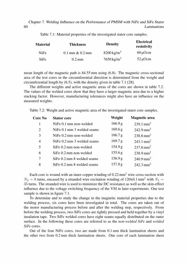
60Chapter 7. Welding Influence on the Performance of PMSM with NiFe and SiFe Stator
Laminations
Table 7.1: Material properties of the investigated stator core samples.
Material Thickness DensityElectrical
resistivity
NiFe 0.1 mm & 0.2 mm 8200 kg/m3 60 µΩcm
SiFe 0.2 mm 7650 kg/m3 52 µΩcm
mean length of the magnetic path is 84.55 mm using (6.8). The magnetic cross-sectionalarea of the test cores in the circumferential direction is determined from the weight andcircumferential length by (6.5), with the density given in table 7.1 [28].
The different weights and active magnetic areas of the cores are shown in table 7.2.The values of the welded cores show that they have a larger magnetic area due to a higherstacking factor. However, manufacturing tolerances might also have an influence on themeasured weights.
Table 7.2: Weight and active magnetic area of the investigated stator core samples.
Core No Stator core Weight Magnetic area
1 NiFe 0.1 mm non-welded 166.9 g 239.1 mm2
2 NiFe 0.1 mm 3 welded seams 169.6 g 242.9 mm2
3 NiFe 0.2 mm non-welded 166.7 g 238.8 mm2
4 NiFe 0.2 mm 3 welded seams 169.7 g 243.1 mm2
5 SiFe 0.2 mm non-welded 154.9 g 237.8 mm2
6 SiFe 0.2 mm non-welded 155.6 g 238.9 mm2
7 SiFe 0.2 mm 8 welded seams 156.9 g 240.9 mm2
8 SiFe 0.2 mm 8 welded seams 157.8 g 242.3 mm2
Each core is wound with an inner copper winding of 0.22 mm2 wire cross-section withN2 = 8 turns, encased by a stranded wire excitation winding of 120x0.1 mm2 with N1 =35 turns. The stranded wire is used to minimize the DC resistance as well as the skin-effectinfluence due to the voltage switching frequency of the VSI in later experiments. One testsample is shown in figure 7.1.
To determine and to study the change in the magnetic material properties due to thewelding process, six cores have been investigated in total. The cores are taken out ofthe motor manufacturing process before and after the welding step, respectively. Frombefore the welding process, two SiFe cores are tightly pressed and held together by a vinylinsulation tape. Two SiFe welded cores have eight seams equally distributed on the outersurface. In the following these cores are referred to as the non-welded SiFe and welded
SiFe cores.Out of the four NiFe cores, two are made from 0.1 mm thick lamination sheets and
the other two from 0.2 mm thick lamination sheets. One core of each lamination sheet

7.2. Measurement Results 61
Figure 7.1: Investigated stator core with stranded wire excitation winding.
thickness is non-welded and the sheets are glued together. These are referred to as non-
welded NiFe cores. The other two are welded by three welding seams equally distributedon the outer surface and referred to as welded NiFe cores.
Pictures of a welded SiFe and a welded NiFe core are shown in figure 7.2. Whenlooking closely at the front side of the NiFe core, the welding seams have not visiblydamaged the core locally. A magnification of the welding seams of the SiFe and NiFe statorcores is shown in figure 7.3. It should be noted that the magnification level is different inthe two figures.
7.2 Measurement Results
In the following, the measured average values are given for the two welded and two non-welded SiFe stator cores, respectively, since it is not possible to visualize the individualcurves in the plots. The maximum derivation between two results is less than 3%. In orderto increase the readability and avoid clutter, only a selection of all measured points areshown in figure 7.4 and figure 7.5.
The initial BH magnetization curves of all investigated materials are shown in fig-ure 7.4 up to a maximum magnetic field of H = 3000 A/m. The curves are measured witha controlled flux density change dB/dt as described in section 6.2.1. Between 0.2 T and1.2 T, the incremental permeability ( ∆B
∆H) is lower for the welded stator cores, compared
to their non-welded counterparts. The figure indicates that the welding process influencesmainly the linear, non-saturated region of the cores. Figure 7.4 shows further the strongsaturation behaviour of NiFe. For high magnetic field strengths (H > 2500 A/m) the in-cremental permeability of NiFe becomes even smaller compared to the SiFe incrementalpermeability. This means SiFe can reach higher flux density values compared to NiFe butonly at high magnetic fields (H > 2700 A/m in this case).
The welding process also leads to a decrease of the relative amplitude permeability µr
of the lamination sheets, as it is shown in figure 7.5. The relative amplitude permeability
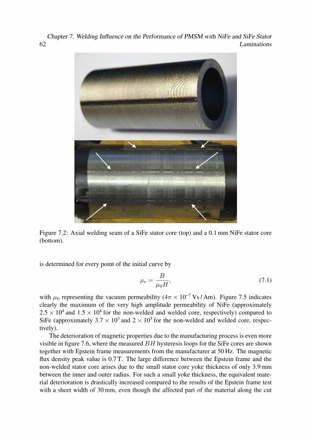
62Chapter 7. Welding Influence on the Performance of PMSM with NiFe and SiFe Stator
Laminations
Figure 7.2: Axial welding seam of a SiFe stator core (top) and a 0.1 mm NiFe stator core(bottom).
is determined for every point of the initial curve by
µr =B
µ0H, (7.1)
with µ0 representing the vacuum permeability (4π × 10−7 Vs / Am). Figure 7.5 indicatesclearly the maximum of the very high amplitude permeability of NiFe (approximately2.5 × 104 and 1.5 × 10⁴ for the non-welded and welded core, respectively) compared toSiFe (approximately 3.7 × 10³ and 2 × 10³ for the non-welded and welded core, respec-tively).
The deterioration of magnetic properties due to the manufacturing process is even morevisible in figure 7.6, where the measured BH hysteresis loops for the SiFe cores are showntogether with Epstein frame measurements from the manufacturer at 50 Hz. The magneticflux density peak value is 0.7 T. The large difference between the Epstein frame and thenon-welded stator core arises due to the small stator core yoke thickness of only 3.9 mmbetween the inner and outer radius. For such a small yoke thickness, the equivalent mate-rial deterioration is drastically increased compared to the results of the Epstein frame testwith a sheet width of 30 mm, even though the affected part of the material along the cut
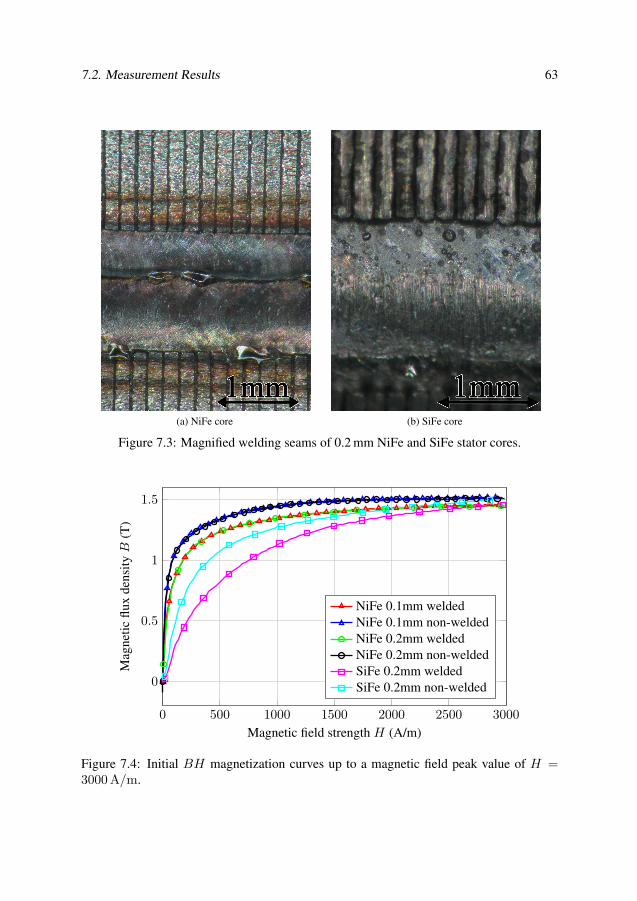
7.2. Measurement Results 63
(a) NiFe core (b) SiFe core
Figure 7.3: Magnified welding seams of 0.2 mm NiFe and SiFe stator cores.
0 500 1000 1500 2000 2500 3000
0
0.5
1
1.5
Magnetic field strength H (A/m)
Mag
neti
cfl
uxde
nsit
yB
(T)
NiFe 0.1mm weldedNiFe 0.1mm non-weldedNiFe 0.2mm weldedNiFe 0.2mm non-weldedSiFe 0.2mm weldedSiFe 0.2mm non-welded
Figure 7.4: Initial BH magnetization curves up to a magnetic field peak value of H =3000 A/m.

64Chapter 7. Welding Influence on the Performance of PMSM with NiFe and SiFe Stator
Laminations
0 50 100 150 200 250 300 350 4000
1
2
3
Magnetic field strength H (A/m)
Mag
neti
cpe
rmea
bili
tyµ
r(x
104)
NiFe 0.1mm weldedNiFe 0.1mm non-weldedNiFe 0.2mm weldedNiFe 0.2mm non-weldedSiFe 0.2mm weldedSiFe 0.2mm non-welded
Figure 7.5: Amplitude permeability µr of the non-welded and welded stator cores.
edges would be similar. There is almost no saturation in the Epstein frame measurements atsuch low flux density values of 0.7 T. Therefore, the increase of the coercive field strengthHc by 53 % between the dashed black (Epstein frame) and the cyan (non-welded) hystere-sis curve in figure 7.6 indicates clearly the influence of the stress induced by the cuttingprocess. Similar results between Epstein frame tests and smaller ring core measurementswere obtained in [119]. The large difference between the cyan (non-welded) and magenta(welded) hysteresis curve (55 % increase) is most likely due to the deterioration of thematerial properties and stress in the area of the eight welding seams.
The deterioration of magnetic properties due to the welding process is investigated bythe full BH hysteresis loop of the NiFe stator cores in figure 7.7 for the welded and thenon-welded stator cores at 50 Hz and a maximum magnetic flux density of 1.2 T. One canclearly see the smaller slope (relative amplitude permeability) and larger magnetic fieldstrength for a certain magnetic flux density in the saturation region.
A study of the magnetic coercivity in figure 7.8 (this figure is a zoom of figure 7.7)shows that the 0.2 mm welded cores have a 37 % higher magnetic coercive field comparedto the non-welded cores. For the 0.1 mm cores the magnetic coercive field increase is23 %. This increase is most likely due to the welding seams that partly destroy the sheetinsulation layer. However, the applied axial forces during the welding process also damagethe insulation layer and introduce stress in the lamination sheets. This increases the amountof eddy current losses as well [59].
The larger increase in the area of the hysteresis curves for the welded cores is alsoreflected in the iron loss measurements. The iron losses are determined by the absolute
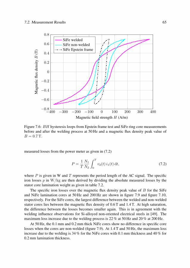
7.2. Measurement Results 65
−400 −300 −200 −100 0 100 200 300 400−0.8
−0.6
−0.4
−0.2
0
0.2
0.4
0.6
0.8
Magnetic field strength H (A/m)
Mag
neti
cfl
uxde
nsit
yB
(T)
SiFe weldedSiFe non-weldedSiFe Epstein frame
Figure 7.6: BH hysteresis loops from Epstein frame test and SiFe ring core measurementsbefore and after the welding process at 50 Hz and a magnetic flux density peak value ofB = 0.7 T.
measured losses from the power meter as given in (7.2)
P =1
T
N1
N2
∫ T
0
v2(t) i1(t) dt, (7.2)
where P is given in W and T represents the period length of the AC signal. The specificiron losses p in W/kg are then derived by dividing the absolute measured losses by thestator core lamination weight as given in table 7.2.
The specific iron losses over the magnetic flux density peak value of B for the SiFeand NiFe lamination cores at 50 Hz and 200 Hz are shown in figure 7.9 and figure 7.10,respectively. For the SiFe cores, the largest difference between the welded and non-weldedstator cores lies between the magnetic flux density of 0.6 T and 1.4 T. At high saturation,the difference between the losses becomes smaller again. This is in agreement with thewelding influence observations for Si-alloyed non-oriented electrical steels in [49]. Themaximum loss increase due to the welding process is 22 % at 50 Hz and 20 % at 200 Hz.
At 50 Hz, the 0.1 mm and 0.2 mm thick NiFe cores show no difference in specific corelosses when the cores are non-welded (figure 7.9). At 1.4 T and 50 Hz, the maximum lossincrease due to the welding is 34 % for the NiFe cores with 0.1 mm thickness and 40 % for0.2 mm lamination thickness.

66Chapter 7. Welding Influence on the Performance of PMSM with NiFe and SiFe Stator
Laminations
−500 −400 −300 −200 −100 0 100 200 300 400 500−1.5
−1
−0.5
0
0.5
1
1.5
Zoom
Magnetic field strength H (A/m)
Mag
neti
cfl
uxde
nsit
yB
(T)
0.1mm welded0.1mm non-welded0.2mm welded0.2mm non-welded
Figure 7.7: Welded and non-welded NiFe BH hysteresis loops at 50 Hz and a magneticflux density peak value of B = 1.2 T.
However, the loss distribution between the NiFe cores is different at 200 Hz as shownin figure 7.10. At this frequency, it can be observed that the difference between the twonon-welded cores is significant. The losses are heavily depending on the sheet thickness.The 0.2 mm non-welded core has slightly lower losses compared to the 0.1 mm welded oneat low flux density values, but for flux density values B > 0.9 T, the 0.2 mm non-weldedcore has a larger loss increase.
The specific iron losses of all investigated stator cores for frequencies between 10 Hzand 200 Hz and a magnetic flux density peak value of B = 1.4 T are shown in figure 7.11.
The welding effect of the stator cores can be observed by the increasing differencein the specific core losses due to the eddy currents between the sheets. At 200 Hz, thisyields to a loss increase between the non-welded and the welded cores of 22.9 % for theSiFe cores, 29.1 % for the 0.1 mm NiFe cores, and 33.2 % for the 0.2 mm NiFe cores,respectively.
Figure 7.12 presents the specific core loss per cycle (E = p/f with E in Ws) over thefrequency for the NiFe cores, to allow a separation of the total losses into hysteresis losses(physt) and eddy current losses (pec). Using the iron loss separation approach (7.3), thehysteresis losses are constant and the eddy current losses are proportional to the frequency
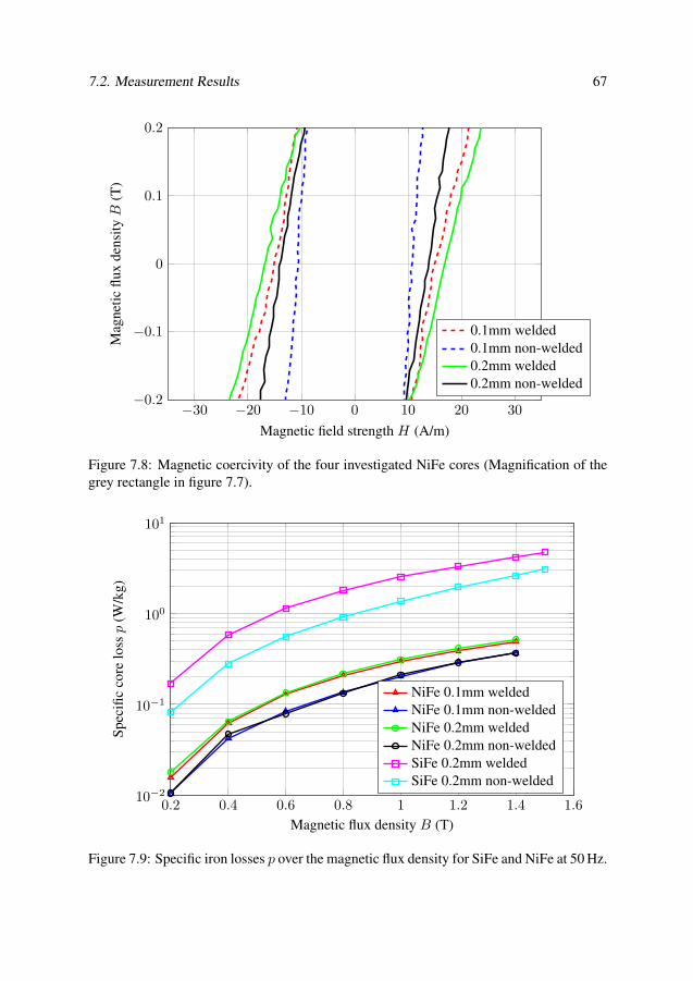
7.2. Measurement Results 67
−30 −20 −10 0 10 20 30−0.2
−0.1
0
0.1
0.2
Magnetic field strength H (A/m)
Mag
neti
cfl
uxde
nsit
yB
(T)
0.1mm welded0.1mm non-welded0.2mm welded0.2mm non-welded
Figure 7.8: Magnetic coercivity of the four investigated NiFe cores (Magnification of thegrey rectangle in figure 7.7).
0.2 0.4 0.6 0.8 1 1.2 1.4 1.610−2
10−1
100
101
Magnetic flux density B (T)
Spe
cifi
cco
relo
ssp
(W/k
g)
NiFe 0.1mm weldedNiFe 0.1mm non-weldedNiFe 0.2mm weldedNiFe 0.2mm non-weldedSiFe 0.2mm weldedSiFe 0.2mm non-welded
Figure 7.9: Specific iron losses p over the magnetic flux density for SiFe and NiFe at 50 Hz.
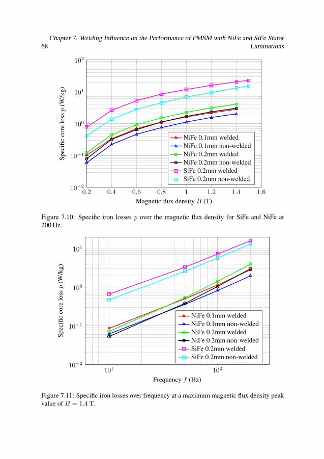
68Chapter 7. Welding Influence on the Performance of PMSM with NiFe and SiFe Stator
Laminations
0.2 0.4 0.6 0.8 1 1.2 1.4 1.610−2
10−1
100
101
102
Magnetic flux density B (T)
Spe
cifi
cco
relo
ssp
(W/k
g)
NiFe 0.1mm weldedNiFe 0.1mm non-weldedNiFe 0.2mm weldedNiFe 0.2mm non-weldedSiFe 0.2mm weldedSiFe 0.2mm non-welded
Figure 7.10: Specific iron losses p over the magnetic flux density for SiFe and NiFe at200 Hz.
101 10210−2
10−1
100
101
Frequency f (Hz)
Spe
cifi
cco
relo
ssp
(W/k
g)
NiFe 0.1mm weldedNiFe 0.1mm non-weldedNiFe 0.2mm weldedNiFe 0.2mm non-weldedSiFe 0.2mm weldedSiFe 0.2mm non-welded
Figure 7.11: Specific iron losses over frequency at a maximum magnetic flux density peakvalue of B = 1.4 T.
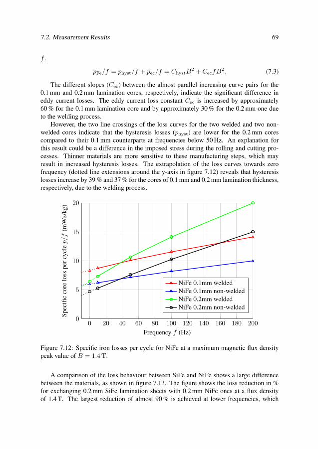
7.2. Measurement Results 69
f .
pFe/f = physt/f + pec/f = ChystB2 + CecfB2. (7.3)
The different slopes (Cec) between the almost parallel increasing curve pairs for the0.1 mm and 0.2 mm lamination cores, respectively, indicate the significant difference ineddy current losses. The eddy current loss constant Cec is increased by approximately60 % for the 0.1 mm lamination core and by approximately 30 % for the 0.2 mm one dueto the welding process.
However, the two line crossings of the loss curves for the two welded and two non-welded cores indicate that the hysteresis losses (physt) are lower for the 0.2 mm corescompared to their 0.1 mm counterparts at frequencies below 50 Hz. An explanation forthis result could be a difference in the imposed stress during the rolling and cutting pro-cesses. Thinner materials are more sensitive to these manufacturing steps, which mayresult in increased hysteresis losses. The extrapolation of the loss curves towards zerofrequency (dotted line extensions around the y-axis in figure 7.12) reveals that hysteresislosses increase by 39 % and 37 % for the cores of 0.1 mm and 0.2 mm lamination thickness,respectively, due to the welding process.
0 20 40 60 80 100 120 140 160 180 2000
5
10
15
20
Frequency f (Hz)
Spe
cifi
cco
relo
sspe
rcy
cle
p/f
(mW
s/kg
)
NiFe 0.1mm weldedNiFe 0.1mm non-weldedNiFe 0.2mm weldedNiFe 0.2mm non-welded
Figure 7.12: Specific iron losses per cycle for NiFe at a maximum magnetic flux densitypeak value of B = 1.4 T.
A comparison of the loss behaviour between SiFe and NiFe shows a large differencebetween the materials, as shown in figure 7.13. The figure shows the loss reduction in %for exchanging 0.2 mm SiFe lamination sheets with 0.2 mm NiFe ones at a flux densityof 1.4 T. The largest reduction of almost 90 % is achieved at lower frequencies, which
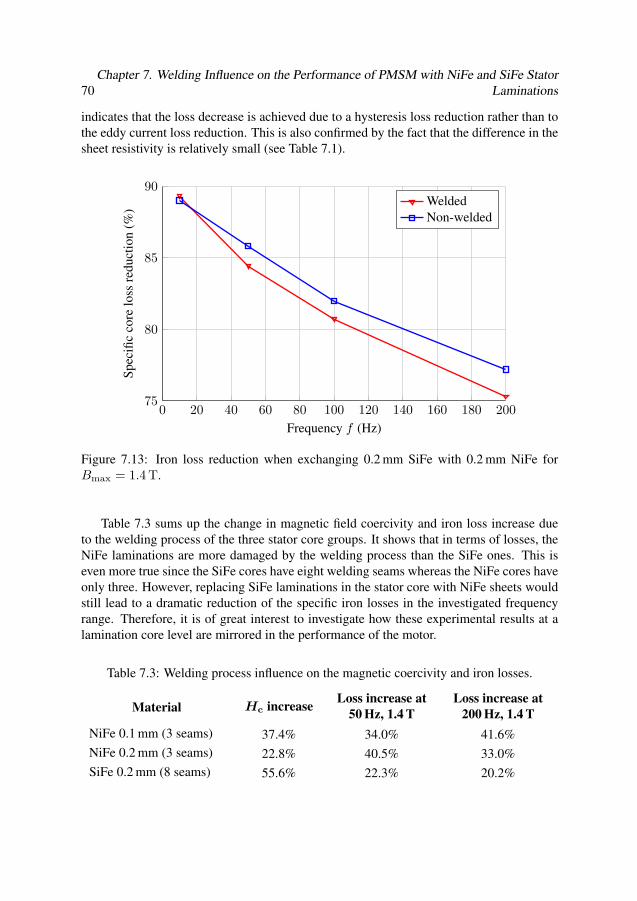
70Chapter 7. Welding Influence on the Performance of PMSM with NiFe and SiFe Stator
Laminations
indicates that the loss decrease is achieved due to a hysteresis loss reduction rather than tothe eddy current loss reduction. This is also confirmed by the fact that the difference in thesheet resistivity is relatively small (see Table 7.1).
0 20 40 60 80 100 120 140 160 180 20075
80
85
90
Frequency f (Hz)
Spe
cifi
cco
relo
ssre
duct
ion
(%)
WeldedNon-welded
Figure 7.13: Iron loss reduction when exchanging 0.2 mm SiFe with 0.2 mm NiFe forBmax = 1.4 T.
Table 7.3 sums up the change in magnetic field coercivity and iron loss increase dueto the welding process of the three stator core groups. It shows that in terms of losses, theNiFe laminations are more damaged by the welding process than the SiFe ones. This iseven more true since the SiFe cores have eight welding seams whereas the NiFe cores haveonly three. However, replacing SiFe laminations in the stator core with NiFe sheets wouldstill lead to a dramatic reduction of the specific iron losses in the investigated frequencyrange. Therefore, it is of great interest to investigate how these experimental results at alamination core level are mirrored in the performance of the motor.
Table 7.3: Welding process influence on the magnetic coercivity and iron losses.
Material Hc increaseLoss increase at
50 Hz, 1.4 T
Loss increase at
200 Hz, 1.4 T
NiFe 0.1 mm (3 seams) 37.4% 34.0% 41.6%
NiFe 0.2 mm (3 seams) 22.8% 40.5% 33.0%
SiFe 0.2 mm (8 seams) 55.6% 22.3% 20.2%
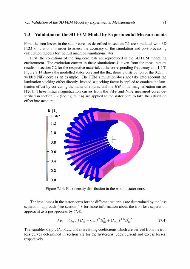
7.3. Validation of the 3D FEM Model by Experimental Measurements 71
7.3 Validation of the 3D FEM Model by Experimental Measurements
First, the iron losses in the stator cores as described in section 7.1 are simulated with 3DFEM simulations in order to assess the accuracy of the simulation and post-processingcalculation models for the full machine simulations later.
First, the conditions of the ring core tests are reproduced in the 3D FEM modellingenvironment. The excitation current in these simulations is taken from the measurementresults in section 7.2 for the respective material, at the corresponding frequency and 1.4 T.Figure 7.14 shows the modelled stator core and the flux density distribution of the 0.2 mmwelded NiFe core as an example. The FEM simulation does not take into account thelamination stacking effect directly. Instead, a stacking factor is applied to emulate the lam-ination effect by correcting the material volume and the BH initial magnetization curves[120]. These initial magnetization curves from the SiFe and NiFe measured cores de-scribed in section 7.2 (see figure 7.4) are applied to the stator core to take the saturationeffect into account.
Figure 7.14: Flux density distribution in the wound stator core.
The iron losses in the stator cores for the different materials are determined by the lossseparation approach (see section 4.3 for more information about the iron loss separationapproach) as a post-process by (7.4).
PFe = ChystfBαm + Cecf2B2
m + Cexcf1.5B1.5m . (7.4)
The variables Chyst, Cec, Cexc and α are fitting coefficients which are derived from the ironloss curves determined in section 7.2 for the hysteresis, eddy current and excess losses,respectively.
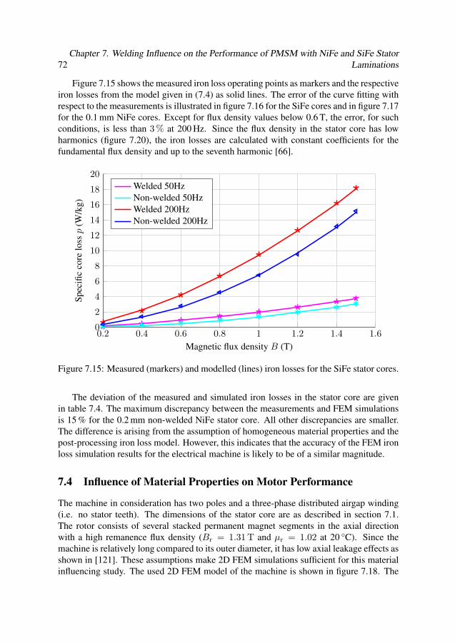
72Chapter 7. Welding Influence on the Performance of PMSM with NiFe and SiFe Stator
Laminations
Figure 7.15 shows the measured iron loss operating points as markers and the respectiveiron losses from the model given in (7.4) as solid lines. The error of the curve fitting withrespect to the measurements is illustrated in figure 7.16 for the SiFe cores and in figure 7.17for the 0.1 mm NiFe cores. Except for flux density values below 0.6 T, the error, for suchconditions, is less than 3 % at 200 Hz. Since the flux density in the stator core has lowharmonics (figure 7.20), the iron losses are calculated with constant coefficients for thefundamental flux density and up to the seventh harmonic [66].
0.2 0.4 0.6 0.8 1 1.2 1.4 1.60
2
4
6
8
10
12
14
16
18
20
Magnetic flux density B (T)
Spe
cifi
cco
relo
ssp
(W/k
g)
Welded 50HzNon-welded 50HzWelded 200HzNon-welded 200Hz
Figure 7.15: Measured (markers) and modelled (lines) iron losses for the SiFe stator cores.
The deviation of the measured and simulated iron losses in the stator core are givenin table 7.4. The maximum discrepancy between the measurements and FEM simulationsis 15 % for the 0.2 mm non-welded NiFe stator core. All other discrepancies are smaller.The difference is arising from the assumption of homogeneous material properties and thepost-processing iron loss model. However, this indicates that the accuracy of the FEM ironloss simulation results for the electrical machine is likely to be of a similar magnitude.
7.4 Influence of Material Properties on Motor Performance
The machine in consideration has two poles and a three-phase distributed airgap winding(i.e. no stator teeth). The dimensions of the stator core are as described in section 7.1.The rotor consists of several stacked permanent magnet segments in the axial directionwith a high remanence flux density (Br = 1.31 T and µr = 1.02 at 20 C). Since themachine is relatively long compared to its outer diameter, it has low axial leakage effects asshown in [121]. These assumptions make 2D FEM simulations sufficient for this materialinfluencing study. The used 2D FEM model of the machine is shown in figure 7.18. The
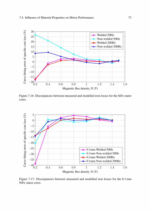
7.4. Influence of Material Properties on Motor Performance 73
0.2 0.4 0.6 0.8 1 1.2 1.4 1.6−20
−15
−10
−5
0
5
10
15
20
25
30
Magnetic flux density B (T)
Cur
vefi
ttin
ger
ror
ofsp
ecifi
cco
relo
ss(%
)
Welded 50HzNon-welded 50HzWelded 200HzNon-welded 200Hz
Figure 7.16: Discrepancies between measured and modelled iron losses for the SiFe statorcores.
0.2 0.4 0.6 0.8 1 1.2 1.4 1.6−40
−35
−30
−25
−20
−15
−10
−5
0
5
Magnetic flux density B (T)
Cur
vefi
ttin
ger
ror
ofsp
ecifi
cco
relo
ss(%
)
0.1mm Welded 50Hz0.1mm Non-welded 50Hz0.1mm Welded 200Hz0.1mm Non-welded 200Hz
Figure 7.17: Discrepancies between measured and modelled iron losses for the 0.1 mmNiFe stator cores.
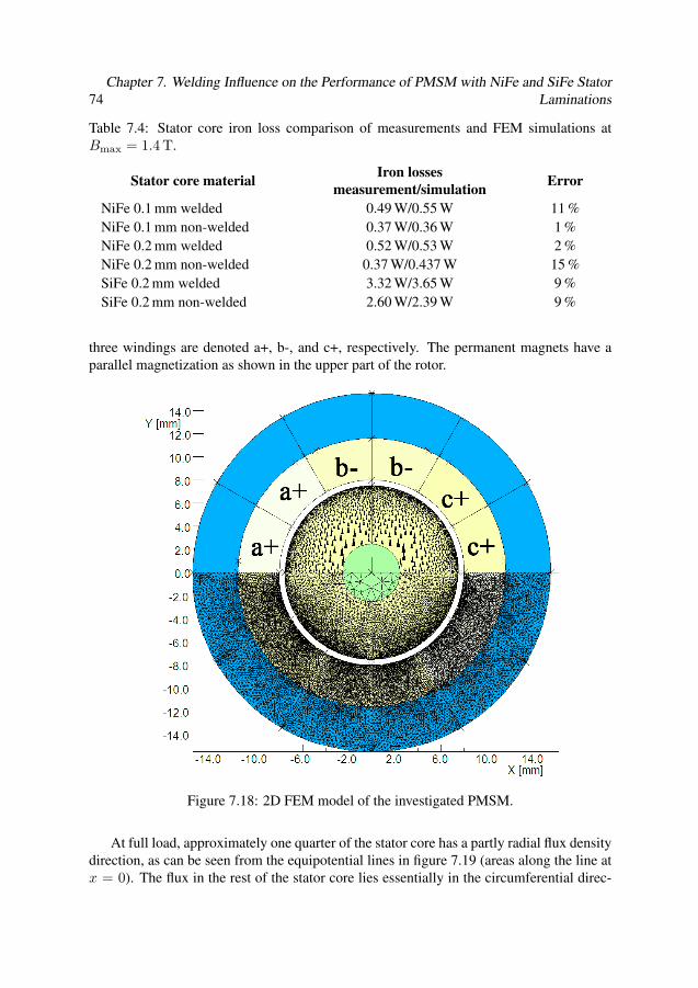
74Chapter 7. Welding Influence on the Performance of PMSM with NiFe and SiFe Stator
Laminations
Table 7.4: Stator core iron loss comparison of measurements and FEM simulations atBmax = 1.4 T.
Stator core materialIron losses
measurement/simulationError
NiFe 0.1 mm welded 0.49 W/0.55 W 11 %NiFe 0.1 mm non-welded 0.37 W/0.36 W 1 %NiFe 0.2 mm welded 0.52 W/0.53 W 2 %NiFe 0.2 mm non-welded 0.37 W/0.437 W 15 %SiFe 0.2 mm welded 3.32 W/3.65 W 9 %SiFe 0.2 mm non-welded 2.60 W/2.39 W 9 %
three windings are denoted a+, b-, and c+, respectively. The permanent magnets have aparallel magnetization as shown in the upper part of the rotor.
Figure 7.18: 2D FEM model of the investigated PMSM.
At full load, approximately one quarter of the stator core has a partly radial flux densitydirection, as can be seen from the equipotential lines in figure 7.19 (areas along the line atx = 0). The flux in the rest of the stator core lies essentially in the circumferential direc-
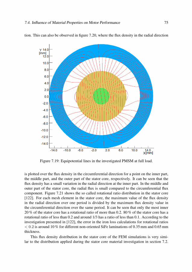
7.4. Influence of Material Properties on Motor Performance 75
tion. This can also be observed in figure 7.20, where the flux density in the radial direction
Figure 7.19: Equipotential lines in the investigated PMSM at full load.
is plotted over the flux density in the circumferential direction for a point on the inner part,the middle part, and the outer part of the stator core, respectively. It can be seen that theflux density has a small variation in the radial direction at the inner part. In the middle andouter part of the stator core, the radial flux is small compared to the circumferential fluxcomponent. Figure 7.21 shows the so called rotational ratio distribution in the stator core[122]. For each mesh element in the stator core, the maximum value of the flux densityin the radial direction over one period is divided by the maximum flux density value inthe circumferential direction over the same period. It can be seen that only the most inner20 % of the stator core has a rotational ratio of more than 0.2. 80 % of the stator core has arotational ratio of less than 0.2 and around 1/3 has a ratio of less than 0.1. According to theinvestigation presented in [122], the error in the iron loss calculations for rotational ratios< 0.2 is around 10 % for different non-oriented SiFe laminations of 0.35 mm and 0.65 mmthickness.
This flux density distribution in the stator core of the FEM simulations is very simi-lar to the distribution applied during the stator core material investigation in section 7.2.

76Chapter 7. Welding Influence on the Performance of PMSM with NiFe and SiFe Stator
Laminations
Table 7.5: Material influence of welded and non-welded stator cores on the back-emf peakvalue at no-load.
Stator core
materialBack-emf welded/non-welded
Voltage
reduction
NiFe 0.1 mm 60.09 V/60.57 V −1 %NiFe 0.2 mm 60.07 V/ 60.63 V −1 %SiFe 0.2 mm 60.02 V/60.57 V −1 %
Therefore, the experimental results are suitable to be used for the stator core material datain the FEM simulations.
−1.5 −1 −0.5 0 0.5 1 1.5−1.5
−1
−0.5
0
0.5
1
1.5
Magnetic flux density Bcircumferential (T)
Mag
neti
cfl
uxde
nsit
yB
rad
ial
(T)
Stator insideStator middleStator outside
Figure 7.20: Flux density in the stator core for the circumferential and radial direction atfull load.
The machine is simulated at a speed of 12 000 rpm, corresponding to an electrical fre-quency of 200 Hz. This is the largest frequency for which measured iron loss data is avail-able in section 7.2. The welding influence on the back-emf is shown in table 7.5 for theno-load case. This variation is very small. In order to investigate the torque and iron lossesfor the different core materials, the following simulations are conducted with a sinusoidalphase current with an amplitude of 15 A to keep the copper losses constant.
The torque results for the different materials are given in table 7.6. It can be seen thatthe change in torque is negligible small for the different stator cores (< 1 %). Due to the
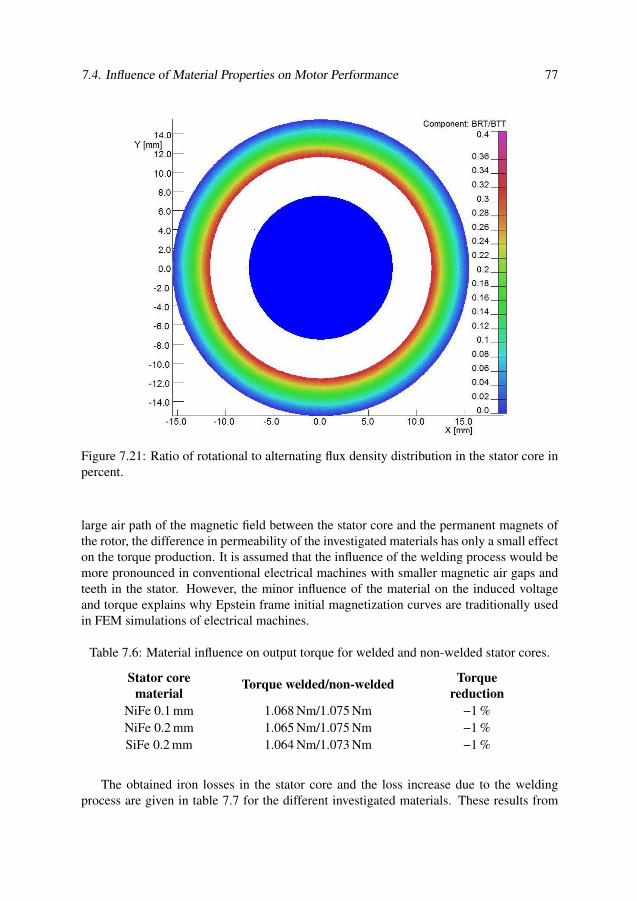
7.4. Influence of Material Properties on Motor Performance 77
Figure 7.21: Ratio of rotational to alternating flux density distribution in the stator core inpercent.
large air path of the magnetic field between the stator core and the permanent magnets ofthe rotor, the difference in permeability of the investigated materials has only a small effecton the torque production. It is assumed that the influence of the welding process would bemore pronounced in conventional electrical machines with smaller magnetic air gaps andteeth in the stator. However, the minor influence of the material on the induced voltageand torque explains why Epstein frame initial magnetization curves are traditionally usedin FEM simulations of electrical machines.
Table 7.6: Material influence on output torque for welded and non-welded stator cores.
Stator core
materialTorque welded/non-welded
Torque
reduction
NiFe 0.1 mm 1.068 Nm/1.075 Nm −1 %NiFe 0.2 mm 1.065 Nm/1.075 Nm −1 %SiFe 0.2 mm 1.064 Nm/1.073 Nm −1 %
The obtained iron losses in the stator core and the loss increase due to the weldingprocess are given in table 7.7 for the different investigated materials. These results from
78Chapter 7. Welding Influence on the Performance of PMSM with NiFe and SiFe Stator
Laminations
the FEM machine simulations are quite similar to the obtained loss increase of the coremeasurements given in table 7.3, especially for the NiFe stator cores. This emphasizesthe need to take into account the welding process influence on the stator lamination sheetswhen calculating iron losses in electrical machines. The results also show that it is possibleto decrease the iron losses for these operating points by 83 % and 76 % if the weldedSiFe stator cores are replaced by the welded NiFe stator cores with 0.1 mm and 0.2 mmlamination sheets, respectively.
Table 7.7: Material influence on iron losses for welded and non-welded stator cores at12 000 rpm.
Stator core material Iron losses welded/non-welded Loss increase
NiFe 0.1 mm 0.33 W/0.23 W +44 %NiFe 0.2 mm 0.46 W/0.34 W +35 %SiFe 0.2 mm 1.91 W/1.45 W +32 %
7.5 Conclusions
The influence of welding on the magnetic material properties and motor performance wasinvestigated for a slot-less permanent magnet synchronous machine. The studied magneticmaterials are affected differently by the welding process, both in terms of modifications ofthe BH hysteresis loops and the resulting iron losses. The magnetic property deteriorationof SiFe and NiFe electric steel sheets due to the manufacturing process of the stator corewas investigated.
The presented measurements give detailed results about the iron loss increase andchange of the magnetic BH hysteresis loop due to the stator core assembly. It is shownthat the cutting process of a small stator core and the welding step afterwards led to a sig-nificant change in the material properties, resulting in increased iron losses. This changecannot be predicted by Epstein frame measurements due to the neglected stator core ge-ometry and the non-existent welding seams. Regarding the change in iron losses due tothe welding process, it is shown that the NiFe cores are more strongly influenced by thewelding process than the SiFe cores, even though the latter ones have eight welding seamscompared to three for the NiFe cores.
Finally, it was shown, that the agreement between measurements and 3D FEM sim-ulations of ring core test specimen is satisfactory when iron losses are concerned. Thedeviation for the iron losses of the investigated stator cores is within 15 %. In addition,simulations of the considered PMSM show that the influence of the welding process onthe output torque is negligible. However, the simulations predict that the iron losses in thestator core may increase by 32 % to 44 % depending on the stator core material. Even withthe negative influence of the welding, changing the stator core material from SiFe to NiFewould still reduce the iron losses by more than 70 %.
Chapter 8
Thermal Influence on Magnetic
Properties and Performance of a PMSM
with NiFe Stator Laminations
Changes in the temperature of electrical machines influence amongst other things the
magnetic properties and iron losses. Usually iron losses decrease while winding losses
increase with increasing temperature [123]. The permeability due to magnetic domain
movements increases. But it is decreasing when it comes to magnetic domain rotations.
This behaviour leads in general to smaller magnetic saturation levels, as described in sec-
tion 5.1. This chapter investigates experimentally the temperature influences on the mag-
netic characteristics and iron losses for small stator cores of the slot-less PMSM which has
been introduced in the previous chapter. Including the thermal measurement results, FEM
simulations illustrate how the machine performance depends on the iron sheet temperature.
8.1 Investigated Stator Cores
The change in iron losses and magnetic properties is relatively small for SiFe steels, es-pecially for typical machine operation temperatures between 20 C to 100 C [124]. In-fluences for higher temperatures (up to 700 C) are investigated in [125] and [126]. It isshown that the saturation and permeability of SiFe is relatively stable for temperatures be-low 500 C and only changes significantly for temperatures above 600 C. Only the eddycurrent losses decrease slightly with increasing temperature due to the decreasing conduc-tivity of iron with the temperature. On the other hand, for NiFe laminations, temperaturesfor general machine operation (20 C to 100 C) already change the magnetic propertiesof the material noticeably. The temperature influence is thus only studied for three statorcores made of NiFe lamination sheets.
Two of the three cores are taken from the welding influencing study described in sec-tion 7.1. One has a lamination thickness of 0.1 mm and the other one has a thickness of0.2 mm. The third NiFe core has a lamination thickness of 0.2 mm and is from the same
79
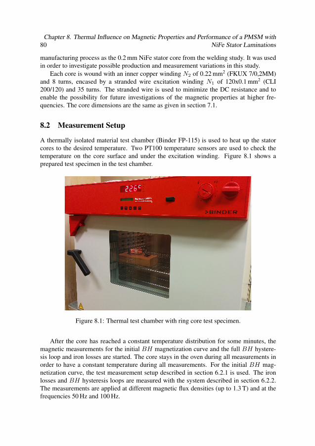
80Chapter 8. Thermal Influence on Magnetic Properties and Performance of a PMSM with
NiFe Stator Laminations
manufacturing process as the 0.2 mm NiFe stator core from the welding study. It was usedin order to investigate possible production and measurement variations in this study.
Each core is wound with an inner copper winding N2 of 0.22 mm2 (FKUX 7/0,2MM)and 8 turns, encased by a stranded wire excitation winding N1 of 120x0.1 mm2 (CLI200/120) and 35 turns. The stranded wire is used to minimize the DC resistance and toenable the possibility for future investigations of the magnetic properties at higher fre-quencies. The core dimensions are the same as given in section 7.1.
8.2 Measurement Setup
A thermally isolated material test chamber (Binder FP-115) is used to heat up the statorcores to the desired temperature. Two PT100 temperature sensors are used to check thetemperature on the core surface and under the excitation winding. Figure 8.1 shows aprepared test specimen in the test chamber.
Figure 8.1: Thermal test chamber with ring core test specimen.
After the core has reached a constant temperature distribution for some minutes, themagnetic measurements for the initial BH magnetization curve and the full BH hystere-sis loop and iron losses are started. The core stays in the oven during all measurements inorder to have a constant temperature during all measurements. For the initial BH mag-netization curve, the test measurement setup described in section 6.2.1 is used. The ironlosses and BH hysteresis loops are measured with the system described in section 6.2.2.The measurements are applied at different magnetic flux densities (up to 1.3 T) and at thefrequencies 50 Hz and 100 Hz.
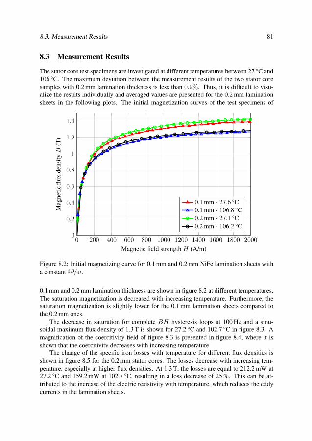
8.3. Measurement Results 81
8.3 Measurement Results
The stator core test specimens are investigated at different temperatures between 27 C and106 C. The maximum deviation between the measurement results of the two stator coresamples with 0.2 mm lamination thickness is less than 0.9%. Thus, it is difficult to visu-alize the results individually and averaged values are presented for the 0.2 mm laminationsheets in the following plots. The initial magnetization curves of the test specimens of
0 200 400 600 800 1000 1200 1400 1600 1800 20000
0.2
0.4
0.6
0.8
1
1.2
1.4
Magnetic field strength H (A/m)
Mag
neti
cfl
uxde
nsit
yB
(T)
0.1 mm - 27.6 C0.1 mm - 106.8 C0.2 mm - 27.1 C0.2 mm - 106.2 C
Figure 8.2: Initial magnetizing curve for 0.1 mm and 0.2 mm NiFe lamination sheets witha constant dB/dt.
0.1 mm and 0.2 mm lamination thickness are shown in figure 8.2 at different temperatures.The saturation magnetization is decreased with increasing temperature. Furthermore, thesaturation magnetization is slightly lower for the 0.1 mm lamination sheets compared tothe 0.2 mm ones.
The decrease in saturation for complete BH hysteresis loops at 100 Hz and a sinu-soidal maximum flux density of 1.3 T is shown for 27.2 C and 102.7 C in figure 8.3. Amagnification of the coercitivity field of figure 8.3 is presented in figure 8.4, where it isshown that the coercitivity decreases with increasing temperature.
The change of the specific iron losses with temperature for different flux densities isshown in figure 8.5 for the 0.2 mm stator cores. The losses decrease with increasing tem-perature, especially at higher flux densities. At 1.3 T, the losses are equal to 212.2 mW at27.2 C and 159.2 mW at 102.7 C, resulting in a loss decrease of 25 %. This can be at-tributed to the increase of the electric resistivity with temperature, which reduces the eddycurrents in the lamination sheets.

82Chapter 8. Thermal Influence on Magnetic Properties and Performance of a PMSM with
NiFe Stator Laminations
−3000 −2000 −1000 0 1000 2000 3000−1.5
−1
−0.5
0
0.5
1
1.5
Zoom
Magnetic field strength H (A/m)
Mag
neti
cfl
uxde
nsit
yB
(T)
27.2 C102.7 C
Figure 8.3: Complete BH hysteresis curves for 0.2 mm lamination sheets at 100 Hz and amaximum flux density of 1.3 T.
−40 −30 −20 −10 0 10 20 30 40−0.15
−0.1
−5 · 10−2
0
5 · 10−2
0.1
0.15
Magnetic field strength H (A/m)
Mag
neti
cfl
uxde
nsit
yB
(T)
27.2 C102.7 C
Figure 8.4: Zoom of the coercitivity field from figure 8.3.
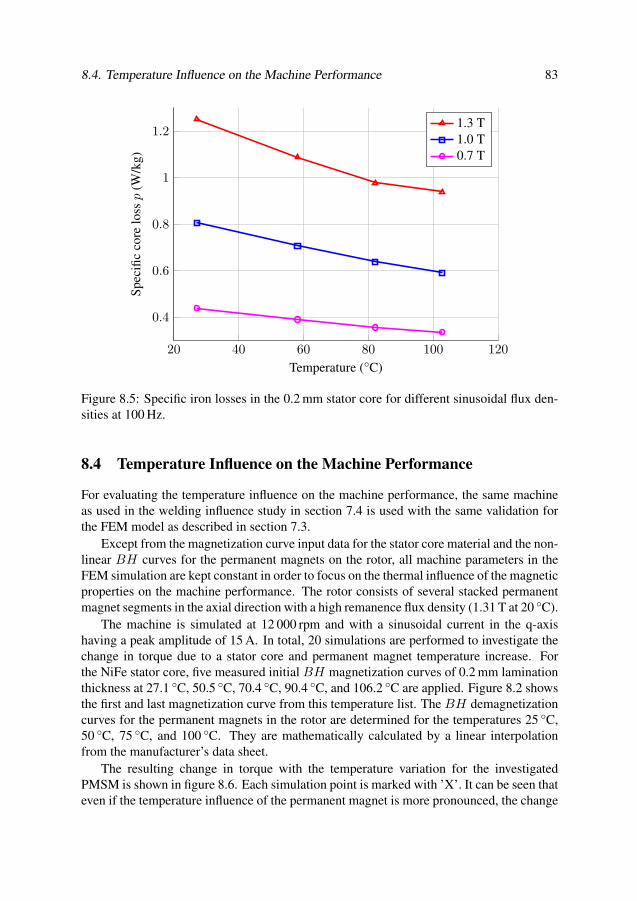
8.4. Temperature Influence on the Machine Performance 83
20 40 60 80 100 120
0.4
0.6
0.8
1
1.2
Temperature (C)
Spe
cifi
cco
relo
ssp
(W/k
g)1.3 T1.0 T0.7 T
Figure 8.5: Specific iron losses in the 0.2 mm stator core for different sinusoidal flux den-sities at 100 Hz.
8.4 Temperature Influence on the Machine Performance
For evaluating the temperature influence on the machine performance, the same machineas used in the welding influence study in section 7.4 is used with the same validation forthe FEM model as described in section 7.3.
Except from the magnetization curve input data for the stator core material and the non-linear BH curves for the permanent magnets on the rotor, all machine parameters in theFEM simulation are kept constant in order to focus on the thermal influence of the magneticproperties on the machine performance. The rotor consists of several stacked permanentmagnet segments in the axial direction with a high remanence flux density (1.31 T at 20 C).
The machine is simulated at 12 000 rpm and with a sinusoidal current in the q-axishaving a peak amplitude of 15 A. In total, 20 simulations are performed to investigate thechange in torque due to a stator core and permanent magnet temperature increase. Forthe NiFe stator core, five measured initial BH magnetization curves of 0.2 mm laminationthickness at 27.1 C, 50.5 C, 70.4 C, 90.4 C, and 106.2 C are applied. Figure 8.2 showsthe first and last magnetization curve from this temperature list. The BH demagnetizationcurves for the permanent magnets in the rotor are determined for the temperatures 25 C,50 C, 75 C, and 100 C. They are mathematically calculated by a linear interpolationfrom the manufacturer’s data sheet.
The resulting change in torque with the temperature variation for the investigatedPMSM is shown in figure 8.6. Each simulation point is marked with ’X’. It can be seen thateven if the temperature influence of the permanent magnet is more pronounced, the change

84Chapter 8. Thermal Influence on Magnetic Properties and Performance of a PMSM with
NiFe Stator Laminations
Permanent magnet temperature on rotor (C)
Sta
tor
core
tem
pera
ture
(C
)
1.2646
1.2397
1.2149
1.195
1.1702
Torque (Nm)
20 40 60 80 100 1.1
1.15
1.2
1.25
1.3
20
40
60
80
100
120
Figure 8.6: Electrical output torque of the PMSM as a function of on the stator core andpermanent magnet temperature (simulated points marked with ’X’).
Table 8.1: Temperature influence on output torque.
Stator
temperature
Magnet
temperatureTorque Rel. torque
27.1 C 25 C 1.27 Nm 100 %27.1 C 100 C 1.19 Nm 93.7 %
106.2 C 25 C 1.23 Nm 96.8 %106.2 C 100 C 1.16 Nm 91.3 %
of torque due to the temperature change in the stator core material is not negligible. Thetorque values at the minimum and maximum temperature of the stator core and permanentmagnet are also given in table 8.1. The output torque might decrease by almost 10% if themachine temperature increases from 25 C to 100 C.
The maximum torque of 1.27 Nm is obtained at the lowest temperatures (27.1 C forthe stator core and 25 C for the permanent magnets on the rotor), whereas the minimumtorque of 1.16 Nm is obtained at the highest temperatures (106.2 C and 100 C for thestator core and the permanent magnets, respectively). Out of the 8.7 % torque reduction,6.3 % are due to the reduced magnetization of the permanent magnets and nearly 2.4 % aredue to the reduced saturation level of the NiFe lamination.
The influence can be explained by the difference of the flux density in the stator core
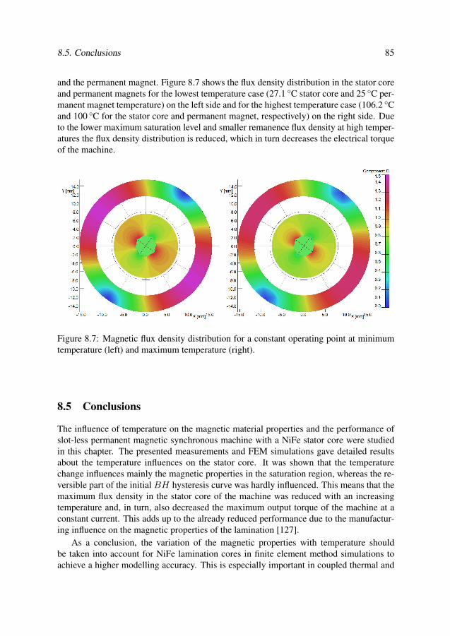
8.5. Conclusions 85
and the permanent magnet. Figure 8.7 shows the flux density distribution in the stator coreand permanent magnets for the lowest temperature case (27.1 C stator core and 25 C per-manent magnet temperature) on the left side and for the highest temperature case (106.2 Cand 100 C for the stator core and permanent magnet, respectively) on the right side. Dueto the lower maximum saturation level and smaller remanence flux density at high temper-atures the flux density distribution is reduced, which in turn decreases the electrical torqueof the machine.
Figure 8.7: Magnetic flux density distribution for a constant operating point at minimumtemperature (left) and maximum temperature (right).
8.5 Conclusions
The influence of temperature on the magnetic material properties and the performance ofslot-less permanent magnetic synchronous machine with a NiFe stator core were studiedin this chapter. The presented measurements and FEM simulations gave detailed resultsabout the temperature influences on the stator core. It was shown that the temperaturechange influences mainly the magnetic properties in the saturation region, whereas the re-versible part of the initial BH hysteresis curve was hardly influenced. This means that themaximum flux density in the stator core of the machine was reduced with an increasingtemperature and, in turn, also decreased the maximum output torque of the machine at aconstant current. This adds up to the already reduced performance due to the manufactur-ing influence on the magnetic properties of the lamination [127].
As a conclusion, the variation of the magnetic properties with temperature shouldbe taken into account for NiFe lamination cores in finite element method simulations toachieve a higher modelling accuracy. This is especially important in coupled thermal and
86Chapter 8. Thermal Influence on Magnetic Properties and Performance of a PMSM with
NiFe Stator Laminations
electromagnetic simulations, where the permanent magnet parameters are typically de-scribed as a function of the temperature.
Chapter 9
PWM Influence on Losses in SiFe and
NiFe Stator Laminations
In this chapter, the effects of distorted flux density waveforms in electrical machine stator
cores are studied. By using power electronics and inverters, the switched voltages extend
the harmonic spectrum of the local magnetic flux in an electrical machine. Consequently,
the iron losses are significantly influenced by the applied voltage switch patterns from in-
verters. The effects of pulse width modulation (PWM) inverters on the iron losses and
machine characteristics are studied for a small slot-less permanent magnet synchronous
machine supplied by a PWM voltage source inverter (VSI). Three different modulation
indices at different switching frequencies between 1 kHz and 20 kHz are studied experi-
mentally. Based on the measurement results, the influence of the time harmonics due to the
inverter switching schemes is investigated in FEM simulations to study the machine per-
formance. All measurements in this chapter are conducted with the measurement system
described in section 6.2.3.
9.1 Investigated Stator Cores
The influence of the PWM voltage switching is studied on the stator cores 1 to 4, whichwere also used in the welding influence investigations described in section 7.1 (see ta-ble 7.2). Two of the cores are made of SiFe lamination sheets and the other two of NiFelamination sheets, all with a lamination thickness of 0.2 mm. For each material two coresare taken out of the motor manufacturing process. One core is taken before and the otherone is retrieved after the welding step. The SiFe welded core has eight seams equallydistributed on the outer surface. The non-welded SiFe core is tightly pressed and heldtogether by a vinyl insulation tape. In the following they are referred to as “welded SiFecore” and “non-welded SiFe core”. The NiFe welded core has three welding seams equallydistributed on the outer core surface. The lamination sheets of the non-welded NiFe coreare glued together. These cores are referred to as “welded NiFe core” and “non-weldedNiFe core”, respectively.
87
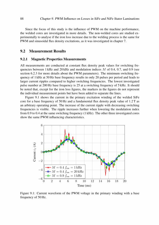
88 Chapter 9. PWM Influence on Losses in SiFe and NiFe Stator Laminations
Since the focus of this study is the influence of PWM on the machine performance,the welded cores are investigated in more details. The non-welded cores are studied ex-perimentally to analyse if the iron loss increase due to the welding process is the same forPWM and sinusoidal flux density excitations, as it was investigated in chapter 7.
9.2 Measurement Results
9.2.1 Magnetic Properties Measurements
All measurements are conducted at constant flux density peak values for switching fre-quencies between 1 kHz and 20 kHz and modulation indices M of 0.4, 0.7, and 0.9 (seesection 6.2.3 for more details about the PWM parameters). The minimum switching fre-quency of 1 kHz at 50 Hz base frequency results in only 20 pulses per period and leads tolarger current ripples compared to higher switching frequencies. The lowest investigatedpulse number at 200 Hz base frequency is 25 at a switching frequency of 5 kHz. It shouldbe noted that, except for the iron loss figures, the markers in the figures do not representthe individual measurement points but have been added to separate the lines.
Figure 9.1 shows the current in the primary excitation winding of the welded SiFecore for a base frequency of 50 Hz and a fundamental flux density peak value of 1.2 T asan arbitrary operating point. The increase of the current ripple with decreasing switchingfrequencies is visible. The ripple increases further when lowering the modulation indexfrom 0.9 to 0.4 at the same switching frequency (1 kHz). The other three investigated coresshow the same PWM influencing characteristics.
0 2 4 6 8 10 12 14 16 18 20−6
−4
−2
0
2
4
6
Time (ms)
Cur
rent
i 1(A
)
M = 0.4 fsw = 1 kHzM = 0.4 fsw = 20 kHzM = 0.9 fsw = 1 kHz
Figure 9.1: Current waveform of the PWM voltage in the primary winding with a basefrequency of 50 Hz.
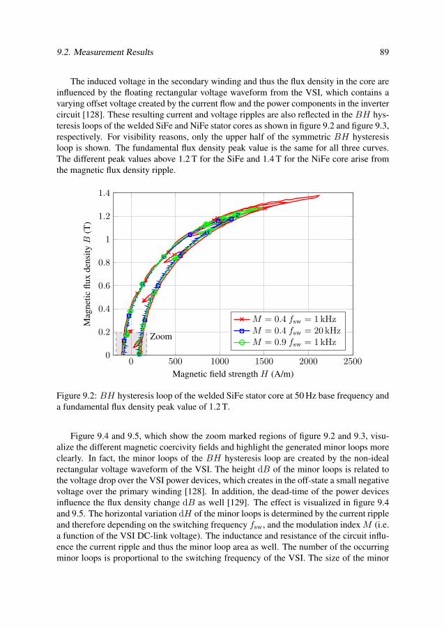
9.2. Measurement Results 89
The induced voltage in the secondary winding and thus the flux density in the core areinfluenced by the floating rectangular voltage waveform from the VSI, which contains avarying offset voltage created by the current flow and the power components in the invertercircuit [128]. These resulting current and voltage ripples are also reflected in the BH hys-teresis loops of the welded SiFe and NiFe stator cores as shown in figure 9.2 and figure 9.3,respectively. For visibility reasons, only the upper half of the symmetric BH hysteresisloop is shown. The fundamental flux density peak value is the same for all three curves.The different peak values above 1.2 T for the SiFe and 1.4 T for the NiFe core arise fromthe magnetic flux density ripple.
0 500 1000 1500 2000 25000
0.2
0.4
0.6
0.8
1
1.2
1.4
Zoom
Magnetic field strength H (A/m)
Mag
neti
cfl
uxde
nsit
yB
(T)
M = 0.4 fsw = 1 kHzM = 0.4 fsw = 20 kHzM = 0.9 fsw = 1 kHz
Figure 9.2: BH hysteresis loop of the welded SiFe stator core at 50 Hz base frequency anda fundamental flux density peak value of 1.2 T.
Figure 9.4 and 9.5, which show the zoom marked regions of figure 9.2 and 9.3, visu-alize the different magnetic coercivity fields and highlight the generated minor loops moreclearly. In fact, the minor loops of the BH hysteresis loop are created by the non-idealrectangular voltage waveform of the VSI. The height dB of the minor loops is related tothe voltage drop over the VSI power devices, which creates in the off-state a small negativevoltage over the primary winding [128]. In addition, the dead-time of the power devicesinfluence the flux density change dB as well [129]. The effect is visualized in figure 9.4and 9.5. The horizontal variation dH of the minor loops is determined by the current rippleand therefore depending on the switching frequency fsw, and the modulation index M (i.e.a function of the VSI DC-link voltage). The inductance and resistance of the circuit influ-ence the current ripple and thus the minor loop area as well. The number of the occurringminor loops is proportional to the switching frequency of the VSI. The size of the minor
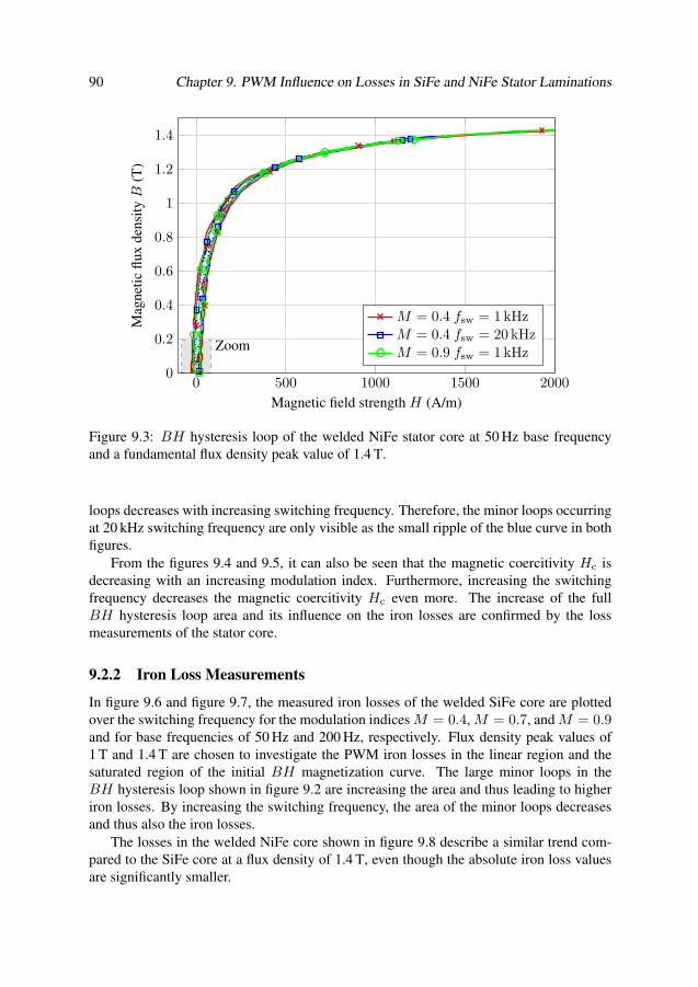
90 Chapter 9. PWM Influence on Losses in SiFe and NiFe Stator Laminations
0 500 1000 1500 20000
0.2
0.4
0.6
0.8
1
1.2
1.4
Zoom
Magnetic field strength H (A/m)
Mag
neti
cfl
uxde
nsit
yB
(T)
M = 0.4 fsw = 1 kHzM = 0.4 fsw = 20 kHzM = 0.9 fsw = 1 kHz
Figure 9.3: BH hysteresis loop of the welded NiFe stator core at 50 Hz base frequencyand a fundamental flux density peak value of 1.4 T.
loops decreases with increasing switching frequency. Therefore, the minor loops occurringat 20 kHz switching frequency are only visible as the small ripple of the blue curve in bothfigures.
From the figures 9.4 and 9.5, it can also be seen that the magnetic coercitivity Hc isdecreasing with an increasing modulation index. Furthermore, increasing the switchingfrequency decreases the magnetic coercitivity Hc even more. The increase of the fullBH hysteresis loop area and its influence on the iron losses are confirmed by the lossmeasurements of the stator core.
9.2.2 Iron Loss Measurements
In figure 9.6 and figure 9.7, the measured iron losses of the welded SiFe core are plottedover the switching frequency for the modulation indices M = 0.4, M = 0.7, and M = 0.9and for base frequencies of 50 Hz and 200 Hz, respectively. Flux density peak values of1 T and 1.4 T are chosen to investigate the PWM iron losses in the linear region and thesaturated region of the initial BH magnetization curve. The large minor loops in theBH hysteresis loop shown in figure 9.2 are increasing the area and thus leading to higheriron losses. By increasing the switching frequency, the area of the minor loops decreasesand thus also the iron losses.
The losses in the welded NiFe core shown in figure 9.8 describe a similar trend com-pared to the SiFe core at a flux density of 1.4 T, even though the absolute iron loss valuesare significantly smaller.

9.2. Measurement Results 91
−150 −100 −50 0 50 100 150−0.2
−0.1
0
0.1
0.2
dH
dB
Magnetic field strength H (A/m)
Mag
neti
cfl
uxde
nsit
yB
(T)
M = 0.4 fsw = 1 kHzM = 0.4 fsw = 20 kHzM = 0.9 fsw = 1 kHz
Figure 9.4: Magnification of the welded SiFe BH hysteresis loop from figure 9.2 aroundzero flux density (grey rectangle).
−60 −40 −20 0 20 40 60−0.2
−0.1
0
0.1
0.2
dH
dB
Magnetic field strength H (A/m)
Mag
neti
cfl
uxde
nsit
yB
(T)
M = 0.4 fsw = 1 kHzM = 0.4 fsw = 20 kHzM = 0.9 fsw = 1 kHz
Figure 9.5: Magnification of the welded NiFe BH hysteresis loop from figure 9.3 aroundzero flux density (grey rectangle).

92 Chapter 9. PWM Influence on Losses in SiFe and NiFe Stator Laminations
0 5 10 15 202
3
4
5
6
7
Switching frequency fsw (kHz)
Spe
cifi
cco
relo
ssp
(W/k
g)M = 0.4 B = 1.4 TM = 0.7 B = 1.4 TM = 0.9 B = 1.4 TM = 0.4 B = 1 TM = 0.7 B = 1 TM = 0.9 B = 1 T
Figure 9.6: Iron losses in the welded SiFe stator core at a base frequency of 50 Hz andfundamental flux density peak values of 1 T and 1.4 T, respectively.
5 10 15 20
10
20
30
40
Switching frequency fsw (kHz)
Spe
cifi
cco
relo
ssp
(W/k
g)
M = 0.4 B = 1.4 TM = 0.7 B = 1.4 TM = 0.9 B = 1.4 TM = 0.4 B = 1 TM = 0.7 B = 1 TM = 0.9 B = 1 T
Figure 9.7: Iron losses in the welded SiFe stator core at a base frequency of 200 Hz and afundamental flux density peak value of 1 T and 1.4 T, respectively.
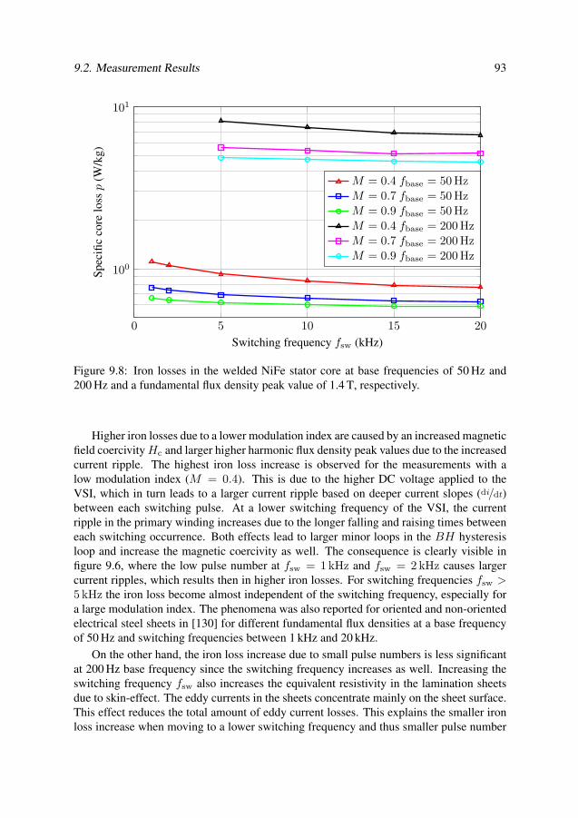
9.2. Measurement Results 93
0 5 10 15 20
100
101
Switching frequency fsw (kHz)
Spe
cifi
cco
relo
ssp
(W/k
g)
M = 0.4 fbase = 50 HzM = 0.7 fbase = 50 HzM = 0.9 fbase = 50 HzM = 0.4 fbase = 200 HzM = 0.7 fbase = 200 HzM = 0.9 fbase = 200 Hz
Figure 9.8: Iron losses in the welded NiFe stator core at base frequencies of 50 Hz and200 Hz and a fundamental flux density peak value of 1.4 T, respectively.
Higher iron losses due to a lower modulation index are caused by an increased magneticfield coercivity Hc and larger higher harmonic flux density peak values due to the increasedcurrent ripple. The highest iron loss increase is observed for the measurements with alow modulation index (M = 0.4). This is due to the higher DC voltage applied to theVSI, which in turn leads to a larger current ripple based on deeper current slopes (di/dt)between each switching pulse. At a lower switching frequency of the VSI, the currentripple in the primary winding increases due to the longer falling and raising times betweeneach switching occurrence. Both effects lead to larger minor loops in the BH hysteresisloop and increase the magnetic coercivity as well. The consequence is clearly visible infigure 9.6, where the low pulse number at fsw = 1 kHz and fsw = 2 kHz causes largercurrent ripples, which results then in higher iron losses. For switching frequencies fsw >5 kHz the iron loss become almost independent of the switching frequency, especially fora large modulation index. The phenomena was also reported for oriented and non-orientedelectrical steel sheets in [130] for different fundamental flux densities at a base frequencyof 50 Hz and switching frequencies between 1 kHz and 20 kHz.
On the other hand, the iron loss increase due to small pulse numbers is less significantat 200 Hz base frequency since the switching frequency increases as well. Increasing theswitching frequency fsw also increases the equivalent resistivity in the lamination sheetsdue to skin-effect. The eddy currents in the sheets concentrate mainly on the sheet surface.This effect reduces the total amount of eddy current losses. This explains the smaller ironloss increase when moving to a lower switching frequency and thus smaller pulse number

94 Chapter 9. PWM Influence on Losses in SiFe and NiFe Stator Laminations
in figure 9.7. However, the trend of the iron loss change with the switching frequency at agiven modulation index is similar for the investigated flux density peak values of 1 T and1.4 T at both base frequencies.
For investigating the VSI switching effect on the iron losses, the results from figure 9.6,figure 9.7, and figure 9.8 are compared to the iron loss measurement results with a sinu-soidal flux density waveform, as specified by the IEC standard 60404-6 [28] and presentedin section 7.2. The results are shown in figure 9.9 and figure 9.10 for the welded SiFe core
0 5 10 15 200
20
40
60
80
Switching frequency fsw (kHz)
Spe
cifi
cco
relo
ssin
crea
se(%
)
M = 0.4 B = 1.4 TM = 0.4 B = 1 TM = 0.7 B = 1.4 TM = 0.7 B = 1 TM = 0.9 B = 1.4 TM = 0.9 B = 1 T
Figure 9.9: Iron loss increase (PWM/sinusoidal) in the welded SiFe stator core at a basefrequency of 50 Hz related to pure sinusoidal flux density iron losses.
at 50 Hz and 200 Hz, and in figure 9.11 for the welded NiFe core at a flux density of 1.4 T,respectively.
The most significant iron loss increase is for both welded cores at 50 Hz base frequencyand in the case of a low modulation index and low switching frequencies. For the weldedSiFe core, the iron losses increase by up to 80 % and for the welded NiFe core increases ofmore than 100 % are reached at a modulation index of 0.4. This significant loss increaseis due to the large current ripple caused by the high DC-link voltage required at low mod-ulation indices, as it was shown in figure 9.1. By selecting higher switching frequenciesand a better utilization of the DC-link voltage (higher modulation index M ), the iron lossincrease due to the VSI can be reduced to between 10 % to 20 %. With increasing switch-ing frequency, the current ripple reduces considerably and thus also the iron losses. Forswitching frequencies larger than 15 kHz (SiFe core) and 5 kHz (NiFe core) and a modula-tion index of 0.9, the iron loss increase is almost constant for both base frequencies (50 Hzand 200 Hz). The in average higher iron loss increase for the welded NiFe stator core,especially at 200 Hz base frequency, might be due to the fact that the welded NiFe stator
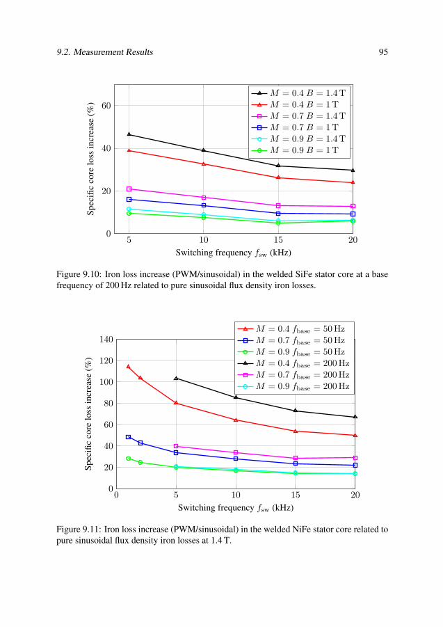
9.2. Measurement Results 95
5 10 15 200
20
40
60
Switching frequency fsw (kHz)
Spe
cifi
cco
relo
ssin
crea
se(%
)M = 0.4 B = 1.4 TM = 0.4 B = 1 TM = 0.7 B = 1.4 TM = 0.7 B = 1 TM = 0.9 B = 1.4 TM = 0.9 B = 1 T
Figure 9.10: Iron loss increase (PWM/sinusoidal) in the welded SiFe stator core at a basefrequency of 200 Hz related to pure sinusoidal flux density iron losses.
0 5 10 15 200
20
40
60
80
100
120
140
Switching frequency fsw (kHz)
Spe
cifi
cco
relo
ssin
crea
se(%
)
M = 0.4 fbase = 50 HzM = 0.7 fbase = 50 HzM = 0.9 fbase = 50 HzM = 0.4 fbase = 200 HzM = 0.7 fbase = 200 HzM = 0.9 fbase = 200 Hz
Figure 9.11: Iron loss increase (PWM/sinusoidal) in the welded NiFe stator core related topure sinusoidal flux density iron losses at 1.4 T.

96 Chapter 9. PWM Influence on Losses in SiFe and NiFe Stator Laminations
core is higher saturated at 1.4 T and thus has a lower permeability in this region comparedto the welded SiFe core.
The influence of the manufacturing welding process is investigated by comparing thewelded and the non-welded stator core iron losses at the base frequencies of 50 Hz and200 Hz for the SiFe core and at 50 Hz for the NiFe core, as shown in figure 9.12.
0 5 10 15 200
5
10
15
20
25
30
35
40
45
Switching frequency fsw (kHz)
Spe
cifi
cco
relo
ssin
crea
se(%
)
SiFe M = 0.4 fbase = 50 HzSiFe M = 0.7 fbase = 50 HzSiFe M = 0.9 fbase = 50 HzSiFe M = 0.4 fbase = 200 HzSiFe M = 0.7 fbase = 200 HzSiFe M = 0.9 fbase = 200 HzNiFe M = 0.4 fbase = 50 HzNiFe M = 0.7 fbase = 50 HzNiFe M = 0.9 fbase = 50 Hz
Figure 9.12: Relative core loss increase between the welded and non-welded SiFe andNiFe stator cores at different modulation indices and a magnetic flux density peak value of1.4 T.
For both materials, the relative core loss increase is the lowest for small modulationindices, since their absolute loss values are already the largest. The loss increase at themodulation indices M of 0.7 and 0.9 is almost the same for all cases and relatively inde-pendent of the switching frequency. The fact that the relative core loss increase betweenthe welded and non-welded SiFe core is larger at 50 Hz compared to 200 Hz can be at-tributed to the significant larger amount of absolute iron losses at 200 Hz, so that the lossincrease of almost 3.5 W/kg is less significant than the absolute loss increase at 50 Hz,which is between 0.8 W/kg and 1.1 W/kg. As also shown before in the welding influencestudy with sinusoidal flux density values (section 7.2), the NiFe cores are more influencedby the welding process compared to the SiFe cores. In both studies, the iron loss increasefor the NiFe cores after the welding process is around 40 % (pure sinusoidal excitation andfor modulation indices M of 0.7 and 0.9). For the SiFe cores, the percentage of iron lossincrease due to the welding process is slightly larger for the higher modulation indices of0.7 and 0.9 compared to the pure sinusoidal flux density excitation presented in section 7.2.Finally, the results show that the iron loss increase is almost independent of the switchingfrequency if it is larger than 5 kHz.
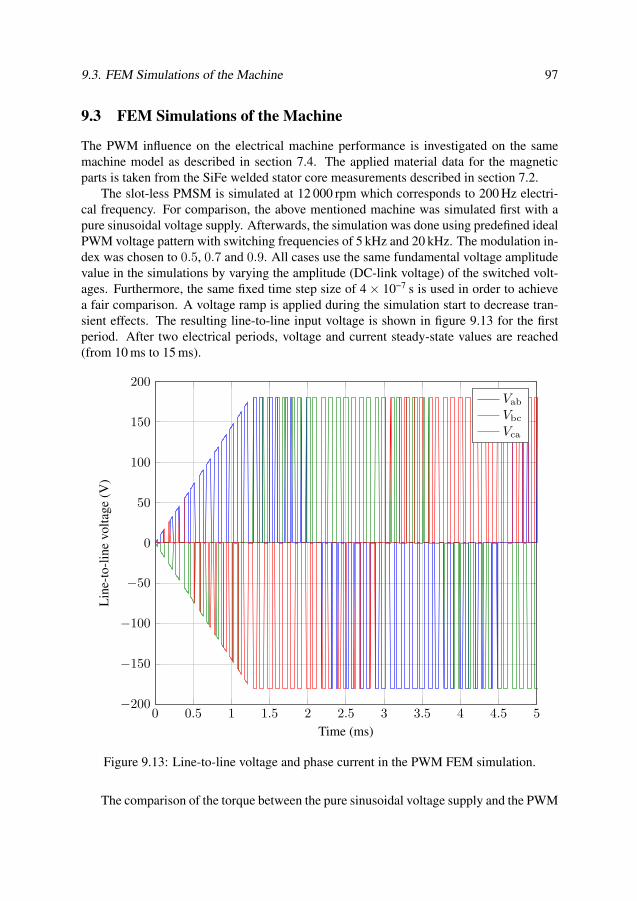
9.3. FEM Simulations of the Machine 97
9.3 FEM Simulations of the Machine
The PWM influence on the electrical machine performance is investigated on the samemachine model as described in section 7.4. The applied material data for the magneticparts is taken from the SiFe welded stator core measurements described in section 7.2.
The slot-less PMSM is simulated at 12 000 rpm which corresponds to 200 Hz electri-cal frequency. For comparison, the above mentioned machine was simulated first with apure sinusoidal voltage supply. Afterwards, the simulation was done using predefined idealPWM voltage pattern with switching frequencies of 5 kHz and 20 kHz. The modulation in-dex was chosen to 0.5, 0.7 and 0.9. All cases use the same fundamental voltage amplitudevalue in the simulations by varying the amplitude (DC-link voltage) of the switched volt-ages. Furthermore, the same fixed time step size of 4 × 10⁻⁷ s is used in order to achievea fair comparison. A voltage ramp is applied during the simulation start to decrease tran-sient effects. The resulting line-to-line input voltage is shown in figure 9.13 for the firstperiod. After two electrical periods, voltage and current steady-state values are reached(from 10 ms to 15 ms).
0 0.5 1 1.5 2 2.5 3 3.5 4 4.5 5−200
−150
−100
−50
0
50
100
150
200
Time (ms)
Lin
e-to
-lin
evo
ltag
e(V
)
Vab
Vbc
Vca
Figure 9.13: Line-to-line voltage and phase current in the PWM FEM simulation.
The comparison of the torque between the pure sinusoidal voltage supply and the PWM

98 Chapter 9. PWM Influence on Losses in SiFe and NiFe Stator Laminations
voltage source with a switching frequency of 20 kHz and 0.9 modulation index is shown infigure 9.14 for the first three periods. Since the fundamental voltage is the same for bothsimulations, the fundamental torque is also matching. This demonstrates the correctnessof the FEM simulations in terms of initial phase angle and a correct fundamental excita-tion voltage, respectively. The clearly visible torque ripple of the PWM signal shows theinfluence on the machine output torque due to the voltage switching.
Figure 9.15 shows the third period of the torque simulation in figure 9.14. For thePWM voltage signal, the high-frequency torque ripple due to the PWM operation is clearlyvisible, as well as the low-frequency ripple due to the three phase machine operation (6pulses per period). For the sinusoidal operation, the low-frequency torque ripple is notrecognizable in this scale due to the slot-less stator core and its resulting large inductance.
0 2 4 6 8 10 12 14 16−2
−1
0
1
Time (ms)
Tor
que
(Nm
)
M = 0.9 fsw = 20 kHzpure sinusoidal
Figure 9.14: Torque comparison between PWM and sinusoidal voltage excitation.
A torque ripple comparison for 5 kHz and 20 kHz switching frequency with a fixedmodulation index of 0.9 is shown in figure 9.16. The torque ripple at 5 kHz switchingfrequency is around 25 %, whereas for a switching frequency of 20 kHz it is only 7 %.The difference in torque ripple is smaller for different modulation indices at a constantswitching frequency. For a switching frequency of 5 kHz and a modulation index of 0.5the torque ripple becomes 31 %, an increase by 6 %, as can be seen in figure 9.17.
Comparing the flux density distribution in the stator core for an arbitrary operationalpoint does not show a distinguishable difference between the sinusoidal and different PWMexcitation simulations. However, an analysis of the harmonic content of the flux densitydistribution in each FEM element of the stator discloses the difference between the si-nusoidal and PWM excitation cases. In the PWM simulations with 5 kHz switching fre-quency, noticeable flux density amplitudes were found for the 23rd and 27th harmonic, as
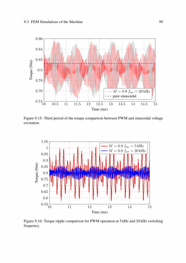
9.3. FEM Simulations of the Machine 99
10 10.5 11 11.5 12 12.5 13 13.5 14 14.5 150.74
0.76
0.78
0.8
0.82
0.84
0.86
Time (ms)
Tor
que
(Nm
)
M = 0.9 fsw = 20 kHzpure sinusoidal
Figure 9.15: Third period of the torque comparison between PWM and sinusoidal voltageexcitation.
10 11 12 13 14 150.55
0.6
0.65
0.7
0.75
0.8
0.85
0.9
0.95
1
1.05
Time (ms)
Tor
que
(Nm
)
M = 0.9 fsw = 5 kHzM = 0.9 fsw = 20 kHz
Figure 9.16: Torque ripple comparison for PWM operation at 5 kHz and 20 kHz switchingfrequency.

100 Chapter 9. PWM Influence on Losses in SiFe and NiFe Stator Laminations
10 10.5 11 11.5 12 12.5 13 13.5 14 14.5 15
0.6
0.8
1
1.2
Time (ms)
Tor
que
(Nm
)
M = 0.5 fsw = 5 kHzM = 0.9 fsw = 5 kHz
Figure 9.17: Torque ripple comparison for PWM operation at modulation indices of 0.5and 0.9 at 5 kHz switching frequency.
it is shown for the 23rd harmonic in figure 9.18. This can be explained by the PWM pulsenumber of 5 kHz/200 Hz = 25. Similar flux density amplitudes were found around the 100thharmonic for a base frequency of 200 Hz.
The influence of the higher harmonic flux densities is also reflected in the iron losses.In section 7.3, it was shown that the flux density distribution in the stator core of theFEM simulations is very similar to the distribution applied during the stator core materialmeasurements. Therefore, it is assumed to be valid to use previously determined iron lossparameters from sinusoidal excitation studies also for estimating the iron loss increase dueto the PWM switching effects.
The iron losses in the stator core are determined with the loss separation approach of(4.12) presented in section 4.3. In the Opera FEM software, the harmonic components ofthe flux density in each element are taken into account in the loss separation approach withthe following equation [66]:
PFe =∑
h
ChysthfBαh + Cec(hf)2B2
h + Cexc(hf)1.5B1.5h . (9.1)
In (9.1), h refers to the harmonic order. In the following iron loss studies, the losseswere calculated up to the 212th harmonic. The variables Chyst, Cec, Cexc and α are fittingcoefficients which are derived from sinusoidal excitation iron loss measurements for thehysteresis, eddy current and excess losses, respectively. The same values as described inmore detail in section 7.4 were chosen.
The iron losses for different modulation indices at the switching frequencies 5 kHzand 20 kHz are shown in figure 9.19. At a constant fundamental voltage excitation the
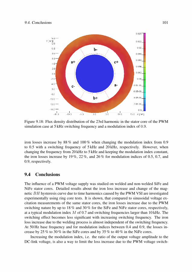
9.4. Conclusions 101
Figure 9.18: Flux density distribution of the 23rd harmonic in the stator core of the PWMsimulation case at 5 kHz switching frequency and a modulation index of 0.9.
iron losses increase by 88 % and 100 % when changing the modulation index from 0.9to 0.5 with a switching frequency of 5 kHz and 20 kHz, respectively. However, whenchanging the frequency from 20 kHz to 5 kHz and keeping the modulation index constant,the iron losses increase by 19 %, 22 %, and 26 % for modulation indices of 0.5, 0.7, and0.9, respectively.
9.4 Conclusions
The influence of a PWM voltage supply was studied on welded and non-welded SiFe andNiFe stator cores. Detailed results about the iron loss increase and change of the mag-netic BH hysteresis curve due to time harmonics caused by the PWM VSI are investigatedexperimentally using ring core tests. It is shown, that compared to sinusoidal voltage ex-citation measurements of the same stator cores, the iron losses increase due to the PWMswitching nature by up to 18 % and 30 % for the SiFe and NiFe stator cores, respectively,at a typical modulation index M of 0.7 and switching frequencies larger than 10 kHz. Theswitching effect becomes less significant with increasing switching frequency. The ironloss increase due to the welding process is almost independent of the switching frequency.At 50 Hz base frequency and for modulation indices between 0.4 and 0.9, the losses in-crease by 25 % to 30 % in the SiFe cores and by 35 % to 40 % in the NiFe cores.
Increasing the modulation index, i.e. the ratio of the output voltage amplitude to theDC-link voltage, is also a way to limit the loss increase due to the PWM voltage switch-
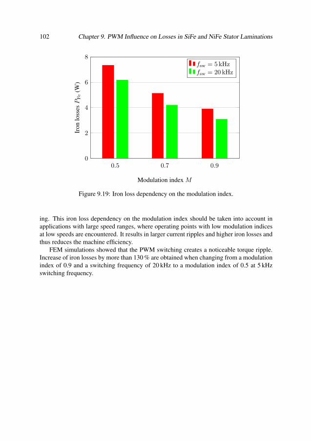
102 Chapter 9. PWM Influence on Losses in SiFe and NiFe Stator Laminations
0.5 0.7 0.90
2
4
6
8
0.5 0.7 0.90
2
4
6
8
Modulation index M
Iron
loss
esP
Fe
(W)
fsw = 5 kHzfsw = 20 kHz
Figure 9.19: Iron loss dependency on the modulation index.
ing. This iron loss dependency on the modulation index should be taken into account inapplications with large speed ranges, where operating points with low modulation indicesat low speeds are encountered. It results in larger current ripples and higher iron losses andthus reduces the machine efficiency.
FEM simulations showed that the PWM switching creates a noticeable torque ripple.Increase of iron losses by more than 130 % are obtained when changing from a modulationindex of 0.9 and a switching frequency of 20 kHz to a modulation index of 0.5 at 5 kHzswitching frequency.

Chapter 10
Annealing Influence on Magnetic
Properties of NiFe and CoFe Stator
Laminations
Cobalt-iron (CoFe) and nickel-iron (NiFe) are from a physical point of view ideal mag-
netic material alloys for electrical machines, as it was discussed in chapter 5. However,
these alloys are relatively sensitive to mechanical and thermal stress. Therefore, a heat
treatment after the cutting or punching process, generally and also in the following called
annealing, is indispensable in order to achieve the desired magnetic characteristics for a
certain application. In this chapter, the influence of the annealing process on the magnetic
properties is studied for a CoFe stator core of a permanent magnet synchronous generator
and for a NiFe stator core of a small slot-less permanent magnet synchronous machine.
Magnetic ring core measurements are applied on the stator cores. Furthermore, the ma-
terial samples are investigated with microscopic analyses to determine the change of the
grain structure due to the annealing process.
10.1 Investigated Stator Cores
In the CoFe alloy study, three stator core samples are investigated by magnetic stator yokemeasurements and a microscopic analysis. The CoFe lamination material of the statorcores is 0.35 mm thick and made of 49% cobalt, 49% iron, and 2% vanadium (all weight%). The laminations are complying with alloy class F11 (IEC 60404-8-6) [131]. SampleA is a stator core from before the annealing process. The lamination sheets are stackedand tightly held together by plastic strips. The stator laminations of sample B and C wereannealed after the cutting process in a hydrogen atmosphere at 760 C for 2 hours and at850 C for 3 hours, respectively. Afterwards they were as well stacked together to form sta-tor cores and fixed by plastic strips. Table 10.1 gives an overview of the CoFe stator cores.The study on the CoFe material was carried out at the Energy Department of Politecnicodi Torino, Italy, in collaboration with the PhD student Marco Cossale.
103
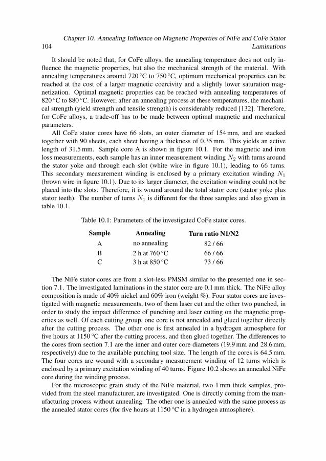
104Chapter 10. Annealing Influence on Magnetic Properties of NiFe and CoFe Stator
Laminations
It should be noted that, for CoFe alloys, the annealing temperature does not only in-fluence the magnetic properties, but also the mechanical strength of the material. Withannealing temperatures around 720 C to 750 C, optimum mechanical properties can bereached at the cost of a larger magnetic coercivity and a slightly lower saturation mag-netization. Optimal magnetic properties can be reached with annealing temperatures of820 C to 880 C. However, after an annealing process at these temperatures, the mechani-cal strength (yield strength and tensile strength) is considerably reduced [132]. Therefore,for CoFe alloys, a trade-off has to be made between optimal magnetic and mechanicalparameters.
All CoFe stator cores have 66 slots, an outer diameter of 154 mm, and are stackedtogether with 90 sheets, each sheet having a thickness of 0.35 mm. This yields an activelength of 31.5 mm. Sample core A is shown in figure 10.1. For the magnetic and ironloss measurements, each sample has an inner measurement winding N2 with turns aroundthe stator yoke and through each slot (white wire in figure 10.1), leading to 66 turns.This secondary measurement winding is enclosed by a primary excitation winding N1
(brown wire in figure 10.1). Due to its larger diameter, the excitation winding could not beplaced into the slots. Therefore, it is wound around the total stator core (stator yoke plusstator teeth). The number of turns N1 is different for the three samples and also given intable 10.1.
Table 10.1: Parameters of the investigated CoFe stator cores.
Sample Annealing Turn ratio N1/N2
A no annealing 82 / 66
B 2 h at 760 C 66 / 66C 3 h at 850 C 73 / 66
The NiFe stator cores are from a slot-less PMSM similar to the presented one in sec-tion 7.1. The investigated laminations in the stator core are 0.1 mm thick. The NiFe alloycomposition is made of 40% nickel and 60% iron (weight %). Four stator cores are inves-tigated with magnetic measurements, two of them laser cut and the other two punched, inorder to study the impact difference of punching and laser cutting on the magnetic prop-erties as well. Of each cutting group, one core is not annealed and glued together directlyafter the cutting process. The other one is first annealed in a hydrogen atmosphere forfive hours at 1150 C after the cutting process, and then glued together. The differences tothe cores from section 7.1 are the inner and outer core diameters (19.9 mm and 28.6 mm,respectively) due to the available punching tool size. The length of the cores is 64.5 mm.The four cores are wound with a secondary measurement winding of 12 turns which isenclosed by a primary excitation winding of 40 turns. Figure 10.2 shows an annealed NiFecore during the winding process.
For the microscopic grain study of the NiFe material, two 1 mm thick samples, pro-vided from the steel manufacturer, are investigated. One is directly coming from the man-ufacturing process without annealing. The other one is annealed with the same process asthe annealed stator cores (for five hours at 1150 C in a hydrogen atmosphere).
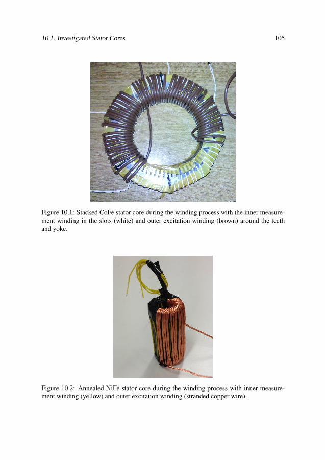
10.1. Investigated Stator Cores 105
Figure 10.1: Stacked CoFe stator core during the winding process with the inner measure-ment winding in the slots (white) and outer excitation winding (brown) around the teethand yoke.
Figure 10.2: Annealed NiFe stator core during the winding process with inner measure-ment winding (yellow) and outer excitation winding (stranded copper wire).
106Chapter 10. Annealing Influence on Magnetic Properties of NiFe and CoFe Stator
Laminations
10.2 Microscopic Analysis
With the microscopic analysis, it is possible to study the crystallographic grain structureof the material. As discussed in section 5.1, the magnetization of ferromagnetic materialsare heavily depending on the magnetic domains, which are related to the grain structure ofthe ferromagnetic material. Larger grains are in general an indication for better magneticproperties in terms of saturation magnetization and magnetic coercivity. The microscopicinvestigation of the CoFe alloy was done at the material science group of the Energy De-partment of Politecnico di Torino in Italy. The NiFe alloy samples were investigated bySwerea KIMAB AB in Sweden.
For CoFe, the lamination sheets from the stators A, B and C were evaluated by an op-tical microscopic analysis to investigate the change of the crystallographic grain structurebefore and after the annealing process. The short side (0.35 mm) as well as the middle ofthe surface were analysed. Figure 10.3 shows the material structure at the short 0.35 mmside of the sheets at 500x magnification and figure 10.4 the surface plane of the sheetsat 200x magnification. Before the annealing process, no real grain structure is recogniz-able (figure 10.3a and 10.4a). After the annealing process the grains reach diameters ofup to 20 µm for sample B (figure 10.3b and 10.4b) and even up to 50 µm for sample C(figure 10.3c and 10.4c).
The NiFe alloys were investigated by the Electron BackScattered Diffraction (EBSD)method on the transverse-direction normal-direction (TD-ND) plane, in the following re-ferred to as the short side, and the rolling-direction normal-direction (RD-ND) plane, inthe following referred to as the long side of the sample. Figure 10.5 shows the grain struc-ture on the the sample’s short side and figure 10.6 the structure on the sample’s long side.The colours are related to the pole figure shown in the lower right corner of each pic-ture. Similar to the CoFe study, there is no real grain structure recognizable before theannealing process. Only the layers from the rolling process are recognizable. However,after the annealing process, NiFe shows even significantly larger grains compared to theCoFe analysis. The average grain diameter for the short side and long side are very sim-ilar and around 120 µm. The black and light blue lines in figure 10.5 and 10.6 show thegrain boundaries. They are drawn between neighbouring grains which differ in the crystalorientation by more than 15.
10.3 Magnetic Characteristics Comparison
To study the magnetic properties of the CoFe stator cores, the general principle of ring coremeasurements, as described in section 6.3, is applied. The investigated part of the statorcore is the stator yoke, which has a continuous circumferential magnetic path without anyairgap. The almost uniformly distributed path of the magnetic field strength H can directlybe determined from the geometrical dimensions. However, in this method, the fringingeffect due to the stator teeth, stator slots and stator splines on the outer surface mightbecome of considerable importance when the magnetic material starts to saturate.
The measurement system used for the CoFe stator core study consists of a linear AC
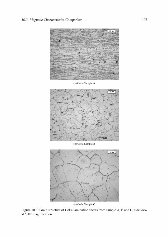
10.3. Magnetic Characteristics Comparison 107
(a) CoFe Sample A
(b) CoFe Sample B
(c) CoFe Sample C
Figure 10.3: Grain structure of CoFe lamination sheets from sample A, B and C, side viewat 500x magnification.
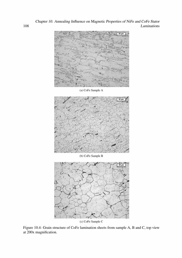
108Chapter 10. Annealing Influence on Magnetic Properties of NiFe and CoFe Stator
Laminations
(a) CoFe Sample A
(b) CoFe Sample B
(c) CoFe Sample C
Figure 10.4: Grain structure of CoFe lamination sheets from sample A, B and C, top viewat 200x magnification.
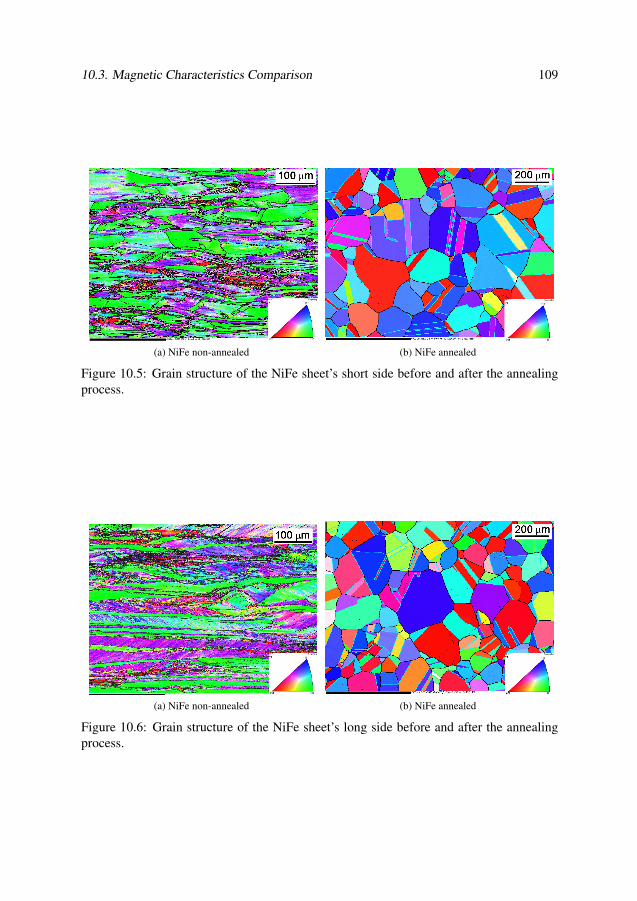
10.3. Magnetic Characteristics Comparison 109
(a) NiFe non-annealed (b) NiFe annealed
Figure 10.5: Grain structure of the NiFe sheet’s short side before and after the annealingprocess.
(a) NiFe non-annealed (b) NiFe annealed
Figure 10.6: Grain structure of the NiFe sheet’s long side before and after the annealingprocess.
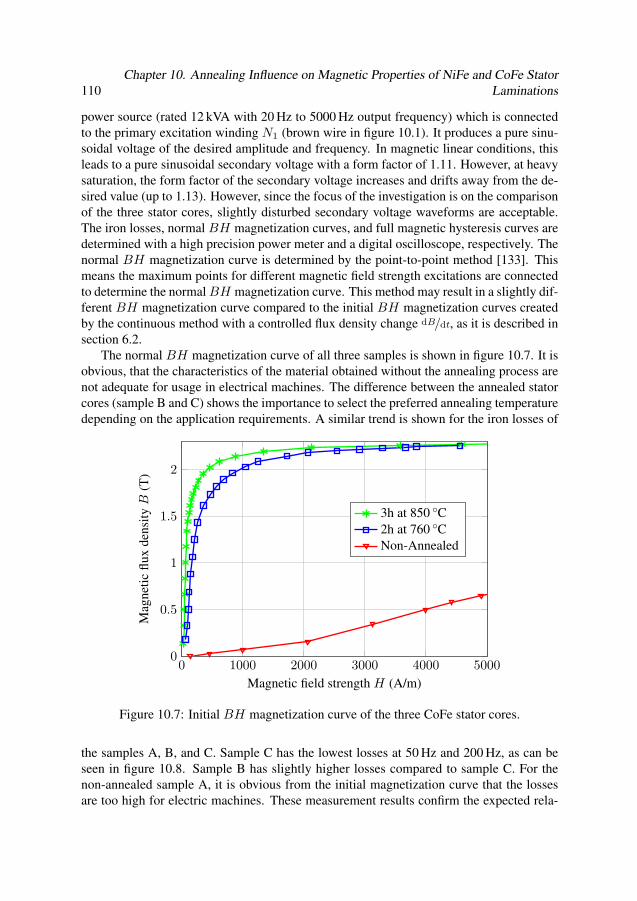
110Chapter 10. Annealing Influence on Magnetic Properties of NiFe and CoFe Stator
Laminations
power source (rated 12 kVA with 20 Hz to 5000 Hz output frequency) which is connectedto the primary excitation winding N1 (brown wire in figure 10.1). It produces a pure sinu-soidal voltage of the desired amplitude and frequency. In magnetic linear conditions, thisleads to a pure sinusoidal secondary voltage with a form factor of 1.11. However, at heavysaturation, the form factor of the secondary voltage increases and drifts away from the de-sired value (up to 1.13). However, since the focus of the investigation is on the comparisonof the three stator cores, slightly disturbed secondary voltage waveforms are acceptable.The iron losses, normal BH magnetization curves, and full magnetic hysteresis curves aredetermined with a high precision power meter and a digital oscilloscope, respectively. Thenormal BH magnetization curve is determined by the point-to-point method [133]. Thismeans the maximum points for different magnetic field strength excitations are connectedto determine the normal BH magnetization curve. This method may result in a slightly dif-ferent BH magnetization curve compared to the initial BH magnetization curves createdby the continuous method with a controlled flux density change dB/dt, as it is described insection 6.2.
The normal BH magnetization curve of all three samples is shown in figure 10.7. It isobvious, that the characteristics of the material obtained without the annealing process arenot adequate for usage in electrical machines. The difference between the annealed statorcores (sample B and C) shows the importance to select the preferred annealing temperaturedepending on the application requirements. A similar trend is shown for the iron losses of
0 1000 2000 3000 4000 50000
0.5
1
1.5
2
Magnetic field strength H (A/m)
Mag
neti
cfl
uxde
nsit
yB
(T)
3h at 850 C2h at 760 CNon-Annealed
Figure 10.7: Initial BH magnetization curve of the three CoFe stator cores.
the samples A, B, and C. Sample C has the lowest losses at 50 Hz and 200 Hz, as can beseen in figure 10.8. Sample B has slightly higher losses compared to sample C. For thenon-annealed sample A, it is obvious from the initial magnetization curve that the lossesare too high for electric machines. These measurement results confirm the expected rela-
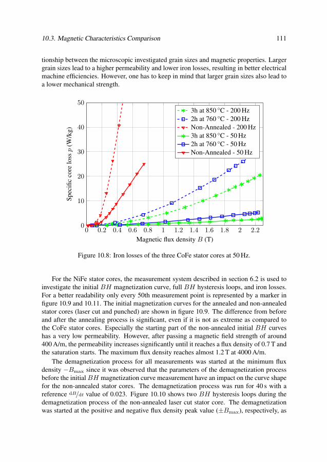
10.3. Magnetic Characteristics Comparison 111
tionship between the microscopic investigated grain sizes and magnetic properties. Largergrain sizes lead to a higher permeability and lower iron losses, resulting in better electricalmachine efficiencies. However, one has to keep in mind that larger grain sizes also lead toa lower mechanical strength.
0 0.2 0.4 0.6 0.8 1 1.2 1.4 1.6 1.8 2 2.20
10
20
30
40
50
Magnetic flux density B (T)
Spe
cifi
cco
relo
ssp
(W/k
g)
3h at 850 C - 200 Hz2h at 760 C - 200 HzNon-Annealed - 200 Hz3h at 850 C - 50 Hz2h at 760 C - 50 HzNon-Annealed - 50 Hz
Figure 10.8: Iron losses of the three CoFe stator cores at 50 Hz.
For the NiFe stator cores, the measurement system described in section 6.2 is used toinvestigate the initial BH magnetization curve, full BH hysteresis loops, and iron losses.For a better readability only every 50th measurement point is represented by a marker infigure 10.9 and 10.11. The initial magnetization curves for the annealed and non-annealedstator cores (laser cut and punched) are shown in figure 10.9. The difference from beforeand after the annealing process is significant, even if it is not as extreme as compared tothe CoFe stator cores. Especially the starting part of the non-annealed initial BH curveshas a very low permeability. However, after passing a magnetic field strength of around400 A/m, the permeability increases significantly until it reaches a flux density of 0.7 T andthe saturation starts. The maximum flux density reaches almost 1.2 T at 4000 A/m.
The demagnetization process for all measurements was started at the minimum fluxdensity −Bmax since it was observed that the parameters of the demagnetization processbefore the initial BH magnetization curve measurement have an impact on the curve shapefor the non-annealed stator cores. The demagnetization process was run for 40 s with areference dB/dt value of 0.023. Figure 10.10 shows two BH hysteresis loops during thedemagnetization process of the non-annealed laser cut stator core. The demagnetizationwas started at the positive and negative flux density peak value (±Bmax), respectively, as
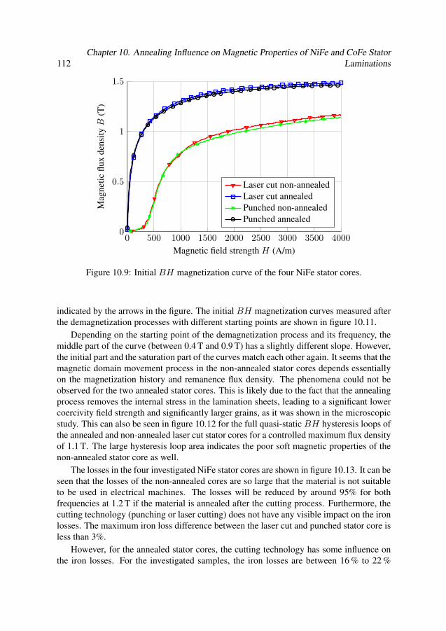
112Chapter 10. Annealing Influence on Magnetic Properties of NiFe and CoFe Stator
Laminations
0 500 1000 1500 2000 2500 3000 3500 40000
0.5
1
1.5
Magnetic field strength H (A/m)
Mag
neti
cfl
uxde
nsit
yB
(T)
Laser cut non-annealedLaser cut annealedPunched non-annealedPunched annealed
Figure 10.9: Initial BH magnetization curve of the four NiFe stator cores.
indicated by the arrows in the figure. The initial BH magnetization curves measured afterthe demagnetization processes with different starting points are shown in figure 10.11.
Depending on the starting point of the demagnetization process and its frequency, themiddle part of the curve (between 0.4 T and 0.9 T) has a slightly different slope. However,the initial part and the saturation part of the curves match each other again. It seems that themagnetic domain movement process in the non-annealed stator cores depends essentiallyon the magnetization history and remanence flux density. The phenomena could not beobserved for the two annealed stator cores. This is likely due to the fact that the annealingprocess removes the internal stress in the lamination sheets, leading to a significant lowercoercivity field strength and significantly larger grains, as it was shown in the microscopicstudy. This can also be seen in figure 10.12 for the full quasi-static BH hysteresis loops ofthe annealed and non-annealed laser cut stator cores for a controlled maximum flux densityof 1.1 T. The large hysteresis loop area indicates the poor soft magnetic properties of thenon-annealed stator core as well.
The losses in the four investigated NiFe stator cores are shown in figure 10.13. It can beseen that the losses of the non-annealed cores are so large that the material is not suitableto be used in electrical machines. The losses will be reduced by around 95% for bothfrequencies at 1.2 T if the material is annealed after the cutting process. Furthermore, thecutting technology (punching or laser cutting) does not have any visible impact on the ironlosses. The maximum iron loss difference between the laser cut and punched stator core isless than 3%.
However, for the annealed stator cores, the cutting technology has some influence onthe iron losses. For the investigated samples, the iron losses are between 16 % to 22 %

10.3. Magnetic Characteristics Comparison 113
−3000 −2000 −1000 0 1000 2000 3000
−1
−0.5
0
0.5
1
+Bmax
−Bmax
Magnetic field strength H (A/m)
Mag
neti
cfl
uxde
nsit
yB
(T)
+Bmax demagnetization−Bmax demagnetization
Figure 10.10: Demagnetization curves of the non-annealed laser cut NiFe stator core withdifferent demagnetization starting points.
0 500 1000 1500 2000 2500 3000 3500 40000
0.5
1
1.5
Magnetic field strength H (A/m)
Mag
neti
cfl
uxde
nsit
yB
(T)
+Bmax demagnetization−Bmax demagnetization
Figure 10.11: Initial BH magnetization curves of the non-annealed laser cut NiFe statorcore after different demagnetization starting points as shown in figure 10.10.
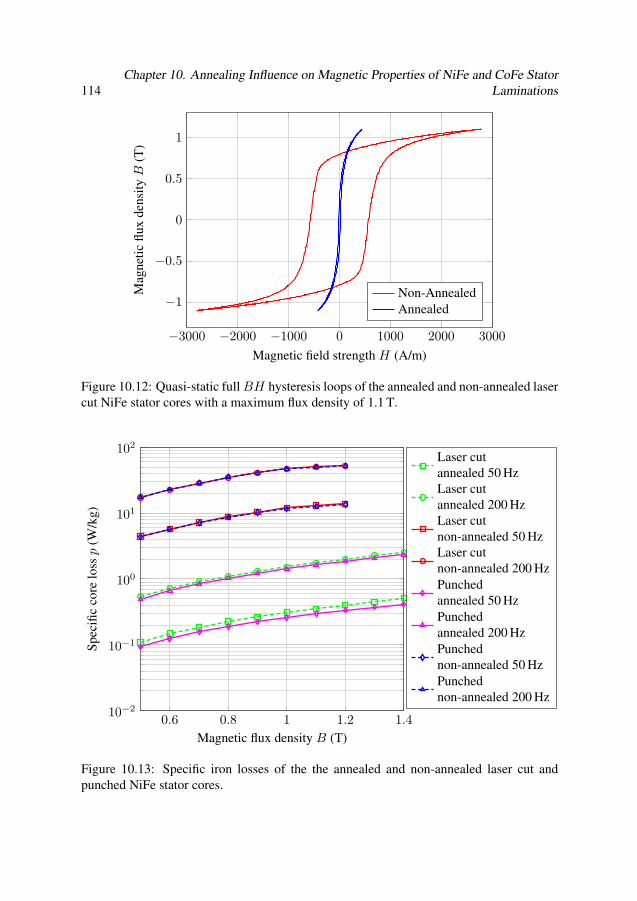
114Chapter 10. Annealing Influence on Magnetic Properties of NiFe and CoFe Stator
Laminations
−3000 −2000 −1000 0 1000 2000 3000
−1
−0.5
0
0.5
1
Magnetic field strength H (A/m)
Mag
neti
cfl
uxde
nsit
yB
(T)
Non-AnnealedAnnealed
Figure 10.12: Quasi-static full BH hysteresis loops of the annealed and non-annealed lasercut NiFe stator cores with a maximum flux density of 1.1 T.
0.6 0.8 1 1.2 1.410−2
10−1
100
101
102
Magnetic flux density B (T)
Spe
cifi
cco
relo
ssp
(W/k
g)
Laser cutannealed 50 HzLaser cutannealed 200 HzLaser cutnon-annealed 50 HzLaser cutnon-annealed 200 HzPunchedannealed 50 HzPunchedannealed 200 HzPunchednon-annealed 50 HzPunchednon-annealed 200 Hz
Figure 10.13: Specific iron losses of the the annealed and non-annealed laser cut andpunched NiFe stator cores.
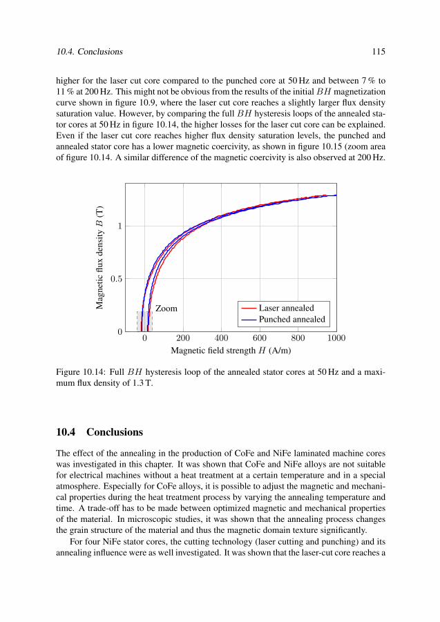
10.4. Conclusions 115
higher for the laser cut core compared to the punched core at 50 Hz and between 7 % to11 % at 200 Hz. This might not be obvious from the results of the initial BH magnetizationcurve shown in figure 10.9, where the laser cut core reaches a slightly larger flux densitysaturation value. However, by comparing the full BH hysteresis loops of the annealed sta-tor cores at 50 Hz in figure 10.14, the higher losses for the laser cut core can be explained.Even if the laser cut core reaches higher flux density saturation levels, the punched andannealed stator core has a lower magnetic coercivity, as shown in figure 10.15 (zoom areaof figure 10.14. A similar difference of the magnetic coercivity is also observed at 200 Hz.
0 200 400 600 800 10000
0.5
1
Zoom
Magnetic field strength H (A/m)
Mag
neti
cfl
uxde
nsit
yB
(T)
Laser annealedPunched annealed
Figure 10.14: Full BH hysteresis loop of the annealed stator cores at 50 Hz and a maxi-mum flux density of 1.3 T.
10.4 Conclusions
The effect of the annealing in the production of CoFe and NiFe laminated machine coreswas investigated in this chapter. It was shown that CoFe and NiFe alloys are not suitablefor electrical machines without a heat treatment at a certain temperature and in a specialatmosphere. Especially for CoFe alloys, it is possible to adjust the magnetic and mechani-cal properties during the heat treatment process by varying the annealing temperature andtime. A trade-off has to be made between optimized magnetic and mechanical propertiesof the material. In microscopic studies, it was shown that the annealing process changesthe grain structure of the material and thus the magnetic domain texture significantly.
For four NiFe stator cores, the cutting technology (laser cutting and punching) and itsannealing influence were as well investigated. It was shown that the laser-cut core reaches a
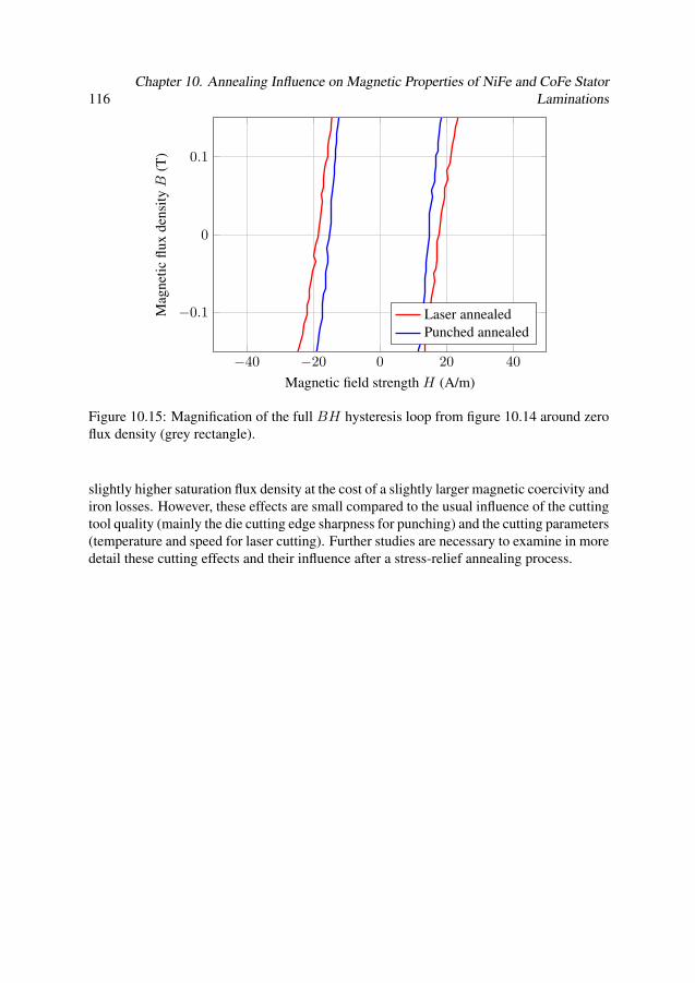
116Chapter 10. Annealing Influence on Magnetic Properties of NiFe and CoFe Stator
Laminations
−40 −20 0 20 40
−0.1
0
0.1
Magnetic field strength H (A/m)
Mag
neti
cfl
uxde
nsit
yB
(T)
Laser annealedPunched annealed
Figure 10.15: Magnification of the full BH hysteresis loop from figure 10.14 around zeroflux density (grey rectangle).
slightly higher saturation flux density at the cost of a slightly larger magnetic coercivity andiron losses. However, these effects are small compared to the usual influence of the cuttingtool quality (mainly the die cutting edge sharpness for punching) and the cutting parameters(temperature and speed for laser cutting). Further studies are necessary to examine in moredetail these cutting effects and their influence after a stress-relief annealing process.
Chapter 11
Thermal Measurements to Investigate
Iron Losses
In this chapter, methods based on thermal models for experimental loss identifications are
presented. Experiments, thermal network modelling, and finite element method (FEM)
simulations are carried out on an outer-rotor permanent magnet synchronous machine
(PMSM) for household applications. Several methods for identifying and separating losses
in different parts of the machine are investigated. Thermal lumped parameter (LP) models
and 3D FEM simulations are used to determine temperature and flux density distributions,
as well as iron losses in the magnetic steel parts of the machine. Afterwards, thermal
measurements are conducted to derive losses and study the loss distribution in the machine
experimentally by transient thermal measurements (inverse thermal modelling). Finally,
the measurements are compared to the FEM simulations and evaluated.
11.1 Thermal Methods to Determine Losses
A physical measurable quantity related to losses is the temperature. In most applicationstemperature distributions are determined from generated losses in the devices. However,temperature distributions and changes can also be used contrary to determine losses [134],[135]. The simplest method for thermal modelling of electrical machines is the lumpedparameter (LP) model. The dynamic LP model consists of thermal resistances and capaci-tances for describing the heat flow characteristics and thermal distribution in the machine.Losses are modelled as thermal heat sources. Figure 11.1 gives an example of the LPmodel of the investigated outer-rotor PMSM in this chapter.
A thermal loss investigation on a 5.5 kW induction motor equipped with 100 ther-mal sensors in the stator and squirrel cage rotor is presented in [136]. In this study, thelosses are determined by inverting and over-determining the matrix of the thermal lumped-parameter machine model at steady-state. A transient thermal loss investigation for de-termining losses from temperature changes by applying an inverse thermal model (ITM)method is presented in [137]. The method is applied on a large water-wheel synchronous
117
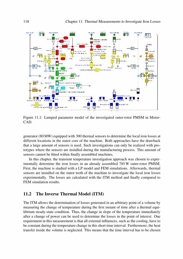
118 Chapter 11. Thermal Measurements to Investigate Iron Losses
Figure 11.1: Lumped parameter model of the investigated outer-rotor PMSM in Motor-CAD.
generator (80 MW) equipped with 300 thermal sensors to determine the local iron losses atdifferent locations in the stator core of the machine. Both approaches have the drawbackthat a large amount of sensors is used. Such investigations can only be realized with pro-totypes where the sensors are installed during the manufacturing process. This amount ofsensors cannot be fitted within finally assembled machines.
In this chapter, the transient temperature investigation approach was chosen to exper-imentally determine the iron losses in an already assembled 785 W outer-rotor PMSM.First, the machine is studied with a LP model and FEM simulations. Afterwards, thermalsensors are installed on the stator teeth of the machine to investigate the local iron lossesexperimentally. The losses are calculated with the ITM method and finally compared toFEM simulation results.
11.2 The Inverse Thermal Model (ITM)
The ITM allows the determination of losses generated in an arbitrary point of a volume bymeasuring the change of temperature during the first instant of time after a thermal equi-librium steady-state condition. Thus, the change in slope of the temperature immediatelyafter a change of power can be used to determine the losses in the point of interest. Onerequirement in this measurement is that all external influences, such as the cooling, have tobe constant during the temperature change in this short time interval. Furthermore, the heattransfer inside the volume is neglected. This means that the time interval has to be chosen
11.2. The Inverse Thermal Model (ITM) 119
short enough, so that no heat transfer occurs inside the volume during the measurementtime. The heat capacity of the investigated volume must also be available and the influencedue to the heat capacity of the thermal mounted sensor negligible or accounted for.
Assuming constant material properties (e.g. isotropic material and the thermal conduc-tivity and specific heat capacitance are not depending on the temperature), the general heatdiffusion equation (often called heat equation) can be expressed as [138],[139]
∂ϑ
∂ t= a ∇2ϑ +
pgen
cth γ, (11.1)
with the thermal diffusivity
a =σth
cth γ. (11.2)
In (11.1) and (11.2), cth is the specific thermal capacity in J/(kg K), γ the material densityin kg/m3, σth the thermal conductivity in W/(K m), pgen the specific power density inW/m3, and ϑ the temperature in K.
At steady state, (11.1) states that the power generation or absorption inside an inves-tigated volume is equal to its local temperature distribution. It is used as the initial pointof the ITM. The measurement is started from a steady-state condition with constant dis-tributed temperature in a volume which is a small part of the investigated device. Then, thepower generation inside the investigated volume is changed instantly and (11.1) evolves to(11.3)
(
∂ϑ
∂ t
)
t→0+
= a∇2ϑ +pgen
cth γ. (11.3)
It is now assumed that the heat transfer inside the investigated volume is negligible duringthe first instant after the power change. This means that a ∇2 ϑ ≪
pgen
cth γis fulfilled. In
this case, the diffusion term on the right hand side of (11.3) can be neglected and (11.3)simplifies to
(
∂ϑ
∂ t
)
t→0+
=pgen
cth γ. (11.4)
Reordering (11.4) yields
pgen = cthγ
(
∂ϑ
∂ t
)
t→0+
, (11.5)
which is referred to as the inverse thermal model (ITM) in the following.The difficulty of the ITM consists in the estimation of the time interval which needs
to be investigated to fulfil the condition σth
cth γ∇2 ϑ ≪
pgen
cth γ. The thermal time constant
cth γσth
on the left hand side of this condition is only simple to determine if the volume of theinvestigated device is small and has clear determined borders. But this is often not the case

120 Chapter 11. Thermal Measurements to Investigate Iron Losses
for complex machine geometries. Furthermore, the term ∇2 ϑ of the condition is a directfunction of the temperature change and makes a rough estimation relatively difficult.
In summary, it is not possible to define a general time period for the measured temper-ature slope to investigate. In [137], a time period of less than 30 seconds is used to achievesatisfactory results for a 80 MW waterwheel alternator, 20 seconds are used for a 4 kWTEFC induction motor in [140]. In the study of the 5.5 kW induction machine no informa-tion about the used time periods and applied temperature slopes in the loss calculations isgiven [136], [141].
11.3 Thermal Analysis of an Outer Rotor Permanent Magnet
Machine
The investigated outer-rotor PMSM shown in figure 11.2 has a concentrated double-layerwinding with 28 poles and 24 slots. Ferrite permanent magnets are mounted on the insidesurface of the outer rotor. The stator core is built from M800-50A SiFe lamination sheetsand each tooth is wound with 181 turns. The rotor core is made of solid steel. Moretechnical data of the motor is reported in table 11.1.
Figure 11.2: Stator and rotor with axial cooling ducts of the investigated outer-rotorPMSM.
The machine is modelled with the Motor-CAD1 software package to investigate theheat distribution inside the machine and the expected initial temperature changes andsteady state conditions in more detail. The Motor-CAD model of the machine is shownin figure 11.3. The material parameters used in the Motor-CAD model are listed in ta-ble 11.2. In Motor-CAD, the temperature is an output variable depending on the losses inthe machine. Therefore, the losses obtained by experiments conducted by Dr. FlorenceMeier are used for initial simulations [144]. Furthermore, the following assumptions forthe machine model are made:
1Motor-CAD is a thermal simulation software for electrical machines from Motor Design Ltd, UK.

11.3. Thermal Analysis of an Outer Rotor Permanent Magnet Machine 121
Table 11.1: Technical data of the investigated outer-rotor PMSM.
Number of poles: 28
Number of slots: 24Number of turns per tooth coil: 181
Slot fill factor: 0.4Rated torque: 30 Nm
Rated speed: 200 rpm
Maximum speed: 1200 rpm
Maximum power: 785 W
Rated current (RMS): 3.4 A
Resistance (line-to-line): 5.3 Ω
Magnet remanent flux density Br at 25 C: 0.41 T
Measured d-axis inductance Ld: 0.96 mH
Rotor outer diameter [mm]: 404
Stator outer diameter [mm]: 374
Airgap length [mm]: 1
Axial length stator [mm]: 20
Active axial length rotor [mm]: 25
Figure 11.3: The machine model in Motor-CAD, front and axial view.
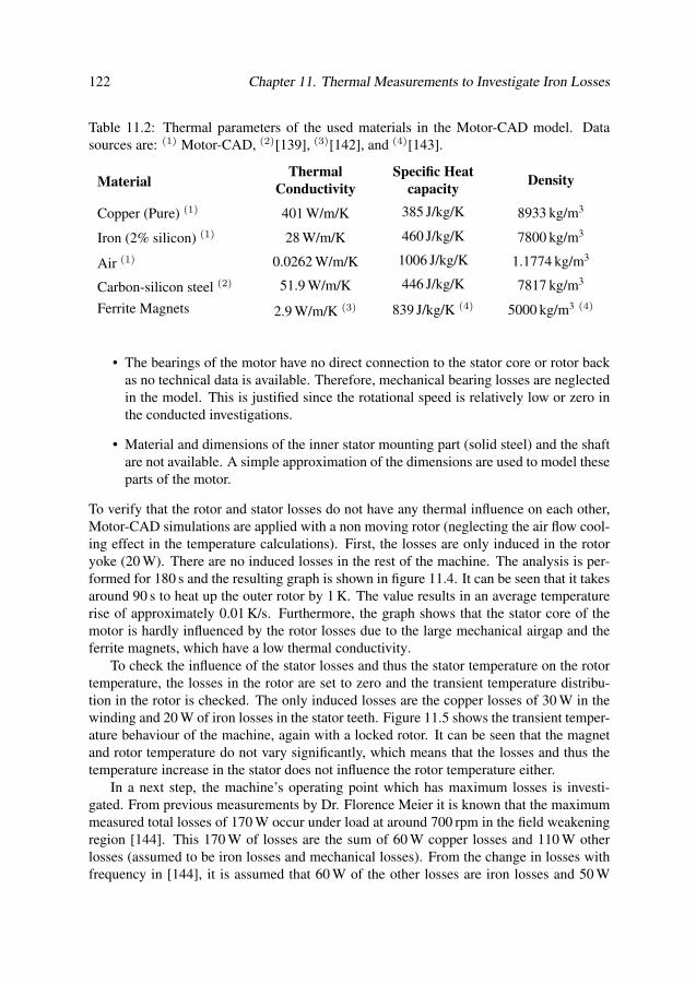
122 Chapter 11. Thermal Measurements to Investigate Iron Losses
Table 11.2: Thermal parameters of the used materials in the Motor-CAD model. Datasources are: (1) Motor-CAD, (2)[139], (3)[142], and (4)[143].
MaterialThermal
Conductivity
Specific Heat
capacityDensity
Copper (Pure) (1) 401 W/m/K 385 J/kg/K 8933 kg/m3
Iron (2% silicon) (1) 28 W/m/K 460 J/kg/K 7800 kg/m3
Air (1) 0.0262 W/m/K 1006 J/kg/K 1.1774 kg/m3
Carbon-silicon steel (2) 51.9 W/m/K 446 J/kg/K 7817 kg/m3
Ferrite Magnets 2.9 W/m/K (3) 839 J/kg/K (4) 5000 kg/m3 (4)
• The bearings of the motor have no direct connection to the stator core or rotor backas no technical data is available. Therefore, mechanical bearing losses are neglectedin the model. This is justified since the rotational speed is relatively low or zero inthe conducted investigations.
• Material and dimensions of the inner stator mounting part (solid steel) and the shaftare not available. A simple approximation of the dimensions are used to model theseparts of the motor.
To verify that the rotor and stator losses do not have any thermal influence on each other,Motor-CAD simulations are applied with a non moving rotor (neglecting the air flow cool-ing effect in the temperature calculations). First, the losses are only induced in the rotoryoke (20 W). There are no induced losses in the rest of the machine. The analysis is per-formed for 180 s and the resulting graph is shown in figure 11.4. It can be seen that it takesaround 90 s to heat up the outer rotor by 1 K. The value results in an average temperaturerise of approximately 0.01 K/s. Furthermore, the graph shows that the stator core of themotor is hardly influenced by the rotor losses due to the large mechanical airgap and theferrite magnets, which have a low thermal conductivity.
To check the influence of the stator losses and thus the stator temperature on the rotortemperature, the losses in the rotor are set to zero and the transient temperature distribu-tion in the rotor is checked. The only induced losses are the copper losses of 30 W in thewinding and 20 W of iron losses in the stator teeth. Figure 11.5 shows the transient temper-ature behaviour of the machine, again with a locked rotor. It can be seen that the magnetand rotor temperature do not vary significantly, which means that the losses and thus thetemperature increase in the stator does not influence the rotor temperature either.
In a next step, the machine’s operating point which has maximum losses is investi-gated. From previous measurements by Dr. Florence Meier it is known that the maximummeasured total losses of 170 W occur under load at around 700 rpm in the field weakeningregion [144]. This 170 W of losses are the sum of 60 W copper losses and 110 W otherlosses (assumed to be iron losses and mechanical losses). From the change in losses withfrequency in [144], it is assumed that 60 W of the other losses are iron losses and 50 W
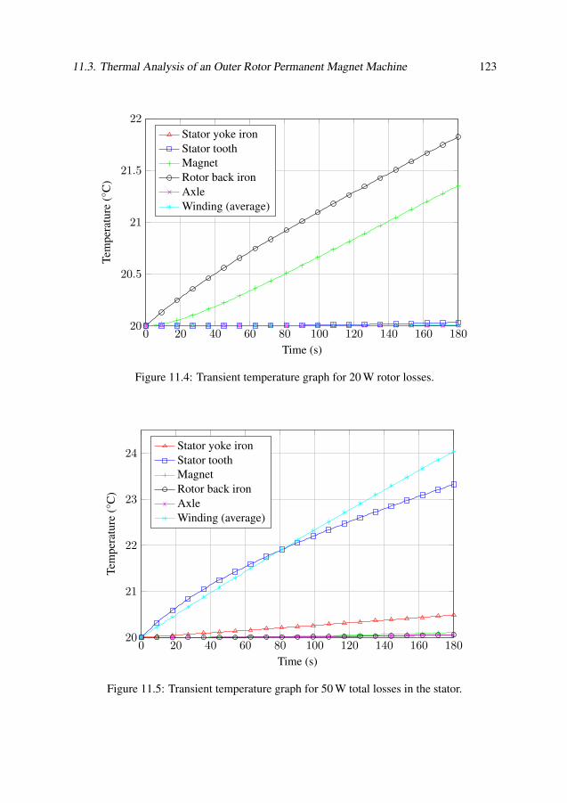
11.3. Thermal Analysis of an Outer Rotor Permanent Magnet Machine 123
0 20 40 60 80 100 120 140 160 18020
20.5
21
21.5
22
Time (s)
Tem
pera
ture
(C
)
Stator yoke ironStator toothMagnetRotor back ironAxleWinding (average)
Figure 11.4: Transient temperature graph for 20 W rotor losses.
0 20 40 60 80 100 120 140 160 18020
21
22
23
24
Time (s)
Tem
pera
ture
(C
)
Stator yoke ironStator toothMagnetRotor back ironAxleWinding (average)
Figure 11.5: Transient temperature graph for 50 W total losses in the stator.
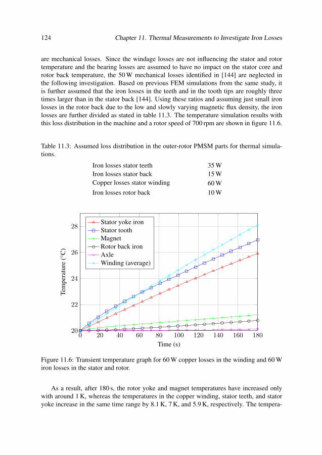
124 Chapter 11. Thermal Measurements to Investigate Iron Losses
are mechanical losses. Since the windage losses are not influencing the stator and rotortemperature and the bearing losses are assumed to have no impact on the stator core androtor back temperature, the 50 W mechanical losses identified in [144] are neglected inthe following investigation. Based on previous FEM simulations from the same study, itis further assumed that the iron losses in the teeth and in the tooth tips are roughly threetimes larger than in the stator back [144]. Using these ratios and assuming just small ironlosses in the rotor back due to the low and slowly varying magnetic flux density, the ironlosses are further divided as stated in table 11.3. The temperature simulation results withthis loss distribution in the machine and a rotor speed of 700 rpm are shown in figure 11.6.
Table 11.3: Assumed loss distribution in the outer-rotor PMSM parts for thermal simula-tions.
Iron losses stator teeth 35 WIron losses stator back 15 WCopper losses stator winding 60 W
Iron losses rotor back 10 W
0 20 40 60 80 100 120 140 160 18020
22
24
26
28
Time (s)
Tem
pera
ture
(C
)
Stator yoke ironStator toothMagnetRotor back ironAxleWinding (average)
Figure 11.6: Transient temperature graph for 60 W copper losses in the winding and 60 Wiron losses in the stator and rotor.
As a result, after 180 s, the rotor yoke and magnet temperatures have increased onlywith around 1 K, whereas the temperatures in the copper winding, stator teeth, and statoryoke increase in the same time range by 8.1 K, 7 K, and 5.9 K, respectively. The tempera-
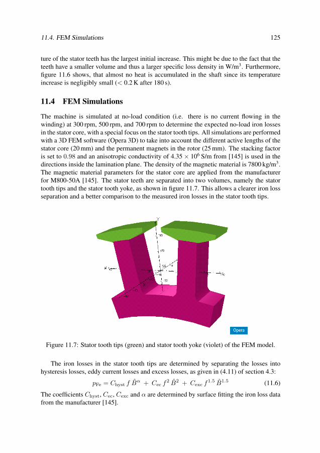
11.4. FEM Simulations 125
ture of the stator teeth has the largest initial increase. This might be due to the fact that theteeth have a smaller volume and thus a larger specific loss density in W/m3. Furthermore,figure 11.6 shows, that almost no heat is accumulated in the shaft since its temperatureincrease is negligibly small (< 0.2 K after 180 s).
11.4 FEM Simulations
The machine is simulated at no-load condition (i.e. there is no current flowing in thewinding) at 300 rpm, 500 rpm, and 700 rpm to determine the expected no-load iron lossesin the stator core, with a special focus on the stator tooth tips. All simulations are performedwith a 3D FEM software (Opera 3D) to take into account the different active lengths of thestator core (20 mm) and the permanent magnets in the rotor (25 mm). The stacking factoris set to 0.98 and an anisotropic conductivity of 4.35 × 10⁶ S/m from [145] is used in thedirections inside the lamination plane. The density of the magnetic material is 7800 kg/m3.The magnetic material parameters for the stator core are applied from the manufacturerfor M800-50A [145]. The stator teeth are separated into two volumes, namely the statortooth tips and the stator tooth yoke, as shown in figure 11.7. This allows a clearer iron lossseparation and a better comparison to the measured iron losses in the stator tooth tips.
Figure 11.7: Stator tooth tips (green) and stator tooth yoke (violet) of the FEM model.
The iron losses in the stator tooth tips are determined by separating the losses intohysteresis losses, eddy current losses and excess losses, as given in (4.11) of section 4.3:
pFe = Chyst f Bα + Cec f2 B2 + Cexc f1.5 B1.5 (11.6)
The coefficients Chyst, Cec, Cexc and α are determined by surface fitting the iron loss datafrom the manufacturer [145].
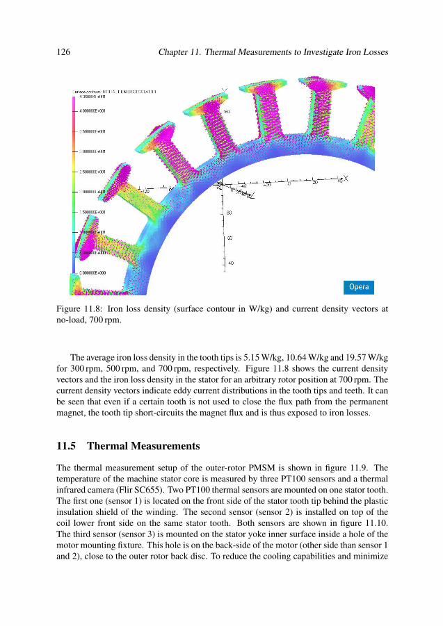
126 Chapter 11. Thermal Measurements to Investigate Iron Losses
Figure 11.8: Iron loss density (surface contour in W/kg) and current density vectors atno-load, 700 rpm.
The average iron loss density in the tooth tips is 5.15 W/kg, 10.64 W/kg and 19.57 W/kgfor 300 rpm, 500 rpm, and 700 rpm, respectively. Figure 11.8 shows the current densityvectors and the iron loss density in the stator for an arbitrary rotor position at 700 rpm. Thecurrent density vectors indicate eddy current distributions in the tooth tips and teeth. It canbe seen that even if a certain tooth is not used to close the flux path from the permanentmagnet, the tooth tip short-circuits the magnet flux and is thus exposed to iron losses.
11.5 Thermal Measurements
The thermal measurement setup of the outer-rotor PMSM is shown in figure 11.9. Thetemperature of the machine stator core is measured by three PT100 sensors and a thermalinfrared camera (Flir SC655). Two PT100 thermal sensors are mounted on one stator tooth.The first one (sensor 1) is located on the front side of the stator tooth tip behind the plasticinsulation shield of the winding. The second sensor (sensor 2) is installed on top of thecoil lower front side on the same stator tooth. Both sensors are shown in figure 11.10.The third sensor (sensor 3) is mounted on the stator yoke inner surface inside a hole of themotor mounting fixture. This hole is on the back-side of the motor (other side than sensor 1and 2), close to the outer rotor back disc. To reduce the cooling capabilities and minimize

11.5. Thermal Measurements 127
Figure 11.9: Thermal measurement setup of the investigated outer-rotor PMSM.
the turbulent air flow in the machine, the axial cooling ducts on the back side of the rotordisc, visible on the right hand side in figure 11.2, are covered with transparent tape.
For the no-load tests, the investigated outer-rotor PMSM with open terminals is drivenby a synchronous machine at constant speed, so that there is no current flowing in thewindings. It is assumed that all measured losses and all of the corresponding temperatureincreases in the stator core are caused by iron losses (friction and windage losses can beneglected since they do not heat up the stator core during the investigation time). The testsare performed at 300 rpm, 500 rpm, and 700 rpm at constant room temperature (22 C).The temperature sensors are sampled every third second and the thermal infrared camerarecords the temperature at a sampling rate of 10 Hz. Figure 11.11 shows a thermal pic-ture of the stator teeth and coils during no-load test with 700 rpm after several minutes ofoperation.
The measurement results of the PT100 temperature sensors 1 and 3 are shown in fig-ure 11.12. Sensor 1 (mounted on the stator tooth tip front side) has the largest temperatureraise due to iron losses in the tooth tips induced from the flux of the permanent magnets.With increasing speed of the rotor, the frequency of the flux in the stator core increasesand thus the iron losses as well. Sensor 3 (mounted on the stator yoke back side) has asmaller temperature increase due to lower iron losses in the stator yoke and a turbulent airflow around the sensor created by the rotations of the rotor. This air flow might also be thecause for the delayed temperature rise compared to sensor 1. The temperature increase ofthe winding surface (sensor 2) is marginal in the no-load case and just caused by the heattransfer from the stator teeth and tooth tips through the copper coil winding. Therefore, it

128 Chapter 11. Thermal Measurements to Investigate Iron Losses
Figure 11.10: PT100 temperature sensors mounted on the front side of the stator tooth tipand on the winding coil.
Figure 11.11: Thermal image of the stator coils and mounted PT100 sensors at a no-loadtest with 700 rpm.
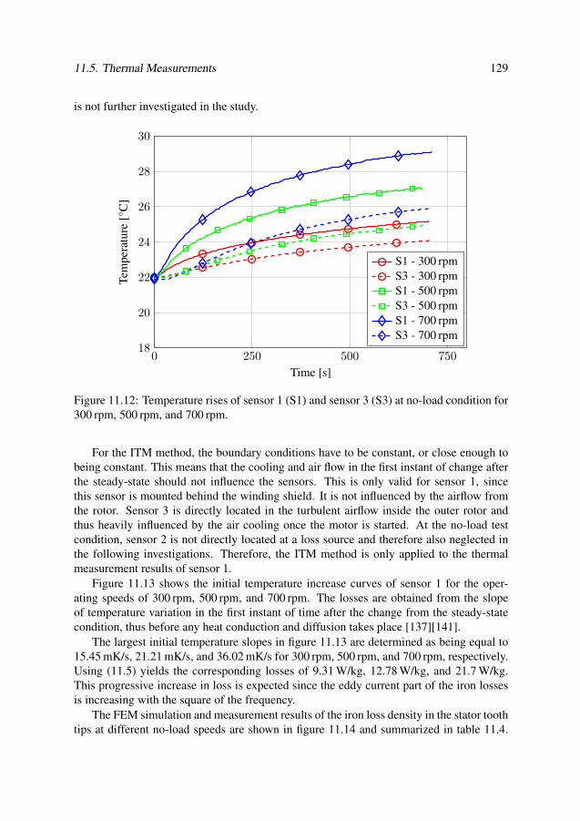
11.5. Thermal Measurements 129
is not further investigated in the study.
0 250 500 75018
20
22
24
26
28
30
Time [s]
Tem
pera
ture
[C
]
S1 - 300 rpmS3 - 300 rpmS1 - 500 rpmS3 - 500 rpmS1 - 700 rpmS3 - 700 rpm
Figure 11.12: Temperature rises of sensor 1 (S1) and sensor 3 (S3) at no-load condition for300 rpm, 500 rpm, and 700 rpm.
For the ITM method, the boundary conditions have to be constant, or close enough tobeing constant. This means that the cooling and air flow in the first instant of change afterthe steady-state should not influence the sensors. This is only valid for sensor 1, sincethis sensor is mounted behind the winding shield. It is not influenced by the airflow fromthe rotor. Sensor 3 is directly located in the turbulent airflow inside the outer rotor andthus heavily influenced by the air cooling once the motor is started. At the no-load testcondition, sensor 2 is not directly located at a loss source and therefore also neglected inthe following investigations. Therefore, the ITM method is only applied to the thermalmeasurement results of sensor 1.
Figure 11.13 shows the initial temperature increase curves of sensor 1 for the oper-ating speeds of 300 rpm, 500 rpm, and 700 rpm. The losses are obtained from the slopeof temperature variation in the first instant of time after the change from the steady-statecondition, thus before any heat conduction and diffusion takes place [137][141].
The largest initial temperature slopes in figure 11.13 are determined as being equal to15.45 mK/s, 21.21 mK/s, and 36.02 mK/s for 300 rpm, 500 rpm, and 700 rpm, respectively.Using (11.5) yields the corresponding losses of 9.31 W/kg, 12.78 W/kg, and 21.7 W/kg.This progressive increase in loss is expected since the eddy current part of the iron lossesis increasing with the square of the frequency.
The FEM simulation and measurement results of the iron loss density in the stator toothtips at different no-load speeds are shown in figure 11.14 and summarized in table 11.4.
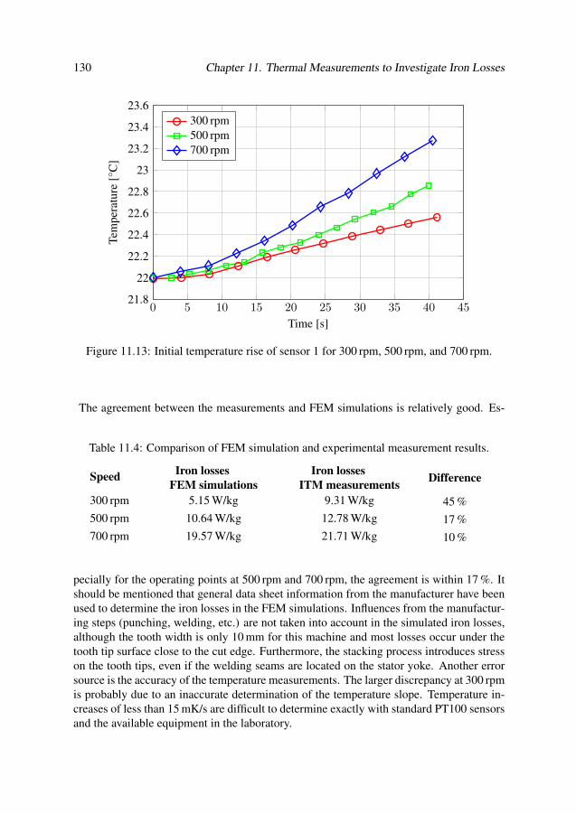
130 Chapter 11. Thermal Measurements to Investigate Iron Losses
0 5 10 15 20 25 30 35 40 4521.8
22
22.2
22.4
22.6
22.8
23
23.2
23.4
23.6
Time [s]
Tem
pera
ture
[C
]300 rpm500 rpm700 rpm
Figure 11.13: Initial temperature rise of sensor 1 for 300 rpm, 500 rpm, and 700 rpm.
The agreement between the measurements and FEM simulations is relatively good. Es-
Table 11.4: Comparison of FEM simulation and experimental measurement results.
SpeedIron losses
FEM simulations
Iron losses
ITM measurementsDifference
300 rpm 5.15 W/kg 9.31 W/kg 45 %
500 rpm 10.64 W/kg 12.78 W/kg 17 %
700 rpm 19.57 W/kg 21.71 W/kg 10 %
pecially for the operating points at 500 rpm and 700 rpm, the agreement is within 17 %. Itshould be mentioned that general data sheet information from the manufacturer have beenused to determine the iron losses in the FEM simulations. Influences from the manufactur-ing steps (punching, welding, etc.) are not taken into account in the simulated iron losses,although the tooth width is only 10 mm for this machine and most losses occur under thetooth tip surface close to the cut edge. Furthermore, the stacking process introduces stresson the tooth tips, even if the welding seams are located on the stator yoke. Another errorsource is the accuracy of the temperature measurements. The larger discrepancy at 300 rpmis probably due to an inaccurate determination of the temperature slope. Temperature in-creases of less than 15 mK/s are difficult to determine exactly with standard PT100 sensorsand the available equipment in the laboratory.
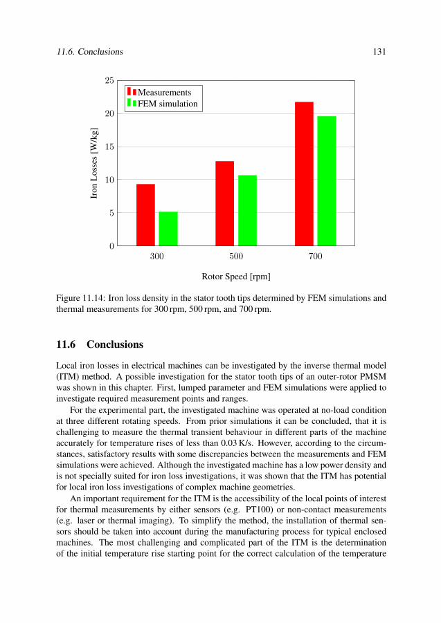
11.6. Conclusions 131
300 500 7000
5
10
15
20
25
300 500 7000
5
10
15
20
25
Rotor Speed [rpm]
Iron
Los
ses
[W/k
g]MeasurementsFEM simulation
Figure 11.14: Iron loss density in the stator tooth tips determined by FEM simulations andthermal measurements for 300 rpm, 500 rpm, and 700 rpm.
11.6 Conclusions
Local iron losses in electrical machines can be investigated by the inverse thermal model(ITM) method. A possible investigation for the stator tooth tips of an outer-rotor PMSMwas shown in this chapter. First, lumped parameter and FEM simulations were applied toinvestigate required measurement points and ranges.
For the experimental part, the investigated machine was operated at no-load conditionat three different rotating speeds. From prior simulations it can be concluded, that it ischallenging to measure the thermal transient behaviour in different parts of the machineaccurately for temperature rises of less than 0.03 K/s. However, according to the circum-stances, satisfactory results with some discrepancies between the measurements and FEMsimulations were achieved. Although the investigated machine has a low power density andis not specially suited for iron loss investigations, it was shown that the ITM has potentialfor local iron loss investigations of complex machine geometries.
An important requirement for the ITM is the accessibility of the local points of interestfor thermal measurements by either sensors (e.g. PT100) or non-contact measurements(e.g. laser or thermal imaging). To simplify the method, the installation of thermal sen-sors should be taken into account during the manufacturing process for typical enclosedmachines. The most challenging and complicated part of the ITM is the determinationof the initial temperature rise starting point for the correct calculation of the temperature

132 Chapter 11. Thermal Measurements to Investigate Iron Losses
slope and thus the associated losses. Depending on the specific local losses, temperatureslopes in the range of several mK/s need to be determined accurately in order to achievesatisfactory results.
Chapter 12
Conclusions and Future Work
This chapter summarizes the work previously described in this thesis. Ideas and guidelines
for future work are presented, including a personal evaluation of priority.
12.1 Conclusions
Electrical machines play a fundamental role in the global electrical energy saving plans ofthe future. Various research activities are conducted to increase the efficiency of electricalmachines and to reduce the energy consumption. The magnetic materials and iron lossesin electrical machines play a key role in these efforts and have been the main focus of thisstudy.
Depending on the application, the electrical machine designer can choose from a wideselection of magnetic material alloys. Each material differs in its magnetic and mechani-cal properties and has a specific behaviour regarding the influences of the manufacturingprocess. To simplify the selection process with regard to the magnetic properties and ironlosses of the material, the author has suggested a graphical tool representing the iron lossesin the material over the squared flux density (PB2 factor), as it is described in chapter 5.With this tool, it is possible to compare the initial BH magnetization curves and the spe-cific iron losses for arbitrary magnetic materials graphically and at the same time. How-ever, several influencing factors, like the deterioration during the machine manufacturingprocess, machine manufacturing tolerances, and stress in the laminations, are not consid-ered in the material selection tool. Therefore, the method is to be seen as a starting pointfor the material selection in the machine design process.
Electrical machines have been around for more than 150 years and the first iron lossmodel was proposed around 130 years ago. However, researchers and electrical machinedesigners still struggle with the accuracy and influencing factors in today used iron lossmodels. The material influencing effects are often so complicated that it is very chal-lenging or even impossible to take them into account in general analytical or FEM-basedmachine models. The literature study of different iron loss models in chapter 4 revealedthat the challenge to find the correct model input parameters is one of the main reasons
133

134 Chapter 12. Conclusions and Future Work
for the discrepancies between the simulation and experimental results. The other reasonsfor inaccurate results of the iron loss models are the complex flux density waveforms inmodern electrical machine stator cores and the sophisticated machine geometries.
Typical Epstein frame measurements published in the manufacturers’ data-sheets donot take typical electrical machine geometries and, thus, also rotating losses into account.Furthermore, the degradation of the material due to the cutting/punching and welding pro-cess often changes the material properties significantly, leading to larger iron losses. Espe-cially for machine designs having small geometries (i.e. thin tooth and yoke widths due tohigh slot and pole numbers or small machines in general) it has been shown that the ironloss deviations between the manufacturers’ Epstein frame results and the final assembledstator core measurements can deviate by more than 50 %. The iron loss calculation in finiteelement method (FEM) simulation software is generally done as a post-processing step.The most common method in commercial FEM software is still the iron loss separationmodel (see section 4.3). However, this model assumes usually sinusoidal flux densities.Effects on the BH hysteresis curve of the material (e.g. temperature dependencies) areneglected. Newer developments start to take into account the full BH hysteresis loop inthe solving process of the simulation software in order to regard the real magnetic materialhysteresis behaviour and to determine the iron losses with more advanced material param-eters. Other approaches in FEM software tools try to implement possibilities for takinginto account the manufacturing degradation effects from the cutting and punching process[146]. However, all mentioned approaches are still under development and to the author’sknowledge only rarely implemented in commercial FEM software. This is also due tothe fact that experimental data of the manufacturing influences are rarely available due tocomplex measurement requirements and the non-existence of standards.
For investigating the manufacturing influences experimentally, a measurement systemhas been developed and implemented in the department’s laboratory for investigating mag-netic materials. Ring core specimen and Epstein frame measurements, as described in in-ternational IEC and ASTM standards, have been conducted as described in chapter 6. Thesetup was used to investigate NiFe and SiFe slot-less stator cores and lamination sheets.Furthermore, general material measurements on CoFe stator cores have been conducted atthe Energy Department of the Politecnico di Torino in Italy.
For the NiFe and SiFe stator cores of the slot-less PMSM, the effect of the weldingmanufacturing step has been experimentally investigated. It has been shown in chapter 7that the welding process has a stronger influence on the NiFe stator cores with three weld-ing seams compared to the SiFe cores with eight seams. The NiFe material has the lowestiron losses of all investigated materials. However, it is also the most sensitive material withregard to the manufacturing process influences and, thus, more deteriorated compared tothe investigated SiFe alloys. FEM simulation studies of a small slot-less PMSM haveshown that changing the SiFe stator core with a NiFe stator core for the same machine(equal dimensions) can lead to an iron loss reduction by more than 70 %.
Certain magnetic materials used in electrical machines are sensitive to temperaturechanges (especially NiFe alloys and NdFeB magnets). Therefore, depending on the mag-netic material, the temperature change in the machine needs to be taken into account inFEM simulations for accurate performance predictions. For NiFe alloys, the magnetic co-

12.2. Proposals for Future Work 135
ercivity Hc decreases with increasing temperature, and hence, also the iron losses. How-ever, the magnetic flux density saturation value also decreases and, thus, the mechanicaloutput torque of the machine as well. In chapter 8, torque reductions of almost 10 % havebeen predicted for the slot-less PMSM with a NiFe stator core and NdFeB magnets, as-suming a constant current supply, when the operation temperature increases by 75 K. Fortorque controlled machines, this means that more current is needed to reach the desiredmechanical torque which results, in turn, in larger winding losses.
Another possibility to improve the efficiency of inverter-fed electrical machines is tochange the modulation scheme of the power electronics. Higher switching frequenciesand modulation indices reduce the time harmonics in the machine’s voltage supply and,thus, also the iron losses in the machine itself (as well as the copper losses), as shownin chapter 9. Therefore, a high DC-link voltage utilization and time harmonics reductionin the supply voltage can increase the efficiency of the electrical machine significantly.Furthermore, the time harmonics in the supply voltage lead to an increased high frequencytorque ripple and might cause vibrations and acoustic noise in the machine. Therefore,it is important to adapt the switching frequency and modulation scheme to the machinecharacteristics and specified requirements.
For the NiFe and CoFe stator cores, the stress-relief annealing effect has also been stud-ied experimentally and it has been demonstrated in chapter 10 that the annealing processis indispensable in order to achieve the required magnetic characteristics. With the helpof a microscopic analysis, it has been possible to explain the significant difference of themagnetic characteristics before and after the annealing process.
Finally, an attempt has been made to use an inverse thermal model for determiningthe iron losses in the stator teeth of an outer rotor PMSM experimentally and by FEMsimulations. It has been shown in chapter 11 that it is possible to determine the iron losseslocally in the stator tooth tips. However, the method becomes inaccurate for low iron losseswhen temperature changes in the mK/s range have to be measured exactly. In addition,this method requires a large amount of accessible temperature measurement points in themachine in order to determine the iron losses for larger geometric parts or the total ironlosses in the investigated stator core. This means, the investigated motor requires to beequipped with thermal sensors already during the manufacturing process.
12.2 Proposals for Future Work
During the completion of this project, several ideas for future work came up. They arelisted in the same order of the topics as in this thesis.
• Iron loss modelling: An important point for accurate iron loss calculations is tochoose the best suitable model for the desired applications. Therefore, it would beinteresting to use the measured data to compare different iron loss models quantita-tively in terms of the obtainable accuracy and required input data efforts. Investiga-tions on how to separate the iron losses, how to simplify the models, and in particularhow to determine the correct input data are other points for future work. Especially
136 Chapter 12. Conclusions and Future Work
in FEM software for electrical machines, implementations of iron loss and hystere-sis models can be improved by taking into account manufacturing step influences(e.g. punching, welding, etc.). Furthermore, a focus should be on the correction fac-tors and the attempt to explain their sources physically. With correct input data, thedeviation between models and measurements would most certainly be remarkablyreduced.
• Magnetic material investigations: The manufacturing influences (i.e. cutting andpunching, welding, annealing, etc.) deteriorate each material in a different way. Fur-ther measurements on more materials (e.g. high silicon soft magnetic steels (6.5 %Si), soft magnetic composites (SMC), different cobalt-iron alloys, etc.) are nec-essary to find more general correction factors and to compare the impacts of themanufacturing steps for different materials. It would be a great step forward if gen-eral influencing and correction factors would be collected in a material database orpublished by the manufacturer or international standards.
• Manufacturing influences on iron losses: The induced stresses in the laminationsheets due to the cutting/punching and the welding process, as well as the housingassembly, deteriorate the magnetic properties of the material differently. Especiallythe laser cutting and welding process has complex machining parameters. Magneticmaterials react differently to the speed and temperature of the cutting laser, as well asto the speed, temperature, seam width, and seam depth of the welding process. Fur-thermore, the number and size of the welding seams are always a trade-off betweenthe mechanical strength of the core and the electromagnetic material deterioration(i.e. reduced permeability and short-circuits between the lamination sheets). Thereis a great potential to obtain reduced iron losses by adjusting the manufacturing pro-cesses in a clever way.
• Additional iron losses: Next to the iron losses in the stator and rotor core, the mag-netic fields inside the electrical machine also create iron losses (mainly eddy currentlosses) in the passive machine parts such as the housing, end shields, and bearings.These losses have to be considered as well for further efficiency improvements.
• Temperature influences: For electrical machine stator cores where the magneticcharacteristics are temperature sensitive (e.g. for nickel-iron laminated cores), thechange of the magnetic characteristics for the BH magnetization curve should beconsidered in the FEM simulation models. Based on the results of chapter 8, theBH magnetization curve could be implemented with a temperature correction factoror function to take temperature changes at different operating points into account.
• Influences from inverters and power electronics: The switched voltages and re-sultant time harmonics have different influences on different parts of the machine(e.g. stator teeth, stator yoke, and permanent magnets). Separating the losses inthese parts is difficult but would increase the model accuracy and understanding oflocal iron losses in electrical machines. The inverse thermal model applied in chap-ter 11 can be used for local loss measurements. Furthermore, different modulation

12.2. Proposals for Future Work 137
schemes (e.g. space vector pulse with modulation (SVPWM), direct torque control(DTC), and 3rd harmonic injection pulse width modulation (THIPWM) have indi-vidual time harmonic patterns and, thus, an individual impact on the iron losses inthe stator cores. The same yields for different winding arrangements (i.e. concen-trated and distributed windings). Hence, there is space for many more investigationsin this area.
Evaluating this list of proposals, the material and manufacturing influence studies, as wellas the impact of power electronic inverters are from the author’s point of view the most im-portant research tasks for future work. These two points should also be evaluated togethersince the number of inverter-fed electrical machines is steadily increasing . New standardsare needed to investigate material characteristics and manufacturing influences with PWMswitching waveforms and rotating flux densities in the material, instead of only focusingon sinusoidal flux density distributions.

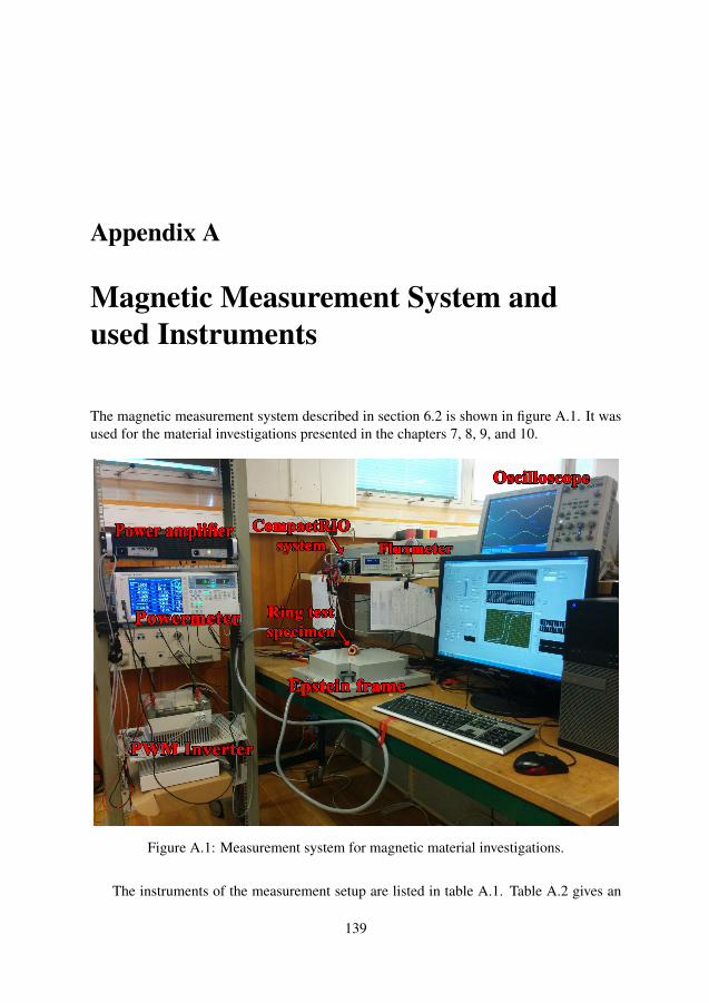
Appendix A
Magnetic Measurement System and
used Instruments
The magnetic measurement system described in section 6.2 is shown in figure A.1. It wasused for the material investigations presented in the chapters 7, 8, 9, and 10.
Figure A.1: Measurement system for magnetic material investigations.
The instruments of the measurement setup are listed in table A.1. Table A.2 gives an
139
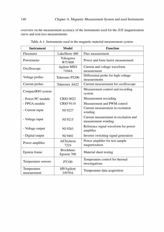
140 Chapter A. Magnetic Measurement System and used Instruments
overview on the measurement accuracy of the instruments used for the BH magnetizationcurve and iron loss measurements.
Table A.1: Instruments used in the magnetic material measurement system.
Instrument Model Function
Fluxmeter LakeShore 480 Flux measurement
PowermeterYokogawaWT1800
Power and form factor measurement
Oscilloscope Agilent MSO7104A
Current and voltage waveformmeasurement
Voltage probes Tektronix P5200Differential probe for high voltagemeasurements
Current probes Tektronix A622 Current measurement for oscilloscope
CompactRIO systemMeasurement control and recordingsystem
- Power PC module CRIO 9022 Measurement recording
- FPGA module CRIO 9114 Measurement and PWM control
- Current input NI 9227Current measurement in excitationwinding
- Voltage input NI 9215Current measurement in excitation andmeasurement winding
- Voltage output NI 9263Reference signal waveform for poweramplifier
- Digital output NI 9401 Inverter switching signal generation
Power amplifier AETechron7224
Power amplifier for test samplemagnetization
Epstein frameBrockhausEpstein 700
Material sheet testing
Temperature sensors PT100Temperature control for thermalinvestigations
Temperaturemeasurement
HP/Agilent34970A
Temperature data acquisition

141
Table A.2: Datasheet specifications of used measurement instruments.
InstrumentMeasurement
RangeAccuracy
Yokogawa WT1800power meter
- Voltage measurement 1.5 V to 1 kVbetter than ± (0.1 % of reading + 0.1 %of range) at 10 Hz to 1 kHz
- Current measurement 10 mA to 5 Abetter than ± (0.1 % of reading + 0.1 %of range) at 10 Hz to 1 kHz
- Power measurementdepending onvoltage and
current range
better than ± (0.2 % of reading + 0.1 %of range) at 10 Hz to 1 kHz
LakeShore 480 fluxmeter
30 mVs or300 mVs
better than ± (0.25 % of reading +[10 µVs and 1 µVs/min] offset and drift)
NI 9227 current module 5 Abetter than ± (0.37 % of reading +0.18 % of range)
NI 9215 voltage module 10.4 Vbetter than ± (0.2 % of reading +0.082 % of range)
Tektronix P5200voltage probe 130 V or 1.3 kV
better than ± (3 % of range) at DC to100 kHz
Tektronix A622 currentprobe 10 A or 100 A
better than ± (3 % of reading + 50 mA)at DC to 1 kHz

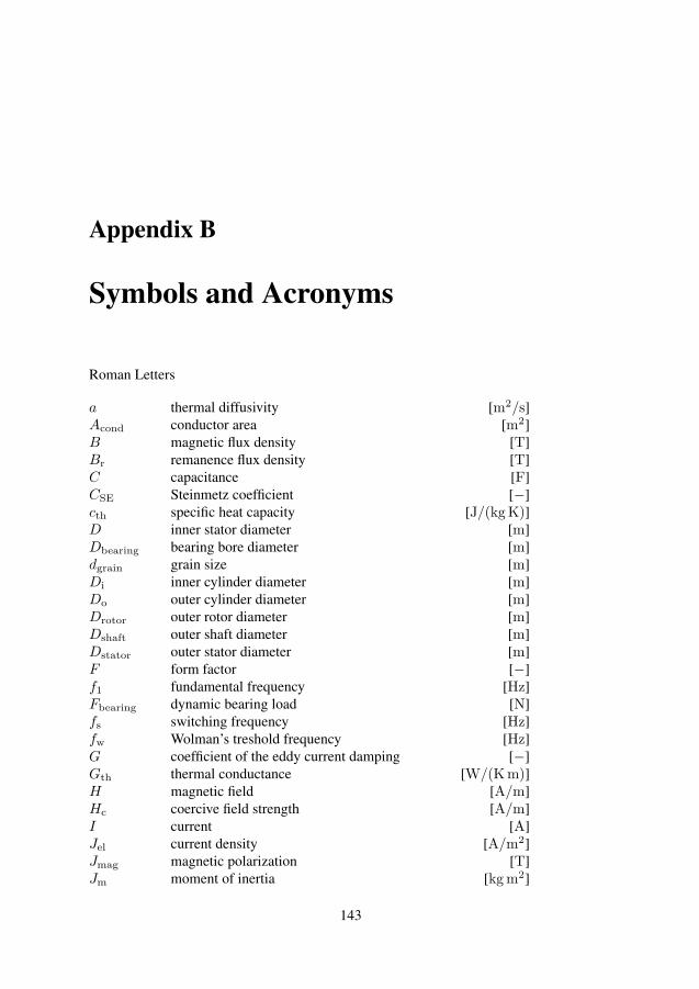
Appendix B
Symbols and Acronyms
Roman Letters
a thermal diffusivity [m2/s]Acond conductor area [m2]B magnetic flux density [T]Br remanence flux density [T]C capacitance [F]CSE Steinmetz coefficient [−]cth specific heat capacity [J/(kg K)]D inner stator diameter [m]Dbearing bearing bore diameter [m]dgrain grain size [m]Di inner cylinder diameter [m]Do outer cylinder diameter [m]Drotor outer rotor diameter [m]Dshaft outer shaft diameter [m]Dstator outer stator diameter [m]F form factor [−]f1 fundamental frequency [Hz]Fbearing dynamic bearing load [N]fs switching frequency [Hz]fw Wolman’s treshold frequency [Hz]G coefficient of the eddy current damping [−]Gth thermal conductance [W/(K m)]H magnetic field [A/m]Hc coercive field strength [A/m]I current [A]Jel current density [A/m2]Jmag magnetic polarization [T]Jm moment of inertia [kg m2]
143
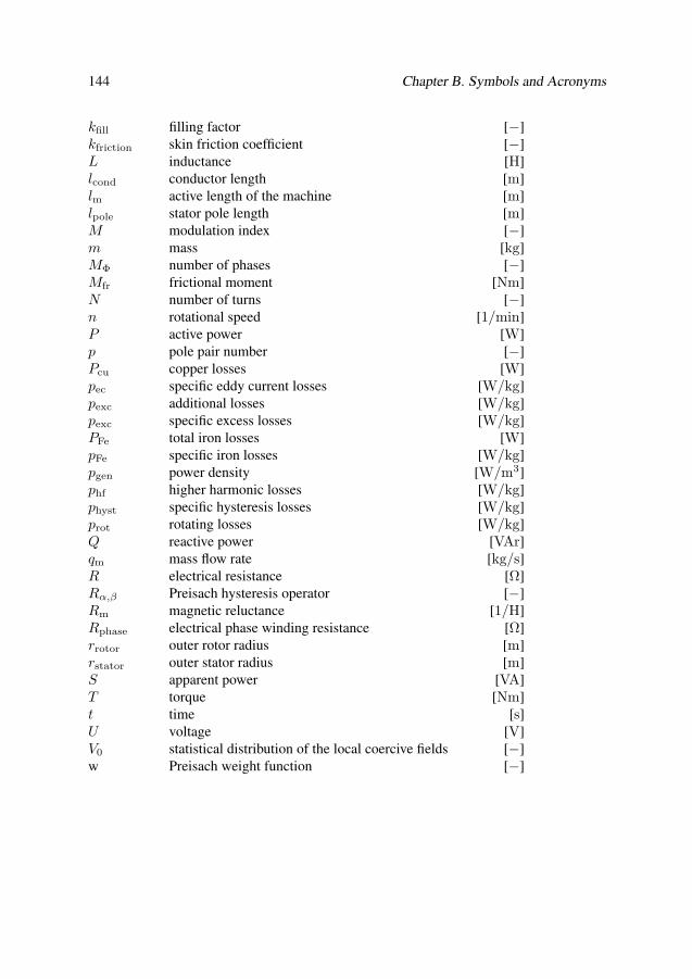
144 Chapter B. Symbols and Acronyms
kfill filling factor [−]kfriction skin friction coefficient [−]L inductance [H]lcond conductor length [m]lm active length of the machine [m]lpole stator pole length [m]M modulation index [−]m mass [kg]MΦ number of phases [−]Mfr frictional moment [Nm]N number of turns [−]n rotational speed [1/min]P active power [W]p pole pair number [−]Pcu copper losses [W]pec specific eddy current losses [W/kg]pexc additional losses [W/kg]pexc specific excess losses [W/kg]PFe total iron losses [W]pFe specific iron losses [W/kg]pgen power density [W/m3]phf higher harmonic losses [W/kg]physt specific hysteresis losses [W/kg]prot rotating losses [W/kg]Q reactive power [VAr]qm mass flow rate [kg/s]R electrical resistance [Ω]Rα,β Preisach hysteresis operator [−]Rm magnetic reluctance [1/H]Rphase electrical phase winding resistance [Ω]rrotor outer rotor radius [m]rstator outer stator radius [m]S apparent power [VA]T torque [Nm]t time [s]U voltage [V]V0 statistical distribution of the local coercive fields [−]w Preisach weight function [−]

145
Greek Letters
α Steinmetz coefficient [−]αcu copper temperature coefficient [−]β Steinmetz coefficient [−]δ airgap length [m]δs skin depth [m]η efficiency [−]γ mass density [kg/m3]µ0 permeability of vacuum [V s/(A m)]µa amplitude permeability [−]µfr friction coefficient [−]µi initial permeability [−]µmax maximum permeability [−]µr relative magnetic permeability [−]ωel electrical angular frequency [Hz]ωm mechanical angular frequency [Hz]Ψ magnetic flux [Wb]ρ electrical resistivity [Ω m]σ electrical conductivity [S/m]σth thermal conductivity [W K/m]θ rotor position [−]ϕ phase angle [rad]ϑ temperature [C]
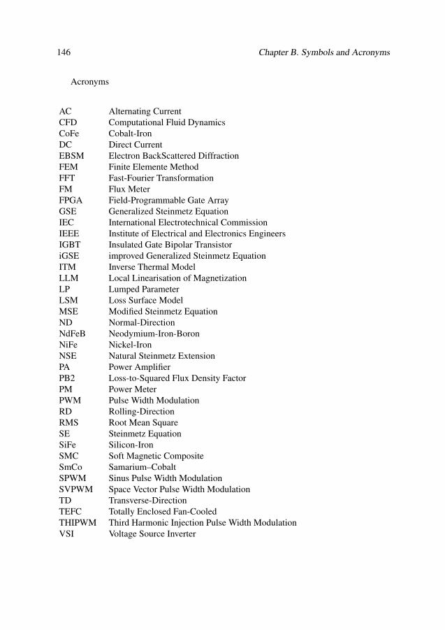
146 Chapter B. Symbols and Acronyms
Acronyms
AC Alternating CurrentCFD Computational Fluid DynamicsCoFe Cobalt-IronDC Direct CurrentEBSM Electron BackScattered DiffractionFEM Finite Elemente MethodFFT Fast-Fourier TransformationFM Flux MeterFPGA Field-Programmable Gate ArrayGSE Generalized Steinmetz EquationIEC International Electrotechnical CommissionIEEE Institute of Electrical and Electronics EngineersIGBT Insulated Gate Bipolar TransistoriGSE improved Generalized Steinmetz EquationITM Inverse Thermal ModelLLM Local Linearisation of MagnetizationLP Lumped ParameterLSM Loss Surface ModelMSE Modified Steinmetz EquationND Normal-DirectionNdFeB Neodymium-Iron-BoronNiFe Nickel-IronNSE Natural Steinmetz ExtensionPA Power AmplifierPB2 Loss-to-Squared Flux Density FactorPM Power MeterPWM Pulse Width ModulationRD Rolling-DirectionRMS Root Mean SquareSE Steinmetz EquationSiFe Silicon-IronSMC Soft Magnetic CompositeSmCo Samarium–CobaltSPWM Sinus Pulse Width ModulationSVPWM Space Vector Pulse Width ModulationTD Transverse-DirectionTEFC Totally Enclosed Fan-CooledTHIPWM Third Harmonic Injection Pulse Width ModulationVSI Voltage Source Inverter
List of Figures
2.1 Basic structure of a permanent magnet machine. . . . . . . . . . . . . . 102.2 Typical efficiency and loss values of a a) 110 kW permanent magnet
high-speed generator (51 000 rpm) [7], b) 11 kW induction machine (1470 rpm)[8], c) 1 kW slot-less permanent magnet motor for hand tools (36 000 rpm).
112.3 General loss separation in electrical machines. . . . . . . . . . . . . . . 112.4 BH hysteresis curve of a ferromagnetic material at 10 Hz (red) and
200 Hz (blue). . . . . . . . . . . . . . . . . . . . . . . . . . . . . . . . 15
3.1 Influencing factors of the manufacturing process of electrical machinecores. . . . . . . . . . . . . . . . . . . . . . . . . . . . . . . . . . . . 21
4.1 Model approaches to determine iron losses in electrical machines. . . . 264.2 Preisach model overview with hysteresis operator Rα,β and weight func-
tions w1,2,...,n. . . . . . . . . . . . . . . . . . . . . . . . . . . . . . . 32
5.1 Magnetic domains (coloured areas) and domain walls (black lines) of aNiFe lamination sample1. . . . . . . . . . . . . . . . . . . . . . . . . . 38
5.2 Initial BH magnetization curve and its effects on the magnetic domains. 395.3 Machine operating points on the initial hysteresis magnetization curve. . 435.4 Loss-to-squared flux density factor PB2 for typical electrical machine
materials. . . . . . . . . . . . . . . . . . . . . . . . . . . . . . . . . . 44
6.1 Magnetic measurement methods to determine magnetic properties andiron losses in lamination sheets for electrical machines. . . . . . . . . . 48
6.2 Overview on the measurement setup, where solid lines indicate the elec-tric power circuit and dashed lines the measurement and data flow. . . . 49
6.3 Typical demagnetization curve of a ring core test specimen. . . . . . . . 506.4 Initial magnetization curve with a constant dB/dt of 0.02 T/s . . . . . . 516.5 Flow chart of the AC measurements control system. . . . . . . . . . . . 526.6 Flow chart of the iterative control system algorithm. . . . . . . . . . . . 536.7 LabVIEW user interface of the AC measurement system. . . . . . . . . 54
147
148 List of Figures
6.8 Overview on the measurement setup for PWM excitation. Solid linesindicate the electric power circuit and dashed lines the measurement anddata flow. . . . . . . . . . . . . . . . . . . . . . . . . . . . . . . . . . 55
6.9 Regular sampled symmetric signal of the PWM measurement systemwith a modulation index of 0.7. . . . . . . . . . . . . . . . . . . . . . . 55
7.1 Investigated stator core with stranded wire excitation winding. . . . . . 617.2 Axial welding seam of a SiFe stator core (top) and a 0.1 mm NiFe stator
core (bottom). . . . . . . . . . . . . . . . . . . . . . . . . . . . . . . . 627.3 Magnified welding seams of 0.2 mm NiFe and SiFe stator cores. . . . . 637.4 Initial BH magnetization curves up to a magnetic field peak value of
H = 3000 A/m. . . . . . . . . . . . . . . . . . . . . . . . . . . . . . 637.5 Amplitude permeability µr of the non-welded and welded stator cores. . 647.6 BH hysteresis loops from Epstein frame test and SiFe ring core mea-
surements before and after the welding process at 50 Hz and a magneticflux density peak value of B = 0.7 T. . . . . . . . . . . . . . . . . . . 65
7.7 Welded and non-welded NiFe BH hysteresis loops at 50 Hz and a mag-netic flux density peak value of B = 1.2 T. . . . . . . . . . . . . . . . 66
7.8 Magnetic coercivity of the four investigated NiFe cores (Magnificationof the grey rectangle in figure 7.7). . . . . . . . . . . . . . . . . . . . . 67
7.9 Specific iron losses p over the magnetic flux density for SiFe and NiFeat 50 Hz. . . . . . . . . . . . . . . . . . . . . . . . . . . . . . . . . . . 67
7.10 Specific iron losses p over the magnetic flux density for SiFe and NiFeat 200 Hz. . . . . . . . . . . . . . . . . . . . . . . . . . . . . . . . . . 68
7.11 Specific iron losses over frequency at a maximum magnetic flux densitypeak value of B = 1.4 T. . . . . . . . . . . . . . . . . . . . . . . . . . 68
7.12 Specific iron losses per cycle for NiFe at a maximum magnetic flux den-sity peak value of B = 1.4 T. . . . . . . . . . . . . . . . . . . . . . . . 69
7.13 Iron loss reduction when exchanging 0.2 mm SiFe with 0.2 mm NiFe forBmax = 1.4 T. . . . . . . . . . . . . . . . . . . . . . . . . . . . . . . 70
7.14 Flux density distribution in the wound stator core. . . . . . . . . . . . . 717.15 Measured (markers) and modelled (lines) iron losses for the SiFe stator
cores. . . . . . . . . . . . . . . . . . . . . . . . . . . . . . . . . . . . 727.16 Discrepancies between measured and modelled iron losses for the SiFe
stator cores. . . . . . . . . . . . . . . . . . . . . . . . . . . . . . . . . 737.17 Discrepancies between measured and modelled iron losses for the 0.1 mm
NiFe stator cores. . . . . . . . . . . . . . . . . . . . . . . . . . . . . . 737.18 2D FEM model of the investigated PMSM. . . . . . . . . . . . . . . . 747.19 Equipotential lines in the investigated PMSM at full load. . . . . . . . . 757.20 Flux density in the stator core for the circumferential and radial direction
at full load. . . . . . . . . . . . . . . . . . . . . . . . . . . . . . . . . 767.21 Ratio of rotational to alternating flux density distribution in the stator
core in percent. . . . . . . . . . . . . . . . . . . . . . . . . . . . . . . 77
List of Figures 149
8.1 Thermal test chamber with ring core test specimen. . . . . . . . . . . . 808.2 Initial magnetizing curve for 0.1 mm and 0.2 mm NiFe lamination sheets
with a constant dB/dt. . . . . . . . . . . . . . . . . . . . . . . . . . . . 818.3 Complete BH hysteresis curves for 0.2 mm lamination sheets at 100 Hz
and a maximum flux density of 1.3 T. . . . . . . . . . . . . . . . . . . 828.4 Zoom of the coercitivity field from figure 8.3. . . . . . . . . . . . . . . 828.5 Specific iron losses in the 0.2 mm stator core for different sinusoidal flux
densities at 100 Hz. . . . . . . . . . . . . . . . . . . . . . . . . . . . . 838.6 Electrical output torque of the PMSM as a function of on the stator core
and permanent magnet temperature (simulated points marked with ’X’). 848.7 Magnetic flux density distribution for a constant operating point at min-
imum temperature (left) and maximum temperature (right). . . . . . . . 85
9.1 Current waveform of the PWM voltage in the primary winding with abase frequency of 50 Hz. . . . . . . . . . . . . . . . . . . . . . . . . . 88
9.2 BH hysteresis loop of the welded SiFe stator core at 50 Hz base fre-quency and a fundamental flux density peak value of 1.2 T. . . . . . . . 89
9.3 BH hysteresis loop of the welded NiFe stator core at 50 Hz base fre-quency and a fundamental flux density peak value of 1.4 T. . . . . . . . 90
9.4 Magnification of the welded SiFe BH hysteresis loop from figure 9.2around zero flux density (grey rectangle). . . . . . . . . . . . . . . . . 91
9.5 Magnification of the welded NiFe BH hysteresis loop from figure 9.3around zero flux density (grey rectangle). . . . . . . . . . . . . . . . . 91
9.6 Iron losses in the welded SiFe stator core at a base frequency of 50 Hzand fundamental flux density peak values of 1 T and 1.4 T, respectively. 92
9.7 Iron losses in the welded SiFe stator core at a base frequency of 200 Hzand a fundamental flux density peak value of 1 T and 1.4 T, respectively. 92
9.8 Iron losses in the welded NiFe stator core at base frequencies of 50 Hzand 200 Hz and a fundamental flux density peak value of 1.4 T, respectively. 93
9.9 Iron loss increase (PWM/sinusoidal) in the welded SiFe stator core at abase frequency of 50 Hz related to pure sinusoidal flux density iron losses. 94
9.10 Iron loss increase (PWM/sinusoidal) in the welded SiFe stator core at abase frequency of 200 Hz related to pure sinusoidal flux density iron losses. 95
9.11 Iron loss increase (PWM/sinusoidal) in the welded NiFe stator core re-lated to pure sinusoidal flux density iron losses at 1.4 T. . . . . . . . . . 95
9.12 Relative core loss increase between the welded and non-welded SiFeand NiFe stator cores at different modulation indices and a magnetic fluxdensity peak value of 1.4 T. . . . . . . . . . . . . . . . . . . . . . . . . 96
9.13 Line-to-line voltage and phase current in the PWM FEM simulation. . . 979.14 Torque comparison between PWM and sinusoidal voltage excitation. . . 989.15 Third period of the torque comparison between PWM and sinusoidal
voltage excitation. . . . . . . . . . . . . . . . . . . . . . . . . . . . . . 999.16 Torque ripple comparison for PWM operation at 5 kHz and 20 kHz switch-
ing frequency. . . . . . . . . . . . . . . . . . . . . . . . . . . . . . . . 99
150 List of Figures
9.17 Torque ripple comparison for PWM operation at modulation indices of0.5 and 0.9 at 5 kHz switching frequency. . . . . . . . . . . . . . . . . 100
9.18 Flux density distribution of the 23rd harmonic in the stator core of thePWM simulation case at 5 kHz switching frequency and a modulationindex of 0.9. . . . . . . . . . . . . . . . . . . . . . . . . . . . . . . . . 101
9.19 Iron loss dependency on the modulation index. . . . . . . . . . . . . . 102
10.1 Stacked CoFe stator core during the winding process with the inner mea-surement winding in the slots (white) and outer excitation winding (brown)around the teeth and yoke. . . . . . . . . . . . . . . . . . . . . . . . . 105
10.2 Annealed NiFe stator core during the winding process with inner mea-surement winding (yellow) and outer excitation winding (stranded cop-per wire). . . . . . . . . . . . . . . . . . . . . . . . . . . . . . . . . . 105
10.3 Grain structure of CoFe lamination sheets from sample A, B and C, sideview at 500x magnification. . . . . . . . . . . . . . . . . . . . . . . . . 107
10.4 Grain structure of CoFe lamination sheets from sample A, B and C, topview at 200x magnification. . . . . . . . . . . . . . . . . . . . . . . . . 108
10.5 Grain structure of the NiFe sheet’s short side before and after the anneal-ing process. . . . . . . . . . . . . . . . . . . . . . . . . . . . . . . . . 109
10.6 Grain structure of the NiFe sheet’s long side before and after the anneal-ing process. . . . . . . . . . . . . . . . . . . . . . . . . . . . . . . . . 109
10.7 Initial BH magnetization curve of the three CoFe stator cores. . . . . . 11010.8 Iron losses of the three CoFe stator cores at 50 Hz. . . . . . . . . . . . 11110.9 Initial BH magnetization curve of the four NiFe stator cores. . . . . . . 11210.10 Demagnetization curves of the non-annealed laser cut NiFe stator core
with different demagnetization starting points. . . . . . . . . . . . . . . 11310.11 Initial BH magnetization curves of the non-annealed laser cut NiFe sta-
tor core after different demagnetization starting points as shown in fig-ure 10.10. . . . . . . . . . . . . . . . . . . . . . . . . . . . . . . . . . 113
10.12 Quasi-static full BH hysteresis loops of the annealed and non-annealedlaser cut NiFe stator cores with a maximum flux density of 1.1 T. . . . . 114
10.13 Specific iron losses of the the annealed and non-annealed laser cut andpunched NiFe stator cores. . . . . . . . . . . . . . . . . . . . . . . . . 114
10.14 Full BH hysteresis loop of the annealed stator cores at 50 Hz and a max-imum flux density of 1.3 T. . . . . . . . . . . . . . . . . . . . . . . . . 115
10.15 Magnification of the full BH hysteresis loop from figure 10.14 aroundzero flux density (grey rectangle). . . . . . . . . . . . . . . . . . . . . 116
11.1 Lumped parameter model of the investigated outer-rotor PMSM in Motor-CAD. . . . . . . . . . . . . . . . . . . . . . . . . . . . . . . . . . . . 118
11.2 Stator and rotor with axial cooling ducts of the investigated outer-rotorPMSM. . . . . . . . . . . . . . . . . . . . . . . . . . . . . . . . . . . 120
11.3 The machine model in Motor-CAD, front and axial view. . . . . . . . . 12111.4 Transient temperature graph for 20 W rotor losses. . . . . . . . . . . . 123
List of Figures 151
11.5 Transient temperature graph for 50 W total losses in the stator. . . . . . 12311.6 Transient temperature graph for 60 W copper losses in the winding and
60 W iron losses in the stator and rotor. . . . . . . . . . . . . . . . . . 12411.7 Stator tooth tips (green) and stator tooth yoke (violet) of the FEM model. 12511.8 Iron loss density (surface contour in W/kg) and current density vectors
at no-load, 700 rpm. . . . . . . . . . . . . . . . . . . . . . . . . . . . . 12611.9 Thermal measurement setup of the investigated outer-rotor PMSM. . . . 12711.10 PT100 temperature sensors mounted on the front side of the stator tooth
tip and on the winding coil. . . . . . . . . . . . . . . . . . . . . . . . . 12811.11 Thermal image of the stator coils and mounted PT100 sensors at a no-
load test with 700 rpm. . . . . . . . . . . . . . . . . . . . . . . . . . . 12811.12 Temperature rises of sensor 1 (S1) and sensor 3 (S3) at no-load condition
for 300 rpm, 500 rpm, and 700 rpm. . . . . . . . . . . . . . . . . . . . 12911.13 Initial temperature rise of sensor 1 for 300 rpm, 500 rpm, and 700 rpm. . 13011.14 Iron loss density in the stator tooth tips determined by FEM simulations
and thermal measurements for 300 rpm, 500 rpm, and 700 rpm. . . . . . 131
A.1 Measurement system for magnetic material investigations. . . . . . . . 139

Bibliography
[1] International Energy Agency, World energy outlook, Organisation for EconomicCo-operation and Development, Paris, France, Report Number 1026-1141, 2013.
[2] B. Mecrow and A. Jack, “Efficiency trends in electric machines and drives,” Energy
Policy, vol. 36, no. 12, pp. 4336–4341, 2008.
[3] “Commission regulation (EC) no 640/2009 of 22 july 2009 implementing directive2005/32/EC of the european parliament and of the council with regard to ecodesignrequirements for electric motors,” Official Journal of the European Union, vol. 52,2009.
[4] Rotating electrical machines - part 30-1: efficiency classes of line operated AC
motors (IE code), International Standard IEC 60034-30-1, 2014.
[5] A. de Almeida, F. Ferreira, and J. Fong, “Standards for efficiency of electric mo-tors,” IEEE Industry Applications Magazine, vol. 17, no. 1, pp. 12–19, 2011.
[6] C. T. Liu, L. Y. Liu, and S. Y. Lin, “Electromagnetic steel products: a systematiciron loss evaluating scheme,” IEEE Industry Applications Magazine, vol. 18, no.1, pp. 27–33, 2012.
[7] O. Aglen, “Loss calculation and thermal analysis of a high-speed generator,” inIEEE International Electric Machines and Drives Conference (IEMDC), vol. 2,Madison, USA, 2003, pp. 1117–1123.
[8] A. Krings, S. Nategh, A. Stening, H. Grop, O. Wallmark, and J. Soulard, “Mea-surement and modeling of iron losses in electrical machines,” in 5th International
Conference Magnetism and Metallurgy (WMM), Gent, Belgium, 2012, pp. 101–119.
[9] Rolling bearings and seals in electric motors and generators. SKF Group, 2013.
[10] Rolling bearings - SKF Broschure. SKF Group, 2012.
[11] T. A. Harris and M. N. Kotzalas, Advanced Concepts of Bearing Technology -
Rolling Bearing Analysis, 5th ed. CRC Press, 2006, ISBN: 9780849371837.
[12] J. E. Vrancik, Prediction of windage power loss in alternators, NASA technicalnote TN D-4849, 1968.
[13] J. Saari, “Thermal analysis of high-speed induction machines,” PhD thesis, AaltoUniversity, Helsinki, Finland, 1998.
153
154 BIBLIOGRAPHY
[14] E. Bilgen and R. Boulos, “Functional dependence of torque coefficient of coaxialcylinders on gap width and Reynolds numbers,” Journal of Fluids Engineering,vol. 95, no. 1, pp. 122–126, 1973.
[15] J. W. Polkowski, “Turbulent flow between coaxial cylinders with the inner cylinderrotating,” Journal of Engineering for Gas Turbines and Power, vol. 106, no. 1,pp. 128–135, 1984.
[16] J. Pyrhönen, T. Jokinen, and V. Hrabovcova, Design of Rotating Electrical Ma-
chines. John Wiley & Sons, 2009, ISBN: 9780470740088.
[17] F. Magnussen, “On design and analysis of synchronous permanent magnet ma-chines for field-weakening operation in hybrid electric vehicles,” PhD thesis, KTHRoyal Institute of Technology, Stockholm, Sweden, 2004.
[18] M. Popescu and D. Dorrell, “Skin effect and proximity losses in high speed brush-less permanent magnet motors,” in IEEE Energy Conversion Congress and Expo-
sition (ECCE), 2013, pp. 3520–3527.
[19] Magnetic materials - part 1-1: classification, International Standard IEC 60404-1:2000.
[20] Standard specification for nonoriented electrical steel fully processed types, ASTMInternational, A677, 2012.
[21] M. Oka, M. Kawano, K. Shimada, T. Kai, and M. Enokizono, “Evaluation of themagnetic properties of the rotating machines for the building factor clarification,”Przeglad Elektrotechniczny (Electrical Review), vol. 87, no. 9, pp. 43–46, 2011.
[22] P. Hargreaves, B. Mecrow, and R. Hall, “Calculation of iron loss in electrical gen-erators using finite-element analysis,” IEEE Transactions on Industry Applications,vol. 48, no. 5, pp. 1460–1466, 2012.
[23] W. Roshen, “Iron loss model for permanent-magnet synchronous motors,” IEEE
Transactions on Magnetics, vol. 43, no. 8, pp. 3428–3434, 2007.
[24] A. Jack, B. Mecrow, P. Dickinson, D. Stephenson, J. Burdess, N. Fawcett, and J. T.Evans, “Permanent-magnet machines with powdered iron cores and prepressedwindings,” IEEE Transactions on Industry Applications, vol. 36, no. 4, pp. 1077–1084, 2000.
[25] Methods of measurement of the magnetic properties of electrical steel strip and
sheet by means of an Epstein frame., International Standard IEC 60404-2:2008.
[26] Test method for alternating current magnetic properties of materials using the
wattmeter-ammeter-voltmeter method, 100 to 10 000 hz and 25-cm Epstein frame,ASTM International, A348 / A348M, 2011.
[27] Test method for alternating-current magnetic properties of materials at power
frequencies using wattmeter-ammeter-voltmeter method and 25-cm Epstein test
frame, ASTM International, A343 / A343M, 2008.

BIBLIOGRAPHY 155
[28] Methods of measurement of the magnetic properties of magnetically soft metallic
and powder materials at frequencies in the range 20Hz to 200kHz by the use of
ring specimens, International Standard IEC 60404-6:2003.
[29] H. Ahlers and J. Lüdke, “The uncertainties of magnetic properties measurementsof electrical sheet steel,” Journal of Magnetism and Magnetic Materials, vol. 215-216, pp. 711–713, 2000.
[30] Rotating electrical machines - part 2-1: standard methods for determining losses
and efficiency from tests (excluding machines for traction vehicles), InternationalStandard IEC 60034-2-1, 2007.
[31] IEEE guide: test procedures for synchronous machines, 1995.
[32] C. Steinmetz, “On the law of hysteresis (originally published in 1892),” Proceed-
ings of the IEEE, vol. 72, no. 2, pp. 197–221, 1984.
[33] C. D. Graham, “Physical origin of losses in conducting ferromagnetic materials,”Journal of Applied Physics, vol. 53, no. 11, pp. 8276–8280, 1982.
[34] R. Hilzinger and W. Rodewald, Magnetic materials fundamentals, products, prop-
erties, applications. Erlangen: Publicis, 2013, ISBN: 9783895783524.
[35] N. Takahashi, H. Morimoto, Y. Yunoki, and D. Miyagi, “Effect of shrink fittingand cutting on iron loss of permanent magnet motor,” Journal of Magnetism and
Magnetic Materials, vol. 320, no. 20, pp. 925–928, 2008.
[36] F. Henrotte, J. Schneider, and K. Hameyer, “Influence of the manufacturing pro-cess in the magnetic properties of iron cores in induction machines,” in 2nd Inter-
national Workshop Magnetism and Metallurgy (WMM), Freiberg, Germany, 2006.
[37] R. Rygal, A. J. Moses, N. Derebasi, J. Schneider, and A. Schoppa, “Influence ofcutting stress on magnetic field and flux density distribution in non-oriented electri-cal steels,” Journal of Magnetism and Magnetic Materials, vol. 215-216, pp. 687–689, 2000.
[38] A. Schoppa, J. Schneider, and J. O. Roth, “Influence of the cutting process on themagnetic properties of non-oriented electrical steels,” Journal of Magnetism and
Magnetic Materials, vol. 215-216, pp. 100–102, 2000.
[39] T. Nakata, M. Nakano, and K. Kawahara, “Effects of stress due to cutting on mag-netic characteristics of silicon steel,” IEEE Translation Journal on Magnetics in
Japan, vol. 7, no. 6, pp. 453–457, 1992.
[40] A. J. Moses, N. Derebasi, G. Loisos, and A. Schoppa, “Aspects of the cut-edge ef-fect stress on the power loss and flux density distribution in electrical steel sheets,”Journal of Magnetism and Magnetic Materials, vol. 215-216, pp. 690–692, 2000.
[41] J. Schneider, Magnetische Werkstoffe und Anwendungen. Lecture notes from RWTHAachen University, 2008.
156 BIBLIOGRAPHY
[42] Z. Gmyrek, A. Cavagnino, and L. Ferraris, “Estimation of the magnetic propertiesof the damaged area resulting from the punching process: experimental researchand FEM modeling,” IEEE Transactions on Industry Applications, vol. 49, no. 5,pp. 2069–2077, 2013.
[43] A. Kedous-Lebouc, B. Cornut, J. C. Perrier, P. Manfé, and T. Chevalier, “Punchinginfluence on magnetic properties of the stator teeth of an induction motor,” Journal
of Magnetism and Magnetic Materials, vol. 254-255, pp. 124–126, 2003.
[44] Y. Liu, S. K. Kashif, and A. M. Sohail, “Engineering considerations on additionaliron losses due to rotational fields and sheet cutting,” in 18th International Confer-
ence on Electrical Machines (ICEM), Vilamoura, Portugal, 2008, pp. 1–4.
[45] W. Arshad, T. Ryckebusch, F. Magnussen, H. Lendenmann, B. Eriksson, J. Soulard,and B. Malmros, “Incorporating lamination processing and component manufac-turing in electrical machine design tools,” in 42nd IAS Annual Meeting Industry
Applications Conference, vol. 1, 2007, pp. 94–102.
[46] A. Boglietti, A. Cavagnino, L. Ferraris, and M. Lazzari, “The annealing influ-ence onto the magnetic and energetic properties in soft magnetic material afterpunching process,” in IEEE International Electric Machines and Drives Confer-
ence (IEMDC), vol. 1, Madison, USA, 2003, pp. 503–508.
[47] M. Emura, F. J. G. Landgraf, W. Ross, and J. R. Barreta, “The influence of cuttingtechnique on the magnetic properties of electrical steels,” Journal of Magnetism
and Magnetic Materials, vol. 254-255, pp. 358–360, 2003.
[48] A. Schoppa, J. Schneider, C. D. Wuppermann, and T. Bakon, “Influence of weld-ing and sticking of laminations on the magnetic properties of non-oriented electri-cal steels,” Journal of Magnetism and Magnetic Materials, vol. 254, pp. 367–369,2003.
[49] A. Schoppa, J. Schneider, and C. D. Wuppermann, “Influence of the manufacturingprocess on the magnetic properties of non-oriented electrical steels,” Journal of
Magnetism and Magnetic Materials, vol. 215, pp. 74–78, 2000.
[50] P. Beckley, Electrical Steels for Rotating Machines. The Institution of Engineeringand Technology, 2002, ISBN: 0852969805.
[51] M. Fratila, R. Ramarotafika, A. Benabou, S. Clénet, and A. Tounzi, “Stochasticpost-processing calculation of iron losses – application to a PMSM,” COMPEL:
The International Journal for Computation and Mathematics in Electrical and
Electronic Engineering, vol. 32, no. 4, pp. 1383–1392, 2013.
[52] J. Tangudu, T. Jahns, and A. EL-Refaie, “Core loss prediction using magnetic cir-cuit model for fractional-slot concentrated-winding interior permanent magnet ma-chines,” in IEEE Energy Conversion Congress and Exposition (ECCE), Atlanta,USA, 2010.
[53] J. Reinert, A. Brockmeyer, and R. De Doncker, “Calculation of losses in ferro- andferrimagnetic materials based on the modified Steinmetz equation,” IEEE Trans-
actions on Industry Applications, vol. 37, no. 4, pp. 1055–1061, 2001.
BIBLIOGRAPHY 157
[54] A. Brockmeyer, “Dimensionierungswerkzeug für magnetische bauelemente in strom-richteranwendungen,” PhD thesis, RWTH Aachen University, Aachen, Germany,1997.
[55] J. Li, T. Abdallah, and C. Sullivan, “Improved calculation of core loss with nonsi-nusoidal waveforms,” in 36th IAS Annual Meeting Industry Applications Confer-
ence, vol. 4, 2001, pp. 2203–2210.
[56] K. Venkatachalam, C. Sullivan, T. Abdallah, and H. Tacca, “Accurate prediction offerrite core loss with nonsinusoidal waveforms using only Steinmetz parameters,”in IEEE Workshop on Computers in Power Electronics, 2002, pp. 36–41.
[57] A. Van den Bossche, V. Valchev, and G. Georgiev, “Measurement and loss modelof ferrites with non-sinusoidal waveforms,” in IEEE 35th Annual Power Electron-
ics Specialists Conference (PESC), vol. 6, 2004, pp. 4814–4818.
[58] H. Jordan, “Die ferromagnetischen konstanten für schwache wechselfelder,” Elek-
trische Nachrichtentechnik, vol. 1, p. 8, 1924.
[59] R. Boll, Weichmagnetische Werkstoffe, 4th ed. Vacuumschmelze GmbH, Hanau,Germany, 1990, ISBN: 3800915464.
[60] R. H. Pry and C. P. Bean, “Calculation of the energy loss in magnetic sheet materi-als using a domain model,” Journal of Applied Physics, vol. 29, no. 3, pp. 532–533,1958.
[61] G. Bertotti, “Physical interpretation of eddy current losses in ferromagnetic ma-terials. I. theoretical considerations,” Journal of Applied Physics, vol. 57, no. 6,pp. 2110–2117, 1985.
[62] G. Bertotti, “Physical interpretation of eddy current losses in ferromagnetic mate-rials. II. analysis of experimental results,” Journal of Applied Physics, vol. 57, no.6, pp. 2118–2126, 1985.
[63] G. Bertotti, G. Di Schino, A. Ferro Milone, and F. Fiorillo, “On the effect of grainsize on magnetic losses of 3% non-oriented SiFe,” Le Journal de Physique Collo-
ques, vol. 46, no. 6, p. 385, 1985.
[64] F. Fiorillo and A. Novikov, “An improved approach to power losses in magneticlaminations under nonsinusoidal induction waveform,” IEEE Transactions on Mag-
netics, vol. 26, no. 5, pp. 2904–2910, 1990.
[65] Flux 10 - 2D/3D Applications User’s Guide. Meylan, France: Cedrat Group, 2007.
[66] “Estimating iron loss in opera-2d,” in Opera-2d User Guide, Oxfordshire, UK:Cobham Technical Services, 2012.
[67] JMAG version 10 - User’s manual. Tokyo, Japan: JSOL Cooperation, 2010.
[68] G. Bertotti, “General properties of power losses in soft ferromagnetic materials,”IEEE Transactions on Magnetics, vol. 24, no. 1, pp. 621–630, 1988.
[69] W. A. Pluta, “Some properties of factors of specific total loss components in elec-trical steel,” IEEE Transactions on Magnetics, vol. 46, no. 2, pp. 322–325, 2010.
158 BIBLIOGRAPHY
[70] A. Moses, “Importance of rotational losses in rotating machines and transformers,”Journal of Materials Engineering and Performance, vol. 1, no. 2, pp. 235–244,1992.
[71] K. Atallah and D. Howe, “Calculation of the rotational power loss in electrical steellaminations from measured H and B,” IEEE Transactions on Magnetics, vol. 29,no. 6, pp. 3547–3549, 1993.
[72] T. Kochmann, “Relationship between rotational and alternating losses in electricalsteel sheets,” Journal of Magnetism and Magnetic Materials, vol. 160, pp. 145–146, 1996.
[73] N. Stranges and R. Findlay, “Measurement of rotational iron losses in electricalsheet,” IEEE Transactions on Magnetics, vol. 36, no. 5, pp. 3457–3459, 2000.
[74] F. Fiorillo and A. M. Rietto, “Rotational versus alternating hysteresis losses innonoriented soft magnetic laminations,” in 37th Annual conference on magnetism
and magnetic materials, vol. 73, Houston, USA, 1993, pp. 6615–6617.
[75] Y. Guo, J. G. Zhu, J. Zhong, H. Lu, and J. X. Jin, “Measurement and modelingof rotational core losses of soft magnetic materials used in electrical machines: areview,” IEEE Transactions on Magnetics, vol. 44, no. 2, pp. 279–291, 2008.
[76] J. Saitz, “Magnetic field analysis of electric machines taking ferromagnetic hys-teresis into account,” PhD thesis, Aalto University, Helsinki, Finland, 2001.
[77] J. Sievert, H. Ahlers, M. Birkfeld, B. Cornut, F. Fiorillo, K. A. Hempel, T. Kochmann,A. Kedous-Lebouc, T. Meydan, A. Moses, and A. M. Rietto, “European intercom-parison of measurements of rotational power loss in electrical sheet steel,” Journal
of Magnetism and Magnetic Materials, vol. 160, pp. 115–118, 1996.
[78] F. Fiorillo and A. M. Rietto, “Rotational and alternating energy loss vs. magnetiz-ing frequency in SiFe laminations,” Journal of Magnetism and Magnetic Materials,vol. 83, no. 1, pp. 402–404, 1990.
[79] L. Michalowski and J. Schneider, Magnettechnik - Grundlagen, Werkstoffe, An-
wendungen, 3rd ed. Vulkan-Verlag GmbH, 2006, ISBN: 9783802721397.
[80] S. Jacobs, D. Hectors, F. Henrotte, M. Hafner, M. H. Gracia, K. Hameyer, P. Goes,D. R. Romera, E. Attrazic, and S. Paolinelli, “Magnetic material optimization forhybrid vehicle PMSM drives,” in EVS24 - International Battery, Hybrid and Fuel
Cell Electric Vehicle Symposium, Stavanger, Norway, 2009.
[81] F. Preisach, “Über die magnetische Nachwirkung,” Zeitschrift für Physik, vol. 94,no. 5, pp. 277–302, 1935.
[82] I. D. Mayergoyz, Mathematical Models of Hysteresis and their Applications, 2nd ed.Academic Press, 2003, ISBN: 0124808735.
[83] D. Jiles and D. Atherton, “Theory of ferromagnetic hysteresis,” Journal of Mag-
netism and Magnetic Materials, vol. 61, no. 1, pp. 48–60, 1986.
BIBLIOGRAPHY 159
[84] M. Fratila, A. Benabou, A. Tounzi, and M. Dessoude, “Improved iron loss cal-culation for non-centered minor loops,” COMPEL: The International Journal for
Computation and Mathematics in Electrical and Electronic Engineering, vol. 32,no. 4, pp. 1358–1365, 2013.
[85] T. Chevalier, A. Kedous-Lebouc, B. Cornut, and C. Cester, “A new dynamic hys-teresis model for electrical steel sheet,” Physica B: Condensed Matter, vol. 275,no. 1, pp. 197–201, 2000.
[86] S. Zirka, Y. Moroz, P. Marketos, and A. Moses, “Viscosity-based magnetodynamicmodel of soft magnetic materials,” IEEE Transactions on Magnetics, vol. 42, no.9, pp. 2121–2132, 2006.
[87] A. Bergqvist, “Magnetic vector hysteresis model with dry friction-like pinning,”Physica B: Condensed Matter, vol. 233, no. 4, pp. 342–347, 1997.
[88] A. Michaelides, J. Simkin, P. Kirby, and C. Riley, “Permanent magnet (de-) mag-netization and soft iron hysteresis effects: a comparison of FE analysis techniques,”COMPEL: The International Journal for Computation and Mathematics in Elec-
trical and Electronic Engineering, vol. 29, no. 4, pp. 1090–1096, 2010.
[89] G. Bertotti, “Dynamic generalization of the scalar Preisach model of hysteresis,”IEEE Transactions on Magnetics, vol. 28, no. 5, pp. 2599–2601, 1992.
[90] L. R. Dupre, R. V. Keer, and J. A. A. Melkebeek, “On a magnetodynamic model forthe iron losses in non-oriented steel laminations,” Journal of Physics D: Applied
Physics, vol. 29, no. 3, pp. 855–861, 1996.
[91] O. Bottauscio, M. Chiampi, L. Dupré, M. Repetto, M. V. Rauch, and J. Melkebeek,“Dynamic Preisach modeling of ferromagnetic laminations : a comparison of dif-ferent finite element formulations,” Le Journal de Physique IV, vol. 08, pp. 647–650, 1998.
[92] L. Dupre, O. Bottauscio, M. Chiampi, M. Repetto, and J. Melkebeek, “Model-ing of electromagnetic phenomena in soft magnetic materials under unidirectionaltime periodic flux excitations,” IEEE Transactions on Magnetics, vol. 35, no. 5,pp. 4171–4184, 1999.
[93] A. Bergqvist, A. Lundgren, and G. Engdahl, “Experimental testing of an anisotropicvector hysteresis model,” IEEE Transactions on Magnetics, vol. 33, no. 5, pp. 4152–4154, 1997.
[94] F. Henrotte, A. Nicolet, and K. Hameyer, “An energy-based vector hysteresis modelfor ferromagnetic materials,” COMPEL: The International Journal for Computa-
tion and Mathematics in Electrical and Electronic Engineering, vol. 25, no. 1,pp. 71–80, 2006.
[95] M. Hafner, F. Henrotte, M. Gracia, and K. Hameyer, “An energy-based harmonicconstitutive law for magnetic cores with hysteresis,” IEEE Transactions on Mag-
netics, vol. 44, no. 6, pp. 922–925, 2008.
160 BIBLIOGRAPHY
[96] S. E. Zirka and Y. I. Moroz, “Hysteresis modeling based on transplantation,” IEEE
Transactions on Magnetics, vol. 31, no. 6, pp. 3509–3511, 1995.
[97] J. P. A. Bastos and N. Sadowski, Electromagnetic Modeling by Finite Element
Methods, 1st ed. CRC Press, 2003, ISBN: 0824742699.
[98] K. Chwastek, “Anisotropic properties of non-oriented steel sheets,” IET Electric
Power Applications, vol. 7, no. 7, pp. 575–579, 2013.
[99] D. Steiner Petrovic, “Non-oriented electrical steel sheets,” Materials and Technol-
ogy, vol. 44, no. 6, 2010.
[100] R. Cardoso, L. Brandao, and M. Cunha, “Influence of grain size and additions of aland mn on the magnetic properties of non-oriented electrical steels with 3 wt. (%)Si,” Materials Research, vol. 11, no. 1, pp. 51–55, 2008.
[101] A. Jack, B. Mecrow, and P. Dickinson, “Iron loss in machines with powdered ironstators,” in International Conference on Electric Machines and Drives (IEMD),Seattle, USA, 1999, pp. 48–50.
[102] H. Shokrollahi and K. Janghorban, “Soft magnetic composite materials (SMCs),”Journal of Materials Processing Technology, vol. 189, no. 1, pp. 1–12, 2007.
[103] Z. Neuschl, “Rechnerunterstützte experimentelle verfahren zur bestimmung derlastunabhängigen eisenverluste in permanentmagnetisch erregten elektrischen maschi-nen mit additionalem axialfluss,” PhD thesis, Brandenburgische Technische Uni-versität Cottbus, Cottbus, Germany, 2007.
[104] H. Skarrie, “Design of powder core inductors,” Licentiate Thesis, Lund University,Lund, Sweden, 2001.
[105] Methods of measurement of the magnetic properties of electrical steel strip and
sheet by means of a single sheet tester, International Standard IEC 60404-3, 2002.
[106] Guide for measuring power frequency magnetic properties of flat-rolled electrical
steels using small single sheet testers, ASTM International, A1036, 2009.
[107] F. Fiorillo, Measurement and Characterization of Magnetic Materials. ElsevierAcademic Press, 2005, ISBN: 0122572513.
[108] A. Clerc and A. Mütze, “Measurement of stator core magnetic degradation duringthe manufacturing process,” IEEE Transactions on Industry Applications, vol. 48,no. 4, pp. 1344–1352, 2012.
[109] A. Krings, M. Cossale, A. Boglietti, A. Cavagnino, and J. Soulard, “Manufac-turing influence on the magnetic properties and iron losses in cobalt-iron statorcores for electrical machines,” in IEEE Energy Conversion Congress and Exposi-
tion (ECCE), Pittsburgh, USA, 2014, submitted for review.
[110] T. Korssell and H.-P. Nee, “Development and testing of a measurement devicefor prediction of stator core quality,” in International Conference on Electrical
Machines (ICEM), vol. 2, Vigo, Spain, 1996, pp. 497–502.
BIBLIOGRAPHY 161
[111] S. Nazrulla, E. Strangas, J. Agapiou, and T. Perry, “A device for the study of elec-trical steel losses in stator lamination stacks,” IEEE Transactions on Industrial
Electronics, vol. 61, no. 5, pp. 2217–2224, 2014.
[112] S. A. Mousavi, “Electromagnetic modelling of power transformers with DC mag-netization,” Licentiate Thesis, KTH Royal Institute of Technology, Stockholm,Sweden, 2012.
[113] Test method for alternating-current magnetic properties of toroidal core specimens
using the voltmeter-ammeter-wattmeter method, ASTM International, A927, 2011.
[114] S. Zurek, P. Marketos, T. Meydan, and A. J. Moses, “Use of novel adaptive digitalfeedback for magnetic measurements under controlled magnetizing conditions,”IEEE Transactions on Magnetics, vol. 41, no. 11, pp. 4242–4249, 2005.
[115] N. Mohan, T. M. Undeland, and W. P. Robbins, Power Electronics: Converters,
Applications, and Design, 3rd ed. Wiley & Sons, 2002, ISBN: 0471226939.
[116] S. Tumanski, Handbook of Magnetic Measurements, 1st ed. CRC Press, 2011,ISBN: 1439829519.
[117] A. Boglietti, A. Cavagnino, L. Ferraris, M. Lazzari, and G. Luparia, “No toolingcost process for induction motors energy efficiency improvements,” IEEE Trans-
actions on Industry Applications, vol. 41, no. 3, pp. 808–816, 2005.
[118] M. Ibrahim and P. Pillay, “Advanced testing and modeling of magnetic materialsincluding a new method of core loss separation for electrical machines,” IEEE
Transactions on Industry Applications, vol. 48, no. 5, pp. 1507–1515, 2012.
[119] A. de Espíndola, F. Tristão, J. Schlegel, N. Batistela, N. Sadowski, P. Kuo-Peng,and M. Rigoni, “Comparison of iron losses evaluations by different testing proce-dures,” in XIX International Conference on Electrical Machines (ICEM), Rome,Italy, 2010, pp. 1–4.
[120] “Estimating iron loss in opera-3d,” in Opera-3d User Guide, Oxfordshire, UK:Cobham Technical Services, 2013.
[121] O. Wallmark, P. Kjellqvist, and F. Meier, “Analysis of axial leakage in high-speedslotless PM motors for industrial hand tools,” IEEE Transactions on Industry Ap-
plications, vol. 45, no. 5, pp. 1815–1820, 2009.
[122] N. Alatawneh and P. Pillay, “The impact of rotating field on core loss estimation inelectrical machine laminations,” in IEEE Energy Conversion Congress and Expo-
sition (ECCE), Raleigh, USA, 2012, pp. 2696–2703.
[123] J. Schutzhold and W. Hofmann, “Analysis of the temperature dependence of lossesin electrical machines,” in IEEE Energy Conversion Congress and Exposition (ECCE),Denver, USA, 2013, pp. 3159–3165.
[124] C. W. Chen, “Temperature dependence of magnetic properties of silicon-iron,”Journal of Applied Physics, vol. 29, no. 9, pp. 1337–1343, 1958.
162 BIBLIOGRAPHY
[125] N. Takahashi, M. Morishita, D. Miyagi, and M. Nakano, “Examination of magneticproperties of magnetic materials at high temperature using a ring specimen,” IEEE
Transactions on Magnetics, vol. 46, no. 2, pp. 548–551, 2010.
[126] M. Morishita, N. Takahashi, D. Miyagi, and M. Nakano, “Examination of mag-netic properties of several magnetic materials at high temperature,” Przeglad Elek-
trotechniczny (Electrical Review), vol. 87, no. 9, pp. 106–110, 2011.
[127] A. Krings, S. Nategh, O. Wallmark, and J. Soulard, “Influence of the weldingprocess on the magnetic properties of a slot-less permanent magnet synchronousmachine stator core,” in 20th International Conference on Electrical Machines
(ICEM), Marseille, France, 2012, pp. 1333–1338.
[128] D. Kyamoari and K. Fujisaki, “Influence of power semiconductor on-voltage oniron loss of inverter-fed,” in 10th International Conference on Power Electronics
and Drive Systems (PEDS), Kitakyushu, Japan, 2013, pp. 840–845.
[129] S. Dehghan and K. Fujisaki, “Impact of dead-time on iron losses in inverter-fedmagnetic materials,” in IEEE Energy Conversion Congress and Exposition (ECCE),Denver, USA, 2013, pp. 3166–3171.
[130] A. Boglietti, P. Ferraris, M. Lazzari, and M. Pastorelli, “Change of the iron losseswith the switching supply frequency in soft magnetic materials supplied by PWMinverter,” IEEE Transactions on Magnetics, vol. 31, no. 6, pp. 4250–4252, 1995.
[131] Specifications for individual materials - soft magnetic metallic materials, Interna-tional Standard IEC 60404-8-6:2007.
[132] Soft Magnetic Cobalt-Iron Alloys - Product leaflet. Vacuumschmelze GmbH, Hanau,Germany, 2013.
[133] Methods of measurement of d.c. magnetic properties of iron and steel, InternationalStandard IEC 60404-4, 1995.
[134] D. Staton, A. Boglietti, and A. Cavagnino, “Solving the more difficult aspects ofelectric motor thermal analysis in small and medium size industrial induction mo-tors,” IEEE Transactions on Energy Conversion, vol. 20, no. 3, pp. 620–628, 2005.
[135] S. Nategh, “Thermal analysis and management of high-performance electrical ma-chines,” PhD thesis, KTH Royal Institute of Technology, Stockholm, Sweden,2013.
[136] J. Trigeol, M. Girault, P. Lagonotte, Y. Bertin, and D. Petit, “Estimation of the heatlosses in an electrical machine using an inverse method,” in 16th International
Conference on Electrical Machines (ICEM), Cracow, Poland, 2004, p. 5.
[137] A. Gilbert, “A method of measuring loss distribution in electrical machines,” Pro-
ceedings of the IEE - Part A: Power Engineering, vol. 108, no. 39, pp. 239–244,1961.
[138] H. D. Baehr and K. Stephan, Heat and Mass Transfer, 2nd ed. Springer, 2006,ISBN: 3540295267.
BIBLIOGRAPHY 163
[139] F. P. Incropera, D. P. DeWitt, T. L. Bergman, and A. S. Lavine, Fundamentals of
Heat and Mass Transfer, 6th ed. Wiley, 2006, ISBN: 0471457280.
[140] N. Benamrouche, S. Haddad, A. Bousbaine, and F. W. Low’, “Measurement ofiron and stray load losses in induction motors using the temperature-time method,”Measurement, vol. 20, no. 2, pp. 91–96, 1997.
[141] J.-F. Trigeol, “Identification des pertes d’une machine électrique par une approchethermique et à l’aide d’une technique inverse,” PhD thesis, Université de Poitiers,Poitiers, France, 2004.
[142] Standard specification for permanent magnet materials, International Standard Mag-netic Material Producers Association Standard No: 0100-00, 2000.
[143] Ferrite Magnets Product Catalogue. TDK Corporation, Tokyo, Japan, 2010.
[144] F. Meier, “Permanent-magnet synchronous machines with non-overlapping con-centrated windings for low-speed direct-drive applications,” PhD thesis, Royal In-stitute of Technology, Stockholm, Sweden, 2008.
[145] Technical Datasheet M800-50A -. Cogent Surahammars Bruks AB, Surahammar,Sweden, 2008.
[146] M. Bali, H. De Gersem, and A. Mütze, “Finite-element modeling of magnetic ma-terial degradation due to punching,” IEEE Transactions on Magnetics, vol. 50, no.2, pp. 745–748, 2014.


Index
alloy composites, 19aluminium (Al), 41annealing, 40, 59, 103anomalous loss factor, 29
Barkhausen jumps, 38Bertotti model, 20, 29BH magnetization curve, 42Bloch walls, 38boundary conditions, 129build factor, 16
cobalt (Co), 37cobalt-iron (CoFe), 40, 48CompactRIO system, 48computational fluid dynamics (CFD), 14cooling ducts, 127copper winding, 9Curie temperature, 37current controller, 53cylindrical ring cores, 56
DC-link voltage, 54demagnetization curve, 50design factor, 16domain wall, 37double-layer winding, 120
electric conductivity, 40electrical frequency, 76electrical transformer, 41Electron BackScattered Diffraction, 106empirical correction factor, 29Epstein frame, 19, 47
excess loss factor, 29excitation winding, 49, 56
FEM simulations, 19, 125ferrite magnets, 122ferromagnetic material, 37field weakening, 122flux meter, 48
grain-oriented material, 41
harmonic filter, 53heat diffusion equation, 119heat shrinking, 23heat treatment, 40hysteresis curve, 15, 38
initial hysteresis curve, 39initial magnetization curve, 49inorganic coating, 59inverse thermal model (ITM), 20, 117iron (Fe), 37iron losses, 16, 79isolation transformer, 53
Jiles/Atherton, 31Joule heating, 20
LabVIEW, 48lamination sheets, 15laser cutting, 22, 104local linearisation of magnetization (LLM),
50loss correction factor, 16
165

166 INDEX
loss modelsdynamic Preisach model, 32friction like hysteresis model, 33Generalized Steinmetz Equation, 27improved Generalized Steinmetz Equa-
tion, 28Loss surface model, 33Modified Steinmetz Equation, 27Natural Steinmetz Extension, 28Viscosity-based magnetodynamic model,
33loss-to-squared-flux-density (PB2) factor,
42losses
copper losses, 14, 122core losses, 14eddy current losses, 14, 29, 43excess losses, 29, 43friction losses, 12hysteresis losses, 14, 29, 43hysteresis model, 31iron losses, 3, 11, 19, 57, 64, 81,
122, 127magnetic losses, 14mechanical losses, 11, 12, 20, 122ohmic losses, 14resistive losses, 14rotational losses, 30windage losses, 12winding losses, 11, 14, 20
lumped parameter (LP) model, 117
magnetic coercivity, 15magnetic flux, 9magnetic moments, 38magnetic objects, 29manganese (Mn), 41manufacturing influencing factors, 43mass density, 13, 57mean magnetic path length, 57measurement winding, 49, 56mechanical airgap, 122mechanical losses, 16mechanical strength, 40
Motor-CAD, 120
nickel (Ni), 37nickel-iron (NiFe), 40no-load test, 20, 127non-oriented material, 41
Opera 3D, 125
permeability, 40power amplifier (PA), 48power meter (PM), 49Preisach model, 31press fitting, 23proportional integrator (PI), 48proximity effect, 14, 16PT100 sensors, 126punching, 22, 104PWM modulation, 54
regular sampling, 54Reynolds number, 13Ring core measurement, 56ring core measurements, 47ring core specimen, 49rotational magnetization, 30rotor core, 9
salient pole machine, 13saturation knee point, 42saturation magnetization, 40search coil winding, 56short-circuit test, 20silicon, 41silicon-iron, 41single sheet tests, 47skin friction coefficient, 13skin-effect, 14, 16slot fill factor, 16soft magnetic composite (SMC), 42specific loss density, 125specific thermal capacity, 119spin relaxation, 21stacking, 22stacking factor, 125
INDEX 167
stator core, 9stator tooth, 9stator yoke, 9Steinmetz equation, 25Steinmetz model, 20synchronous machine, 127
temperature distribution, 117thermal conductivity, 122thermal infrared camera, 126thermal measurement, 126thermal network modelling, 117thin SiFe alloys, 41transition layer, 38turbulent air flow, 127turbulent flow, 13
vanadium (V), 40voltage source inverter, 54
Weiss domains, 37welding, 22welding seam, 59winding losses, 16, 79