theoretical investigations of stator iron losses in a...
TRANSCRIPT

Degree project in
Theoretical investigations of stator ironlosses in a 15 MW induction motorequipped with fractional conductor
i di
Makhdoomzada Asadullah Siddiqui
Stockholm, Sweden 2011
XR-EE-EME 2011:011
Electrical EngineeringMaster of Science

Theoretical investigations of stator iron losses in a 15 MW induction motor equipped with fractional conductor windings
By
Makhdoomzada Asadullah Siddiqui
Master of Science Thesis
Royal Institute of Technology Department of Electrical Machines and Power Electronics
Stockholm, Sweden, June 2011
XR-EE-EME-2011: 011

2
Abstract
Iron loss calculation in AC machines has aroused great interest over the years, in an attempt to make electrical machines more efficient. However, different iron loss models yield different results for the same machine, owing to their individual limitations. This element of uncertainty associated with obtained values is further enhanced in cases where knowledge of the flux density’s behavior is very elementary. This thesis gives an overview of different iron loss models and applies them to a 15 MW induction motor equipped with fractional conductor winding. The aim is to analyze the results acquired using various models and determine the suitability of the investigated models. The two main categories of iron loss models implemented are the Steinmetz models and the loss separation model. Iron loss results confirmed that the basic Steinmetz equation is only suitable for sinusoidal flux density waveforms and its accuracy diminishes as the waveform becomes increasingly non-sinusoidal. Furthermore, parts of the stator where the magnetic field is most rotational were identified as the roots of stator teeth. However, rotational magnetic fields were found to have a small effect on stator yoke iron losses.
Keywords: Induction motor, Stator iron loss, Elliptical field.
Sammanfattning Beräkningar av järnförluster i elektriska maskiner har sedan länge varit en högt prioriterad fråga i jakten på ökad verkningsgrad. Ett problem som uppstår vid dessa beräkningar är att olika modeller ofta genererar skilda resultat beroende på respektive modells begränsningar. Denna osäkerhet är som störst då väldigt lite är känt om distributionen av flödet i maskinen. Det här examensarbetet ger en överblick av olika järnförlustmodeller med tillämpningar på en 15 MW asynkronmotor med delvarvslindad stator. Syftet är att genom utvärdering av beräkningar från modellerna bestämma vilken som är passande vid olika förutsättningar. De två huvudtyperna av modeller som utvärderades är Steinmetz modeller samt separation av förluster. Beräkningar av järnförluster bekräftade att den enkla Steinmetzmodellen endast är lämplig för sinusformigt flöde, samt att dess osäkerhet ökar då vågformen mer och mer avviker ifrån denna form. Slutligen identifierades tändernas rötter som den del där det magnetiska fältet är som mest roterande. Dock visade sig påverkan på järnförlusterna från detta fenomen vara av mindre betydelse för de totala järnförlusterna.
Sökord: Asynkronmaskin, Järnförluster i stator, Elliptiska fält.
3
Acknowledgements
This master thesis was completed at KTH’s school of Electrical Engineering, division of Electrical Machines and Power Electronics.
I would like to specially thank my supervisors, Assoc.Prof Juliette Soulard and Tech. Lic. Henrik Grop, for guiding me all along the duration of this thesis work. The regular feedback I received from Juliette Soulard motivated me to walk that extra mile, while Henrik Grop was very helpful in answering my queries and providing me access to the relevant data I needed to complete this project. I would also like to appreciate Andreas Krings and Alija Cosic for giving me their expert opinions whenever I approached them with a technical problem.
Last but not the least, I am grateful to my parents and my sister, whose unconditional love and affection has always been the driving force behind my endeavors.
Makhdoomzada Asadullah Siddiqui
Stockholm, June 2011

4
Contents
Abstract…………………………………………………………………………………………………………..2
Acknowledgements…………………………………………………………………………………………3
1. Introduction……………………………………………………………………………………………….. 7
2. Literature review on modeling of iron losses in AC machines……………………..8
2.1 Steinmetz iron loss model................................................................................................8
2.1.1 Modified Steinmetz equation (MSE)………………………………………………………………8
2.1.2 Generalized Steinmetz equation (GSE)…………………………………………………………...9
2.1.3 Improved generalized Steinmetz equation (iGSE)…………………………………………....10
2.1.4 Natural Steinmetz extension (NSE)……………………………………………………………...11
2.2 Loss Separation Model
2.2.1 Classical eddy current losses……………………………………………………………………...12
2.2.2 Excess losses…………………………………………………………………………………………14
2.2.3 Hysteresis loss…………………………………………………………………...........................15
2.2.4 Combining three components of the loss separation model………………………………...16
2.2.5 Empirical equations for iron loss calculation………………………………………………….17
2.3 Rotational fields and their effect on iron losses…………………………………………..17
2.4 Technique for calculating stator yoke iron loss…………………………………………..19
2.5 Technique for calculating stator teeth iron loss…………………………………………..22

5
3. Different Steinmetz models applied to search coil measurements on a
15 MW Induction motor ……………………………………………………………………………….24
3.1 Machine specifications…………………………………………………………………………….24
3.2 Calculation of Steinmetz parameters………………………………………………………...25
3.3 Applying the basic Steinmetz equation for iron loss calculation……………........26
3.4 Applying the Modified Steinmetz equation (MSE) for iron loss calculation…...31
3.5 Applying the Natural Steinmetz extension (NSE) for iron loss calculation…….33
3.6 Comparison of results acquired from different Steinmetz models for
M600-50A………………………………………………………………………………………………………34
3.7 Calculation of stator iron loss for steel grade M400-50A…………………………….35
4. Loss separation model applied to search coil measurements on a 15 MW
Induction motor……………………………………………………………………………………………37
4.1 Stator yoke iron loss calculated using a loss separation approach………………..37
4.1.1 Classical eddy current loss in the stator yoke…………………………………………………...37
4.1.2 Hysteresis loss in the stator yoke………………………………………………………………….38
4.1.3 Excess loss in the stator yoke………………………………………………………………………40
4.1.4 Summing together all three components of the loss separation model……………………..40
4.2 Stator teeth iron losses calculated using a loss separation approach…………….41
4.3 Comparison of the loss separation model with Steinmetz models…………………42
5. Analytical model for calculating stator teeth and yoke flux density
variations……………………………………………………………………………………..……………….44
5.1 Analytic model for calculating magnetic flux density in a stator tooth…………...44
5.2 Calculation of stator tooth flux density using analytic model………………………..45

6
5.3 Calculation of stator teeth iron loss using analytically determined tooth flux
density…………………………………………………………………………………………………………...49
5.4 Analytic model for calculating flux density’s orthogonal components in the
stator yoke……………………………………………………………………………………………………..50
5.5 Calculation of stator yoke iron loss using analytically determined yoke flux
densities…………………………………………………………………………………………………………54
5.6 Suggested improvement in stator yoke iron losses based on a study of flux
distribution in the yoke……………………………………………………………………………………56
6. Calculation of iron losses by FEM simulations…………………………………………...59
6.1 Flux 2D iron loss model…………………………………………………………………………….59
6.2 Determination of Bertotti coefficients for M600-50A…………………………………..59
6.3 BH curve for M600-50A…………………………………………………………………………….60
6.4 FEM simulation results for steel grade M600-50A……………………………………….61
6.5 Iron loss for steel grade M600-50A…………………………………………………………….62
6.6 Iron loss for steel grade M400-50A…………………………………………………………….62
7. Conclusions and future work……………………………………………………………………..65
References…………………………………………………………………………………………………….69
List of Symbols………………………………………………………………………………………………71
List of Figures………………………………………………………………………………………………..73
List of Tables…………………………………………………………………………………………………74
Appendix
A. Figures complementing chapter 5………………………………………………………........75

7
Chapter 1
Introduction
Unlike conventional induction machines, where the number of conductors per slot is an integer, fractional conductor winding machines have a fractional equivalent number of conductors per slot [17] [18] [19]. This has the following advantages:
• Reactances of an induction machine such as the magnetizing reactance and the stator slot leakage reactance are proportional to the number of turns per slot squared [18]. Having a fractional number of turns per slot allows to adjust these reactances to given values, which has a direct impact on the machine’s performance.
• Space harmonics of the airgap flux density waveform considerably effect machine performance [19]. A careful choice of the fractional conductor winding layout can reduce these harmonics.
1.1 Objective of the project:
This thesis work is aimed at applying different iron loss models to a 15MW induction machine equipped with fractional conductor winding. The objective is to determine the machine’s stator iron loss at different no-load operating conditions and analyze the results acquired using different models.
1.2 Outline of the thesis:
Chapter 2 presents a literature review of various models and techniques that are commonly used to calculate iron losses in AC machines. Chapters 3 & 4 apply the Steinmetz and loss separation models respectively to search coil measurements acquired from a prototype, whose construction is described in [17]. This is followed by the discussion of an analytical model for determining stator iron losses in chapter 5, which takes into account the rotational nature of magnetic field in the yoke. Chapter 6 presents iron loss results acquired from FEM simulations performed in Flux 2D. Findings & conclusions from the iron loss study are presented in chapter 7.

8
Chapter 2
Literature review on modeling of iron losses in AC machines
This chapter presents models and techniques that are commonly used for estimating iron losses in AC motors. The two basic categories of models discussed are the Steinmetz iron loss models and the loss separation model. The effect of rotational fields on iron losses is also discussed. Lastly, sections 2.4 and 2.5 of the chapter suggest methods of applying the proposed models and techniques to a 15MW induction motor for calculating its stator iron losses.
2.1 Steinmetz Iron Loss Model:
The Steinmetz iron loss model is based on the Steinmetz equation, which was originally proposed by C. Steinmetz in 1892 and has undergone certain modifications ever since then [1] [2] [3].
The basic Steinmetz equation for iron loss calculation is as follows [2]:
. . equ 2.1
where is the time average power loss per unit volume, f is the frequency in Hz and is the peak value of magnetic induction. Numerical constants k, α and β are acquired by curve fitting equ 2.1 to the loss measurement data provided by the manufacturer. For commonly used electrical steel, α ranges between 1.2 to 2 and β ranges between 2.3 to 3 [5].
The basic Steinmetz equation gives accurate results only for sinusoidal variation of flux density [2], whereas flux density in certain parts of an electric machine happens to be distorted and varies in a non-sinusoidal manner. Consequently, the basic Steinmetz equation has undergone modifications to cater for non-sinusoidal variation of flux density.
2.1.1 Modified Steinmetz Equation (MSE):
The MSE is based on the idea that iron loss depends on the rate of change of flux density ( dBdt ) and
uses this concept to derive an equivalent frequency eqf given by equ 2.2 [3] [4].
22 2
0
2( )
T
eq
dBf dt
B dtπ=
∆ ∫ equ 2.2
where B∆ is the peak to peak amplitude of the flux density waveform and T is its time period.
The iron loss per unit volume is then calculated using equ 2.3.

9
. . . equ 2.3
where is the peak flux density in tesla (T) and rf is the remagnetization frequency 1r
r
fT
=
. Tr is the
flux density waveform’s time period. Steinmetz coefficients k, α and β in equ 2.3 are derived under sinusoidal excitation, as was done for the basic Steinmetz equation. Furthermore, it should be
observed that in case of sinusoidal excitation eqf = rf , which transforms equ 2.3 to equ 2.1 [5].
A disadvantage of the MSE is that it gives inaccurate results for flux density waveforms having a small fundamental frequency component [3] [4].
2.1.2 Generalized Steinmetz Equation (GSE):
The GSE is based on the concept that the instantaneous iron loss per unit volume is a single valued
function of flux density B(t) and its rate of change ( dBdt ), given by equ 2.4 [4].
1( ) . . ( )v
dBP t k B t
dt
αβ−α= equ 2.4
Averaging equ 2.4 over one time period (T) of the flux density waveform yields the Generalized Steinmetz Equation (GSE), given by equ 2.5 [4].
1
0
1. . ( )
T
v
dBP k B t dt
T dt
αβ−α= ∫ equ 2.5
The GSE may be considered as a generalization of the basic Steinmetz equation and may be applied to any flux density waveform. Furthermore, it is consistent with the basic Steinmetz equation for sinusoidal flux density waveforms [4].
Steinmetz coefficients k, α and β, derived under sinusoidal excitation, are used to calculate the
constant 1k in equ 2.5 as follows [2] [4]:
| | |!" |# $ %&
' equ 2.6

10
2.1.3 Improved Generalized Steinmetz Equation (iGSE):
A drawback of all versions of the Steinmetz equation is that they give inaccurate results for flux density waveforms whose harmonic content spans over a wide frequency range [4]. Furthermore, the GSE tends to yield inaccurate results for flux density waveforms containing minor loops. Hence, an algorithm for separation of major and minor loops in any arbitrary flux density waveform is proposed in [2]. Once the waveform’s minor loops have been separated from the major loop, the iGSE (equ 2.7) may be used to calculate the average power loss per unit volume for each major or minor loop [2].
0
1. .( )
iT
v ii
dBP k B dt
T dt
αβ−α= ∆∫ equ 2.7
where B∆ is the peak to peak flux density of the major or minor loop in consideration and iT is its time
period. ik in equ 2.7 may be calculated using equ 2.8 [2].
21
0
(2 ) .2 .i
kk
Cos dπ
π θ θαα− β−α
=
∫ equ 2.8
Once the power loss for individual loops has been calculated, the total power loss may be determined using equ 2.9 [2].
. itot i
i
TP P
T=∑ equ 2.9
where iP is the power loss of the ith major or minor loop calculated using equ 2.7, iT is the time period
of loop i and T is the period of the flux density waveform.
A flux density waveform comprising of two minor loops is discussed as an example in [2].

11
2.1.4 Natural Steinmetz Extension (NSE):
Another Steinmetz iron loss model that does not separate major and minor loops and can be applied to any arbitrary flux density waveform is the Natural Steinmetz Extension (NSE) discussed in [3] and [5]. The natural Steinmetz extension is presented in equ 2.10 [5].
02
TN
NSE
kB dBP dt
T dt
αβ−α∆ = ∫ equ 2.10
Defining Nk as equ 2.11 makes the NSE consistent with equ 2.1 for sinusoidal excitation [5].
( |)*+ | $ %&
' equ 2.11
where k and α are the Steinmetz parameters of equ 2.1, derived under sinusoidal excitation.
Looking at equ 2.11, the ratio Nk
k is constant for a given value of α. The variation of Nk
kas a function
of α is discussed in [5].

12
2.2 Loss Separation Model:
Another approach to calculate iron losses is to express the total iron loss as the sum of ‘static hysteresis’, ‘classical eddy current’ and ‘excess’ losses [3][4][6].
PT = Ph + Pc + Pe equ 2.12
This technique of iron loss calculation is based on the classification of iron losses into a frequency independent hysteresis component and a frequency dependent dynamic component [8].
2.2.1 Classical Eddy Current Losses:
According to the equation proposed in [3], the eddy current loss is proportional to the square of rate of change of flux density.
) $%. ,-./-/ 0%
.1.2 equ 2.13
where d is the lamination thickness, ρ is the specific resistivity of the material and 2 is the material density1.
In [6], equ 2.13 is averaged over one magnetization period to yield:
) 3 )3
4 5 equ 2.14
) 6$% .
3 734 5 equ 2.15
where σ is the conductivity of the electrical steel and d is the lamination thickness.
1. In equ 2.13, the expression for classical eddy current losses includes material density (2) in the denominator to convert losses to W/kg. In equ 2.15, the factor 2 is missing from the denominator and the losses are given in W/m3.

13
To determine classical eddy current losses (Pc), the measurement required is the effective or RMS value of voltage induced across a search coil. Once the RMS value of induced voltage is known, equ 2.15 and equ 2.16 may be used to calculate classical eddy current losses [6].
899 :. ;. <,1 >? 7 34 50 equ 2.16
where N is the number of search coil turns and S is the lamination cross sectional area.
Equ 2.15 and equ 2.16 have been tested on a single lamination. However, they can also be applied to a sample of stacked laminations, in which case the variable S in equ 2.16 will be the cross sectional area of the entire lamination stack [6].
Assuming the flux density variation as a function of time to be non-sinusoidal, it may be expressed as a Fourier series expansion [6].
∑ AA sin 2FGH I JA equ 2.17
where H is the magnetization frequency, n is an odd integer and the phase angle of the fundamental (J1 ) equals 0° .
The derivative of equ 2.17 may be expressed as equ 2.18:
7 ∑ 2FGH AA cos 2FGH I JA equ 2.18
Substituting equ 2.18 in equ 2.15, gives equ 2.19 [6].
) ,6%9M%$%N 0 . ∑ FA A (n=odd) equ 2.19
Equ 2.19 may be used to calculate eddy current losses if the harmonic content of the induction waveform B(t) is explicitly known.
Another variant of the eddy current power loss density equation is discussed in [15] and is given by equ 2.20.
O) P . Q
R . !"SR!"R)*+TR)*+R . U VW% XW % $%
Y equ 2.20
where 5 is the lamination thickness, Z is the material density in kg/m3, [ is the electrical conductivity, \ the exciting angular frequency and the vth harmonic component of the exciting airgap flux density wave. The penetration factor (] depends on the penetration depth (5^), which in turn depends on the electrical steel’s permeability (µ).

14
] $$^ equ 2.21
5^ < VµU equ 2.22
2.2.2 Excess losses (Anomalous losses):
According to [7] excess losses may be attributed to a competition between the externally applied magnetic field and local internal fields of the material being magnetized. The external magnetic field tries to establish uniform or homogenous magnetization, while the local internal fields associated with magnetic objects (MO’s) tend to oppose this action. If the material does not have any structural inhomogeneties, or in other words if the number ‘n’ of magnetic objects (MO’s) happens to be infinite, the excess loss Pe(t) becomes zero [6][7].
According to [6] a dynamic balance exists between the externally applied field that sustains a given induction rate 7 and the counteracting eddy current fields. A variation in 7 (rate of change of flux density) disturbs this balance causing the eddy current fields to undergo modifications and the number ‘n’ of reversing magnetic objects (MO’s) to change.
The excess loss as a function of time Pe(t) is given according to equ 2.23 [6].
`. 7 equ 2.23
where ` is the excess damping field generated by eddy currents arising as a result of domain wall motion and 7 is the rate of change of flux density [6].
The excess damping field ` and the number (n) of active regions or magnetic objects (MO’s) may be expressed as equ 2.24 and equ 2.25 respectively.
` ab; 7 /F equ 2.24
F `/ 8* equ 2.25
where a is the conductivity of electrical steel, G is a dimensionless coefficient and Vo is a constant that characterizes the statistical distribution of local fields [6].
Inserting equ 2.24 and equ 2.25 into equ 2.23 gives,
dab8*; . e 7 eQ/ equ 2.26
Averaging over one magnetization cycle yields,
dab8*; . 1/> e 7 e34
Q/ 5 equ 2.27

15
If the induction waveform B(t) is represented as a Fourier series expansion (equ 2.17), equ 2.27 may be expressed as follows:
dab8*; . 1/> |∑ 2FGH AA cos 2FGH I JA|34
Q/ 5 equ 2.28
where n is odd, J = 0 and S is the cross-sectional area of the lamination stack.
2.2.3 Hysteresis loss:
In [6] the hysteresis loss (Ph) in the loss separation model is defined as the area of the quasi-static hysteresis loop, multiplied by the magnetizing frequency. If the flux density waveform has no local minima (minor hysteresis loops), then the hysteresis loss is independent of the shape of the flux density waveform and only related to its peak value. However, if minor loops exist, the hysteresis loss will also depend on waveform distortion [6].
In [8], the hysteresis loss per cycle (J/m3) has been represented by a coefficient Co (see equ 2.29) and two techniques have been discussed for determining this hysteresis coefficient. The remaining terms in equ 2.29 represent eddy current and excess (anomalous) loss components respectively.
f9 g* I g. I g. d equ 2.29
The technique of linear extrapolation for determining coefficient Co is suitable for sinusoidal excitation, but gives unsatisfactory results for non-sinusoidal waveforms [8]. For non-sinusoidal waveforms, [8] proposes a different technique which is discussed below.
The total iron loss under non-sinusoidal excitation may be considered as the sum of losses due to the fundamental component and harmonics (see equ 2.30) [8].
3*hij I ∑ THTkA equ 2.30
According to the loss separation model, the iron loss due to the fundamental (P1) may be further subdivided and expressed as the sum of hysteresis, eddy current and excess losses (see equ 2.31) [8].
lmn I oom pqrr^(3 I sp^nn equ 2.31
where lmn is the hysteresis loss component due to the fundamental.
The hysteresis loss due to the fundamental lmn may be expressed in terms of the fundamental frequency by equ 2.32 [8].
lmn g*X. equ 2.32
where is the fundamental frequency and g*X is the hysteresis coefficient corresponding to a peak
fundamental flux density of B1.

16
Since the technique of ‘linear extrapolation’ gives suitable results for sinusoidal excitation, it may be applied to determine g*X. To do so, the data required is the specific total loss per cycle (J/kg or J/m3)
at different frequencies for sinusoidal excitation having a peak flux density B1. The plot of specific total loss per cycle versus frequency may be extrapolated to 0Hz to determine g*X. This technique has
been applied to samples of grain oriented steel having 0.2% and 3.0% Silicon (Si) in [8].
Equ 2.32 may be applied to other harmonic components and can be generalized as follows:
lmn A g*Xt. A equ 2.33
where n is the harmonic order.
Summing all hysteresis loss components (∑ lmn A) gives the total hysteresis loss for non-sinusoidal excitation [8].
2.2.4 Combining three components of the loss separation model:
Combining the hysteresis, classical eddy current and excess loss components, the total iron losses may be expressed as equ 2.34 [6].
H TH I ,6%9M%$%N 0 . ∑ FA A I dab8*; . ,
30 |∑ 2FGH AA cos2FGH I JA|34
u% 5 equ 2.34
where n=odd and φ1=0.
Assuming sinusoidal induction, equ 2.34 may be expressed as equ 2.35.
H TH I v6%9M%$%Xw%N x I 8.67. dab8*;. H |Q/ equ 2.35
Once the total loss P(fm) and hysteresis loss Ph(fm) have been determined under sinusoidal induction for peak flux density Bp and magnetization frequency fm, equ 2.35 may be used to determine the parameter GVo [6]. To determine total iron loss P(fm) under sinusoidal excitation, the basic Steinmetz equation may be used or the value may be directly acquired from the material data sheet, while hysteresis loss can be calculated using the method outlined in section 2.2.3. With the parameter GVo known, equ 2.34 may be applied to any non-sinusoidal flux density waveform [6].
17
2.2.5 Empirical equations for iron loss calculation:
In [12] an empirical equation (equ 2.36) for calculating the stator yoke iron loss is mentioned.
+hih* i) 0.078100 I + b+10Q equ 2.36
where
Brs is the peak flux density in the stator back, while Grs is its weight.
Equ 2.37 may be used to calculate iron losses in the stator teeth [12]. This equation is based on studies done by Richter.R [13].
hhT 0.078100 I X/X/% . bh+. 10Q equ 2.37
hhT is the total iron loss occurring in the teeth in Watts.
W is the loss factor in W/kg at 1.5 T. This information is provided by the electrical steel manufacturer and may be read from the data sheet.
f is the frequency in Hz.
Bts1 and Bts 2 are peak inductions in Tesla (T) at the tooth top and bottom respectively.
Gts is the weight of the stator teeth in Kg.
2.3 Rotational fields and their effect on iron losses:
The magnetic field in the stator core is not purely alternating and becomes highly rotational at the junction between the teeth and the stator back [9]. The alternating or rotational nature of magnetic fields is depicted by flux density loci. In case of an alternating field, the B locus is a straight line, while for a rotational field it has an elliptical shape [9]. An accurate prediction of iron losses must take rotational magnetization into account.
The loss separation model discussed in section 2.2 only accounts for iron losses occurring under the influence of a purely alternating field. In [9] a technique is proposed that adapts the previously discussed loss separation model to include rotational losses.
The proposed technique involves calculating the alternating iron loss using the loss separation model, for each individual orthogonal component of flux density (B) and multiplying their sum by a loss factor [9]. The loss factor corresponding to a particular aspect ratio2 () and peak flux density along major axis3 ( |) is denoted by equ 2.38 [9].
18
2, | f/,Xwf'°Xwf'°Xw equ 2.38
where,
*h, | are the rotational losses due to the elliptical field, corresponding to a particular aspect ratio
and peak flux density along major axis [9].
4° | and 4° | are alternating losses produced by the two orthogonal components of flux
density. The loss separation model discussed in section 2.2 may be used to calculate each one individually. 4° | are alternating losses caused by the B field parallel to the elliptical loci’s major
axis and 4° | are alternating losses caused by the B field parallel to the elliptical loci’s minor axis [9].
In [9] another parameter noted as the ‘loss factor ratio’ is defined and is given by equ 2.39. It is a ratio of the loss factor (equ 2.38) corresponding to a particular aspect ratio and peak flux density along major axis, to the loss factor for the same aspect ratio but a peak flux density of 0.1T.
] 2,Xw2,Xw.w'.
equ 2.39
In [10], the loss factor ratio ] is plotted versus the product | for non-oriented (NO) samples (see
Fig 2.1A). This plot is independent of the peak flux density ( |). The loss factor versus aspect ratio
for non-oriented steel at peak flux density of 0.1 T is also plotted in [10] (see Fig 2.1B). Knowing the parameters ] and 2, |Xwk4. 3 , equ 2.39 may be used to calculate the loss factor corresponding
to a given aspect ratio and peak flux density [9].
To incorporate the effect of rotational losses in iron loss calculations, a FEM 2D simulation of the motor geometry is used. For each element of the mesh, the FEM software computes the flux density (B) locus and from that the ‘aspect ratio’. A figure depicting the general variation of aspect ratios in different regions of the stator core of an induction motor is presented in [9]. An aspect ratio of 0 denotes a perfectly alternating field, whereas an aspect ratio of 1 corresponds to a perfectly circular flux density (B) locus [9]. Applying equ 2.38 to each element of the mesh, gives a more accurate prediction of iron losses in the stator core.
2. The aspect ratio () is defined as the ratio of the minor axis to the major axis of an elliptical flux density locus ( ΙBminor Ι / ΙBmajorΙ ) [9]. 3. The major axis is the longer axis of an elliptical flux density locus corresponding to a rotational magnetic field.

19
Fig 2.1A: Plot of loss factor ratio (] versus Bminor [10]. ‘a’ in the above figure is the aspect ratio, whereas is the peak flux density along major axis (Bmajor). Note that this plot seems to be independent of [10].
Fig 2.1B: Plot of loss factor Z versus aspect ratio ‘a’, for different peak flux densities . The
factor Z, O O0.1 > in equ 2.39 may be acquired from this plot [10].
2.4 Technique for calculating stator yoke iron loss: Flux density variation as a function of time B(t) is the main input needed in the Steinmetz or loss separation iron loss models. To determine flux density variation B(t) in the stator yoke, a search coil having N turns is wound around a stator sheet package comprising of several stacked laminations as shown in Fig 2.3. Fig 2.2 shows the flux distribution in a 4 pole induction machine [11].

20
Fig 2.2: Flux distribution in a 4 pole induction machine [11]. (Note the circumferential flux distribution in the stator yoke.)
Fig 2.3: Stator yoke comprising of stator sheet packages.
Sstator back = 5250 mm2

21
The induced emf (vind) as a function of time measured across the search coil and the rate of change of flux linking the search coil (dφ / dt) are related by equ 2.40. From equ 2.40 it is possible to derive equ 2.43 [6], which relates the RMS induced voltage measured across the search coil to the rate of change of flux density 7 . Variable ‘S’ in equ 2.41 is the cross sectional area shown in Fig 2.3.
A$ :. $h$h equ 2.40
A$ :. ;. $Xh$h equ 2.41
Squaring both sides of equ 2.41 and averaging over one cycle gives equ 2.42.
3 A$3
4 :. ; 3 7 3
4 5 equ 2.42
Taking square root on both sides of equ 2.42, gives equ 2.43
899 :. ;. <,1 >? 7 34 50 equ 2.43
Knowing the induced RMS voltage across the search coil (899, the number of search coil turns (N)
and the cross sectional area (S), allows us to calculate the expression , 7 34 50 , which may be
used directly in equ 2.2, to derive an equivalent frequency for the Modified Steinmetz Equation (MSE). The other required parameter in equ 2.2 is ∆ , which is the peak to peak amplitude of the flux density waveform B(t). Importing the waveform for induced voltage A$ to Matlab and using equ 2.44 to generate a waveform for B(t), allows us to acquire ∆ .
t- $h(.n equ 2.44
Having the waveform for flux density B(t) generated in Matlab also allows us to apply other versions of the Steinmetz equation, such as the GSE or the NSE. The product of power loss density (W/m3), the volume of the stator yoke for a single stator sheet package (m3) and the number of sheet packages forming the stator, reveals total iron losses occurring in the stator yoke.

22
2.5 Technique for calculating stator teeth iron loss :
A technique to determine the stator teeth iron losses can be to divide each tooth into three equal regions in terms of height as shown in Fig 2.4, where the flux density variation (B(t)) in each region is determined by the voltage measurement across its respective search coil [14].
Fig 2.4: Stator tooth divided into three regions, with a search coil wound around each region.
Knowing the flux density variation in each of the three regions allows us to apply different versions of the Steinmetz equation, such as the MSE (Modified Steinmetz equation), GSE (Generalized Steinmetz equation) or the NSE (Natural Steinmetz Extension) to calculate the power loss per unit volume (W/m3) in each individual tooth region. Thereafter, equ 2.45 may be used to calculate the stator teeth iron losses.
hhT _*A . h+. TQ . I _*A. h+. T
Q . I _*AQ . h+Q. TQ . . :hhT . :+Th_|i)i+ equ 2.45
hhT is the total iron loss occurring in the stator teeth in Watts.
_*A, _*A and _*AQ are the loss densities in their respective regions in W/m3.
:hhT is the number of stator teeth.
:+Th_|i)i+ is the number of stator sheet packages.
h+ , h+ and h+Q are the stator tooth widths in the respective tooth regions.
is the axial length of one sheet package.
hs is the stator tooth height.
23
This chapter has presented the Steinmetz and loss separation iron loss models and discussed techniques of iron loss calculation. In the following chapters these models are applied to search coil measurements acquired from a 15MW induction motor equipped with fractional conductor winding, to determine stator iron losses at different no-load operating conditions.

24
Chapter 3
Different Steinmetz models applied to search coil measurements on a 15MW induction motor.
The aim of this chapter is to compare different versions of the Steinmetz equation. Search coil measurements acquired from a 15MW fractional conductor winding induction motor are used as inputs for the flux density variations. Two search coils wound around the stator yoke have been used to determine flux density variations in the yoke. Flux density variations at three locations in a stator tooth are determined by search coils wound around its top, center and bottom respectively. This arrangement is repeated for 7 teeth.
The voltage measurements across search coils used in this analysis are those obtained during a ‘heat run’ test 1, with the motor operating at rated voltage (10kV) and rated frequency (50Hz) at no-load.
3.1 Machine specifications:
The machine called ‘Anund’ has the following specifications:
Number of poles = 4
Rated power = 15 MW
Rated voltage and current = 10kV, 987 A
Rated frequency = 50 Hz
Number of stator slots = 72
Number of rotor slots = 86
Steel grade = SURA M600-50A
Weight of the stator = 7233 kg
Total number of stator sheet packages = 32
Total number of cooling ducts = 31
Width of one cooling duct = 8 mm
Total axial length of the machine (inclusive of cooling ducts) = 1592 mm
Total axial length of the machine (excluding cooling ducts) = 1344 mm
1. Heat Run Test: During the ‘heat run’ test the motor is run at its nominal voltage and rated frequency at no-load, until the temperature rise recorded by temperature sensors over a time interval of approximately 30 mins, is less than 1oC [17].

25
Inner machine diameter (Airgap diameter) = 960 mm
Outer machine diameter = 1450 mm
Stator Slot width = 22 mm
Stator Slot height = 120 mm
The average axial length of one stator sheet package and the height of the stator back calculated from previous data are 42mm and 125mm respectively.
Weight of one stator sheet package = 7233 kg / 32 = 226 kg
Density of SURA M600-50A = 7750 kg / m3 (Acquired from data sheet [16])
Volume of iron in one stator sheet package = 0.02916 m3
Slot pitch = 41.9 mm
Tooth width (top region) = 19.9 mm
Tooth width (middle region) = 25.12 mm
Tooth width (bottom region) = 30.35 mm
Tooth height = 120 mm
Volume of stator back in one stator sheet package = (π.0.7252 – π.0.62). 0.042 = 0.02185 m3
3.2 Calculation of Steinmetz parameters (k, α and β) :
Steinmetz parameters have been acquired by curve fitting equ 3.1 to the loss measurement data for sinusoidal excitation quoted in the data sheet for SURA M600-50A [16]. For M600-50A the only frequency at which loss density values are available is 50Hz. Hence, the basic Steinmetz equation (equ 2.1) transforms to equ 3.1 at 50Hz.
g. equ 3.1
Fig 3.1 shows power loss density calculated using equ 3.1 and the data sheet values plotted together. The power loss density calculated by equ 3.1 is in W/m3 and needs to be divided by the density of SURA M600-50A for conversion to W/kg. For C=17149 and β=2.16, the data sheet values closely correspond to the calculated ones. Constant C in equ 3.1 equals k.f α from the basic Steinmetz equation, with f being equal to 50 Hz. Arbitrarily choosing α=1.8 leads to k=15.

26
Fig 3.1: Power loss densities for different flux densities from basic Steinmetz equation (C=17149, β=2.16) and data sheet for SURA M600-50A (Curve fit at 50Hz).
3.3 Applying the basic Steinmetz equation for iron loss calculation:
The flux waveform φ(t) is acquired by integrating the measured voltage across a search coil and dividing by the number of search coil turns (N=4). Dividing the flux waveform φ(t) by the cross-sectional area (S), yields the flux density waveform B(t). Figures 2.3 and 3.2 show the cross-sectional areas encountered by flux paths in the stator back and a stator tooth respectively.
27
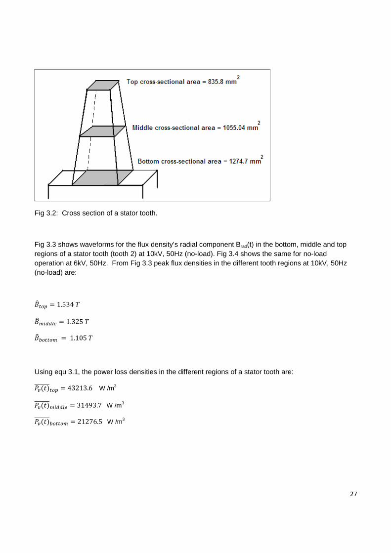
Fig 3.2: Cross section of a stator tooth.
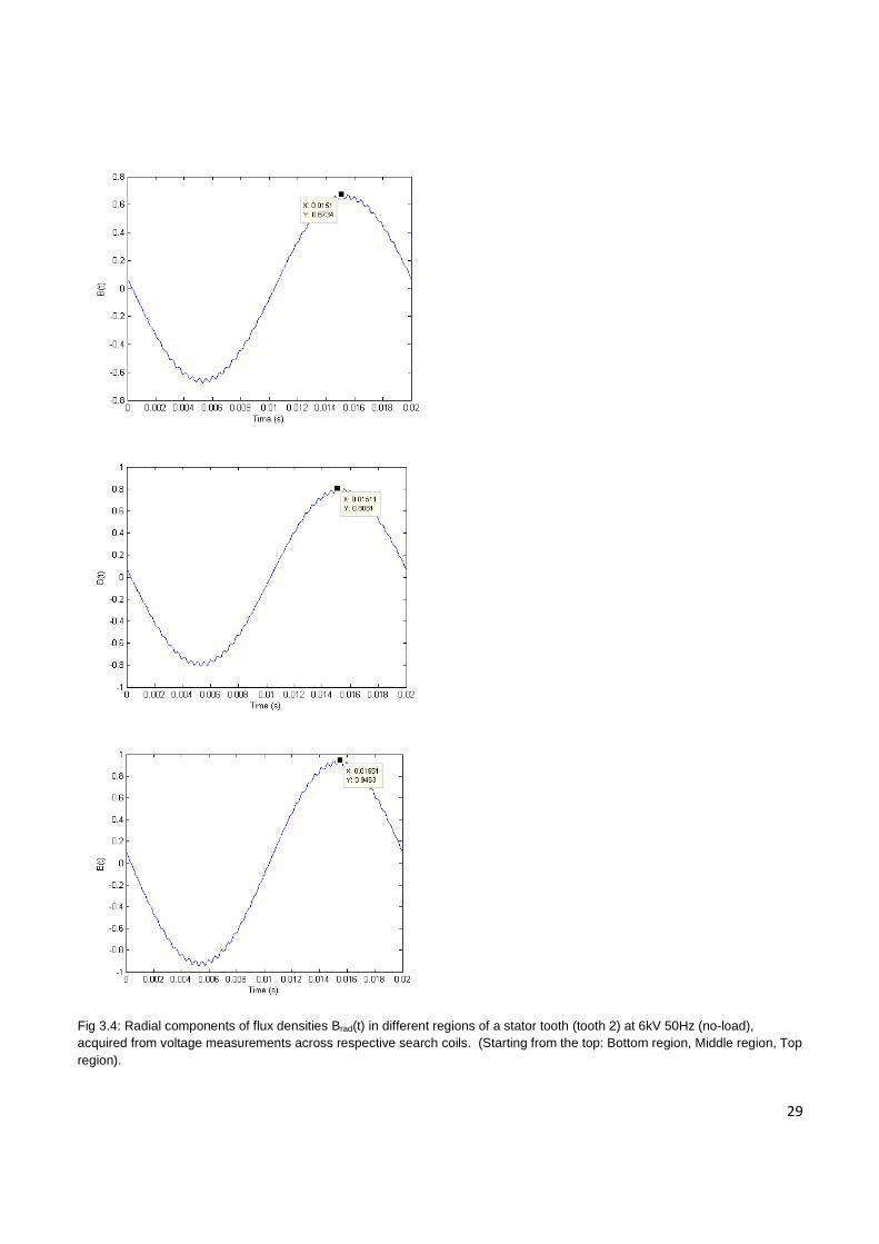
Fig 3.3 shows waveforms for the flux density’s radial component Brad(t) in the bottom, middle and top regions of a stator tooth (tooth 2) at 10kV, 50Hz (no-load). Fig 3.4 shows the same for no-load operation at 6kV, 50Hz. From Fig 3.3 peak flux densities in the different tooth regions at 10kV, 50Hz (no-load) are:
h*| 1.534 >
H$$j 1.325 > *hh*H 1.105 >
Using equ 3.1, the power loss densities in the different regions of a stator tooth are:
h*| 43213.6 W /m3
H$$j 31493.7 W /m3
*hh*H 21276.5 W /m3

28
Fig 3.3: Radial components of flux densities Brad(t) in different regions of a stator tooth (tooth 2) at 10kV 50Hz (no-load), acquired from voltage measurements across respective search coils. (Starting from the top: Bottom region, Middle region, Top region). Plots shown in Fig 3.3 are out of phase since voltage measurements across the bottom, middle and top search coils are with respect to different trigger signals that vary in phase.
29
Fig 3.4: Radial components of flux densities Brad(t) in different regions of a stator tooth (tooth 2) at 6kV 50Hz (no-load), acquired from voltage measurements across respective search coils. (Starting from the top: Bottom region, Middle region, Top region).
30
Equ 3.2 is used to calculate iron loss in the stator teeth.
hhT _*A . h+. TQ . I _*A. h+. T
Q . I _*AQ. h+Q. TQ . . :hhT . :+Th_|i)i+ equ 3.2
It amounts to 8.9 kW for all the stator teeth, assuming all teeth have the same flux density variations as tooth 2.
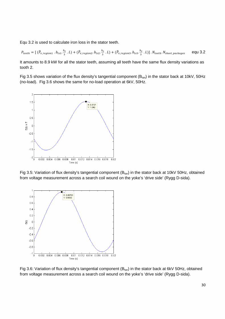
Fig 3.5 shows variation of the flux density’s tangential component (Btan) in the stator back at 10kV, 50Hz (no-load). Fig 3.6 shows the same for no-load operation at 6kV, 50Hz.
Fig 3.5: Variation of flux density’s tangential component (Btan) in the stator back at 10kV 50Hz, obtained from voltage measurement across a search coil wound on the yoke’s ‘drive side’ (Rygg D-sida).
Fig 3.6: Variation of flux density’s tangential component (Btan) in the stator back at 6kV 50Hz, obtained from voltage measurement across a search coil wound on the yoke’s ‘drive side’ (Rygg D-sida).

31
Using equ 3.1 the power loss density in the stator back at 10kV, 50Hz (no-load) is equal to
43702 W/ m3
The total iron loss occurring in the stator back at 10kV, 50Hz (no-load) amounts to 31 kW assuming that the complete yoke behaves as the cross section where the search coil is wound.
Hence, total stator iron losses predicted by the basic Steinmetz equation are:
+hih* 40 at no-load, 50Hz, 10kV for M600-50A.
3.4 Applying the Modified Steinmetz equation (MSE) for iron loss calculation:
In this section stator iron losses predicted by the MSE (equ 3.3 and equ 3.4) are presented. Equ 3.5 relates the RMS search coil voltage to the rate of change of flux density squared.
22 2
0
2( )
T
eq
dBf dt
B dtπ=
∆ ∫ equ 3.3
. . . equ 3.4
899 :. ;. <,1 >? 7 34 50 equ 3.5
The power loss density in each tooth region as well as the stator yoke is calculated using equations 3.3,
3.4 and 3.5. Table 3.1 presents the results.
SEARCH COIL
POSITION
Veff (V) ¡ (T)
feq (Hz) ∆B ¢£ (W/m3)
Tooth bottom 1.5 1.105 71.69 2.21 28385
Tooth middle 1.49 1.325 72.3 2.65 42302
Tooth top 1.4 1.53 71.46 3.07 57504
Stator back 7.3 1.54 51.46 3.08 44720
Table 3.1: Results acquired by applying the MSE to search coil measurements (For M600-50A at 10kV,
50Hz, no-load).

32
Power loss in the stator teeth and yoke were calculated as 11.9 kW and 31.3 kW respectively, using power loss densities presented in table 3.1. Hence, the total stator iron loss predicted by the Modified Steinmetz equation (MSE) at no-load 10kV, 50Hz is 43.2 kW.
For the purpose of comparison, iron losses in the stator teeth and yoke have been calculated using empirical equations (equ 3.6 & 3.7) proposed in [12].
hhT 0.078100 I X/X/% . bh+. 10Q equ 3.6
with bh+ the weight of the stator teeth equal to 1813 kg
h+ 1.105 > (Peak flux density at tooth bottom) (Fig 3.3),
h+ 1.534 > (Peak flux density at tooth top) (Fig 3.3),
50 `¤,
5.17 /¥ (Loss factor at 1.5T and 50 Hz) (From data sheet for M600-50A [16])
It yields
hhT 9.55
+hih* i) 0.078100 I +. b+. 10Q equ 3.7
with b+ the weight of the stator yoke equal to 5419 kg
+ 1.542 > (Peak flux density in stator back) (Fig 3.5),
5.17 /¥ (Loss factor at 1.5T and 50 Hz) (From data sheet of M600-50A [16]),
It yields
+hih* i) 39

33
3.5 Applying the Natural Steinmetz extension (NSE) for iron loss calculation:
In this section stator teeth and stator back iron losses calculated using the NSE (equ 3.8 and equ 3.9) have been presented.
(n^ ∆X
¦§3 ¨$X
$h ¨3
4 5 equ 3.8
( |)*+ | $ %&
' equ 3.9
The power loss density (W/ m3) in each tooth region of a stator tooth (tooth 2) as well as the stator yoke is calculated using equ 3.8. The constant kN has been calculated using equ 3.9 and was found to equal 1.1 for M600-50A. The calculated value of kN is consistent with the plot of (kN / k) versus α given in [5]. Table 3.2 presents the results.
SEARCH COIL
POSITION
¡ (T)
∆B PNSE (W/m3)
Tooth bottom 1.105 2.21 30411
Tooth middle 1.325 2.65 45319
Tooth top 1.534 3.068 61593
Stator back 1.542 3.084 46564
Table 3.2: Results acquired by applying the NSE to search coil measurements (For M600-50A at 10kV, 50Hz, no-load).
Power loss in the stator teeth and yoke were calculated as 12.7 kW and 33 kW respectively using loss densities presented in table 3.2. Hence, the total stator iron loss predicted by the Natural Steinmetz extension (NSE) at no-load 10kV, 50Hz is 45.7 kW.

34
3.6 Comparison of results acquired from different Steinmetz models for M600-50A:
Tables 3.3 and 3.4 present results obtained by applying different iron loss models to search coil measurements acquired at different operating conditions. Model Stator teeth losses Stator back losses Total Stator iron
losses Basic Steinmetz equation
8.9 kW 31 kW 40 kW
MSE 11.9 kW 31.3 kW 43.2 kW NSE 12.7 kW 33 kW 45.7 kW Equations proposed in [12]
9.55 kW 39 kW 49 kW
Table 3.3: Stator iron losses at 50 Hz 10kV during the machine’s heat run test at no-load, obtained by applying different models (For steel grade M600-50A). Looking at table 3.3, the stator iron losses predicted by the MSE are 8% higher in comparison to the value predicted by the basic Steinmetz equation. This is because the MSE takes into account the non-sinusoidal nature of stator teeth flux density waveforms by introducing an equivalent frequency. Equations for iron loss calculation proposed in [12] predict stator iron losses that are 23 % higher as compared to what is predicted by the basic Steinmetz equation. Table 3.4 presents results for the no-load test at 50Hz 6kV. They have been acquired using a similar method, as was adopted for the ‘no-load heat run test’ at 50 Hz 10 kV. The no-load test at 50Hz, 6kV gives roughly 35 % of the stator iron losses at 50Hz, 10kV. Furthermore, the iron losses calculated using empirical equations proposed in [12], were found to estimate 33% higher stator iron losses in comparison to the prediction made by the basic Steinmetz equation.
Model Stator teeth losses Stator back losses Total Stator iron
losses Basic Steinmetz equation
3.1 kW 10.7 kW 13.8 kW
MSE 4.2 kW 10.9 kW 15.1 kW NSE 4.5 kW 11.3 kW 15.8 kW Equations proposed in [12]
3.6 kW 14.8 kW 18.4 kW
Table 3.4: Stator iron losses at 50 Hz 6 kV during the machine’s no-load test, obtained by applying different models (For steel grade M600-50A).

35
3.7 Calculation of stator iron loss for steel grade M400-50A:
Steinmetz parameters (k, α and β) for M400-50A were acquired by curve fitting the basic Steinmetz equation (equ 2.1) to the loss density data available in its data sheet for different frequencies. Fig 3.7 shows the curve fit. They were found to be k=12 , α=1.70 and β=2.61. The value of kN in equ 3.9 for M400-50A was computed as 1. This value is consistent with the plot of (kN / k) versus α in [5]. Tables 3.5 and 3.6 present stator iron losses for steel grade M400-50A at two different operating conditions, namely, no-load operation at 50Hz, 10 kV and no-load operation at 50Hz, 6kV. The presented stator iron losses have been calculated using peak flux densities obtained from search coil measurements.
Model Stator teeth losses Stator back losses Total Stator iron losses
Basic Steinmetz equation
5.5 kW 20.1 kW 25.6 kW
Modified Steinmetz equation (MSE)
7.1 kW 20.5 kW 27.6 kW
Natural Steinmetz extension (NSE)
7.4 kW 20.6 kW 28 kW
Equations proposed in [12]
6.6 kW 26.7 kW 33.3 kW
Table 3.5: Stator iron losses at 50 Hz 10kV during the machine’s heat run test at no-load, obtained by applying different models (For steel grade M400-50A).
Model Stator teeth losses Stator back losses Total Stator iron losses
Basic Steinmetz equation
1.5 kW 5.7 kW 7.2 kW
Modified Steinmetz equation (MSE)
2 kW 5.7 kW 7.7 kW
Natural Steinmetz extension (NSE)
2.1 kW 5.8 kW 7.9 kW
Equations proposed in [12]
2.5 kW 10.2 kW 12.7 kW
Table 3.6: Stator iron losses at 50 Hz 6kV during the machine’s no-load test, obtained by applying different models (For steel grade M400-50A).

36
Fig 3.7: Curve fit for M400-50A at different operating frequencies (For k=12, α=1.70 and β=2.61).
For M400-50A, the MSE predicted 8% and 7% higher stator iron losses than the basic Steinmetz equation at 50Hz, 10kV and 50Hz, 6kV respectively. Percentage increase in iron losses predicted by the empirical equations of [12], in comparison to losses calculated using the basic Steinmetz equation was 30% at 50Hz, 10kV and 76% at 50Hz, 6kV. Furthermore, for M400-50A, the no-load test at 50Hz, 6 kV gives roughly 28% of stator iron losses at 50Hz,10kV.
Comparing the losses of M600-50A and M400-50A, the ratio (PMSE,M600,10kV / PMSE,M400,10kV) is around 1.6, while the ratio (PMSE,M600,6kV / PMSE,M400,6kV) is around 2. Ideally these ratios should equal 1.5. A possible reason for the observed discrepancies is that Steinmetz parameters for M600-50A represent material behavior at 50Hz only, while the ones for M400-50A have been acquired by performing curve fitting over a wide range of frequencies. However, to say anything conclusive in this regard, Steinmetz parameters for M600-50A will have to be acquired for a wide range of frequencies and losses re-calculated.
This chapter presented flux density waveforms for the stator yoke and different regions of a tapered stator tooth, acquired using search coil voltage measurements. Different Steinmetz models were applied to these waveforms. The following chapter applies the loss separation model to the same flux density waveforms presented in this chapter.

37
Chapter 4
Loss separation model applied to search coil measurements on a 15MW induction motor
The aim of this chapter is to present stator iron losses of a 15 MW fractional conductor winding induction motor, calculated using a loss separation approach. The loss separation model classifies iron losses into three types, namely, the hysteresis loss, classical eddy current loss and excess loss (anomalous loss). In this analysis the loss separation model has been applied to determine iron losses occurring during a ‘heat run’ test, with the motor operating at rated voltage (10kV) and rated frequency (50Hz) at no-load. The steel grade chosen for this study is M400-50A [16]. Voltage data across search coils and a portion of the Matlab code used in this analysis, are the outcome of previous work done by Henrik Grop.
4.1 Stator yoke iron loss calculated using a loss separation approach:
4.1.1 Classical eddy current loss in the stator yoke:
The classical eddy current loss per unit volume (Pc) occurring in the stator yoke may be calculated using equ 4.1
) ,6%9M%$%N 0 . ∑ FA A (n is odd) equ 4.1
d = 0.50 mm (Lamination thickness acquired from data sheet of SURA M400-50A)
σ (Conductivity) = 2.38 . 106 Sm-1 (From data sheet of SURA M400-50A)
fm = 50 Hz (Magnetization frequency)
Table 4.1 shows the harmonic amplitudes and phase angles of the flux density waveform in the stator yoke (fig 3.5, chap 3), retrieved by integrating the search coil voltage and dividing by the product of the yoke’s cross sectional area and the number of search coil turns. A Fast Fourier transform (FFT) is applied on the flux density time variations in Matlab.
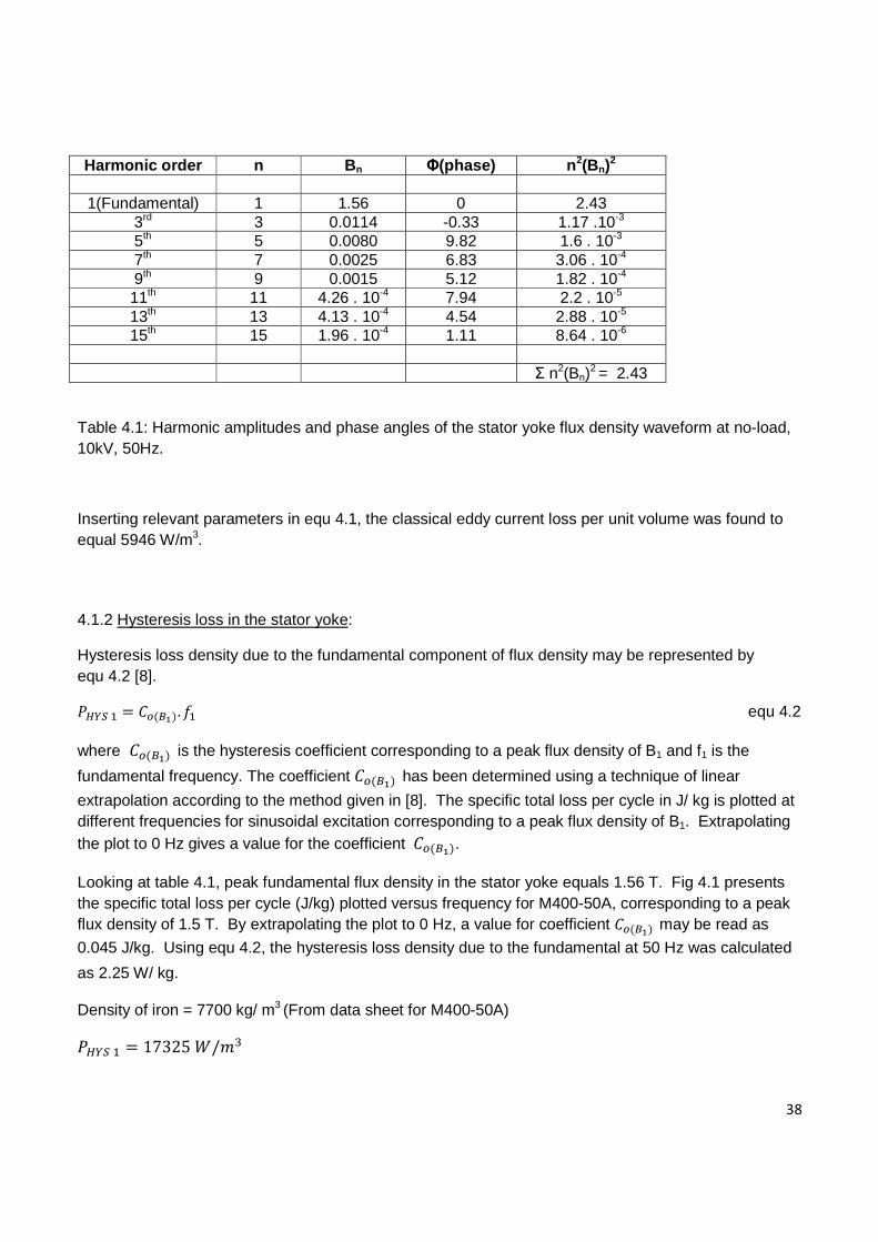
38
Harmonic order n Bn Φ(phase) n2(Bn)2
1(Fundamental) 1 1.56 0 2.43
3rd 3 0.0114 -0.33 1.17 .10-3 5th 5 0.0080 9.82 1.6 . 10-3
7th 7 0.0025 6.83 3.06 . 10-4 9th 9 0.0015 5.12 1.82 . 10-4 11th 11 4.26 . 10-4 7.94 2.2 . 10-5
13th 13 4.13 . 10-4 4.54 2.88 . 10-5
15th 15 1.96 . 10-4 1.11 8.64 . 10-6
Σ n2(Bn)
2 = 2.43
Table 4.1: Harmonic amplitudes and phase angles of the stator yoke flux density waveform at no-load, 10kV, 50Hz.
Inserting relevant parameters in equ 4.1, the classical eddy current loss per unit volume was found to equal 5946 W/m3.
4.1.2 Hysteresis loss in the stator yoke:
Hysteresis loss density due to the fundamental component of flux density may be represented by equ 4.2 [8].
lmn g*X. equ 4.2
where g*X is the hysteresis coefficient corresponding to a peak flux density of B1 and f1 is the
fundamental frequency. The coefficient g*X has been determined using a technique of linear
extrapolation according to the method given in [8]. The specific total loss per cycle in J/ kg is plotted at different frequencies for sinusoidal excitation corresponding to a peak flux density of B1. Extrapolating the plot to 0 Hz gives a value for the coefficient g*X.
Looking at table 4.1, peak fundamental flux density in the stator yoke equals 1.56 T. Fig 4.1 presents the specific total loss per cycle (J/kg) plotted versus frequency for M400-50A, corresponding to a peak flux density of 1.5 T. By extrapolating the plot to 0 Hz, a value for coefficient g*X may be read as
0.045 J/kg. Using equ 4.2, the hysteresis loss density due to the fundamental at 50 Hz was calculated
as 2.25 W/ kg. Density of iron = 7700 kg/ m3 (From data sheet for M400-50A)
lmn 17325 /¬Q

Fig 4.1: Variation of specific total loss per cycle versus frequency for M400
Sources of error in the calculated value of hysteresis loss are as follows:
• The available loss density data is for a peak flux density of 1.5 T. Ideally data corresponding to a peak flux density of 1.6 T should have been used, since the peak fundamental flux densitthe stator yoke is 1.56 T ≈ 1.6 T.
• Hysteresis loss due to harmonics has been disregarded due to nondata corresponding to peak harmonic amplitudes.
: Variation of specific total loss per cycle versus frequency for M400-50A at 1.5T.
error in the calculated value of hysteresis loss are as follows:
The available loss density data is for a peak flux density of 1.5 T. Ideally data corresponding to a peak flux density of 1.6 T should have been used, since the peak fundamental flux densit
≈ 1.6 T.
Hysteresis loss due to harmonics has been disregarded due to non-availability of loss density data corresponding to peak harmonic amplitudes.
39
50A at 1.5T.
The available loss density data is for a peak flux density of 1.5 T. Ideally data corresponding to a peak flux density of 1.6 T should have been used, since the peak fundamental flux density in
availability of loss density

40
4.1.3 Excess loss in the stator yoke:
For sinusoidal excitation, the total loss due to hysteresis, eddy current loss and excess loss is given as:
H TH I v6%9M%$%Xw%N x I 8.67. dab8*;. H |Q/ equ 4.3
In order to determine the product of unknown parameters G and Vo, we need to know the total power loss density P(fm) for a peak sinusoidal induction of Bp as well as the hysteresis loss Ph(fm). The total power loss density at 1.5T and 50 Hz may be read from the datasheet for M400-50A, while the hysteresis loss density was calculated using equ 4.2 in section 4.1.2.
H 27489 /¬Q (Total power loss density at 1.5 T and 50 Hz from datasheet of M400-50A)
TH 17325 /¬Q (Hysteresis loss density corresponding to a peak flux density of 1.5 T at 50 Hz)
Using equ 4.3 the product GVo was calculated as 5.48 .10-5
With GVo known, equ 4.4 was used to compute the power loss density due to excess losses. The integral in equ 4.4 was evaluated in Matlab over one time period.
dab8*; . 1/> |∑ 2FGH AA cos 2FGH I JA|34
Q/ 5 equ 4.4
The power loss density due to excess losses was computed as 4941 W/m3.
4.1.4 Summing together all three components of the loss separation model:
The total power loss density in the stator yoke may be expressed as the sum of classical eddy current, hysteresis and excess loss components.
PT = Ph + Pc + Pe equ 4.5
PT = 28,212 W/m3
Multiplying the total power loss density with the volume of the stator back gives us the iron losses occurring in the stator yoke.
+hih* i) 20
1. S in equ 4.3 and equ 4.4 is the stator back cross-sectional area corresponding to one stator sheet
package. For the particular induction motor being analyzed it equals 5.25 . 10-3 m2

41
4.2 Stator teeth iron losses calculated using a loss separation approach:
To calculate stator teeth iron losses, the stator tooth is divided into three regions (top, center and bottom) as shown in Fig 2.4 and the loss separation model is applied to each region in the same manner as done previously for the yoke.
4.2.1 Classical eddy current loss in the stator teeth:
Table 4.2 presents the classical eddy current loss density in different tooth regions calculated using equ 4.1.
Tooth Region Classical eddy current loss density (Pc) Bottom 2936 W/m3
Center 4199 W/m3
Top 5624 W/m3
Table 4.2: Classical eddy current loss density in different tooth regions (tooth 2).
4.2.2 Hysteresis loss in the stator teeth:
Table 4.3 presents the hysteresis loss coefficients (J/kg) and the hysteresis loss density (W/m3) in the different tooth regions, determined using the technique of linear extrapolation discussed in section 4.1.2. The specific total loss per cycle in J/kg is plotted versus frequency, corresponding to the peak fundamental amplitude of the flux density waveform. Extrapolating this plot to 0Hz, yields a value for the hysteresis loss coefficient.
Tooth Region Hysteresis loss coefficients ® ¯
Hysteresis loss density (Ph) in W/m3
Bottom 0.02 J/ kg 7700 W/m3
Center 0.03 J/kg 11550 W/m3
Top 0.05 J/kg 19250 W/m3
Table 4.3: Hysteresis loss coefficients and hysteresis loss density in different tooth regions (tooth 2).
42
4.2.3 Excess loss in the stator teeth:
Table 4.4 presents the loss density due to excess loss in different tooth regions calculated using equ 4.4.
Tooth Region Loss density due to excess loss (Pe) in W/m3
Bottom 2910 W/m3
Center 3348 W/m3
Top 2815 W/m3
Table 4.4: Loss density due to excess loss in different tooth regions.
4.2.4 Total iron loss in the stator teeth:
Table 4.5 presents the power loss densities in different tooth regions acquired by summing up loss densities due to hysteresis, eddy current and excess losses.
Tooth Region Power Loss Density W/m3
Bottom 13546 W/m3
Center 19097 W/m3
Top 27689 W/m3
Table 4.5: Power loss density in different tooth regions.
Using equ 4.6, the stator teeth loss was calculated as 5.6 kW.
hhT _*A . h+. TQ . I _*A. h+. T
Q . I _*AQ. h+Q. TQ . . :hhT . :+Th_|i)i+ equ 4.6
4.3 Comparison of the Loss separation model with Steinmetz models:
Table 4.6 presents results acquired by applying the loss separation and Steinmetz models. The comparison is done at 10 kV, 50 Hz (no-load), for steel grade M400-50A.
Model Stator yoke loss Stator teeth loss Stator iron loss Loss Separation 20 kW 5.6 kW 25.6 kW
Basic Steinmetz equation 20.1 kW 5.5 kW 25.6 kW MSE 20.5 kW 7.1 kW 27.6 kW NSE 20.6 kW 7.4 kW 28 kW
Table 4.6: A presentation of iron losses predicted by different models at an operating condition of 10kV, 50 Hz (no-load) for steel grade M400-50A.

43
The stator yoke losses predicted by all four models are in close comparison to one another. A percentage difference of roughly 32% exists between stator teeth losses predicted by the Loss Separation model and the Modified and Natural Steinmetz equations (MSE & NSE). This may be attributed to the fact that the MSE and NSE compensate for the non-sinusoidal nature of flux density waveforms in different stator tooth regions. Available data only allows to calculate the loss separation model’s hysteresis component for fundamentals of stator tooth flux density waveforms. Hysteresis loss due to harmonics has been neglected.

44
Chapter 5
Analytical model for calculating stator teeth and yoke flux density variations
The aim of this chapter is to calculate flux densities in the stator teeth and the stator yoke, using analytic models described in [15]. Some of the main assumptions made in the calculations that follow are:
• The stator yoke is excited by an airgap flux density wave.
• The entire airgap flux of one stator slot pitch passes through the corresponding stator tooth.
• Flux is guided in a radial direction through the stator teeth.
5.1 Analytic model for calculating magnetic flux density in a stator tooth:
The airgap flux density wave exciting the stator may be represented as a Fourier series expansion by equ 5.1 [15].
°, ∑ ±k . sin |° ² \ equ 5.1
where
is the amplitude of the vth harmonic.
| G/³| is the fundamental wave number and ³| is the pole pitch in m.
\ 2G is the fundamental angular frequency.
° is the circumferential coordinate.
The flux per length through one stator tooth is given by equ 5.2 [15].
Jh ´ jµjM
. ∑ ¶%
¶%
±k . sinO° ² \ 5° equ 5.2
where
·¸ is the axial airgap length.
·H is the axial magnetic length of the stator.
³+ is the stator slot pitch in m.

45
The magnetic flux density in a stator tooth is given by equ 5.3 [15], assuming it to be equally distributed in the teeth cross sections.
h J ¹ / º . ∑ ±k . . sin ²\ equ 5.3
where
h+ is the tooth width.
º is the tooth area reduction factor given by equ 5.4.
is the harmonic reduction factor given by equ 5.5.
º »/
. jµjM
equ 5.4
!" WO ¶% WO ¶
% equ 5.5
5.2 Calculation of stator tooth flux density using analytic model:
The magnetic flux density in a stator tooth has been calculated analytically for three operating conditions, namely, no-load operation at 10kV 50 Hz , no-load operation at 6kV 50Hz and no-load operation at 10kV 40Hz. Table 5.1 presents harmonic amplitudes of the airgap flux density wave at these three operating conditions, acquired by means of FEM simulations. Apart from the fundamental, only the 35th and 37th harmonics have been included in this analysis, since they were prominent in the frequency spectrum. Fig 5.1 shows the harmonic spectrum of the air gap flux density wave at 10kV, 50Hz (no-load), while Fig 5.2 shows the airgap flux density plotted as a function of the circumferential coordinate ‘x’ in equ 5.1.
Harmonic order 10 kV, 50 Hz, no-load 6 kV, 50 Hz, no-load 10 kV, 40 Hz, no-load 1 (Fundamental) 0.76 T 0.45 T 1.03 T
35 0.15 T 0.09 T 0.23 T 37 0.13 T 0.077 T 0.18 T
Table 5.1: Harmonic amplitudes of the airgap flux density wave at three different operating conditions.

46
Fig 5.1: Frequency spectrum of airgap flux density wave at no-load, 10kV, 50 Hz
Fig 5.2: Airgap flux density wave plotted as a function of the circumferential coordinate at 10kV, 50Hz, no-load.

47
Geometrical parameters for the particular 15 MW induction machine being analyzed are as follows:
³+ 41.9 ¬¬ (Stator slot pitch)
·¸ 1592 ¬¬ (Axial length of airgap)
·H 1344 ¬¬ (Axial magnetic length of the stator core)
h+ 25.12 ¬¬ (Average stator tooth width)
³| 754.2 ¬¬ (Pole pitch)
Vteeth (Total volume of stator teeth in m3) = 0.234 m3
Vstator yoke (Total volume of stator yoke in m3) = 0.7 m3
Using equ 5.4, the tooth area reduction factor º , was calculated as 1.98.
Table 5.2 presents the harmonic reduction factor calculated using equ 5.5, for the fundamental, 35th and 37th harmonics.
Harmonic order Harmonic reduction factor (fv) 1 (Fundamental) 1
35 0.029 37 0.027
Table 5.2: Harmonic reduction factor for different harmonics.
Figures 5.3, 5.4 and 5.5 present the stator tooth flux density calculated using equ 5.3 for three different operating conditions.
Fig 5.3: Mean flux density in a stator tooth calculated analytically for no-load operation at 10kV, 50Hz. (feq calculated using equ 2.2 for the above waveform is 52.4 Hz)

48
Fig 5.4: Mean flux density in a stator tooth calculated analytically for no-load operation at 6 kV, 50Hz. (feq calculated using equ 2.2 for the above waveform is 52.4 Hz)
Fig 5.5: Mean flux density in a stator tooth calculated analytically for no-load operation at 10kV, 40Hz. (feq calculated using equ 2.2 for the above waveform is 42.6 Hz)
A peak flux density of 2 Tesla in the stator tooth at 10kV, 40Hz is unrealistic. The reason being, that the analytic model does not compensate for magnetic saturation.

49
The tooth flux density waveforms presented in Fig 5.3 to Fig 5.5 assume an average stator tooth width of 25.12 mm. To draw a comparison with tooth flux densities in the bottom, middle and top regions acquired using search coil measurements, equ 5.3 was used to calculate the flux density waveform in each tooth region considering its respective tooth width. Table 5.3 presents the results at no-load, 10kV, 50Hz.
Tooth Region Peak flux density (search coil
measurement)
Peak flux density (Analytic)
% increase with search coil value
used as base Bottom 1.105 T 1.24 T 12.2 % Middle 1.325 T 1.5 T 13.2 %
Top 1.534 T 1.89 T 23.2 %
Table 5.3: A presentation of peak flux densities in different stator tooth regions acquired analytically and by search coil measurements at no-load, 10kV, 50Hz.
The analytic model predicts higher peak flux densities in the different tooth regions, in comparison to search coil measurements. This is because it does not compensate for the effect of magnetic saturation.
5.3 Calculation of stator teeth iron loss using analytically determined tooth flux density:
The analytically calculated stator tooth flux density waveforms (fig 5.3 to 5.5) contain harmonics and, hence, it is reasonable to use the modified Steinmetz equation (equ 5.6) for calculating loss density (W/m3). Multiplying the loss density with the total volume of stator teeth in m3, yields the teeth iron loss. In this analysis, the tooth is not sub-divided into the top, center and bottom regions, as was done previously.
. . . equ 5.6
Steinmetz parameters acquired through curve fitting for two different steel grades are as follows:
• k=15, α=1.8 and β=2.16 for M600-50A • k=12, α=1.7 and β=2.61 for M400-50A
Table 5.4 presents the stator teeth iron loss for different steel grades at three different operating conditions.
Steel grade 10kV,50 Hz (no-load) 6kV, 50Hz (no-load) 10kV, 40Hz (no-load)
M600-50A 10.1 kW 3.24 kW 13.1 kW M400-50A 6.5 kW 1.7 kW 10 kW
Table 5.4: Iron loss occurring in the stator teeth calculated analytically.

50
5.4 Analytic model for calculating flux density’s orthogonal components in the stator yoke:
In [15] an analytic model for calculating the x and y components of flux density at any arbitrary point in the stator yoke is described. The model considers the stator yoke as having a rectangular geometry whose points are defined by cartesian coordinates (x,y). Fig 5.6 is a diagrammatic representation of the yoke, where ‘a’ denotes the yoke height.
Fig 5.6: Rectangular geometry of stator yoke.
The x and y components of flux density corresponding to the vth harmonic are given by equ 5.7 and equ 5.8 respectively [15].
¼ °, ½, ² m . S,Oi¾0!"SOi . cosO° ² \ equ 5.7
¾ °, ½, m . !"S,Oi¾0!"SOi . sinO° ² \ equ 5.8
where ¿ is given by equ 5.9 [15].
m jµjM
ooT equ 5.9
D is the stator bore diameter and h is the stator slot depth in m.
The flux distribution in the stator yoke at an arbitrary point denoted by its cartesian coordinates x and y is represented as equ 5.10 [15].
°, ½, ∑ ¼°, ½, ¾°, ½, ±k equ 5.10
51
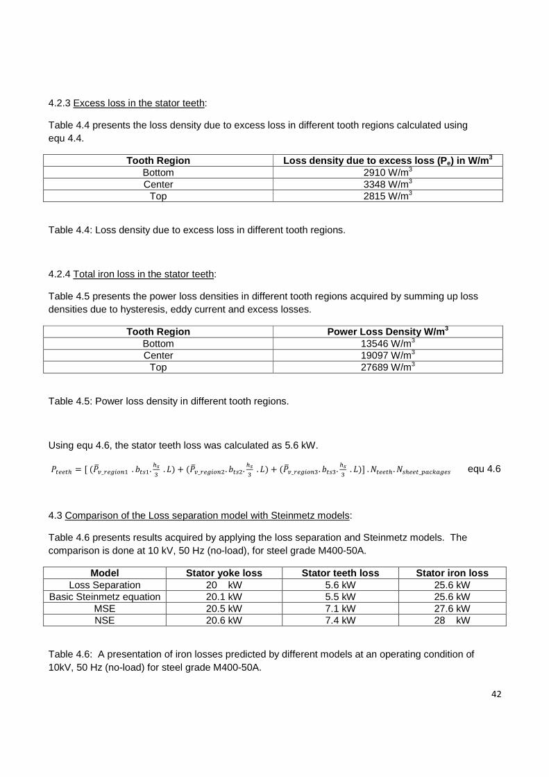
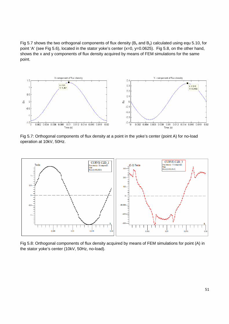
Fig 5.7 shows the two orthogonal components of flux density (Bx and By) calculated using equ 5.10, for point ‘A’ (see Fig 5.6), located in the stator yoke’s center (x=0, y=0.0625). Fig 5.8, on the other hand, shows the x and y components of flux density acquired by means of FEM simulations for the same point.
Fig 5.7: Orthogonal components of flux density at a point in the yoke’s center (point A) for no-load operation at 10kV, 50Hz.
Fig 5.8: Orthogonal components of flux density acquired by means of FEM simulations for point (A) in the stator yoke’s center (10kV, 50Hz, no-load).

52
Table 5.5 presents flux densities and aspect ratios acquired analytically and by means of FEM simulations, at different points along the stator yoke geometry shown in Fig 5.11. The comparison is done for no-load operation at 10kV, 50Hz.
Point Bx (peak) (Analytical)
By (peak) (Analytical)
Aspect Ratio (Analytical)
By / Bx
Btan (peak fundamental)
(FEM)
Brad (peak fundamental)
(FEM)
Aspect Ratio (FEM)
a (0.00625 m) 1.49 T 0.68 T 0.46 1.1 T 0.98 T 0.9 b (0.01875 m) 1.45 T 0.60 T 0.41 1.37 T 0.73 T 0.53 c (0.03125 m) 1.42 T 0.53 T 0.37 1.51 T 0.47 T 0.31 d (0.04375 m) 1.40 T 0.46 T 0.33 1.51 T 0.39 T 0.26 e (0.05625 m) 1.38 T 0.38 T 0.28 1.50 T 0.32 T 0.21 f (0.06875 m) 1.36 T 0.31 T 0.23 1.49 T 0.25 T 0.17 g (0.08125 m) 1.34 T 0.24 T 0.18 1.48 T 0.19 T 0.13 h (0.09375 m) 1.33 T 0.17 T 0.13 1.47 T 0.13 T 0.09 i (0.10625 m) 1.33 T 0.10 T 0.08 1.45 T 0.08 T 0.06 j (0.11875 m) 1.32 T 0.03 T 0.03 1.44 T 0.03 T 0.02
Table 5.5: A presentation of flux densities and aspect ratios acquired analytically and by means of FEM simulations, for different points along the stator yoke geometry (10kV, 50Hz, no-load).
Except for the first point (‘a’) located in the lowest stator yoke volume segment, analytically calculated flux densities and aspect ratios at all other chosen points are in reasonable agreement with corresponding values acquired by FEM simulations. The analytic model gives lower values of Bx in comparison to Btan(FEM) for eight out of ten chosen points, with the percentage difference ranging between 5% to 10%. The analytic model rightly captures the following trends also observed in FEM simulations:
• Flux density’s y-component (radial component) gradually diminishes as distance along the stator yoke’s radial direction increases.
• The aspect ratio of the flux density locus decreases as distance along the yoke’s radial direction increases.

53
Fig 5.9 shows the elliptical flux density locus for point ‘A’ in the yoke’s center (see Fig 5.6).
Fig 5.9: Analytically calculated flux density locus for a point in the yoke’s center (point A) at no-load 10kV, 50Hz (Aspect ratio = 0.35 / 1.37 = 0.25).
The aspect ratio, which is defined as the ratio of the minor axis to the major axis of an elliptical flux density locus, is plotted versus the stator yoke height in Fig 5.10. It can be seen from the figure that as the yoke height increases in the radial direction, the aspect ratio decreases, implying that the magnetic field becomes less rotational and more alternating.
Fig 5.10: Aspect Ratio (Bminor / Bmajor) plotted versus stator yoke height (values from analytic model).

54
5.5 Calculation of stator yoke iron loss using analytically determined yoke flux densities:
In order to calculate iron losses in the stator yoke analytically, the yoke’s rectangular geometry has been divided into ten equal segments as shown in Fig 5.11. For each segment, a point is chosen in its center and the orthogonal components of flux density (Bx & By) at that point are calculated using equ 5.10. Thereafter, individual loss densities (W/m3) due to Bx and By flux density waveforms are determined by applying the Natural Steinmetz Extension (NSE) to each one separately. Multiplying the respective loss densities with the volume of a stator yoke segment (0.07 m3) yields alternating losses along the two orthogonal directions. This model assumes that a point chosen in the center of a stator yoke segment is representative of that entire segment.
Fig 5.11: Stator yoke’s rectangular geometry divided into 10 equal segments.
To calculate rotational losses due to an elliptical field equ 5.11 is used, which multiplies the sum of alternating losses along the two orthogonal directions by a correction factor termed as the loss factor [9] [10]. It should be noted that the loss factor in equ 5.11 is a means of relating rotational losses with the sum of losses produced by orthogonal components of flux density [9]. It does not take into account the fact that magnetic properties are different in directions perpendicular or parallel to the lamination rolling direction.
Z, | f/,Xwf'°Xwf'°Xw equ 5.11
The loss factor ( Z corresponding to a particular aspect ratio ( and peak flux density along major axis
( | is determined using equ 5.12. Factors ] and Z, O O0.1 > in equ 5.12 are directly read from
plots given in [10] for non-oriented samples (see section 2.3).
] Z,XwZ,Xw.w'.
equ 5.12

55
Tables 5.6 and 5.7 present results acquired by applying the described analytic method for steel grade M600-50A at 50Hz, 10kV (no-load).
Point Bx (Bmajor) (peak value)
(Analytic)
By (Bminor) (peak value)
(Analytic)
Aspect RatioÀ (Analytic)
Loss factor ratio (Á
ÂÀ, ÃÄ ÃÄÅ.¯ Æ Loss factor
ÂÀ, ÃÄ
a 1.49 T 0.68 T 0.46 0.78 1.12 0.87 b 1.45 T 0.60 T 0.41 0.83 1.1 0.91 c 1.42 T 0.53 T 0.37 0.85 1.09 0.93 d 1.40 T 0.46 T 0.33 0.87 1.08 0.94 e 1.38 T 0.38 T 0.28 0.90 1.07 0.96 f 1.36 T 0.31 T 0.23 0.93 1.05 0.98 g 1.34 T 0.24 T 0.18 0.95 1.03 0.98 h 1.33 T 0.17 T 0.13 0.97 1.02 0.99 i 1.33 T 0.10 T 0.08 0.98 1.01 0.99 j 1.32 T 0.03 T 0.03 1.0 1.0 1.0
Table 5.6: Bx, By, aspect ratio ( and loss factor for different points in the stator yoke geometry (from analytic model). (M600-50A, 10kV 50Hz No-load).
Stator yoke segments denoted by their respective points
Loss due to Bx
4° | kW Loss due to By
4° | kW
Rotational loss
*h, | kW
a 2.85 0.53 (2.85+0.53) x 0.87 = 2.94 b 2.71 0.41 2.84 c 2.59 0.31 2.70 d 2.49 0.22 2.55 e 2.41 0.15 2.46 f 2.34 0.10 2.39 g 2.28 0.06 2.29 h 2.24 0.03 2.25 i 2.22 0.01 2.21 j 2.21 0.00 2.21 ΣPx = 24.3 ΣPy = 1.82 ΣProt = 24.8
Table 5.7: Losses occurring in each segment of the yoke’s rectangular geometry at no-load 50Hz, 10kV for M600-50A.
The results presented in table 5.7 suggest that rotational losses increase the stator yoke iron loss by 2% in comparison to iron losses produced by the flux density’s tangential component (Bx) alone (ΣPx). For operation at 6kV, 50Hz, this percentage increase above ΣPx was slightly higher and amounted to 8% for M600-50A and 5% for M400-50A.

56
Stator yoke iron losses were calculated using the described method for two steel grades at three different operating conditions. Table 5.8 presents the results.
Steel grade 10kV,50 Hz (no-load) 6kV, 50Hz (no-load) 10kV, 40Hz (no-load) M600-50A 24.8 kW 8.5 kW 31 kW M400-50A 15.2 kW 4.1 kW 22 kW
Table 5.8: Stator yoke iron loss at three different operating conditions.
5.6 Suggested improvement in stator yoke iron losses based on a study of flux distribution in the yoke:
Flux density variation shown in table 5.5 is plotted in Fig 5.12 and Fig 5.13. However, it only represents flux density behavior in the stator yoke along a line aligned with a stator tooth as shown in Fig 5.14. It was observed that the orthogonal components of flux density (Btan and Brad) vary differently in the stator yoke along a line aligned with a stator slot. These plots are shown in figures 5.15 & 5.16. The analytic model only captures variation in the yoke flux density’s orthogonal components along a line aligned with a stator tooth.
Fig 5.12: A comparison of the yoke flux density’s orthogonal components acquired analytically and by FEM simulations at 10kV 50Hz no-load (Only representative of a line in the stator yoke aligned with a tooth).
57
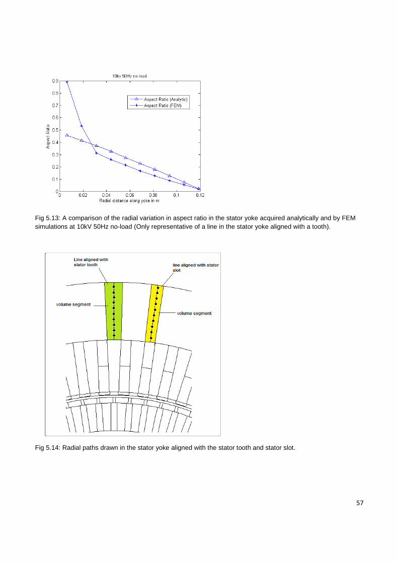
Fig 5.13: A comparison of the radial variation in aspect ratio in the stator yoke acquired analytically and by FEM simulations at 10kV 50Hz no-load (Only representative of a line in the stator yoke aligned with a tooth).
Fig 5.14: Radial paths drawn in the stator yoke aligned with the stator tooth and stator slot.

58
Fig 5.15: Yoke flux density’s orthogonal components acquired by FEM simulations at 10kV 50Hz no-load (Only representative of a radial line in the stator yoke aligned with a slot).
Fig 5.16: Radial variation in aspect ratio in the stator yoke acquired by FEM simulations at 10kV 50Hz no-load (Only representative of a radial line in the stator yoke aligned with a slot).
A new radial variation of flux densities and aspect ratios for yoke volume segments aligned with stator slots should be derived and combined with the existing analytical model to obtain an improved estimate of stator yoke iron loss.

59
Chapter 6
Calculation of iron losses by FEM simulations
This chapter discusses the computation of stator iron losses of a 15 MW fractional conductor winding induction motor by means of post-process of FEM simulations performed in Flux 2D. The Flux geometry file and its associated circuit for no-load simulation used in this analysis, are the outcome of previous work done by Henrik Grop. The Flux 2D iron loss model is based on Bertotti’s formulas [20] [21]. Stator iron losses have been simulated for two steel grades, namely, M600-50A and M400-50A.
6.1 Flux 2D Iron loss model:
The FEM software ‘Flux 2D’ computes iron loss density (W/m3) in each mesh region using equ 6.1 [21] [22].
Ç*A_È^É T¾+h . . 9. I Ê ËÌt.ÍÎÏM²
ÍÑÒÍÒ I kÔÕ ÍÑÒ
ÍÒ Q/ÖÊ4 9 5 equ 6.1
Assuming a sinusoidal flux density variation, the loss density in W/m3 is given by equ 6.2 [21][23].
Ç*A_È^É Ë T¾+h . . I G 6t.$ÎÏM%N . I 8.67 ¼) . u
% Ö . 9 equ 6.2
where
T¾+h is the hysteresis loss coefficient in WsT-2m-3
a*A is the classical losses coefficient in Sm-1
5jiH is the lamination thickness in m
¼) is the excess loss coefficient in W(Ts-1)-3/2m-3
6.2 Determination of Bertotti coefficients for M600-50A:
Bertotti coefficients for the stator yoke and stator teeth regions were defined as follows for steel grade M600-50A:
1. Hysteresis loss coefficient (T¾+h = 210 WsT-2m-3
2. Classical losses coefficient (a*A = 3.33 . 106 Sm-1 (From data sheet for M600-50A) 3. Excess loss coefficient (¼) = 1.2 W(Ts-1)-3/2m-3 4. Lamination thickness (5jiH = 0.5 . 10-3 m 5. Stacking factor = 1 (Assumed) 6. Source frequency (f) = 50 Hz or 40 Hz (Depending on the operating condition)

60
T¾+h and ¼) were acquired by curve fitting equ 6.2 to the loss density data at 50 Hz for M600-50A,
as shown in Fig 6.1. Since the datasheet for M600-50A does not provide loss density data at 40Hz, it is assumed that the acquired values for coefficients T¾+h and ¼) , apply at 40 Hz as well. However, it
is pertinent to mention that the acquired values of T¾+h and ¼) for M600-50A are highly uncertain,
since they represent material behavior at 50Hz only.
Fig 6.1: Power loss densities at different flux densities from Flux 2D iron loss model and data sheet for SURA M600-50A (For T¾+h = 210 WsT-2m-3 and ¼) = 1.2 W(Ts-1)-3/2m-3)
6.3 BH curve for M600-50A:
The BH curve for the steel material defined in Flux 2D matching the data sheet BH curve for M600-50A is shown in Fig 6.2.
Fig 6.2: BH curves for M600-50A at 50 Hz and the steel material defined in Flux 2D.

61
6.4 FEM Simulation results for steel grade M600-50A:
The motor geometry shown in Fig 6.3 was simulated for three different operating conditions. In the post-process, Bertotti coefficients from section 6.2 were applied. Table 6.2 summarizes the iron loss results for steel grade M600-50A.
Fig 6.3: Motor geometry of a fractional conductor winding induction machine.
Table 6.1 presents the peak fundamental flux densities in different tooth regions acquired through search coil measurements and by means of FEM simulation at no-load, 10kV, 50Hz.
Tooth Region Search coil (peak fundamental value)
FEM (peak fundamental of radial component)
% difference with search coil value
as base Bottom 1.085 T 1.13 T 4.1 % Middle 1.303 T 1.30 T 0.23 %
Top 1.51 T 1.56 T 3.3 %
Table 6.1: A presentation of peak fundamental flux densities in different tooth regions acquired through search coil measurements and FEM simulation for M600-50A at no-load, 10kV, 50Hz.
For the yoke flux density waveform acquired using search coil measurements, the peak fundamental flux density is 1.56 T at no-load, 10kV, 50Hz (see table 4.1). For a point taken in the yoke’s center, FEM simulation gave a value of 1.523 T for the peak fundamental of flux density’s tangential component, with M600-50A as the steel grade. The percentage difference between the two values is 2.4 %.

62
6.5 Iron loss for steel grade M600-50A:
Operating condition
Stator yoke loss
(mean value)
Stator teeth loss (mean value)
Total Stator loss
10 kV, 50Hz, no-load
29.6 kW 12.4 kW 42 kW
6 kV, 50Hz, no-load
8.1 kW 3.8 kW 11.9 kW
10 kV, 40Hz, no-load
34.5 kW 12.6 kW 47.1 kW
Table 6.2: Results for steel grade M600-50A from Flux 2D simulations.
The simulated stator iron losses are for the stator core’s axial magnetic length (1344 mm) and the Flux 2D circuit uses current sources to excite each stator phase. At 10kV, 50Hz (no-load) and 6kV, 50Hz (no-load), the rms phase currents are 143.7A and 73.5A respectively. At 10kV, 40Hz (no-load) it is 289A. These values correspond to current measurements acquired from the prototype 15MW induction machine at different no-load operating conditions.
6.6 Iron loss for steel grade M400-50A:
Table 6.3 presents the peak fundamental flux densities in different tooth regions acquired through search coil measurements and by means of FEM simulation at no-load, 10kV, 50Hz, for steel grade M400-50A.
Tooth Region Search coil (peak fundamental value)
FEM (peak fundamental of radial component)
% difference with search coil value
as base Bottom 1.085 T 1.102 T 1.6 % Middle 1.303 T 1.27 T 2.5 %
Top 1.51 T 1.52 T 0.7 %
Table 6.3: A presentation of peak fundamental flux densities in different tooth regions acquired through search coil measurements and FEM simulation for M400-50A at no-load, 10kV, 50Hz.
For the yoke flux density waveform acquired using search coil measurements, the peak fundamental flux density is 1.56 T at no-load, 10kV, 50Hz. For a point taken in the yoke’s center, FEM simulation gave a value of 1.5 T for the peak fundamental of flux density’s tangential component, with M400-50A as the steel grade. The percentage difference between the two values is 3.8 %.

63
The following Bertotti coefficients were defined for steel grade M400-50A and it was ensured that the BH curve for the steel material defined in the FEM software, matched the data sheet BH curve for M400-50A. Fig 6.4 shows the curve fit for the hysteresis and excess loss coefficients at different frequencies.
1. Hysteresis loss coefficient (T¾+h = 170 WsT-2m-3
2. Classical losses coefficient (a*A = 2.38 . 106 Sm-1 (From data sheet for M400-50A) 3. Excess loss coefficient (¼) = 0.65 W(Ts-1)-3/2m-3 4. Lamination thickness (5jiH = 0.5 . 10-3 m 5. Stacking factor = 1 (Assumed) 6. Source frequency (f) = 50 Hz, 40 Hz (Depending on the operating condition)
Table 6.4 summarizes the results for steel grade M400-50A.
Operating condition
Stator yoke loss
(mean value)
Stator teeth loss (mean value)
Total Stator loss
10 kV, 50Hz, no-load
20.8 kW 8.4 kW 29.2 kW
6 kV, 50Hz, no-load
5.9 kW 2.7 kW 8.6 kW
10 kV, 40Hz, no-load
23.1 kW 8.3 kW 31.4 kW
Table 6.4: Results for steel grade M400-50A from Flux 2D simulations.

64
Fig 6.4: Curve fit for M400-50A to acquire khyst and kexc.
(For khyst = 170 WsT-2m-3 and kexc = 0.65 W(Ts-1)-3/2m-3)
Looking at the iron loss results for M400-50A presented in table 6.4, it can be said that the no-load simulation at 50Hz, 6kV gives roughly 29% of stator iron losses at no-load, 50Hz, 10kV. Moreover, for no-load operation at 40Hz, 10kV there is a percentage increase of roughly 8% in stator iron losses, in comparison to iron loss results acquired for no-load operation at 50Hz, 10kV. This increase is attributable to a higher phase current being drawn by the machine at no-load, 40Hz, 10kV, in comparison to the phase current it draws at 50Hz, 10kV.

65
Chapter 7
Conclusions and future work
7.1 Conclusions:
The iron loss study led to the following findings. Iron loss results for no-load operation at 10kV, 50Hz and 6kV, 50Hz have been compiled in table 7.1.
• Equations for iron loss calculation proposed in [12] were found to consistently predict higher
yoke losses at 50Hz in comparison to prediction of yoke losses made by the Steinmetz and loss separation models.
• Iron loss results confirm that the basic Steinmetz equation is only well suited to sinusoidal flux density waveforms and its accuracy diminishes as the flux density waveform becomes increasingly non-sinusoidal. Observe that the percentage difference in losses predicted by the basic Steinmetz equation, as opposed to its modified versions (MSE & NSE) is less for stator yoke losses than for stator teeth losses. This is because the yoke flux density waveform acquired by means of search coil measurements is more sinusoidal in nature than teeth flux density waveforms acquired through a similar method. It may be said that it is more convenient to apply the basic Steinmetz equation to the stator yoke flux density waveform. Applying modified versions of the Steinmetz equation (MSE & NSE) to this waveform results in an increase of less than 10% in yoke iron losses. However, it is recommended to apply the Steinmetz equation’s modified versions to stator tooth flux density waveforms, which exhibit a greater degree of non-sinusoidal character. Applying the basic Steinmetz equation to tooth flux density waveforms, results in an under-estimation of teeth losses by approximately 30%.
• It was verified through FEM simulations that for this particular 15 MW induction machine, the aspect ratio of flux density loci decreases as radial height along the yoke increases, implying that the magnetic field becomes less rotational and more alternating in that direction. The magnetic field is most rotational in the roots of stator teeth. However, results presented in chapter 5 show that rotational fields have a small effect on stator yoke iron loss. The percentage increase above iron losses produced by the flux density’s tangential component alone was found to remain under 10% for all investigated cases. According to [9], their influence is more significant in the rotor.
66
• It may be said that the Steinmetz models are simpler to implement in terms of computational complexity, whereas the loss separation model allows us to compare the relative magnitudes of hysteresis, eddy current and excess losses. The reliability of Steinmetz models is greatly reduced if Steinmetz parameters represent material behavior at the fundamental frequency only. Provided loss density data is available for a wide range of frequencies, it is recommended to acquire a curve fit considering all frequencies. The same applies for the hysteresis and excess loss coefficients appearing in the Flux 2D iron loss model. The technique of linear extrapolation for calculating the hysteresis coefficient in the loss separation model is prone to error due to the following reasons:
At times loss density data at different frequencies, corresponding to the precise peak fundamental amplitude of the flux density waveform is not available, and one has to round off the waveform’s peak fundamental value to the nearest flux density available in the material datasheet.
Hysteresis loss due to harmonics had to be neglected due to non-availability of loss density data corresponding to peak harmonic amplitudes.
• The analytic model for stator yoke iron loss calculation, discussed in chapter 5, is not to be
relied upon for the accuracy of its results. A potential source of error is the fact that analytic equations presented in chapter 5 have their limitations when it comes to accurately predicting the yoke’s flux density map. Furthermore, yoke iron loss results from the analytic model, assume a perfect elliptical flux density locus. Considering the finite elements of a meshed motor geometry, this is often not the case [9]. In this work, the analytic model for stator iron loss calculation has only been used as a tool to determine the contribution made by rotational fields to stator iron losses. It can be concluded that the effect of rotational fields in the stator is highly localized and has a small effect on stator iron losses.

67
7.2 Future work:
Having accurate knowledge of variation in flux density’s orthogonal components in the stator yoke is a pre-requisite for obtaining a good estimate of yoke iron losses. The analytic model discussed in chapter 5 serves as a good starting point, but has its limitations when it comes to accurately capturing flux density behavior in the yoke. There exists a possibility to further improve this analytic model to include the circumferential variation in yoke flux density’s orthogonal components along a slot pitch.
The rotational iron loss model discussed in chapters 2 & 5 does not model the fact that magnetic properties of a steel lamination are different along the two orthogonal directions .i.e. the rolling direction and the direction perpendicular to the rolling direction. The loss factor it introduces is simply a correction factor based on experimental results, which is multiplied by the sum of losses produced by individual orthogonal components, to obtain a better estimate of rotational loss [9] [10]. In future, it would be interesting to use this model coupled with the steel grade’s percentage anisotropy [16][24], to cater for the variation in magnetic properties along the two orthogonal directions.
Furthermore, this study is limited to the machine’s stator. It can be extended to include rotor iron losses, to get a complete picture of the motor’s iron loss at different operating conditions.

68
IRON LOSS MODELS APPLIED TO SEARCH COIL MEASUREMENTS
All Losses are in
kW 50 Hz, 10kV, NO-LOAD 50 Hz, 6kV, NO-LOAD
M600-50A M400-50A M600-50A M400-50A
Stator
teeth
Stator
yoke
Total
stator
Stator
teeth
Stator
yoke
Total
stator
Stator
teeth
Stator
yoke
Total
stator
Stator
teeth
Stator
yoke
Total
stator
BASIC STEINMETZ
EQUATION 8.9 31 40 5.5 20.1 25.6 3.1 10.7 13.8 1.5 5.7 7.2
MSE 11.9 31.3 43.2 7.1 20.5 27.6 4.2 10.9 15.1 2.0 5.7 7.7
NSE 12.7 33 45.7 7.4 20.6 28 4.5 11.3 15.8 2.1 5.8 7.9
LOSS SEPARATION
MODEL / / / 5.6 20 25.6 / / / 2.5 7.8 10.3
EQUATIONS
PROPOSED IN [12] 9.6 39 49 6.6 26.7 33.3 3.6 14.8 18.4 2.5 10.2 12.7
RESULTS FROM FLUX 2D IRON LOSS MODEL (FEM ANALYSIS)
50 Hz, 10kV, NO-LOAD 50 Hz, 6kV, NO-LOAD
M600-50A M400-50A M600-50A M400-50A
Stator
teeth
Stator
yoke
Total
stator
Stator
teeth
Stator
yoke
Total
stator
Stator
teeth
Stator
yoke
Total
stator
Stator
teeth
Stator
yoke
Total
stator
12.4 29.6 42 8.4 20.8 29.2 3.8 8.1 11.9 2.7 5.9 8.6
STEINMETZ IRON LOSS MODEL APPLIED TO ANALYTIC FLUX DENSITY VARIATIONS
50 Hz, 10kV, NO-LOAD 50 Hz, 6kV, NO-LOAD
M600-50A M400-50A M600-50A M400-50A
Stator
teeth
Stator
yoke
Total
stator
Stator
teeth
Stator
yoke
Total
stator
Stator
teeth
Stator
yoke
Total
stator
Stator
teeth
Stator
yoke
Total
stator
10.1 24.8 35 6.5 15.2 22 3.24 8.5 11.7 1.7 4.1 5.8
Table 7.1: A compilation of iron loss results for no-load operation at 10kV, 50Hz and 6kV, 50Hz.

References
[1] C.Steinmetz, “On the law of hysteresis (originally published in 1892),” Proceedings of IEEE, vol 72, no.2, pp. 197-221, 1984.
[2] K. Venkatachalam, C. Sullivan, T. Abdallah and H.Tacca, “Accurate prediction of ferrite core loss with non-sinusoidal waveforms using only Steinmetz parameters,” in IEEE Workshop on Computers in Power Electronics, 2002, pp. 36-41.
[3] A. Krings, J. Soulard, “Overview and comparison of iron loss models for electrical machines,” Journal of Electrical Engineering, vol 10, pg 162-169, Sep 2010.
[4] Jieli Li, T.Abdallah, C.R.Sullivan, “ Improved calculation of core loss with non-sinusoidal waveforms,” in IAS Annual Meeting Conference Records, vol 4, 2001, pp. 2203-2210.
[5] A. Van den Bossche, V.C. Valchev, “ Measurement and loss model of ferrites with non-sinusoidal waveforms,” 35th Annual IEEE Power Electronics Specialists Conference, Aachen Germany, 2004.
[6] F. Fiorillo and A. Novikov, “ An improved approach to power losses in magnetic laminations under non-sinusoidal induction waveform,”IEEE Transactions on Magnetics, vol.24, no.1, pp.621-630, 1988.
[7] G. Bertotti, “Physical interpretation of eddy current losses in ferromagnetic materials.i. theoretical considerations,” J. Appl. Physics, vol 57, no.6, pp.2110-2117, 1985.
[8] J. Leicht, A.J. Moses, S.Zurek, “Hysteresis loss component under non-sinusoidal flux waveforms,” Journal of Magnetism and Magnetic Materials, 320 (2008) p608-p610.
[9] Carlos A. Hernandez-Aramburo, Tim C.Green, Alexander C.Smith, “Estimating rotational iron losses in an induction machine,” IEEE Transactions on Magnetics, vol.39, no.6, Nov 2003.
[10] T. Kochmann, “Relationship between rotational and alternating losses in electrical steel sheets,” Journal of Magnetism and Magnetic Materials, 160 (1996) 145-146.
[11] V.Jaiswal, M.Fazil, A. Hangal and N.Ravi, “Accurate performance prediction of three-phase induction motor by FEM using separate saturation curves for teeth and yoke,” International conference on Power Electronics, Drives and Energy Systems, 2006, DOI:10.1109/PEDES.2006.344346.
[12] C. Sadarangani, Design and analysis of induction and permanent magnet motors, Division of Electrical Machines and Power Electronics, Royal Institute of Technology, Stockholm, 2006.
[13] R. Richter , “Elektrische Maschinen Band IV”, Verlag Birkhäuser, Basel 1954.
[14] H. L. Schenk and F. J. Young, “Iron losses in induction motor teeth,” IEEE Transactions on Magnetics, Vol.17, No.6, Nov 1981.
70
[15] G.Traxler - Samek, G.Ardley, “Iron losses in salient pole synchronous machines considering unidirectional and elliptic magnetization”, CD-ROM Proceedings Electromotion 2009 – EPE Chapter ‘Electric Drives’ Joint Symposium, Lille, France,1-3 July 2009.
[16] Surahammars bruk, company website. http://www.sura.se/
[17] H. Grop, “Investigation of AC Electrical Machine Stators with Fractional Conductor Windings”, Licentiate Thesis, Division of Electrical Machines and Power Electronics, Royal Institute of Technology, Stockholm, Sweden 2010, ISBN:978-91-7415-602-7.
[18] H. Grop, J. Soulard and H. Persson, “Theoretical Investigation of Fractional Conductor Windings for AC-Machines – Definition, Air-gap m.m.f. and Winding Factors”. Proceedings of the 2008 International Conference on Electrical Machines, paper ID 1117.
[19] A. Tessarolo, M. Mezzarobba and A. Contin, “A Stator Winding Design with Unequally-Sized Coils for Adjusting Air-Gap Space Harmonic Content of Induction Machines”, XIX International Conference on Electrical Machines-ICEM 2010, Rome.
[20] Cedrat, User’s guide online help.
[21] A .Stening, “Design and optimization of a surface-mounted permanent magnet synchronous motor for a high cycle industrial cutter”,M.Sc thesis, KTH, 2006.
[22] F. Libert, “Design, Optimization and Comparison of Permanent Magnet Motors for a Low-Speed Direct-Driven Mixer”, Licentiate Thesis, Division of Electrical Machines and Power Electronics KTH, ISBN 91-7283-901-5, Stockholm, 2004.
[23] S.Meier, “Theoretical design of surface-mounted permanent magnet motors with field weakening capability”, Master Thesis, Division of Electrical Machines and Power Electronics KTH, Stockholm, 2002.
[24] T. Ryckebusch, “On uncertainty of lamination properties used in electrical machines”, Master Thesis, Division of Electrical Machines and Power Electronics, Royal Institute of Technology, Stockholm, 2005.

71
List of Symbols
SYMBOL
QUANTITY
UNIT
k Numerical constant in the Steinmetz equation.
-
α
Numerical constant in the Steinmetz equation.
- β
Numerical constant in the Steinmetz equation.
-
Time average power loss per unit volume.
W/m3
eqf Equivalent frequency Hz
∆B
Peak to peak amplitude of the flux density waveform.
T
rf Magnetization frequency Hz fm Magnetization frequency Hz kN Numerical constant in the
Natural Steinmetz extension. -
T Time period of the flux density waveform.
s
d Lamination thickness m 2 Material density kg/ m3 ρ specific resistivity of the material Ωm σ Conductivity of the material Sm-1
Veff Induced RMS voltage across a search coil
V
N Number of search coil turns - S Cross-sectional area m2
Bn nth harmonic amplitude of the flux density waveform
T
g*Xt Hysteresis coefficient corresponding to a peak flux density of Bn
J/ kg
Bp Peak flux density T
2, | Loss factor corresponding to a particular aspect ratio and peak flux density along major axis.
-
Aspect ratio equal to Bminor / Bmajor
-
| Peak flux density along major axis.
T
] Loss factor ratio -
W Loss factor at 1.5 T W/kg
f Electrical frequency Hz

72
SYMBOL QUANTITY UNIT
h+ Peak induction at tooth top. T
h+ Peak induction at tooth bottom. T
bh+ Weight of the stator teeth. kg
+ Peak flux density in the stator back.
T
b+ Weight of the stator yoke kg
Amplitude of the vth harmonic of the exciting air gap flux density wave
T
\ Angular frequency rad/ s
° Circumferential coordinate m
³+ Stator slot pitch m
³| Pole pitch m
h+ Stator tooth width m
hs Stator tooth height m
º Tooth area reduction factor -
Harmonic reduction factor -
D Stator bore diameter m
h Stator slot depth m
a Stator yoke’s radial height m
T¾+h Hysteresis loss coefficient WsT-2m-3
a*A Material conductivity Sm-1
5jiH Lamination thickness m
¼) Excess loss coefficient W(Ts-1)-3/2 m-3

73
List of Figures 2.1A Plot of loss factor ratio (ξ) versus Bminor 2.1B Plot of loss factor (γ) versus aspect ratio for different peak flux densities. 2.2 Flux distribution in a 4 pole induction machine. 2.3 Stator yoke comprising of stator sheet packages. 2.4 Stator tooth divided into three regions, with a search coil wound around each region. 3.1 Power loss densities for different flux densities from basic Steinmetz equation and data sheet for SURA M600-50A (curve fit at 50Hz). 3.2 Cross section of a stator tooth. 3.3 Radial components of flux densities Brad(t) in different regions of a stator tooth at no-load, 10kV, 50Hz. 3.4 Radial components of flux densities Brad(t) in different regions of a stator tooth at no-load, 6kV, 50Hz. 3.5 Variation of flux density’s tangential component (Btan) in the stator back at no-load, 10kV, 50Hz. 3.6 Variation of flux density’s tangential component (Btan) in the stator back at no-load, 6kV, 50Hz. 3.7 Curve fit for M400-50A at different operating frequencies. 4.1 Variation of specific total loss per cycle versus frequency for M400-50A at 1.5T 5.1 Frequency spectrum of the airgap flux density wave at no-load 10kV, 50Hz. 5.2 Airgap flux density wave plotted as a function of the circumferential coordinate at no-load, 10kV, 50Hz. 5.3 Mean flux density in a stator tooth calculated analytically for no-load operation at 10kV, 50Hz. 5.4 Mean flux density in a stator tooth calculated analytically for no-load operation at 6kV, 50Hz. 5.5 Mean flux density in a stator tooth calculated analytically for no-load operation at 10kV, 40Hz. 5.6 Rectangular geometry of the stator yoke. 5.7 Orthogonal components of flux density at a point in the yoke’s center for no-load operation at 10kV, 50Hz. 5.8 Orthogonal components of flux density acquired by means of FEM simulations for point (A) in the stator yoke’s center for no-load operation at 10kV, 50Hz. 5.9 Analytically calculated flux density locus for a point in the yoke’s center (point A) at no-load 10kV, 50Hz. 5.10 Aspect ratio (Bminor /Bmajor) plotted versus stator yoke height (analytic model). 5.11 Stator yoke’s rectangular geometry divided into 10 equal segments. 5.12 A comparison of the yoke flux density’s orthogonal components acquired analytically and by FEM simulations at no-load, 10kV, 50Hz. 5.13 A comparison of the radial variation in aspect ratio in the stator yoke acquired analytically and by FEM simulations at no-load, 10kV, 50Hz. 5.14 Radial paths drawn in the stator yoke aligned with the stator tooth and stator slot. 5.15 Yoke flux density’s orthogonal components acquired by FEM simulations at no-load, 10kV, 50Hz. (Only representative of a radial line in the yoke aligned with a slot). 5.16 Radial variation in aspect ratio in the stator yoke acquired by FEM simulations at no-load, 10kV, 50Hz (Only representative of a radial line in the yoke aligned with a slot). 6.1 Power loss densities at different flux densities from Flux 2D iron loss model and data sheet for SURA M600-50A. 6.2 BH curves for M600-50A at 50Hz and steel material defined in Flux 2D. 6.3 Motor geometry of a fractional conductor winding induction machine. 6.4 Curve fit for M400-50A to acquire khyst and kexc.
74
List of Tables 3.1 Results acquired by applying the MSE to search coil measurements (For M600-50A at 10kV, 50Hz, no-load). 3.2 Results acquired by applying the NSE to search coil measurements (For M600-50A at 10kV, 50Hz, no-load). 3.3 Stator iron losses at 50 Hz 10kV during the machine’s heat run test at no-load, obtained by applying different models (For steel grade M600-50A). 3.4 Stator iron losses at 50 Hz 6kV during the machine’s no-load test, obtained by applying different models (For steel grade M600-50A). 3.5 Stator iron losses at 50 Hz 10kV during the machine’s heat run test at no-load, obtained by applying different models (For steel grade M400-50A). 3.6 Stator iron losses at 50 Hz 6kV during the machine’s no-load test, obtained by applying different models (For steel grade M400-50A). 4.1 Harmonic amplitudes and phase angles of the stator yoke flux density waveform at no-load, 10kV, 50Hz. 4.2 Classical eddy current loss density in different tooth regions (tooth 2). 4.3 Hysteresis loss coefficients and hysteresis loss density in different tooth regions (tooth 2). 4.4 Loss density due to excess loss in different tooth regions. 4.5 Power loss density in different tooth regions. 4.6 A presentation of iron losses predicted by different models at an operating condition of 10kV, 50 Hz (no-load) for steel grade M400-50A. 5.1 Harmonic amplitudes of the airgap flux density wave at three different operating conditions. 5.2 Harmonic reduction factor for different harmonics. 5.3 A presentation of peak flux densities in different stator tooth regions acquired analytically and by search coil measurements at no-load, 10kV, 50Hz. 5.4 Iron loss occurring in the stator teeth calculated analytically. 5.5 A presentation of flux densities and aspect ratios acquired analytically and by means of FEM simulations, for different points along the stator yoke geometry (10kV, 50Hz, no-load). 5.6 Bx, By, aspect ratio ( and loss factor for different points in the stator yoke geometry. (from analytic model), (M600-50A,10kV 50Hz No-load). 5.7 Losses occurring in each segment of the yoke’s rectangular geometry at no-load 50Hz, 10kV for M600-50A. 5.8 Stator yoke iron loss at three different operating conditions. 6.1 A presentation of peak fundamental flux densities in different tooth regions acquired through search coil measurements and FEM simulation for M600-50A at no-load, 10kV, 50Hz. 6.2 Results for steel grade M600-50A from Flux 2D simulations. 6.3 A presentation of peak fundamental flux densities in different tooth regions acquired through search coil measurements and FEM simulation for M400-50A at no-load, 10kV, 50Hz. 6.4 Results for steel grade M400-50A from Flux 2D simulations. 7.1 A compilation of iron loss results for no-load operation at 10kV, 50Hz and 6kV, 50Hz.

75
Appendix
A. Figures complementing Chapter 5: Exciting airgap wave as a function of circumferential coordinate (x in m) at a given time instant:
Fig A.1: Airgap flux density wave at no-load 6kV, 50Hz.
Fig A.2: Airgap flux density wave at no-load 10kV, 40Hz.

76
Frequency spectrum of airgap flux density wave at different operating conditions:
Fig A.3: Frequency spectrum of airgap flux density wave at no-load, 6kV, 50Hz
Fig A.4: Frequency spectrum of airgap flux density wave at no-load, 10kV, 40Hz

77
Comparison of analytic model with FEM simulations at 6kV, 50Hz, no-load:
Fig A.5: A comparison of the yoke flux density’s orthogonal components acquired analytically and by FEM simulations at 6kV 50Hz no-load (Only representative of a line in the stator yoke aligned with a tooth).
Fig A.6: A comparison of the radial variation in aspect ratio in the stator yoke acquired analytically and by FEM simulations at 6kV 50Hz no-load (Only representative of a line in the stator yoke aligned with a tooth).

78
Fig A.7: Yoke flux density’s orthogonal components acquired by FEM simulations at 6kV 50Hz no-load (Only representative of a line in the stator yoke aligned with a slot).
Fig A.8: Radial variation in aspect ratio in the stator yoke acquired by FEM simulations at 6kV 50Hz no-load (Only representative of a line in the stator yoke aligned with a slot).