internet traffic engineering by optimizing ospf weights - infocom

Internet Traffic Engineering by Optimizing OSPF Weights

Bernard Fortz Mikkel Thorup Service de MathCmatiques de la Gestion

Institut de Statistique et de Recherche Op6rationnelle UniversitC Libre de Bruxelles

[email protected] [email protected]

AT&T Labs-Research Shannon Laboratory

Florham Park, NJ 07932 Brussels, Belgium USA

Abstract-Open Shortest Path First (OSPF) is the most commonly used intra-domain internet routing protocol. ’Raffic flow is routed along shortest paths, splitting flow at nodes where several outgoing links are on shortest paths to the destination. The weights of the links, and thereby the shortest patb routes, can be changed by the network operator. The weights could be set proportional to their physical distances, but often the main goal is to avoid congestion, i.e. overloading of links, and the standard heuristic recommended by Cwo is to make the weight of a link inversely proportional to its capacity.

Our startiug point was a proposed AT&T WorIdNet backbone with demands projected from previous measurements. The desire was to optimize the weight setting based on the projected demands. We showed that opti- m i z i i the weight settings for a given set of demands is NP-hard, so we resorted to a local search heuristic. Surprisingly it turned out that for the proposed AT&T WorlWet backbone, we found weight settings that performed within a few percent from that of the optimal general routing where the Bow for each demand is optimally distributed over all paths between source and destination. This contrasts the common belief that OSPF routing leads to congestion and it shows that for the network and demand matrix studied we cannot get a substantially better load balancing by switching to the proposed more flexible Multi-protocol Label Switching (MPLS) technologies. Our techniques were also tested on synthetic internetworks, based on a

model of Zegura et al. (INFOCOM’96), for which we did not always get quite as close to the optimal general routing. However, we compared with standard heuristics, such as weights inversely proportional to the capacity or proportional to the physical distances, and found that, for the same network and capacities, we could support a 50%-110% increase in the demands. Our assumed demand matrix can also be seen as modeling service level

agreements (SLAs) with customers, with demands representing guarantees of throughput for virtual leased lines.

Keywords-OSPF, MPLS, traffic engineering, local search, hashing tables, dynamic shortest paths, multi-commodity network Rows.

I. INTRODUCTION ROVISIONING an Internet Service Provider (ISP) back- P bone network for intra-domain IP traffic is a big challenge,

particularly due to rapid growth of the network and user demands. At times, the network topology and capacity may seem insufficient to meet the current demands. At the same time, there is mounting pressure for ISPs to provide Quality of Ser- vice (QoS) in terms of Service Level Agreements (SLAs) with customers, with loose guarantees on delay, loss, and throughput. All of these issues point to the importance of tr@c engineering, making more efficient use of existing network resources by tai- loring routes to the prevailing traffic.

A. The general routing problem The getzeral routing problem is defined as follows. Our net-

work is a directed graph, or multi-graph, G = ( N , A ) whose

nodes and arcs represent routers and the links between them. Each arc a has a capacity .(U) which is a measure for the amount of traffic flow it can take. In addition to the capacitated network, we are given a demand matrix D that for each pair (6, t ) of nodes tells us how much traffic flow we will need to send from s to t . We shall refer to s and t as the source and the destination of the demand. Many of the entries of D may be zero, and in particular, D(s , t ) should be zero if there is no path from s to t in G. The routing problem is now, for each non-zero demand D(s, t ) , to distribute the demanded flow over paths from s to t . Here, in the general routing problem, we assume there are no limitations to how we can distribute the flow between the paths from s to t .

The above definition of the general routing problem is equivalent to the one used e.g. in Awduche et al. [ 11. Its most con- troversial feature is the assumption that we have an estimate of a demand matrix. This demand matrix could, as in our case for the proposed AT&T WorldNet backbone, be based on concrete measures of the flow between source-destination pairs. The demand matrix could also be based on a concrete set of customer subscriptions to virtual leased line services. Our demand matrix assumption does not accommodate unpredicted bursts in traffic. However, we can deal with more predictable periodic changes, say between morning and evening, simply by thinking of it as two independent routing problems: one for the morning, and one for the evening.

Having decided on a routing, the load [ ( U ) on an arc a is the total flow over a, that is [ ( a ) is the sum over all demands of the amount of flow for that demand which is sent over a. The utilization of a linka is e(a) /c(a) .

Loosely speaking, our objective is to keep the loads within the capacities. More precisely, our cost function @ sums the cost of the arcs, and the cost of an arc U has to do with the relation between t ( a ) and ~ ( u ) . In our experimental study, we had

aEA

where for all a E A, Ga (0) = 0 and

( 1 for 0 5 X / C ( U ) < 1/3 3 for

10 for 70 for 9/10 5 z / c ( u ) < 1

500 for

1/3 5 Z / C ( U ) < 2/3 2/3 5 z / c ( u ) < 9/10

15 ./.(a) < 11/10 5000 for 11/10 5 z /c (u) < 00

dh(4 =

0-7803-5880-5/00/$10.00 (c) 2000 IEEE 519 IEEE INFOCOM 2000

mailto:[email protected]

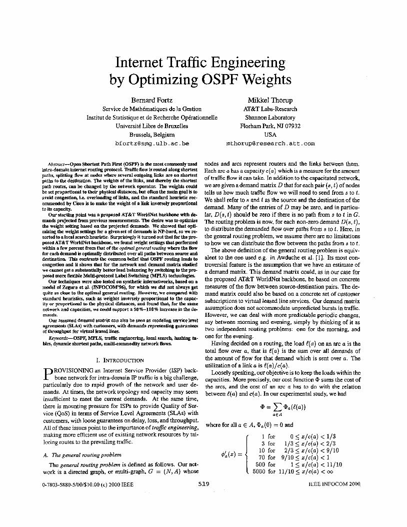
fig. 1. Arccost @,(!(a)) asafunctionofloadt(a) forarccapacityc(a) = 1.

The function !Da is illustrated in Fig. 2. The idea behind Qa is that it is cheap to send flow over an arc with a small utilization. As the utilization approaches loo%, it becomes more expensive, for example because we get more sensitive to bursts. If the utilization goes above loo%, we get heavily penalized, and when the utilization goes above 110% the penalty gets so high that this should never happen.

The exact definition of the objective function is not so important for our techniques, as long as it is a a piece-wise linear increasing and convex function.

PropositionI: If each @a is a piece-wise linear increasing and convex function, we can solve the general routing problem optimally in polynomial time.

Knowing the optimal solution for the general routing problem is an important benchmark for judging the quality of solutions based on, say, OSPF routing.

The above objective function provides a general best effort measure. We have previously claimed that our approach can also be used if the demand matrix is modeling service level agreements (SLAs) with customers, with demands representing guarantees of throughput for virtual leased lines. In this case, we are more interested in ensuring that no packet gets sent across overloaded arcs, so our objective is to minimize a maximum rather than a sum over the arcs. However, due to the very high penalty for overloaded arcs, our objective function favours solutions without overloaded arcs. A general advantage to working with a sum rather than a maximum is that even if there is a bottleneck link that is forced to be heavily loaded, our objective function still cares about minimizing the loads in the rest of the network.

B. OSPF versus MPLS routing protocols

Unfortunately, most intra-domain internet routing protocols today do not support a free distribution of flow between source and destination as defined above in the general routing problem. The most common protocol today is Open Shortest Path First (OSPF) [2]. In this protocol, the network operator assigns a weight to each link, and shortest paths from each router to each destination are computed using these weights as lengths of the links. In each router, the next link on all shortest paths to all possible destinations is stored in a table, and a demand going in the router is sent to its destination by splitting the flow between the links that are on the shortest paths to the destination. The exact mechanics of the splitting can be somewhat compli- cated, depending on the implementation. Here, as a simplifying approximation, we assume that it is an even split.

The quality of OSPF routing depends highly on the choice of weights. Nevertheless, as recommended by Cisco [3], these are often just set inversely proportional to the capacities of the links, without taking any knowledge of the demand into account.

It is widely believed that the OSPF protocol is not flexible enough to give good load balancing as defined, for example, in our objective function. This is one of the reasons for introducing the more flexible Multi-protocol Label Switching (MPLS) technologies ([l]. [4]). With MPLS one can in principle decide the path for each individual packet. Hence, we can simulate a solution to the general routing problem by distributing the packets on the paths between a source-destination pair using the same distribution as we used for the flow. The MPLS technology has some disadvantages. First of all, MPLS is not yet widely de- ployed, let alone tested. Second OSPF routing is simpler in the sense that the routing is completely determined by one weight for each arc. That is, we do not need to make individual routing decisions for each sourcddestination pair. Also, if a link faild, the weights on the remaining links immediately determines the new routing.

C. Our results

The general question studied in this paper is: Can a suj- jiciently clever weight settings make OSPF muting perfo+ nearly as well as optimal generaUMPL3 routing?

Our first answer is negative: for arbitrary n, we construct instance of the routing problem on 8 n3 nodes where any OSPF routing has its average flow on arcs with utilization Q(n) timds

With our concrete objective function, this demonstrates a gap of a factor approaching 5000 between the cost of the optimal general routing and the cost of the optimal OSPF routing.

The next natural question is: how well does OSPF routing perform on real networks. In particular we wanted to answer this question for a proposed AT&T WorldNet backbone. In addition, we studied synthetic intemetworks, generated as suggested by Calvert, Bhattacharjee, Daor, and Zegura 151, [6]. Finding a perfect answer is hard in the sense that it is NP-hard to find an optimal setting of the OSPF weights for an arbitrary network. Instead we resorted to a local search heuristic, not guaranteed to find optimal solutions. Very surprisingly, it turned out that for the proposed AThT WorldNet backbone, the heuristic found weight settings making OSPF routing performing within a few percent from the optimal general routing. Thus for the proposed AT&T WorldNet backbone with our projected demands, y d with our concrete objective function, there would be no sub-

well-tested and understood robust OSPF technology to the nefw MPLS alternative.

For the synthetic networks, we did not always get quite as close to the optimal general routing. However, we compared o b local search heuristic with standard heuristics, such as weights inversely proportional to the capacities or proportional to the physical distances, and found that, for the same network abd capacities, we could support a 50%-110% increase in the demands, both with respect to our concrete cost function and, simultaneously, and with respect to keeping the max-utilization below 100%.

i

f

higher than the max-utilization in an optimal general solution. 1

I I

stantial traffic engineering gain in switching from the existing I

I

t


D. Technical contributions lated as the following linear program.

mina =E ,EA

subject to

Our local search heuristic is original in its use of hash tables to avoid cycling and for search diversification. A first attempt of using hashing tables to avoid cycling in local search was made by Woodruff and Zemel [7] , in conjunction with tabu search. Our approach goes further and avoids completely the problem specific definitions of solution attributes and tabu mechanisms, leading to an algorithm that is conceptually simpler, easier to implement, and to adapt to other problems.

Our local search heuristic is also original in its use of more ad- vanced dynamic graph algorithms. Computing the OSPF routing resulting from a given setting of the weights tumed out to be the computational bottleneck of our local search algorithm, as many different solutions are evaluated during a neighborhood exploration. However, our neighborhood structure allows only a few local changes in the weights. We therefore developed efficient algorithms to update the routing and recompute the cost of a solution when a few weights are changed. These speed-ups are critical for the local search to reach a good solution within reasonable time bounds.

E. Contents

In Section I1 we formalize our general routing model as a linear program, thereby proving Proposition 1. We present in Sec- tion I11 a scaled cost function that will allow us to compare costs across different sizes and topologies of networks. In Section IV. a family of networks is constructed, demonstrating a large gap between OSPF and multi-commodity flow routing. In Section V we present our local search algorithm, guiding the search with hash tables. In Section VI we show how to speed-up the calcula- tions using dynamic graph algorithms. In Section VII, we report the numerical experiments. Finally, in Section VI11 we discuss our findings.

Because of space limitations, we defer to the journal version the proof that it is NP-hard to find an optimal weight setting for OSPF routing. In the journal version, based on collaborative work with Johnson and Papadimitriou, we will even prove it NP- hard to find a weight setting getting within a factor 1.77 from optimality for arbitrary graphs.

11. MODEL

A. Optimal routing

Recall that we are given a directed network G = (NI A ) with a capacity C ( U ) for each a E A. Furthermore, we have a demand matrix D that for each pair (s, t ) E N x N tells the demand D(s , t ) in traffic flow between s and t . We will sometimes refer to the non-zero entries of D as the demands. With each pair (s, t ) and each arc a, we associate a variable f i S l t ) telling how much of the traffic flow from s to t goes over a. Variable )(a) represents the total load on arc a, i.e. the sum of the flows going over a , and @, is used to model the piece-wise linear cost function of arc a.

With this notation, the general routing problem can be formu-

a E A , ( 8 , t ) E N x N

@a L e(a) a E A , (3) 0, 2 s e ( 4 - $ c ( u ) a E A , (4)

0, 2 7 0 t ( a ) - ?.(a) a E A , (6) oa 2 ioe(a) - g+) a EA, (5)

0, 2 500l(a) - y c ( a ) a E A , (7)

@a 2 50ooe(~) - YC(U) a E A , (8) ( 8 J ) > 0 fa - a € A; s , t E N . (9)

Constraints (I) are flow conservation constraints that ensure the desired traffic flow is routed from s to t , constraints (2) define the load on each arc and constraints (3) to (8) define the cost on each arc.

The above program is a complete linear programming for- mulation of the general routing problem, and hence it can be solved optimally in polynomial time (JShachiyan [SI), thus set- tling Proposition 1. In our experiments, we solved the above problems by calling CPLEX via AMPL. We shall use @OPT to denote the optimal general routing cost.

B. OSPF routing

In OSPF routing, we choose a weight w(a) for each arc. The length of a path is then the sum of its arc weights, and we have the extra condition that all flow leaving a node aimed at a given a destination is evenly spread over arcs on shortest paths to that destination. More precisely, for each source- destination pair (s, t) E N x N and for each node I, we have that f[:;:) = 0 if (t, y) is not on a shortest path from s to t ,

and that f[i:i\ = f[;:%, if both (I, y) and (2, y') are on shortest paths from s to t . Note that the routing of the demands is completely determined by the shortest paths which in turn are determined by the weights we assign to the arcs. Unfortunately, the above condition of splitting between shortest paths based on variable weights cannot be formulated as a linear program, and this extra condition makes the problem NP-hard.

We shall use O o p t ~ s p ~ to denote the optimal cost with OSPF routing.

111. NORMALIZING COST

We now introduce a normalizing scaling factor for the cost function that allows us to compare costs across different sizes and topologies of networks. To define the measure, we introduce

@Uncop = C ( D ( s , t ) .distl(s,t)). (10) ( s , t ) E N x N

IEEE INFOCOM 2000 0-7803-5880-5/00/$10.00 (c) 2000 IEEE 521

Above distl(.) is distance measured with unit weights (hop count). Also, we let @ u , i t ~ ~ p ~ denote the cost of OSPF routing with unit weights. Below we present several nice properties of @uncap and CPUnjtOSPF. It is (ii) that has inspired the name "Uncapacitated".

(i) @uncap is the total load if all traffic flow goes along unit weight shortest paths. (ii) @uncap = cPun;tOSpF if all arcs have unlimited capacity. (iii) @uncap is the minimal total load of the network. (iv) @uncap L @OPT.

Above, 5000 is the maximal value of CP;. PmoJ Above (i) follows directly from the definition. Now

(ii) follows from (i) since the ratio of cost over load on an arc is 1 if the capacity is more than 3 times the load. Further (iii) follows from (i) because sending flow along longer paths only increases the load. From (iii) we get (iv) since 1 is the smallest possible ratio of cost over load. Finally we get (v) from (ii) since decreasing the capacity of an arc with a given load increases the arc cost with strictly less than a factor 5000 if the capacity stays

Our scaled cost is now defined as:

Lemma 2:

(VI QunitOSPF < 5000 . @uncap.

positive.

From Lemma 2 (iv) and (v). we immediately get:

Note that if we get @* = 1, it means that we are routing along unit weight shortest paths with all loads staying below 1/3 of the capacity. In this ideal situation there is no point in increasing the capacities of the network.

A packet level view

Perhaps the most instructive way of understanding our cost functions is on the packet level. We can interpret the demand D(s , t ) as measuring how many packets - of identical sizes - we expect to send from s to t within a certain time frame. Each packet will follow a single path from s to t , and it pays a cost for each arc it uses. With our original cost function '9, the per packet cost for using an arc is 0, (e( .))/e( U ) . Now, CP can be obtained by summing the path cost for each packet.

The per packet arc cost @a(!(Cl))/e(Q) is a function q5 of the utilization L(a ) / c (u ) . The function 4 is depicted in Fig. 2. First is 1 while the utilization is 5 1/3. Then q5 increases to 10 - 16/3 = l o $ for a full arc, and after that it grows rapidly towards 5000. The costfactor of a packet is the ratio of its current cost over the cost it would have paid if it could follow the unit-weight shortest path without hitting any utilization above 1/3, hence paying the minimal cost of 1 for each arc traversed. The latter ideal situation is what is measured by @uncap, and therefore CP* measures the weighted average packet cost factor where each packet is weighted proportionally to the unit-weight distance between its end points.

If a packet follows a shortest path, and if all arcs are exactly full, the cost factor is exactly lo$. The same cost factor can of course be obtained by some arcs going above capacity and

i ",,,oz.,,,- - ' 1 - O P 01

Fig. 2. Arc packet cost as function of utilization

I I

Hg. 3. Gap between general flow solution on the left and OSPF solution on thei ! right

i others going below, or by the packet following a longer detouri using less congested arcs. Nevertheless, it is natural to say thad a routing congests a network if cP* 2 10;. 1

i

Iv. MAXIMAL GAP BETWEEN OPT AND OSPF

From (12), it follows that the maximal gap between optimal general routing and optimal OSPF routing is less than a factor 5000. In Lemma 3, we will now show that the gap can in fact apd proach 5000. Our proof is based on a construction where OSPF leads to very bad congestion for any natural definition of congestion. More precisly, for arbitrary n, we construct an instances of the routing problem on M n3 nodes with only one demand, and where all paths from the source to the destination are shortest with respect to unit weights, or hop count. In this instance, any OSPF routing has its average flow on arcs with utilization Q(n) times higher than the max-utilization in an optimal general solution. With our concrete objective function, this demonstrates a gap of a factor approaching 5000 between the cost of the optimal general routing and the cost of the optimal OSPF routing.

Lemma 3: There is a family of networks G, so that the opti, mal general routing approaches being 5000 times better than thF r optimal OSPF routing as n + 00. 1

?

Proof: In our construction, we have only one demand wi$ source s and destination t , that is, D ( z , y) > 0 if and only !f (cI y) = ( s , t ) . The demand is n. Starting from s, we have :a directed path P = (s I 2 1 I . . . 2,) where each arc has capacity 372. For each i, we have a path Qj of length n2 - i from z i to t . Thus, all paths from s to t have length n2. Each arc in each Q; has capacity 3. The graph is illustrated in Fig. 3 with P being the thick high capacity path going down on the left side.

In the general routing model, we send the flow down P , let- ting 1 unit branch out each Qi. This means that no arc gets more flow than a third of its capacity, so the optimal cost @zpT

0-7803-5880-5/00/$10.00 (c) 2000 IEEE 522 IEEE lNFOCOM 2000

satisfies

@zPT 5 n(n2 + n ) = (1 + o(1))n3.

In the OSPF model, we can freely decide which Qi we will use, but because of the even splitting, the first Qi used will get half the flow, i.e. n / 2 units, the second will get n/4 units, etc. Asymptotically this means that almost all the flow will go along arcs with load a factor Q ( n ) above their capacity, and since all paths uses at least n2 - n arcs in some Qi, the OSPF cost (P;;l,tOSPF satisfies

@zptOSPF 2 ( 1 - o(1))5000n3.

We conclude that the ratio of the OSPF cost over the optimal cost is such that '%izF 2 ( 1 - o( 1))5000 --+ 5000 as n 3 00. m

V. OSPF WEIGHT SETTING USING LOCAL SEARCH

A. Overview of the local search heuristic In OSPF routing, for each arc Q E A, we have to choose

a weight wa. These weights uniquely determine the shortest paths, the routing of traffic flow, the loads on the arcs, and finally, the cost function a. In this section, we present a local search heuristic to determine a weights vector (Wa)aEA that minimizes 0. We let W := { 1, . . . , wmaz} denote the set of possible weights.

Suppose that we want to minimize a function f over a set X of feasible solutions. Local search techniques are iterative procedures in which a neighborhood N ( x ) X is defined at each iteration for the current solution x E X, and which chooses the next iterate x' from this neighborhood. Often we want the neighbor x' E n/(x) to improve on f in the sense that f(z') <

Differences between local search heuristics arise essentially from the definition of the neighborhood, the way it is explored, and the choice of the next solution from the neighborhood. De- scent methods consider the entire neighborhood, select an improving neighbor and stop when a local minimum is found. Meta-heuristics such as tabu search or simulated annealing allow non-improving moves while applying restrictions to the neighborhood to avoid cycling. An extensive survey of local search and its application can be found in Aarts and Lenstra [9].

In the remainder of this section, we first describe the neighborhood structure we apply to solve the weight setting problem. Second, using hashing tables, we address the problem of avoid- ing cycling. These hashing tables are also used to avoid repetitions in the neighborhood exploration. While the neighborhood search aims at intensifying the search in a promising region, it is often of great practical importance to search a new region when the neighborhood search fails to improve the best solution for a while. These techniques are called search diversification and are addressed at the end of the section.

f (2).

B. Neighborhood structure

A solution of the weight setting problem is completely char- acterized by its vector w of weights. We define a neighbor wr E N ( w ) of w by one of the two following operations ap- plied to w.

0-7803-5880-j/00/$10.00 ( c ) 2000 IEEE

Single weight change. This simple modification consists in changing a single weight in w. We define a neighbor w' of w for each arc Q E A and for each possible weight t E W\{wa) by setting wb = t and wl, = W b for all b # a. Evenly balancingjlows. Assuming that the cost function Qa () for an arc Q E A is increasing and convex, meaning that we want to avoid highly congested arcs. we want to split the flow as evenly as possible between different arcs. More precisely, consider a demand node t such that CJEN D(s, t ) > 0 and some part of the demand going to t goes through a given node 2. Intuitively, we would like OSPF routing to split the flow to t going through t evenly along arcs leaving t. This is the case if all the arcs leaving 2 belong to a shortest path from z to t . More precisely, if 21 , z2, . . . , xp are the nodes adjacent to 2, and if Pi is one of the shortest paths from xi to t , for i = 1 , . . . , p , as illustrated in Fig. 4, then we want to set w' such that

W{Z,Zl) + w'(P1) = W { Z , Z 2 ) + w"> + 4 P P ) . - - . - ...-

where ~ ' ( p i ) denotes the sum of the weights of the arcs belong- ing to Pi. A simple way of achieving this goal is to set

w* - w(Pj) if a = (x, ti), fori = 1,. . . , p , { otherwise. w; =

where w* = 1 + maxi=1, , p { ~ ( P , ) } . A drawback of this approach is that an arc that does not belong to one of the shortest paths from t to t may already be congested, and the modifications of weights we propose will send more flow on this congested arc, an obviously undesirable feature. We therefore decided to choose at random a threshold ratio 0 between 0.25 and 1, and we only modify weights for arcs in the maximal subset B of arcs leaving x such that

w(c,zc) + pi) I ~ ( z , z ~ ) + w(pj) V i E B , j B, l ( s , z , ) ( ~ ) <_ 0 ~ ( z , zi) V i E B.

In this way, flow going from n to t can only change for arcs in B, and choosing 0 at random allows to diversify the search. Another drawback of this approach is that it does not ensure that weights remain below wmaz. This can be done by adding the condition that ma?riEB w(Pi) - miniEB W(Pi) 5 Wmaz is satisfied when choosing B.

C. Guiding the search with hashing tables The simplest local search heuristic is the descent method that,

at each iteration, selects the best element in the neighborhood and stops when this element does not improve the objective function. This approach leads to a local minimum that is often far from the optimal solution of the problem, and heuristics allowing non-improving moves have been considered. Un- fortunately, non-improving moves can lead to cycling, and one must provide mechanisms to avoid it. Tabu search algorithms (Glover [IO]), for example, make use of a tabu list that records some attributes of solutions encountered during the recent iterations and forbids any solution having the same attributes.

We developed a search strategy that completely avoids cycling without the need to store complex solution attributes. The

IEEE INFOCOM 2000 523

Fig. 4. The second type of move tries to make all paths form a to t of equal length.

solutions to our problem are 1.1 [-dimensional integer vectors. Our approach maps these vectors to integers, by means of a hashing function h, chosen as described in [ll]. Let I be the number of bits used to represent these integers. We use a boolean table T to record if a value produced by the hashing function has been encountered. As we need an entry in T for each possible value returned by h, the size of T is 2'. In our implementation, I = 16. At the beginning of the algorithm, all entries in T are set to false. If w is the solution produced at a given iteration, we set T(h(w)) to true, and, while searching the neighborhood, we reject any solution w' such that T(h(w' ) ) is true.

This approach completely eliminates cycling, but may also reject an excellent solution having the same hashing value as a solution met before. However, if h is chosen carefully, the probability of collision becomes negligible. A first attempt of using hashing tables to avoid cycling in local search was made by Woodruff and Zemel [7 ] , in conjunction with tabu search. It differs from our approach since we completely eliminate the tabu lists and the definition of solution attributes, and we store the values for all the solutions encountered, while Woodruff and Zemel only record recent iterations (as in tabu search again). Moreover, they store the hash values encountered in a list, leading to a time linear in the number of stored values to check if a solution must be rejected, while with our boolean table, this is done in constant time.

D. Speeding up neighborhood evaluation

Due to our complex neighborhood structure, it turned out that several moves often lead to the same weight settings. For efficiency, we would like to avoid evaluation of these equivalent moves. Again, hashing tables are a useful tool to achieve this goal : inside a neighborhood exploration, we define a secondary hashing table used to store the encountered weight settings as above, and we do not evaluate moves leading to a hashing value already met.

The neighborhood structure we use has also the drawback that the number of neighbors of a given solution is very large, and exploring the neighborhood completely may be too time consuming. To avoid this drawback, we only evaluate a randomly selected set of neighbors.

We start by evaluating 20 % of the neighborhood. Each time

the current solution is improved, we divide the size of the sampling by 3, while we multiply it by 10 each time the current solution is not improved. Moreover, we enforce sampling at least 1 % of the neighborhood.

E. Diversocation

Another important ingredient for local search efficiency is diversification. The aim of diversification is to escape from regions that have been explored for a while without any improve- ment, and to search regions as yet unexplored.

In our particular case, many weight settings can lead to the same routing. Therefore, we observed that when a local minimum is reached, it has many neighbors having the same cost, leading to long series of iterations with the same cost value. To escape from these "long valleys" of the search space, the secondary hashing table is again used. This table is generally reset at the end of each iteration, since we want to avoid repetitions inside a single iteration only. However, if the neighborhood exploration does not lead to a solution better than the current one, we do not reset the table. If this happens for several iterations, more and more collisions will occur and more potentially good solutions will be excluded, forcing the algorithm to escape from the region currently explored. For these collisions to appear at a reasonable rate, the size of the secondary hashing table must be small compared to the primary one. In our experiments, its size is 20 times the number of arcs in the network.

This approach for diversification is useful to avoid regions with a lot of local minima with the same cost, but is not suffi- cient to completely escape from one region and go to a possibly more attractive one. Therefore, each time the best solution found is not improved for 300 iterations, we randomly perturb the cur- ' rent solution in order to explore a new region from the search : space. The perturbation consists of adding a randomly selected i perturbation, uniformly chosen between -2 and +2, to 10 % of the weights.

VI. COST EVALUATION

We will now first show how to evaluate our cost function for the static case of a network with a specified weight setting. Computing this cost function from scratch is unfortunately too time consuming for our local search, so afterwards, we will show how to reuse computations, exploiting that there are only few weight changes between a current solution and any solution in its neighborhood.

A. The static case

We are given a directed multigraph G = ( N , A ) with arc capacities { C a } a c A , demand matrix D, and weights {Wa}acA. For the instances considered, the graph is sparse with IAl = 0 (IN I). Moreover, in the weighted graph the maximal distance, between any two nodes is O( INI).

We want to compute our cost function a. The basic problem is to compute the loads resulting from the weight setting. Wel will consider one destination t at a time, and compute the totali flow from all sources s E N to t . This gives rise to a certain/ partial load 1: = CsEN fLs") for each arc. Having done th4 above computation for each destination t , we can compute the load 1, on arc a as ztGN 1; .


To compute the flow to t , our first step is to use Dijkstra’s algorithm to compute all distances to t (normally Dijkstra’s algorithm computes the distances away from some source, but we can just apply such an implementation of Dijkstra’s algorithm to the graph obtained by reversing the orientation of all arcs in G). Having computed the distance cl: to t for each node, we compute the set At of arcs on shortest paths tot , that is,

For each node 2, let IS: denote its outdegree in A t , i.e. d: = I{Y E N (X,Y) E AtN.

Observation 4: For all (y, z ) E A t ,

Using Observation 4, we can now compute all the loads l{y,z, as follows. The nodes y E N are visited in order of decreasing distance 4 to 1. When visiting a node y. we first set

for each (y, z ) E At. To see that the above algorithm works correctly, we note the

invariant that when we start visiting a node y, we have correct loads 1; on all arcs a leaving nodes coming before y. In particular this implies that all the arcs (2 y) entering y have correctly computed loads I fx ,Y) , and hence when visiting y, we compute the correct load ltY,=) for arcs (y, z) leaving y.

Using bucketing for the priority queue in Dijkstra’s algorithm, the computation for each destination takes O ( ( A ( ) = O(lN1) time, and hence our total time bound is O ( ( N I 2 ) .

B. The dynamic case

In our local search we want to evaluate the cost of many different weight settings, and these evaluations are a bottleneck for our computation. To save time, we will try to exploit the fact that when we evaluate consecutive weight settings, typically only a few arc weights change. Thus it makes sense to try to be lazy and not recompute everything from scratch, but to reuse as much as possible. With respect to shortest paths, this idea is already well studied (Ramalingam and Reps [12]), and we can apply their algorithm directly. Their basic result is that, for the re- computation, we only spend time proportional to the number of arcs incident to nodes x whose distance dk to t changes. In our experiments there were typically only very few changes, so the gain was substantial - in the order of factor 20 for a 100 node graph. Similar positive experiences with this laziness have been reported in Frigioni et al. [13].

The set of changed distances immediately gives us a set of “update” arcs to be added to or deleted from A t . We will now present a lazy method for finding the changes of loads. We will operate with a set M of “critical” nodes. Initially, M consists of all nodes with an incoming or outgoing update arc. We repeat the following until M is empty: First, we take the node y E M which maximizes the updated distance db and remove y from M . Second, set 1 = &(D(y,t) -t C(r,y)EAt Finally, for each (y, z ) E A t , where At is also updated, if I # ltv,zl, set l t u , 2 ) = 1 and add z to M .

= k(D(Y>t) $- C ( z , y ) E A * ‘ t ~ , y ) ) ’ Second we set 2tg, , ) =

To see that the above suffices, first note that the nodes visited are considered in order of decreasing distances. This follows because we always take the node at the maximal distance and because when we add a new node z to M , it is closer to t than the currently visited node y. Consequently, our dynamic algorithm behaves exactly as our static algorithm except that it does not treat nodes not in M . However, all nodes whose incoming or outgoing arc set changes, or whose incoming arc loads change are put in M , so if a node is skipped, we know that the loads around it would be exactly the same as in the previous evaluation.

VII. NUMERICAL EXPERIMENTS We present here our results obtained with a proposed AT&T

WorldNet backbone as well as synthetic internetworks. Besides comparing our local search heuristic (HeurOSPF)

with the general optimum (OPT), we compared it with OSPF routing with “oblivious” weight settings based on properties of the arc alone but ignoring the rest of the network. The oblivious heuristics are InvCapOSPF setting the weight of an arc inversely proportional to its capacity as recommended by Cisco [3], UnitOSPF just setting all arc weights to 1, L2OSPF setting the weight proportional to its physical Euclidean distance ( L z norm), and RandomOSPF, just choosing the weights randomly.

Our local search heuristic starts with randomly generated weights and performs 5000 iterations, which for the largest graphs took approximately one hour. The random starting point was weights chosen for RandomOSPF, so the initial cost of our local search is that of RandomOSPF.

The results for the AT&T WorldNet backbone with different scalings of the projected demand matrix are presented in Table I. In each entry we have the normalized cost @* introduced in Sec- tion HI. The normalized cost is followed by the max-utilization in parenthesis. For all the OSPF schemes, the normalized cost and ma-utilization are calculated for the same weight setting and routing. However. for OPT, the optimal normalized cost and the optimal max-utilization are computed independently with different routing. We do not expect any general routing to be able to get the optimal normalized cost and max-utilization simultaneously. The results are also depicted graphically in Fig- ure 5. The first graph shows the normalized cost and the hori- zontal line shows our threshold of 10: for regarding thenetwork as congested. The second graph shows the max-utilization.

The synthetic internetworks were produced using the gener- ator GT-ITM [14], based on a model of Calvert, Bhattachar- jee, Daor, and Zegura [SI, 161. This model places nodes in a unit square, thus getting a distance 6(x, y) between each pair of nodes. These distances lead to random distribution of 2-level graphs, with arcs divided in two classes: local access arcs and long distance arcs. Arc capacities were set equal to 200 for local access arcs and to 1000 for long distance arcs. The above model does not include a model for the demands. We decided to model the demands as follows. For each node x , we pick two random numbers O,, Dy E [0,1] . Further, for each pair (z, y) of nodes we pick a random number C(,,y! E [0,1]. Now, if theEuclidean distance (L2) between x and y IS 6 ( x , y), the demand between x and y is

cUOxD, c ( x , y ) e - + ~ y ) ’ ~ A

IEEE INFOCOM 2000 0-7803-j880-5/00/$I0.00 (c) 2000 IEEE 525

Here a is a parameter and A is the largest Euciidean distance between any pair of nodes. Above, the 0, and D, model that different nodes can be more or less active senders and receivers, thus modelling hot spots on the net. Because we are multiplying three random variables, we have a quite large variation in the demands. The factor e-6(rpy)/3A implies that we have relatively more demand between close pairs of nodes. The results for the synthetic networks are presented in Figures 6 9 .

VIII. DISCUSSION

First consider the results for the AT&T WorldNet backbone with projected (non-scaled) demands in Table 5(*). As men- tioned in the introduction, our heuristic, HeurOSPF, is within 2% from optimality. In contrast, the oblivious methods are all off by at least 15%.

Considering the general picture for the normalized costs in Figures 5-9, we see that L2OSi’F and RandomOSPF compete to be worst. Then comes InvCapOSPF and UnitOSPF closely together, with InvCapOSPF being slightly better in all the figures but Figure 6. Recall that InvCapOSPF is Cisco’s recom- mendation [3], so it is comforting to see that it is the better of the oblivious heuristics. The clear winner of the OSPF schemes is our HeurOSPF, which is, in fact, much closer to the general optimum than to the oblivous OSPF schemes.

To quantify the difference between the different schemes, note that all curves, except those for RandomOSPF, start off pretty flat, and then, quite suddenly, start increasing rapidly. This pattern is somewhat similar to that in Fig. 1. This is not surprising since Fig. 1 shows the curve for a network consisting of a single arc. The reason why RandomOSPF does not follow this pattern is that the weight settings are generated randomly for each entry. The jumps of the curve for Random in Figure 8 nicely illustrate the impact of luck in the weight setting. In- terestingly, for a particular demand, the value of RandomOSPF is the value of the initial solution for our local search heuristic. However, the jumps of RandomOSPF are not transferred to HeurOSPF which hence seems oblivious to the quality of the initial solution.

Disregarding RandomOSPF, the most interesting comparison between the different schemes is the amount of demand they can cope with before the network gets too congested. In Section III. we defined lo$ as the threshold for congestion, but the exact threshold is inconsequential. In our experiments, we see that HeurOSPF allows us to cope with 50%-110% more demand. Also, in all but Figure 7, HeurOSPF is less than 2% from being able to cope with the same demands as the optimal general routing OPT. In Figure 7, HeurOSPF is about 20% from OPT. Recall that it is NP-hard even to approximate the optimal cost of an OSPF soIution, and we have no idea whether there ex- isits OSPF solutions closer to OPT than the ones found by our heuristic.

If we now turn out attention to the max-utilization, we get the same ordering of the schemes, with InvCapOSPF the winner among the oblivious schemes and HeurOSPF the overall best OSPF scheme. The step-like pattern of HeurOSPF show the impact of the changes in a:. For example, in Figure 5, we see how HeurOSPF fights to keep the max utilization below 1, in order to avoid the high penalty for getting load above capacity.

Following the pattern in our analysis for the normalized cost, we can ask how much more demand we can deal with before getting max-utiliztion above 1, and again we see that HeurOSPF beats the oblivious schemes with at least 50%.

The fact that our HeurOSPF provides weight settings and routings that are simultaneously good both for our best effort type average cost function, and for the performance guarantee type measure of max-utilization indicates that the weights obtained are “universally good” and not just tuned for our particular cost function. Recall that the values for OPT are not for the same routings, and there may be no general routing getting simultaneously closer to the optimal cost and the optimal max- utilization than HeurOSPF. Anyhow, our HeurOSPF is generally so close to OPT that there is only limited scope for improve- ment.

In conclusion, our results indicate that in the context of known demands, a clever weight setting algorithm for OSPF routing is a powerful tool for increasing a network’s ability to honor increasing demands, and that OSPF with clever weight setting can provide large parts of the potential gains of traffic engineering for supporting demands, even when compared with the possibil- ities of the much more flexible MPLS schemes. Acknowledgment We would like to thank David Johnson and Jennifer Rexford for some very useful comments. The first au-1

! thor was sponsored by the AT&T Research Prize 1997. i

REFERENCES [l] D. 0. Awduche, 1. Malcolm, J. Agogbua, M. ODell, and

J. McManus, “Requirements for traffic engineering ove MPLS,” Network Working Group, Request for Comments! ht tp : / / search. iet f . org/ rf c/rf c2702. txt, Septembei 1999. i

[21 J. T. Moy. OSPF: Anatomy of an lnternet Routing Protocal, Addison{ Wesley, 1999.

[3] Cisco, Conjguring OSPF, 1997. [41 E. C. Rosen, A. Viswanathan. and R. Callon. “Mul-

tiprotocol label switching architecture,” Network Working Group, Intemet Draft (work in progress). http://search.ietf.org/intemet-drafts/draft- ietf-mpls-arch-06. txt, 1999. E. W. Zegura, K. L. Calvert, and S . Bhattachajee, “How to model an intemetwork:’ in Proc. 15th IEEE Conf on Computer Communications (INFOCOM), 1996, pp. 594-602.

[6] K. Calvert, M. Doar. and E. W. Zegura, “Modeling intemet topology:’ IEEE Communications Magazine, vol. 35, no. 6, pp. 160-163, June 1997.

[7] D. L. Woodruff and E. Zemel, “Hashing vectors for tabu search,” Annals ofOperationsResearch, vol. 41, pp. 123-137.1993.

[8] L. G. Khachiyan, “A polynomial time algorithm for linear programming,” DoW. Akad Nauk SSSR. vol. 244. pp. 1093-1096.1979.

[9] E. H. L. Aarts and J. K. Lenstra, Eds., Local Search in Combinatorial Op- timizarion, Discrete Mathematics and Optimization. Wiley-Interscience, Chichester, England, June 1997.

[lo] F. Glover, “Future paths for integer programming and links to artificidl intelligence:’ Computers & Operations Research, vol. 13. pp. 533-549, 1986.

[l 11 M. Dietzfelbibger, “Universal hashing and k-wise independent random variables via integer arithmetic without primes,” in Proc. 13th Symp. on Theoretical Aspects of Computer Science (STACS), LNCS 1046.1996, pp. 22-24, Springer.

[ 121 G. Ramalingam and T. Reps, “An incremental algorithm for a generaliza- tion of the shortest-path problem,” Jounal of Algorithms, vol. 21, no. 2,

[I31 D. Frigioni, M. Ioffreda, U. Nanni. and G. Pasqualone. “Experimenth analysis of dynamic algorithms for the single-source shortest path problem,” ACM Jounal ofExperimental Algoritlunics. vol 3, article 5.1998.

[I41 E. W. Zegura, “GT-lTIvf: Georgia tech internetwork topology models (software):’ http: / lwww. cc . gatech. edu/ f ac? Ellen.Zegura/gt-itm/gt-itm.tar.gz.

[5]

pp. 267-305,1996.

0-7803-S880-5/00/$10.00 (c) 2000 IEEE 526 IEEE INFOCOM 2000

http://search.ietf.org/intemet-drafts/draft

Demand 3709 7417

11 126 14835

(*) 18465 22252 25961 29670 33378 37087 40796 44504

HeurOSPF 1.00 (0.17) 1.00 (0.30) 1.01 (0.34) 1.05 (0.47) 1.16 (0.59) 1.32 (0.67) 1.49 (0.78) 1.67 (0.89) 1.98 (1.00) 2.44 (1.00) 4.08 (1.10)

15.86 (1.34)

InvCapOSPF 1.01 (0.15) 1.01 (0.30) 1.05 (0.45) 1.15 (0.60) 1.33 (0.75) 1.62 (0.90) 2.70 (1.05)

17.61 (1.20) 55.27 (1.35)

106.93 (1.51) 175.44 (1.66) 246.22 (1.81)

OPT 1.00 (0.10) 1.00 (0.19) 1.01 (0.29) 1.04 (0.39) 1.14 (0.48) 1.30 (0.58) 1.46 (0.68) 1.63 (0.77) 1.89 (0.87) 2.33 (0.97) 3.64 (1.06)

13.06 (1.16)

UnitOSPF 1.00 (0.15) 1.00 (0.31) 1.03 (0.46) 1.13 (0.62) 1.31 (0.77) 1.59 (0.92) 3.09 (1.08)

21.78 (1.23) 51.15 (1.39) 93.85 (1.54)

157.00 (1.69) 228.30 (1.85)

L2OSPF 1.13 (0.23) 1.15 (0.46) 1.21 (0.70) 1.42 (0.93) 5.47 (1.16)

44.90 (1.39) 82.93 (1.62)

113.22 (1.86) 149.62 (2.09) 122.56 (2.32) 294.52 (2.55) 370.79 (2.78)

TABLE I

RandomOSPF 1.12 (0.35) 1.91 (1.05) 1.36 (0.66)

12.76 (1.15) 59.48 (1.32) 86.54 (1.72)

178.26 (1.86) 207.86 (4.36) 406.29 (1.93) 476.57 (2.65) 658.68 (3.09) 715.52 (3.37)

AT&T'S PROPOSED BACKBONE WITH 90 NODES AND 274 ARCS AND SCALED PROJECTED DEMANDS, WITH (*) MARKING THE ORIGINAL UNSCALED

DEMAND.

1.4 - 1 4

OPT - 1 . 2 - 12

10

U

: e

6

4

2

0 0 10000 20000 30000 40000 50000 60000 0 10000 20000 30000 40000 50000 60000

demand demand

Fig. 5. ATBrT's proposed backbone with 90 nodes and 274 arcs and scaled projected demands.

14

12

10

U

6

4

2

I 0 1000 2000 3000 4000 5000 6000 7000

demand

1.4

1 . 2

..I B 1

a -2 0 .8

4 U z o'6 0 . 4

0 . 2

0

Fig. 6. 2-level graph with 50 nodes and 148 arcs.

0-7803-5880-5/00/$10.00 ( c ) 2000 IEEE 527 IEEE INFOCOM 2000

LZOSPF 1.4 - 14

OPT - 12

10

u 8

6

:

4

2

0 0 1000 2000 3000 4000 5000 6000 0 1000 2000 3000 4000 5000 6000

demand demand

Fig. 7. 2-levelgraph with 50 nodes and 212 arcs.

InvCapOSPF ------- L20SPP --*--

RandomOSPF --*--- HeurOSPP -.-.e--

OPT - UnitOSpp

0 1000 2000 3000 4000 5000 6000 demand

14

12

10

U

6

1.4

1 . 2

8 1

.: 0 . 8

..-I

9

4 ..-I

i O b 6 0.4

0 . 2

0

InvCapOSPF .-. - - - - UnitOSPF

RandomOSPP HeurOSPF

L2OSPF

OPT -

1000 2000 3000 4000 5000 6000

demand


LZOSPF --.A -- RandomOSPF

? HeurOSPF --.e-.- - / !

t OPT - I

0 ' Ll 0 2000 4000 6000 8000 10000 12000 14000 16000 18000

1.4

1 . 2

0 . 2

n 0 2000 4000 6000 8000 10000 12000 14000 16000 18000

demand demand


0-7803-5880-5/00/$10.00 ( c ) 2000 IEEE IEEE INFOCOM 2000 528

internet traffic engineering by optimizing ospf weights - infocom

Documents