Image Enhancement(Point Processing)

(EE663 – Image Processing)

Dr. Samir H. Abdul-JauwadElectrical Engineering DepartmentCollege of Engineering Sciences

King Fahd University of Petroleum & MineralsDhahran – Saudi Arabiasamara@kfupm.edu.sa

Contents

•In this lecture we will look at image enhancement point processing techniques:

– What is point processing?– Negative images– Thresholding– Logarithmic transformation– Power law transforms– Grey level slicing– Bit plane slicing

Some Basic Relationships Between Pixels

• Definitions:

– f(x,y): digital image– Pixels: q, p– Subset of pixels of f(x,y): S

Neighbors of a Pixel

• A pixel p at (x,y) has 2 horizontal and 2 vertical neighbors:

– (x+1,y), (x-1,y), (x,y+1), (x,y-1)

– This set of pixels is called the 4-neighbors of p: N4(p)

Neighbors of a Pixel

• The 4 diagonal neighbors of p are: (ND(p))

– (x+1,y+1), (x+1,y-1), (x-1,y+1), (x-1,y-1)

• N4(p) + ND(p) N8(p): the 8-neighbors of p

Connectivity

• Connectivity between pixels is important:

– Because it is used in establishing boundaries of objects and components of regions in an image

Connectivity

• Two pixels are connected if:

– They are neighbors (i.e. adjacent in some sense -- e.g. N4(p), N8(p), …)

– Their gray levels satisfy a specified criterion of similarity (e.g. equality, …)

• V is the set of gray-level values used to define adjacency (e.g. V={1} for adjacency of pixels of value 1)

Adjacency

• We consider three types of adjacency:

– 4-adjacency: two pixels p and q with values from V are 4-adjacent if q is in the set N4(p)

– 8-adjacency : p & q are 8- adjacent if q is in the set N8(p)

Adjacency

• The third type of adjacency:

– m-adjacency: p & q with values from V are m-adjacent if

• q is in N4(p) or• q is in ND(p) and the set N4(p)N4(q) has no pixels with values

from V

Adjacency

• Mixed adjacency is a modification of 8-adjacency and is used to eliminate the multiple path connections that often arise when 8-adjacency is used.

100010110

100010110

100010110

Adjacency

• Two image subsets S1 and S2 are adjacent if some pixel in S1 is adjacent to some pixel in S2.

Path

• A path (curve) from pixel p with coordinates (x,y) to pixel q with coordinates (s,t) is a sequence of distinct pixels:

– (x0,y0), (x1,y1), …, (xn,yn)

– where (x0,y0)=(x,y), (xn,yn)=(s,t), and (xi,yi) is adjacent to (xi-1,yi-1), for 1≤i ≤n ; n is the length of the path.

• If (xo, yo) = (xn, yn): a closed path

Paths

• 4-, 8-, m-paths can be defined depending on the type of adjacency specified.

• If p,q � S, then q is connected to p in S if there is a path from p to q consisting entirely of pixels in S.

Connectivity

• For any pixel p in S, the set of pixels in S that are connected to p is a connected component of S.

• If S has only one connected component then S is called a connected set.

Boundary

• R a subset of pixels: R is a region if R is a connected set.

• Its boundary (border, contour) is the set of pixels in R that have at least one neighbor not in R

• Edge can be the region boundary (in binary images)

Distance Measures

• For pixels p,q,z with coordinates (x,y), (s,t), (u,v), D is a distance function or metric if:

– D(p,q) ≥ 0 (D(p,q)=0 iff p=q)– D(p,q) = D(q,p) and– D(p,z) ≤ D(p,q) + D(q,z)

Distance Measures

• Euclidean distance:

– De(p,q) = [(x-s)2 + (y-t)2]1/2

– Points (pixels) having a distance less than or equal to r from (x,y) are contained in a disk of radius r centered at (x,y).

Distance Measures

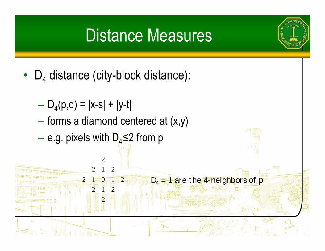
• D4 distance (city-block distance):

– D4(p,q) = |x-s| + |y-t|– forms a diamond centered at (x,y)– e.g. pixels with D4≤2 from p

2212

21012212

2

D4 = 1 are the 4-neighbors of p

Distance Measures

• D8 distance (chessboard distance):

– D8(p,q) = max(|x-s|,|y-t|)– Forms a square centered at p– e.g. pixels with D8≤2 from p

2222221112210122111222222

D8 = 1 are the 8-neighbors of p

Distance Measures

• D4 and D8 distances between p and q are independent of any paths that exist between the points because these distances involve only the coordinates of the points (regardless of whether a connected path exists between them).

Distance Measures

• However, for m-connectivity the value of the distance (length of path) between two pixels depends on the values of the pixels along the path and those of their neighbors.

Distance Measures

• e.g. assume p, p2, p4 = 1p1, p3 = can have either 0 or 1

ppp

pp

21

43

If only connectivity of pixels valued 1 is allowed, and p1 and p3 are 0, the m-

distance between p and p4 is 2.

If either p1 or p3 is 1, the distance is 3.

If both p1 and p3 are 1, the distance is 4 (pp1p2p3p4)

Basic Spatial Domain Image Enhancement

Origin x

y Image f (x, y)

(x, y)

•Most spatial domain enhancement operations can be reduced to the form•g (x, y) = T[ f (x, y)]•where f (x, y) is the input image, g (x, y) is the processed image and T is some operator defined over some neighbourhood of (x, y)

Point Processing

•The simplest spatial domain operations occur when the neighbourhood is simply the pixel itself•In this case T is referred to as a grey level transformation function or a point processing operation•Point processing operations take the form

•s = T ( r )•where s refers to the processed image pixel value and r refers to the original image pixel value

Point Processing Example: Negative Images

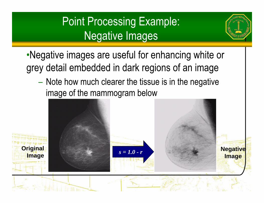
•Negative images are useful for enhancing white or grey detail embedded in dark regions of an image

– Note how much clearer the tissue is in the negative image of the mammogram below

s = 1.0 - rOriginal Image

Negative Image

Point Processing Example: Negative Images (cont…)

Original Image x

y Image f (x, y)

Enhanced Image x

y Image f (x, y)

s = intensitymax - r

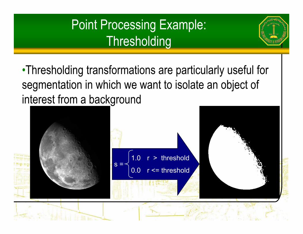
Point Processing Example: Thresholding

•Thresholding transformations are particularly useful for segmentation in which we want to isolate an object of interest from a background

s = 1.0

0.0 r <= threshold

r > threshold

Point Processing Example: Thresholding (cont…)

Original Image x

y Image f (x, y)

Enhanced Image x

y Image f (x, y)

s = 0.0 r <= threshold1.0 r > threshold

Intensity Transformations

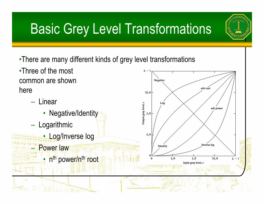
Basic Grey Level Transformations

•There are many different kinds of grey level transformations•Three of the most common are shown here

– Linear • Negative/Identity

– Logarithmic• Log/Inverse log

– Power law• nth power/nth root

Logarithmic Transformations

•The general form of the log transformation is •s = c * log(1 + r)

•The log transformation maps a narrow range of low input grey level values into a wider range of output values•The inverse log transformation performs the opposite transformation

Logarithmic Transformations (cont…)

•Log functions are particularly useful when the input grey level values may have an extremely large range of values•In the following example the Fourier transform of an image is put through a log transform to reveal more detail

s = log(1 + r)

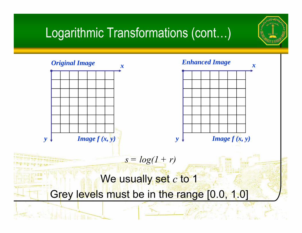
Logarithmic Transformations (cont…)

Original Image x

y Image f (x, y)

Enhanced Image x

y Image f (x, y)

s = log(1 + r)

We usually set c to 1Grey levels must be in the range [0.0, 1.0]

Power Law Transformations

Power law transformations have the following form

s = c * r γMap a narrow range of dark input values into a wider range of output values or vice versaVarying γ gives a whole family of curves

Power Law Transformations (cont…)

•We usually set c to 1•Grey levels must be in the range [0.0, 1.0]

Original Image x

y Image f (x, y)

Enhanced Image x

y Image f (x, y)

s = r γ

Power Law Example

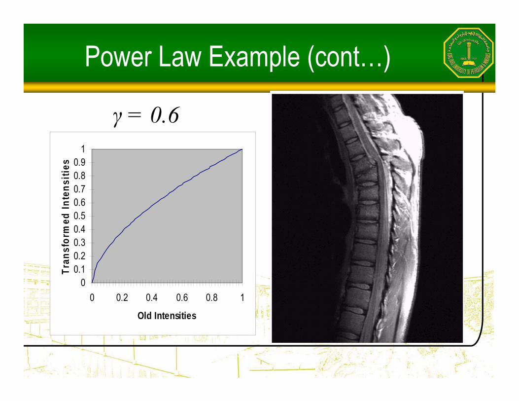
Power Law Example (cont…)

γ = 0.6

00.10.20.30.40.50.60.70.80.9

1

0 0.2 0.4 0.6 0.8 1

Old Intensities

Tran

sfor

med

Inte

nsiti

es

Power Law Example (cont…)

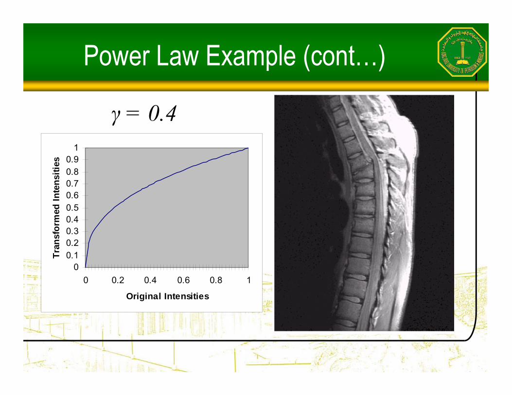
γ = 0.4

00.10.20.30.40.50.60.70.80.9

1

0 0.2 0.4 0.6 0.8 1

Original Intensities

Tran

sfor

med

Inte

nsiti

es

Power Law Example (cont…)

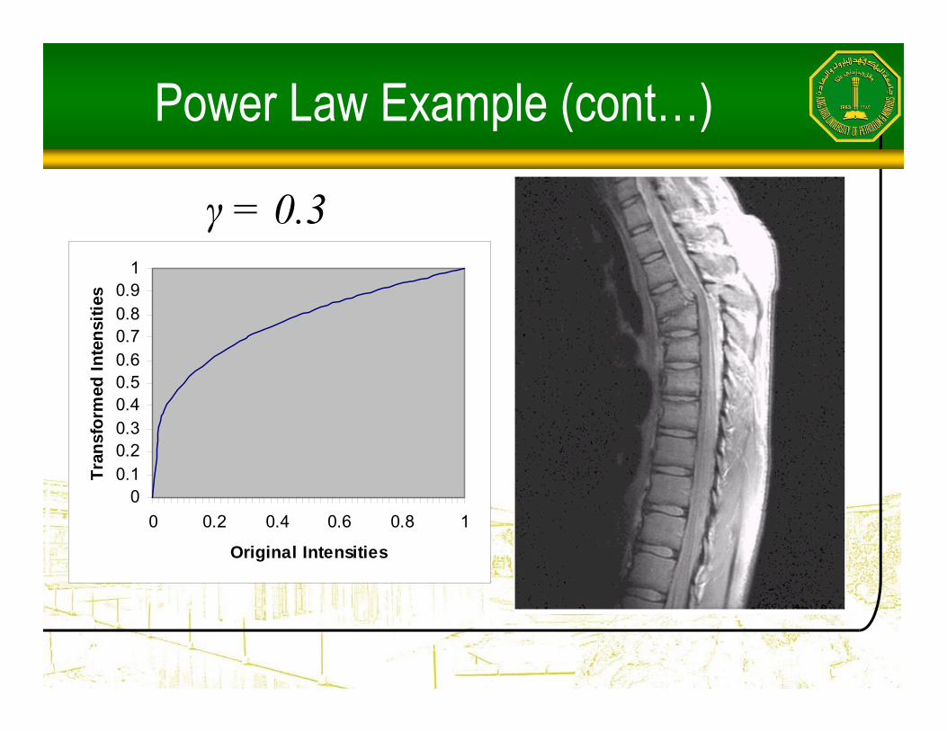
γ = 0.3

00.10.20.30.40.50.60.70.80.9

1

0 0.2 0.4 0.6 0.8 1

Original Intensities

Tran

sfor

med

Inte

nsiti

es

Power Law Example (cont…)

•The images to the right show a magnetic resonance (MR) image of a fractured human spine •Different curves highlight different detail

s = r 0.6

s = r 0.4

Power Law Example

Power Law Example (cont…)

γ = 5.0

00.10.20.30.40.50.60.70.80.9

1

0 0.2 0.4 0.6 0.8 1

Original Intensities

Tran

sfor

med

Inte

nsiti

es

Power Law Transformations (cont…)

•An aerial photo of a runway is shown•This time power law transforms are used to darken the image•Different curves highlight different detail

s = r 3.0

s = r 4.0

Gamma Correction

•Many of you might be familiar with gamma correction of computer monitors•Problem is thatdisplay devices do not respond linearly to different intensities•Can be corrected using a log transform

More Contrast Issues

Piecewise Linear Transformation Functions

•Rather than using a well defined mathematical function we can use arbitrary user-defined transforms•The images below show a contrast stretching linear transform to add contrast to a poor quality image

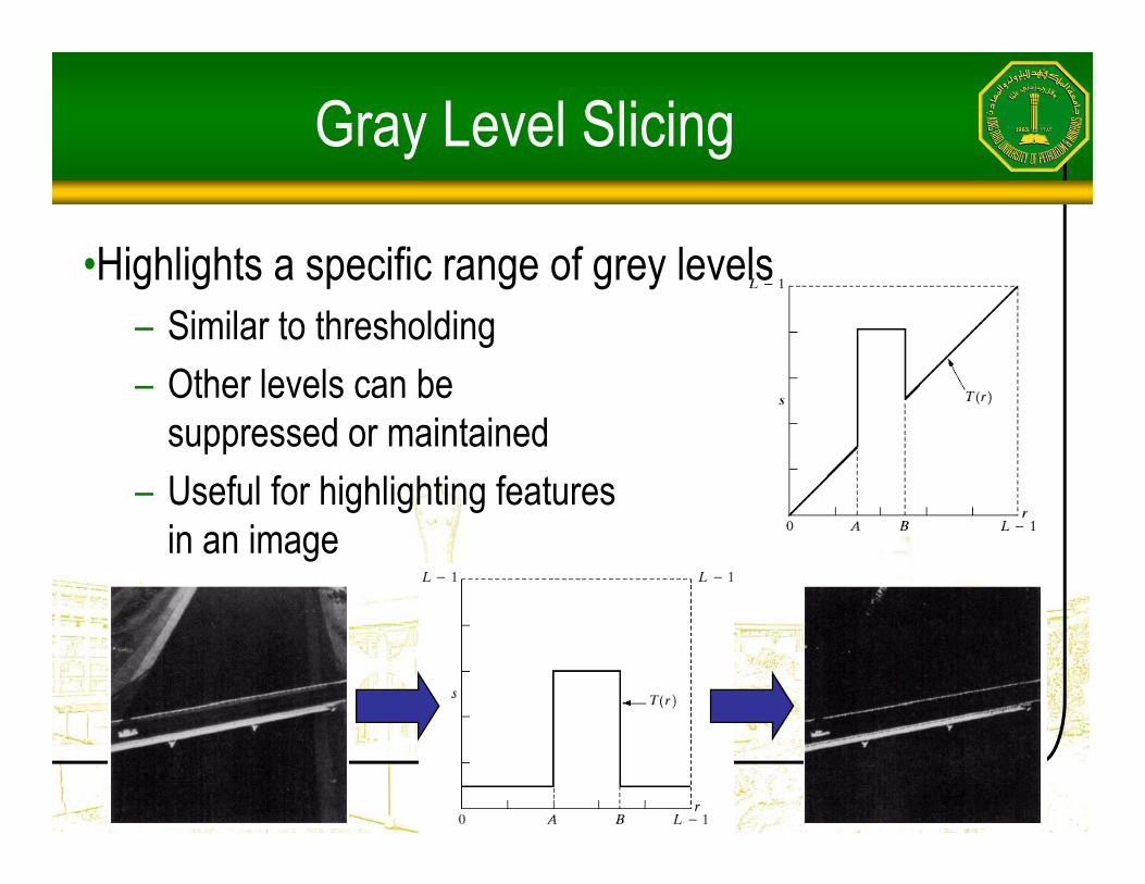
Gray Level Slicing

•Highlights a specific range of grey levels– Similar to thresholding– Other levels can be

suppressed or maintained– Useful for highlighting features

in an image

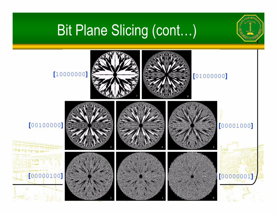
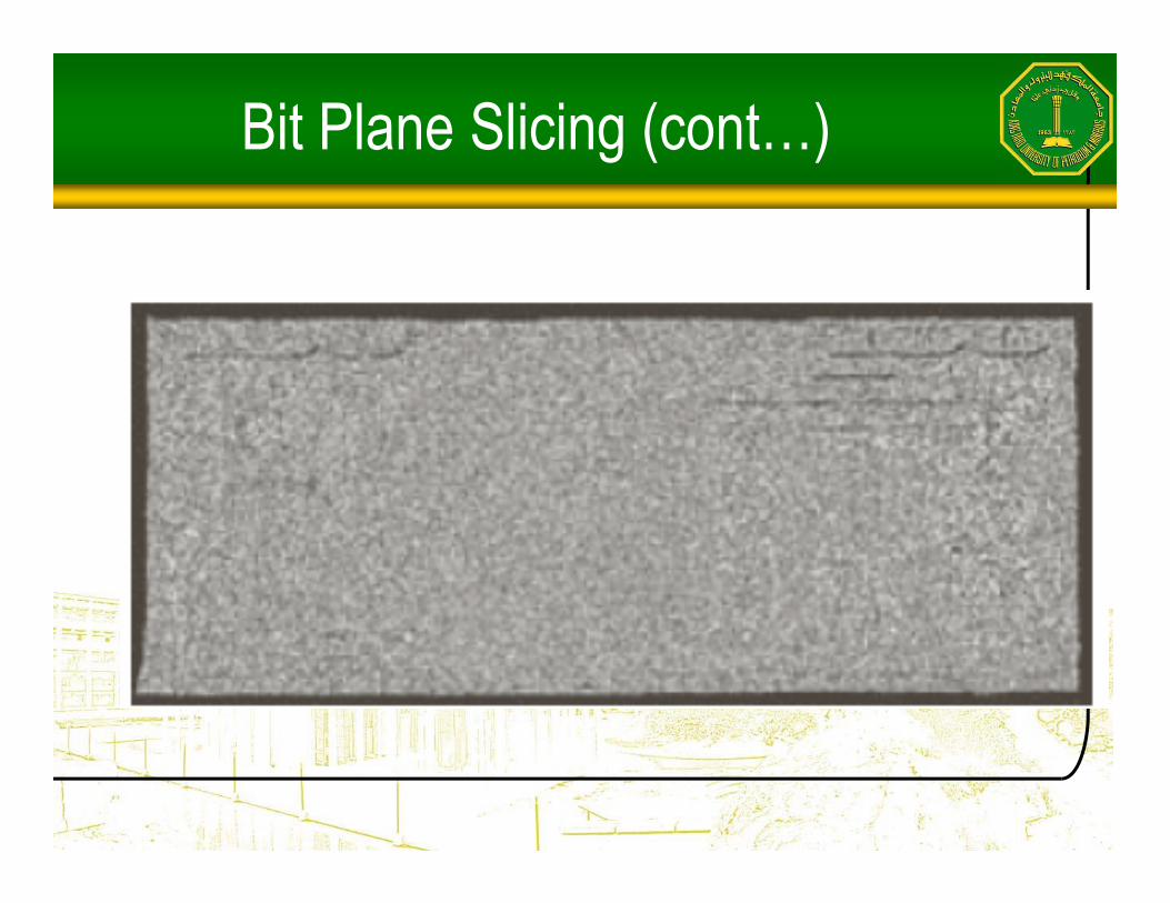
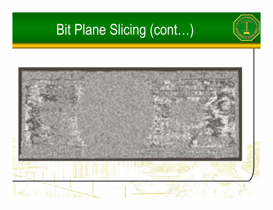
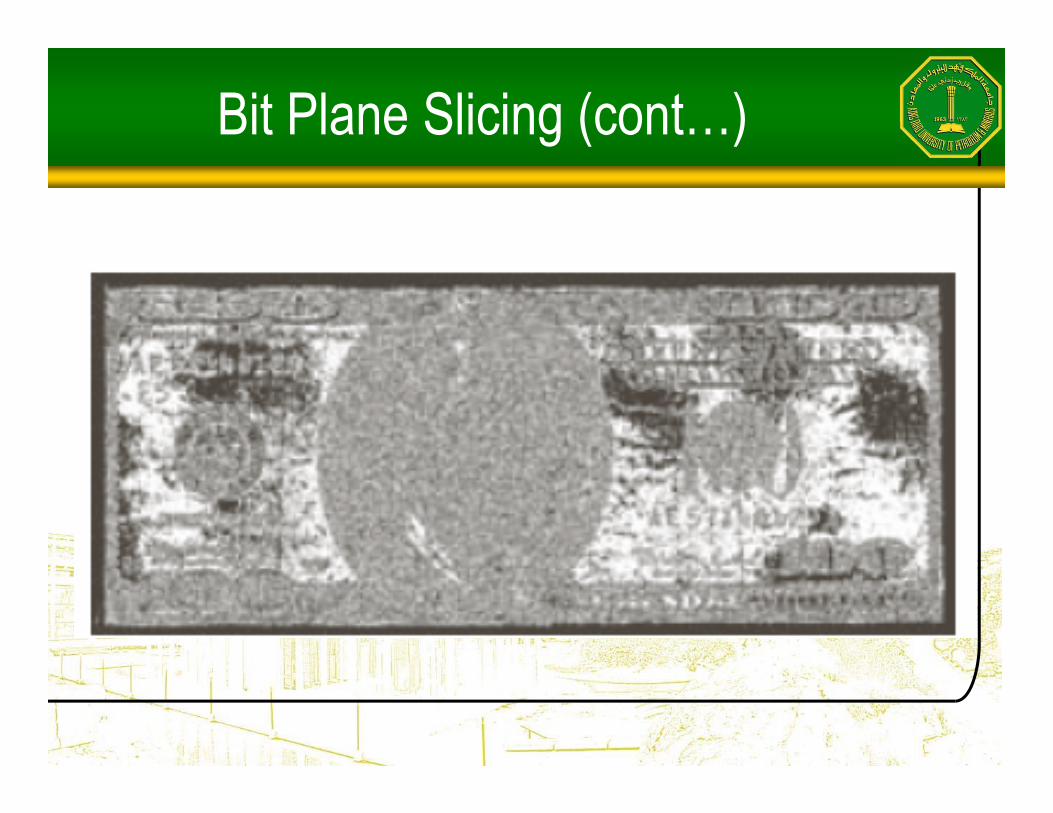
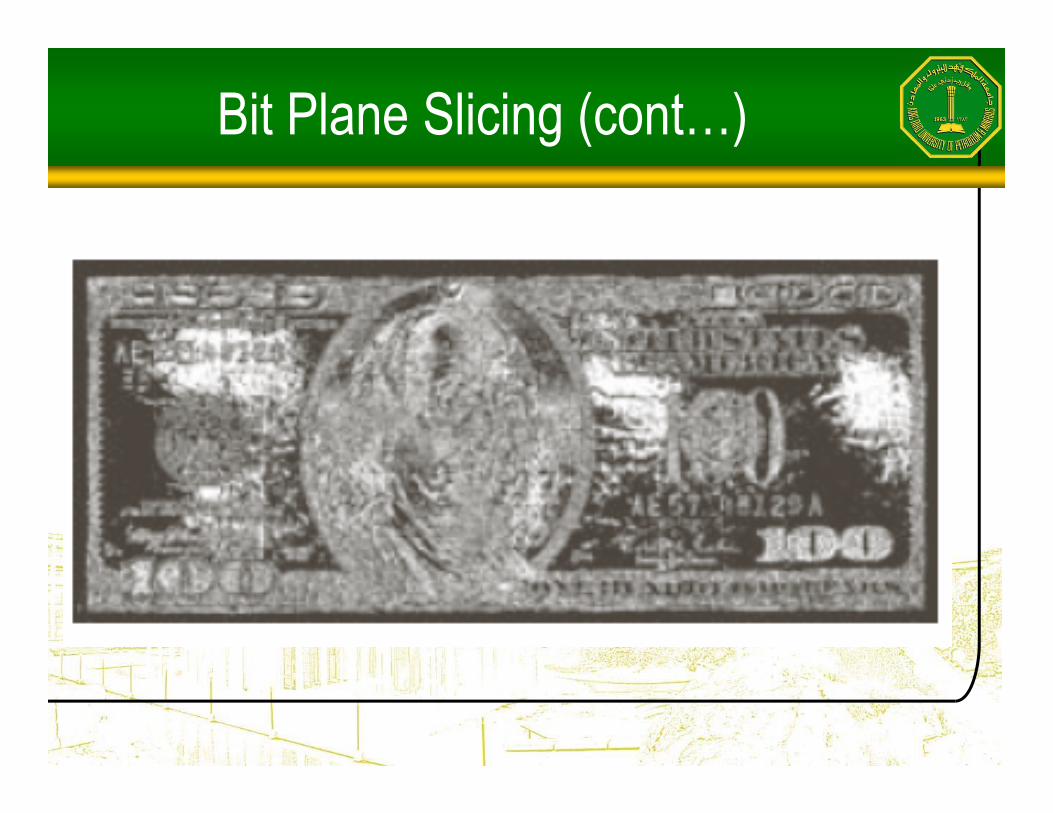
Bit Plane Slicing

•Often by isolating particular bits of the pixel values in an image we can highlight interesting aspects of that image

– Higher-order bits usually contain most of the significant visual information

– Lower-order bits containsubtle details

Bit Plane Slicing (cont…)

[10000000] [01000000]

[00100000] [00001000]

[00000100] [00000001]

Bit Plane Slicing (cont…)

[10000000] [01000000]

[00100000] [00001000]

[00000100] [00000001]

Bit Plane Slicing (cont…)

Bit Plane Slicing (cont…)

Bit Plane Slicing (cont…)

Bit Plane Slicing (cont…)

Bit Plane Slicing (cont…)

Bit Plane Slicing (cont…)

Bit Plane Slicing (cont…)

Bit Plane Slicing (cont…)

Bit Plane Slicing (cont…)

Bit Plane Slicing (cont…)

Bit Plane Slicing (cont…)

Reconstructed image using only bit planes 8

and 7

Reconstructed image using only bit planes 8, 7

and 6

Reconstructed image using only bit planes 7, 6

and 5

Summary

•We have looked at different kinds of point processing image enhancement