multi - kfupm
TRANSCRIPT

MULTI-OBJECTIVE OPTIMIZATION APPROACH TO SOFTWARE
PACKAGING USING SEQUENCE DIAGRAMS
ALIYU BAGUDU
COMPUTER SCIENCE
May 2017


iii
© Aliyu Bagudu
2017

iv
Dedicated to my mother

v
ACKNOWLEDGMENTS
I acknowledge, with deep gratitude and appreciation, the inspiration, encouragement,
valuable time and guidance given to me by Dr. Jameleddine Hassine, who served as my
advisor. Thereafter, I am deeply indebted and grateful to Dr. Moataz Ahmed, Dr. Sajjad
Mahmood, Dr. Ahmad Shouki, Dr. Abib, Mr Al-Helali Baligh Mohammed Ahmed, Mr.
Hayatullahi Bolaji Adeyamo, Mr. Mojeed Oyedeji
vi
TABLE OF CONTENTS
ACKNOWLEDGMENTS ............................................................................................................. V
TABLE OF CONTENTS ............................................................................................................. VI
LIST OF TABLES ......................................................................................................................... X
LIST OF FIGURES ................................................................................................................... XIII
LIST OF ABBREVIATIONS ..................................................................................................... XV
ABSTRACT ............................................................................................................................... XVI
XVII.............................................................................................................................. ملخص الرسالة
CHAPTER 1 INTRODUCTION ................................................................................................. 1
1.1 Motivation ...................................................................................................................................... 1
1.2 Problem Statement ......................................................................................................................... 3
1.3 Research Hypotheses ...................................................................................................................... 4
1.4 Thesis Approach .............................................................................................................................. 5
1.5 Thesis Contributions ....................................................................................................................... 5
1.6 Thesis Outline ................................................................................................................................. 6
CHAPTER 2 BACKGROUND .................................................................................................... 8
2.1 Multi-objective optimization........................................................................................................... 8
2.1.1 Solution space ............................................................................................................................ 9
2.1.2 Variable types .......................................................................................................................... 10
2.1.3 Local and global optimum ........................................................................................................ 11
2.1.4 Coping with problem hardness ................................................................................................. 13
2.1.5 Single and Multiple objective functions .................................................................................... 14
vii
2.1.6 Model evaluation and selection ............................................................................................... 18
2.2 Meta-heuristic optimization algorithms ........................................................................................ 19
2.2.1 Exploitation and Exploration .................................................................................................... 20
2.2.2 Genetic algorithm (GA) ............................................................................................................. 21
2.2.3 Covariance matrix adaptation-evolution strategy (CMA-ES) ..................................................... 21
2.2.4 Particle swarm optimization (PSO) ........................................................................................... 22
2.2.5 Differential evolution (DE) ........................................................................................................ 22
2.2.6 Performance assessment .......................................................................................................... 23
2.2.7 Parameters types ..................................................................................................................... 25
2.2.8 Parameter Search Techniques .................................................................................................. 26
2.3 Literature Review .......................................................................................................................... 26
2.3.1 Packaging quality metric .......................................................................................................... 26
2.3.2 Architectural stability metrics .................................................................................................. 30
CHAPTER 3 RESEARCH METHODOLOGY ........................................................................ 35
3.1 Fitness function for Functionality-based software packaging using sequence diagrams ................ 35
3.1.1 Degree of UC coverage ............................................................................................................. 40
3.1.2 Degree of class relevancy ......................................................................................................... 42
3.2 Problem solving ............................................................................................................................ 48
3.2.1 Model extension ...................................................................................................................... 48
3.2.2 Solution representation............................................................................................................ 50
3.2.3 Architectural stability ............................................................................................................... 53
CHAPTER 4 EMPIRICAL VALIDATION RESULTS........................................................... 56
4.1 Experiment Setup and Design ....................................................................................................... 56
4.1.1 System and platform ................................................................................................................ 56
viii
4.1.2 Experiment parameters ............................................................................................................ 56
4.1.3 Experiment design .................................................................................................................... 57
4.2 Solution representation experiments ........................................................................................... 57
4.2.1 49 bits representation .............................................................................................................. 59
4.2.2 7 integer representation ........................................................................................................... 60
4.2.3 1 integer rounded ..................................................................................................................... 61
4.2.4 1 integer configuration array .................................................................................................... 62
4.2.5 Discussion and conclusion: Solution representation ................................................................. 63
4.3 Model evaluation experiment ....................................................................................................... 63
4.3.1 Brute force analysis .................................................................................................................. 63
4.3.2 Convolution Neural Network model evaluation ....................................................................... 69
4.3.3 Packaging metric correlation with ASM, ExASM, and CEAM ..................................................... 74
4.4 Optimization algorithms experiment .......................................................................................... 101
4.4.1 Result optimization algorithms evaluation ............................................................................. 101
CHAPTER 5 CONCLUSION .................................................................................................. 106
5.1 Contributions and their implications ........................................................................................... 106
5.2 Threats to validity ....................................................................................................................... 107
5.2.1 Threats to construct validity ................................................................................................... 107
5.2.2 Threats to external validity ..................................................................................................... 108
5.2.3 Threats to Internal validity ..................................................................................................... 108
5.3 Future work ................................................................................................................................ 108
REFERENCES.......................................................................................................................... 110
APPENDIX 1: ASM, EXASM, CEAM CASES ILLUSTRATION ...................................... 115
APPENDIX 2: GA AND DE RESULTS ................................................................................ 166

ix
VITAE ....................................................................................................................................... 174
x
LIST OF TABLES
Table 1: Summary of the architetural stability metrics ......................................................34
Table 2: showing calculation of overall packaging of the system .....................................43
Table 3: 49 bits optimization result ...................................................................................59
Table 4: 7 integer optimization result ................................................................................60
Table 5: 1 integer optimization result ................................................................................61
Table 6: 1 integer confic array optimization result ............................................................62
Table 7: average score comparison ....................................................................................63
Table 8: Number of genotypes of a given phenotype with n number of packages ............65
Table 9: Number of phenotypes with given number of packages n ..................................66
Table 10: expert suggested rank compared with (Ebad & Ahmed, 2015) metric ............70
Table 11: CNN with linear activations unites ....................................................................72
Table 12: CNN with logistic activation unites ...................................................................73
Table 13: Results summary for ExASM different weights ................................................84
Table 14: ASM results summary .......................................................................................85
Table 15: ExASM results summary ...................................................................................86
Table 16: ASM results summary optimal packages ..........................................................88
Table 17: PgQlty vs CEAM correlation scenario 1 ...........................................................91
Table 18: PgQlty vs CEAM correlation scenario 2 ...........................................................93
Table 19: ChangeInPgQlty vs ChangeInCEAM correlation scenario 3 ............................95
Table 20: ChangeInPgQlty vs ChangeInCEAM correlation scenario 4 ............................96
Table 21: ExASM real case study results summary (w = 0.2)...........................................98
Table 22: : ExASM real case study results summary (w = 0.3) ........................................98
Table 23: : ExASM real case study results summary (w = 0.4) ........................................98
Table 24: : ExASM real case study results summary (w = 0.5) ........................................99
Table 25: : ExASM real case study results summary (w = 0.6) ........................................99
Table 26: GA parameters setting .....................................................................................102
Table 27: GA experiment result summary .......................................................................102
Table 28: DE parameters .................................................................................................103
Table 29: DE experiment result summary .......................................................................104
Table 30: CMAES parameters setting .............................................................................104
Table 31: CMAES experiment result summary ...............................................................105
Table 32: CMAES experiment result ...............................................................................105
Table 33: Case 1: ASM, ExASM, CEAM of v1.1 and v1.1 ............................................115
Table 34: Case 2: adding an inter-package call into V1.1 to make V2.1 ........................116
Table 35: Case 3: adding an intra-package call into V1.1 to make V3.1 ........................117
Table 36: Case 4: deleting an inter-package call from V1.1 to make V4.1 .....................118
Table 37: Case 5: deleting an intra-package call from V1.1 to make V5.1 .....................119
Table 38: Case 6: adding a class making inter-package call into V1.1 to makeV6.1 ......120
xi
Table 39: Case 7: adding a class making intra-package call into V1.1 to make V7.1 .....121
Table 40: Case 8: deleting a class making inter-package call from V1.1 to makeV8.1 ..122
Table 41: Case 9: deleting a class making intra-package call from V1.1 to makeV9.1 ..123
Table 42: Case 1: ASM of v1.1 and v1.1 .........................................................................124
Table 43: Case 1: ExASM of v1.1 and v1.1 ....................................................................125
Table 44: Case 2: ASM adding an inter-package call into V1.1 to make V2.1 ...............126
Table 45: Case 2: ExASM adding an inter-package call into V1.1 to make V2.1 ..........127
Table 46: Case 2: Top 2 configurations of V1.1 and V2.1 after optimization search as
(V1.2, V1.3) .....................................................................................................129
Table 47: Case 2: Top 2 configurations of V1.1 and V2.1 after optimization search as
(V2.2, V2.3) .....................................................................................................130
Table 48: Case 3: ASM adding an additional intra-package call into V1.1 to make
V3.1 .................................................................................................................131
Table 49: Case 3: ExASM adding an additional intra-package call into V1.1 to make
V3.1 .................................................................................................................132
Table 50: Case 3: Top 2 configurations of V1.1 and V3.1 after optimization search as
(V1.2, V1.3) .....................................................................................................134
Table 51: Case 3: Top 2 configurations of V1.1 and V3.1 after optimization search as
(V3.2, V3.3) .....................................................................................................135
Table 52: Case 4: ASM deleting an inter-package call from V1.1 as V4.1 .....................136
Table 53: Case 4: ExASM deleting an inter-package call from V1.1 as V4.1 ................137
Table 54: Case 4: Top 2 configurations of V1.1 and V4.1 after optimization search as
(V1.2, V1.3) .....................................................................................................139
Table 55: Case 4: Top 2 configurations of V1.1 and V4.1 after optimization search as
(V4.2, V4.3) .....................................................................................................140
Table 56: Case 5: ASM deleting an intra-package call from V1.1 to make V5.1 ...........141
Table 57: Case 5: ExASM deleting an intra-package call from V1.1 to make V5.1 .......142
Table 58: Case 5: Top 2 configurations of V1.1 and V5.1 after optimization search as
(V1.2, V1.3) .....................................................................................................144
Table 59: Case 5: Top 2 configurations of V1.1 and V5.1 after optimization search as
(V5.2, V5.3) .....................................................................................................145
Table 60: Case 6: ASM adding a class making inter-package call into V1.1 to
makeV6.1 ........................................................................................................146
Table 61: Case 6: ExASM adding a class making inter-package call into V1.1 to
makeV6.1 ........................................................................................................147
Table 62: Case 6: Top 2 configurations of V1.1 and V6.1 after optimization search as
(V1.2, V1.3) .....................................................................................................149
Table 63: Case 6: Top 2 configurations of V1.1 and V6.1 after optimization search as
(V6.2, V6.3) .....................................................................................................150

xii
Table 64: Case 7: ASM adding a class making intra-package call into V1.1 to make
V7.1 .................................................................................................................151
Table 65: Case 7: ExASM adding a class making intra-package call into V1.1 to make
V7.1 .................................................................................................................152
Table 66: Case 7: Top 2 configurations of V1.1 and V7.1 after optimization search as
(V1.2, V1.3) .....................................................................................................154
Table 67: Case 7: Top 2 configurations of V1.1 and V7.1 after optimization search as
(V7.2, V7.3) .....................................................................................................155
Table 68: Case 8: ASM deleting a class making inter-package call from V1.1 to
makeV8.1 ........................................................................................................156
Table 69: Case 8: ExASM deleting a class making inter-package call from V1.1 to
makeV8.1 ........................................................................................................157
Table 70: Case 8: Top 2 configurations of V1.1 and V6.1 after optimization search as
(V1.2, V1.3) .....................................................................................................159
Table 71: Case 8: Top 2 configurations of V1.1 and V6.1 after optimization search as
(V8.2, V8.3) .....................................................................................................160
Table 72: Case 9: ASM deleting a class making intra-package call from V1.1 to
makeV9.1 ........................................................................................................161
Table 73: Case 9: ExASM deleting a class making intra-package call from V1.1 to
makeV9.1 ........................................................................................................162
Table 74: Case 9: Top 2 configurations of V1.1 and V9.1 after optimization search as
(V1.2, V1.3) .....................................................................................................164
Table 75: Case 9: Top 2 configurations of V1.1 and V9.1 after optimization search as
(V9.2, V9.3) .....................................................................................................165
Table 76: GA experiment result .......................................................................................166
Table 77: DE experiment results......................................................................................171
xiii
LIST OF FIGURES
Fig. 1: Local and global optima (minimization) in 2 dimension ...................................... 12
Fig. 2: Local and global optima (maximization) in 3 dimension ...................................... 12
Fig. 3: Graph of logistic function ...................................................................................... 17
Fig. 4: Graph of Neural Network (NN) ............................................................................ 17
Fig. 5: OA performance visualization ............................................................................... 23
Fig. 6: Neural Network Graph of the metric (1) ............................................................... 37
Fig. 7: Neural Network Graph of the metric (2) ............................................................... 38
Fig. 8: Neural Network Graph of the metric (3) ............................................................... 39
Fig. 9: Sample configuration with 2 packages P1 and P2................................................. 44
Fig. 10: UC1 being realized by SD ................................................................................... 45
Fig. 11: UC2 being realized by SD ................................................................................... 46
Fig. 12: UC3 being realized by SD .................................................................................. 47
Fig. 13: Convolution Neural Network model interpretation and extension...................... 49
Fig. 14: 49 bits optimization result ................................................................................... 60
Fig. 15: 7 integer optimization result ................................................................................ 61
Fig. 16: 1 integer optimization result ................................................................................ 62
Fig. 17: 1 integer confic array optimization result ............................................................ 63
Fig. 18: Estimation of number of phenotypes with given number of packages n (1) ....... 66
Fig. 19: Estimation of number of phenotypes with given number of packages n (2) ....... 67
Fig. 20: Graph of fitness function for all configurations .................................................. 67
Fig. 21: Histogram of fitness values for all configurations .............................................. 68
Fig. 22: Graph of fitness function for unique configurations ........................................... 68
Fig. 23: Histogram of fitness values for unique configurations........................................ 69
Fig. 24: Convolution Neural Network model interpretation and extension...................... 71
Fig. 25: Convolution Neural Network model metric ........................................................ 72
Fig. 26: Hypothetical case study system UC diagrams ..................................................... 75
Fig. 27: Best configuration of the hypo. Case study system using Ebad metric and
intuitive parameters ............................................................................................. 76
Fig. 28: ChangeInPgQlty vs ExASM with Weight = 0 .................................................... 78
Fig. 29: ChangeInPgQlty vs ExASM with Weight = 0.1 ................................................. 79
Fig. 30: ChangeInPgQlty vs ExASM with Weight = 0.2 ................................................. 79
Fig. 31: ChangeInPgQlty vs ExASM with Weight = 0.3 ................................................. 80
Fig. 32: ChangeInPgQlty vs ExASM with Weight = 0.4 ................................................. 80
Fig. 33: ChangeInPgQlty vs ExASM with Weight = 0.5 ................................................. 81
Fig. 34:ChangeInPgQlty vs ExASM with Weight = 0.6 .................................................. 81
Fig. 35: ChangeInPgQlty vs ExASM with Weight = 0.7 ................................................. 82
Fig. 36: ChangeInPgQlty vs ExASM with Weight = 0.8 ................................................. 82
Fig. 37: ChangeInPgQlty vs ExASM with Weight = 0.9 ................................................. 83
Fig. 38: ChangeInPgQlty vs ExASM with Weight = 1 .................................................... 83

xiv
Fig. 39: PgQlty vs CEAM correlation scenario 1 ............................................................. 92
Fig. 40: PgQlty vs CEAM correlation scenario 2 ............................................................. 94
Fig. 41: ChangeInPgQlty vs ChangeInCEAM correlation scenario 3 .............................. 96
Fig. 42: ChangeInPgQlty vs ChangeInCEAM correlation scenario 4 .............................. 97

xv
LIST OF ABBREVIATIONS
UC : Use case
SD : Sequence Diagram
OA : Optimization algorithm
GA : Genetic algorithm
DE : Differential evolution
CMA-ES : Covariance matrix adaptation-evolution strategy
PSO : Particle swarm optimization
ACO : Ant colony optimization
BCO : Bee colony optimization
QoS : Quality of service
ASM : Architectural Stability Metric
ExASM : Extended Architectural Stability Metric
CEAM : Coupling Efferent-Afferent Metric
xvi
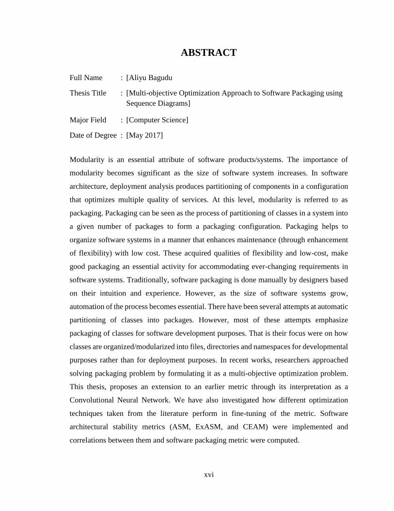
ABSTRACT
Full Name : [Aliyu Bagudu
Thesis Title : [Multi-objective Optimization Approach to Software Packaging using
Sequence Diagrams]
Major Field : [Computer Science]
Date of Degree : [May 2017]
Modularity is an essential attribute of software products/systems. The importance of
modularity becomes significant as the size of software system increases. In software
architecture, deployment analysis produces partitioning of components in a configuration
that optimizes multiple quality of services. At this level, modularity is referred to as
packaging. Packaging can be seen as the process of partitioning of classes in a system into
a given number of packages to form a packaging configuration. Packaging helps to
organize software systems in a manner that enhances maintenance (through enhancement
of flexibility) with low cost. These acquired qualities of flexibility and low-cost, make
good packaging an essential activity for accommodating ever-changing requirements in
software systems. Traditionally, software packaging is done manually by designers based
on their intuition and experience. However, as the size of software systems grow,
automation of the process becomes essential. There have been several attempts at automatic
partitioning of classes into packages. However, most of these attempts emphasize
packaging of classes for software development purposes. That is their focus were on how
classes are organized/modularized into files, directories and namespaces for developmental
purposes rather than for deployment purposes. In recent works, researchers approached
solving packaging problem by formulating it as a multi-objective optimization problem.
This thesis, proposes an extension to an earlier metric through its interpretation as a
Convolutional Neural Network. We have also investigated how different optimization
techniques taken from the literature perform in fine-tuning of the metric. Software
architectural stability metrics (ASM, ExASM, and CEAM) were implemented and
correlations between them and software packaging metric were computed.

xvii
ملخص الرسالة
:الاسم الكامل
نهج متعدد الأغراض الأمثل لبرامج التعبئة والتغليف باستخدام تسلسل الرسوم البيانية :عنوان الرسالة
علوم الكمبيوتر التخصص:
1438شعبان : :العلميةتاريخ الدرجة
.البرمجيات نظام حجم زيادة مع كبيرة تصبح النمطية أهمية .البرمجيات أنظمة /منتجات من أساسية سمة هي النمطية
هذا في .المتعددة الخدمات جودة من يحسن تكوين في المكونات تقسيم النشر تحليل ينتج البرمجيات، هندسة وفي
إلى نظام في الطبقات تقسيم عملية والتغليف التعبئة اعتبار ويمكن .والتغليف التعبئة كما نمطية إلى ويشار المستوى،
بطريقة البرمجيات أنظمة تنظيم على يساعد والتغليف التعبئة .والتغليف التعبئة تكوين لتشكيل الحزم من معين عدد
التكلفة، ومنخفضة المرونة من المكتسبة الصفات هذه .التكلفة انخفاض مع (المرونة تعزيز خلال من )الصيانة تعزز
يتم تقليديا، .البرمجيات أنظمة في باستمرار المتغيرة الاحتياجات لتلبية أساسيا نشاطا جيدة والتغليف التعبئة وجعل
العملية أتمتة تنمو، البرمجيات نظم حجم مع ذلك، ومع .والخبرة الحدس أساس على المصممين قبل من يدويا التغليف
تؤكد المحاولات هذه معظم فإن ذلك، ومع .حزم إلى للفصول تلقائي لتقسيم محاولات عدة هناك كانت .أساسيا يصبح
الملفات في نمطية /الطبقات تنظيم كيفية على تركيزهم هو وهذا .البرمجيات تطوير لأغراض للفئات والتغليف التعبئة
حل من الباحثون اقترب حديثة، أعمال في .النشر لأغراض من بدلا التنمية لأغراض الأسماء ومساحات والدلائل
مقياس إلى تمديدا تقترح الأطروحة، هذه .الأهداف متعددة الأمثل كمشكلة صياغته خلال من والتغليف التعبئة لمشكلة
المختلفة التحسين تقنيات أداء كيفية في بالتحقيق أيضا قمنا لقد .التلافيفية العصبية شبكة باعتباره تفسيره خلال من سابق
وتم ،(إكسسم )للبرامج جديد معماري استقرار مقياس صياغة أيضا تم وقد .المقياس صقل في الأدبيات من المأخوذة
البرمج التعبئة مقياس صحة من للتحقق لاستخدامه محاولة إجراء
1
1 CHAPTER 1
INTRODUCTION
1.1 Motivation
Software packaging is the process of partitioning or clustering of all class modules in a
software system into a set of clusters/packages for developmental or deployment purposes.
In software architecture, a package can be viewed as a component. Components are
independent executable units that interact with each other. Components are composition of
classes and/or other components [44]. This type of packaging process is referred to as
deployment analysis in software architecture.
A packaging configuration is an instance of the set of all possible outputs the packaging
process can produce. The term packaging also refers to a packaging configuration. Here
we assume that packages in a configuration are nonintersecting sets of classes. This implies
that a configuration cannot have more than one instance of a class and equivalently a class
cannot be present in more than a single package. Thus the highest number of packages we
can have in a packaging is equal to the number of classes in the entire system. That is each
class being treated as a package. While on the other extreme case we may have a single
package with all the classes.
Packaging for software development purposes has its own benefits such as maintainability,
and reusability. Moreover, what is important and of interest to software architecture is the
2
deployment architecture [44]. The deployment architecture is an arrangement of
components of the system in a certain manner for deployment purposes. This has a
significant impact on the quality of service (QoS) of the system. The QoS here does not
only pertain to the development but most importantly to the use of the system.
In large commercial software systems, composed of many components providing different
services, it is desired that the classes are packaged into components based on the services
they provide and the intercommunication between them. A general aim is to increase
cohesion among classes in the same package and to reduce coupling between packages.
Having class modules that provide a single service composed in a single package is
intuitive because it will be more efficient in terms of user-interaction response and
minimization of latency. Additionally, when a service fails other parts of the system will
still function providing services. Maintenance of the system can also be performed on a
module without having much impact on the entire system. Based on this intuition, we can
decide class modules that should be together in the same package.
However, how to select which class modules to put together may not be straightforward
especially in the case of large systems. A single class may be communicating with multiple
other classes that are involved in different services or scenarios. That is a single class may
be involved in more than a single scenario. Therefore, if decision is made to group packages
by services/scenario they partake in, a manual packaging will be almost impossible if the
system is too large
Hence, a more systematic approach that can automatically suggest good packaging
configurations is essential. In software packaging, there are several competing goals we
3
want to achieve. If minimizing coupling and maximization of cohesion are our only
objectives, we may decide to put all class modules in a single package. However, if we are
considering just modularity, we will seek to package the classes in a manner whereby class
modules participating in a single scenario and that scenario only, are placed together in a
package. However, we want to achieve multiple quality objectives that are conflicting at
the same time.
Two major challenges facing effective packaging are: lack of effective metric to quantify
the packaging objectives; and large search space to search through for the optimal
packaging combination. The latter is termed as combinatory optimization problem [20].
This multi-objective goal coupled with the large search space in which to search for optimal
packaging solution, justifies employment of randomized and evolutionary optimization
algorithms. Generally, modularity helps in managing complexity; it encourages
simultaneous development of different modules; and it better copes with uncertainties [1].
1.2 Problem Statement
Software packaging problem is a hard problem to solve [20][4].
To tackle the difficulty associated with the definition and quantification of quality of a
software packaging, metrics have been proposed and hypothesized. The literature review
section discusses earlier works.
However, the research gap here is that these proposed metrics need further validation. This
problem of further validation applies to many proposed software metrics. That is why these
works [23][57][34] are all about further validation of software metrics – either through
correlation check with some other more reliable metrics or by other means.

4
Moreover, a further new techniques for formulation of software packaging quality metrics
can also be investigated.
The goals of this thesis are denoted as follows:
Goal 1: Extension of an earlier metric.
Investigation and reproduction of the earlier metric by Ebad and Ahmed [20] and to extent
its functionality.
Goal 2: Investigation of the effectiveness of optimization techniques.
The second goal of this thesis is to investigate whether other optimization techniques from
the literature will perform better in this optimization problem.
Some of the potential optimization algorithms to investigate are Differential Evolution
(DE) [58], Ant Colony (AC) [15], Particle Swarm (PS) [29], Genetic Algorithm (GA) [47],
and Covariance Matrix Adaptation- Evolution Strategy (Cma-es) [11].
Goal 3: Investigation correlation between packaging metric and stability metric
To check if there is correlation between software packaging metric and software stability
metric. This is to enable us make an intuitive sense of a correlation between software
packaging quality and software stability.
1.3 Research Hypotheses
The research hypotheses are denoted as follows:
Hypothesis 1: The metric used by Ebad and Ahmed [20] can be reinterpreted and
extended to make a better software packaging metric.
5
Hypothesis 2: Other optimization techniques will perform better than those
employed earlier by [20].
Hypothesis 3: There is a correlation between the software packaging metric and the
stability metric.
1.4 Thesis Approach
Convolutional Neural network approach was used to interpret the earlier metric and that
provided a way to extend it.
Experiment was conducted to compare optimization algorithms. Meta-heuristic
optimization algorithms approach were used. Five trial runs of given combination of
selected parameters of the algorithms were recorded. The average of the best score of each
trial runs was computed and used to compare the algorithms.
Architectural stability metrics (ASM, ExASM, CEAM) were implemented and were used
to check if there exists a correlation between the packaging metric and stability metric.
Nine cases of changes to the hypothetical case study were considered. Further four different
scenarios of changes to the case study were considered.
Empirical approach was employed in all studies. Real and hypothetical case studies were
employed in the empirical studies.
1.5 Thesis Contributions
This thesis offers the following main contributions:
Contribution 1:
6
An interpretation of the metric as convolutional neural network was developed. It was
shown how the metric can be extended through that interpretation. This paves way for
investigating how many other software metrics can be interpreted and extended through
neural network.
Contribution 2:
Several stability metrics (ASM, ExASM and CEAM) were implemented and there
correlation with software packaging metric was investigated. A correlation between
software packaging metric and CEAM metric was confirmed through the experimental case
studies.
Contribution 3:
Steps to be taken to identifying, analyzing, formulating and solving an optimization (multi
or single objective) problem were outlined. This will serve as a guide for researcher
pursuing this endeavor.
I have shown clearly the relationship between machine learning and optimization. Helping
new and novice researchers understand what they mean and how they relate.
Therefore, others trying to solve any optimization problem will gain some useful insight
from this work.
1.6 Thesis Outline
The remaining parts of the thesis are divided into five chapters:
Chapter 2 gives background about multi-objective optimization problem and how they are
solved. Learning and validation process was also explained. Meta-heuristic optimization

7
algorithms approach was described. Chapter 2 also reviews and discusses earlier work
that has been done on software packaging metric. Methodology adopted to solving the
different problems related to the research objectives are discussed in chapter 3. Results of
the investigations are reported and analyzed in chapter 4. Conclusions were made in
chapter 5 based on the results.
8
2 CHAPTER 2
BACKGROUND
2.1 Multi-objective optimization
In computer science, problems can be classified either as decision or optimization problem
[4][45]. Decision problems are the ones with yes or no output solution when given an input
instance [64]. Optimization problems involve outputting a solution that either minimizes
or maximizes a quantity when given an instance of a problem[45]. All optimization
problems have corresponding decision problem component that has to be solved severally
in the course of solving the optimization problem [52].
However for the purpose of classifying problems based on asymptotic run time complexity,
only decision problems are considered because an optimization problem falls in same
complexity class as their corresponding decision problem [12]. That is if a decision
problem that is a component of an optimization problem is in given class, then the
optimization problem also fall into the same class [12][4].
In classification of problems based on their asymptotic run time complexity, a problem is
considered to be in class P if there exist a deterministic algorithm to solve the problem in
polynomial run time [4]. A problem is considered to be in class NP, if there exist a
nondeterministic algorithm to solve the problem in polynomial run time complexity [4].
There are also other classes such as NP-Hard and NP-Complete [4].
9
The NP problems (excluding P class) are deemed to be more difficult to solve and have no
polynomial time deterministic algorithm to solve them [4]. Moreover most of the practical
problems in real life fall in this category [14]. The packaging problem in this work also
falls in this category [20].
Optimization problems can be seen as a search problem involving a search for a solution
that optimizes an objective value or multiple objective values [52]. The solution can be of
one or more dimension depending on the number of variables it has. The number and type
of variables - the number and type of values of variables - determine the scope of the search
or solution space [52]. A solution is normally referred to as a point, candidate, or an
individual. It can be a point or set of points [40].
2.1.1 Solution space
To understand how optimization problems are solved, one needs to understand the idea of
solution space. The space where all the solutions of the problems are based. The way a
solution to the problem is found is also dependent on the nature of the solution space. This
can be seen as a space of a given number of dimensions as the number of variables. There
are usually additional predicates that further restricts the points in the solution space. This
predicates can be in the form of constraints or bounds. The nature of the space is dependent
on the types of variables that make up the space [52]. This space can be imagined as are
Cartesian coordinate.
A constraint is a predicate that comprises of a function of the points of the space whose
output is related to a value or set of values by an equality relation. Bound predicates are
same as constraints predicates however they have inequality relation instead. Both types of
10
predicates further constrains the points of the solution space to a limited set of points. The
term constraint is simply used to refer to both types of predicates [9].
Worth noting is that the variable type of the objective function is distinguishable from
variable types of dimension of points in the solution space.
2.1.2 Variable types
quantitative (orderable):
o continuous: (differentiable or non-differentiable )
o discrete: integer
qualitative: (categorical)
Quantitative variable are those which have ordering among all of its possible values [24].
They are those variable types for which it is valid to compare a pair of it values by an
inequality relation. That is it can be said that a value is less, equal, or greater than another.
Variable types of the objective function has to be orderable to be an optimization problem
involving minimization or maximization. When the objective function output variables are
not orderable, then the problem becomes mixed variable programming (MVP)
[31][10][37] that involves searching for a pattern from the solution space. There can be
continuous objective function output only if all the variables of the points are continuous
[59].
Continuous variable is one whose values span the space of real numbers [33]. They give
rise to a differentiable or non-differentiable functions. Differentiability of function matters
in the realms optimization because some optimization techniques make use of it to compute
the direction of slope [32]. Also for derivative based techniques to be used the objective

11
function has to be a white-box function whose derivative is computable [32]. In this
packaging optimization, the objective is treated as black-box function [20].
Discrete and categorical variables are similar however categorical variable are not
orderable while discrete variables are. Caution must be taken when dealing with categorical
variable that have discrete labeling because often numbers are used to label articles without
necessarily implying any order. The type optimization that deals with only discrete
candidate solution is what is called integer programming [49]. While those that involves
categorical variables are called combinatorial optimization [50]. Thus, the packaging
problem we have is a combinatorial optimization problem [20].
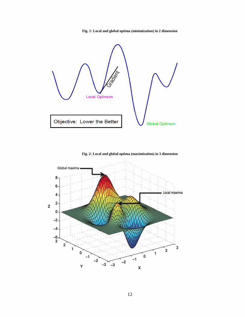
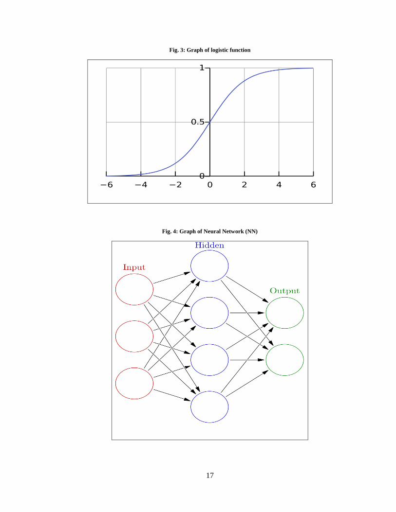
2.1.3 Local and global optimum
Local optimum is a point that has the best value among its immediate neighbors in all
directions. Global optimum is the best point among all the local optimums. Most of the
optimization algorithms use slope testing techniques to converge to the optimum solution
point(s). However, all optimums either local or global have same slope behavior and so
there is no way to distinguish the global optimum from other optimum points. Thus, the
presence of many local optima, is what actually makes optimization difficult to sovle [63].
Fig. 1 and Fig. 2 illustrates the idea of local and global optima. Fig. 1 has solution space in
1 dimension along the horizontal axis and the objective functionoutput indicated along the
vertical axis. Fig. 1 is a minimization problem. Fig. 2 has solution space in 2 dimensions
along X and Y axis, and the objective function output indicated along the Z axis. Fig. 2 is
a maximization problem.
12
Fig. 1: Local and global optima (minimization) in 2 dimension
Fig. 2: Local and global optima (maximization) in 3 dimension

13
2.1.4 Coping with problem hardness
As discussed earlier, there are problems that are hard to solve and have an exponential run
time when solved with deterministic algorithms. To cope with those problems, are there
techniques used to produce an optimal or near optimal solution that may be appreciable.
The solution produced by these techniques may be guaranteed to be within a difference
bound of the optimal, or a ratio bound of it [4]. Moreover we may be also able to talk about
the properties of the produced solution such as probability of producing the correct answer
and the expected run time [4].
Backtracking technique is employed to design an algorithm to solve hard problems when
it is desired to obtain an optimal solution from the algorithm. So what this technique does
is to use systematic techniques for searching with the hope of cutting down the search space
[4].
Approximation algorithms use intuitive heuristics to produce an approximate optimal
solution or if lucky the optimal solution to the problem. Randomized algorithm introduce
random input(s) in order to guess solutions and thus reduce runtime of producing the
solution [4].
Meta-heuristic algorithms are more of general optimization algorithms that are not problem
specific. They employ both random input(s) and generic heuristics to solve problems [30].
They are those employed in and one of the focus of this research work. Meta-heuristics
algorithms mostly draw their inspiration from the nature [28]. Mimicking how nature
solves hard problems. A class of meta-heuristic algorithms is evolutionary optimization
algorithms [56][40] (population based) that uses mechanisms inspired by biological

14
evolution, such as selection, reproduction, mutation, and crossover among population of
candidate solutions [48]. They use a population of candidate solutions rather than just
iterating over one point in the search space. On the other hand are single candidate meta-
heuristic optimization algorithms that evolves through iteration over a single candidate.
These single candidates are also normally inspired by natural process such as simulated
annealing [61] based on the principle of cooling of molten metal.
2.1.5 Single and Multiple objective functions
In optimization problem there can be more than a single objective function [65]. These
objectives may even be conflicting with each in the sense that changing the value of a
variable of a solution point may lead to an increase and the other decreasing [6]. However
contradicting objectives are not actually the main problem because any of the objectives
can easily be negated to make them all have a single objective (either minimization or
maximization) [17].
There are different approaches for solving multi-objective optimization problems
(Aggregating, Population-based non-Pareto, Pareto-based non-elitist, Pareto-based elitist
approaches) [6] . The scope of this work is Weighted sum Aggregating approaches [6].
The problem however, is how should these objectives be combined to form a single global
objective function in an aggregating approach manner? The truth is we do not actually
know exactly how to until we have some more information about the relation between the
objective functions. This relationship implies how the objectives are combined to formulate
the global objective function. To find the global optimum one has to find all the local
optimums and then compare them.

15
An objective function is a function of input variables of the solution space the same way
the global objective function is a function of each objective functions that combine to form
it. Thus, we can look at variables as objective functions in single objective function and in
the same way objective functions as variables in multiple objective function.
The simplest combination will be assuming that all objective functions have equal weight
and could then be added to formulate the global objective function. This simple idea can
be further extended by further assuming that the objective functions have different weights
that signifies what percentage they contribute to the global objective function. This way,
each objective function is multiplied by a respective weight parameter and the products are
added to formulate the global objective. Another very important question to keep in mind
is how do we know the weight of those parameters [22]? This simple way of formulating
the objective function can be termed as a linear regression (linear combination) objective
function. Higher polynomial terms and their respective weights can also be added to
objective function to form polynomial regression. Thus we can have objective function
formulated as logistic function in logistic regression and so on.
• We can consider objectives as variables x1, x2, …, xn
• We have several ways of combining multiple objectives into a single one x.
• Make all objective have single direction: either all minimization or all
maximization by multiplying by -1 where needed
• It could be as simple as linear combination [6]:
▫ x = x1 + x2 + … + xn = xv

16
▫ linear(xv)
• weighted linear combination [6][22]
▫ x = w0 + w1*x1 + w2*x2 + …+ wn*xn = xvTwv
▫ weightedLinear(xvTwv)
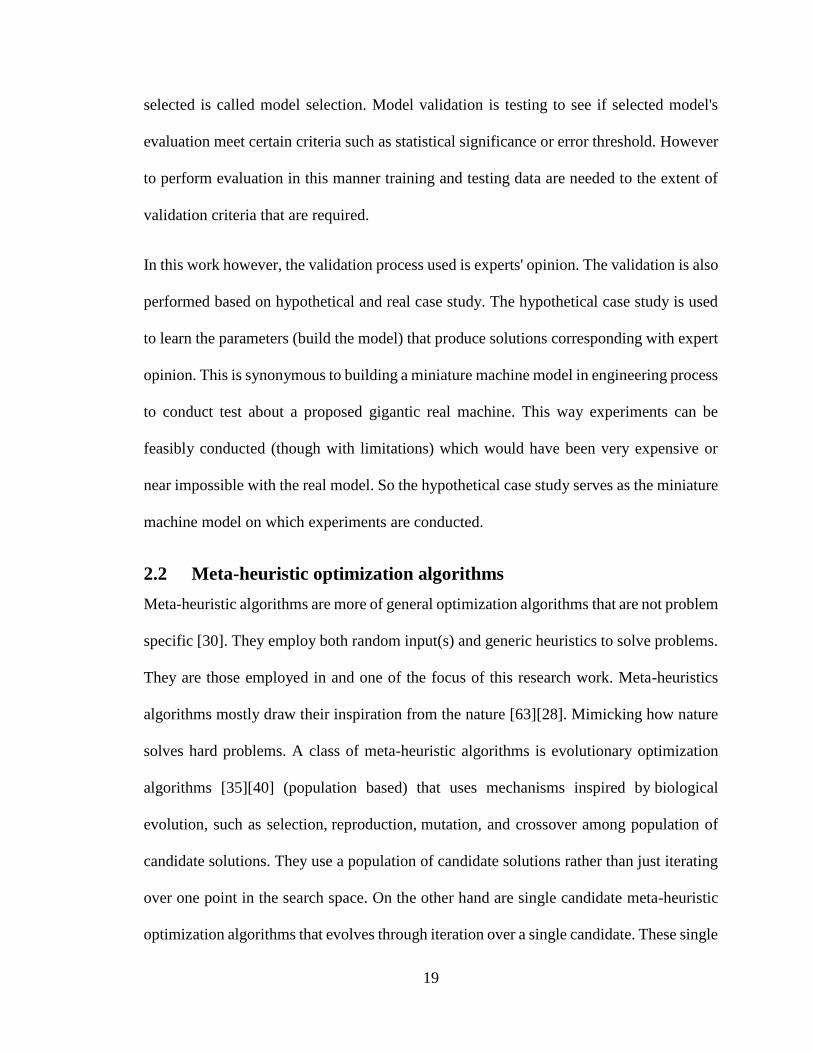
• Or more complex such as:
• Logistic (linear, normalized) [36]
▫ x = 1/[1 + exp - (w0 + w1*x1 + w2*x2 + …+ wn*xn )]
▫ logistic(xvTwv)
• Radial basis regression(nonlinear) [62]
▫ x = exp[-(xv - cv)/2r2]
▫ localweight(xv ,cv,r2)
• Polynomial regression(nonlinear ) [25][54]
▫ Polynomial interpolation
▫ x = (xvTwv + c)d
▫ Polynomial(xv ,wv , c , d)
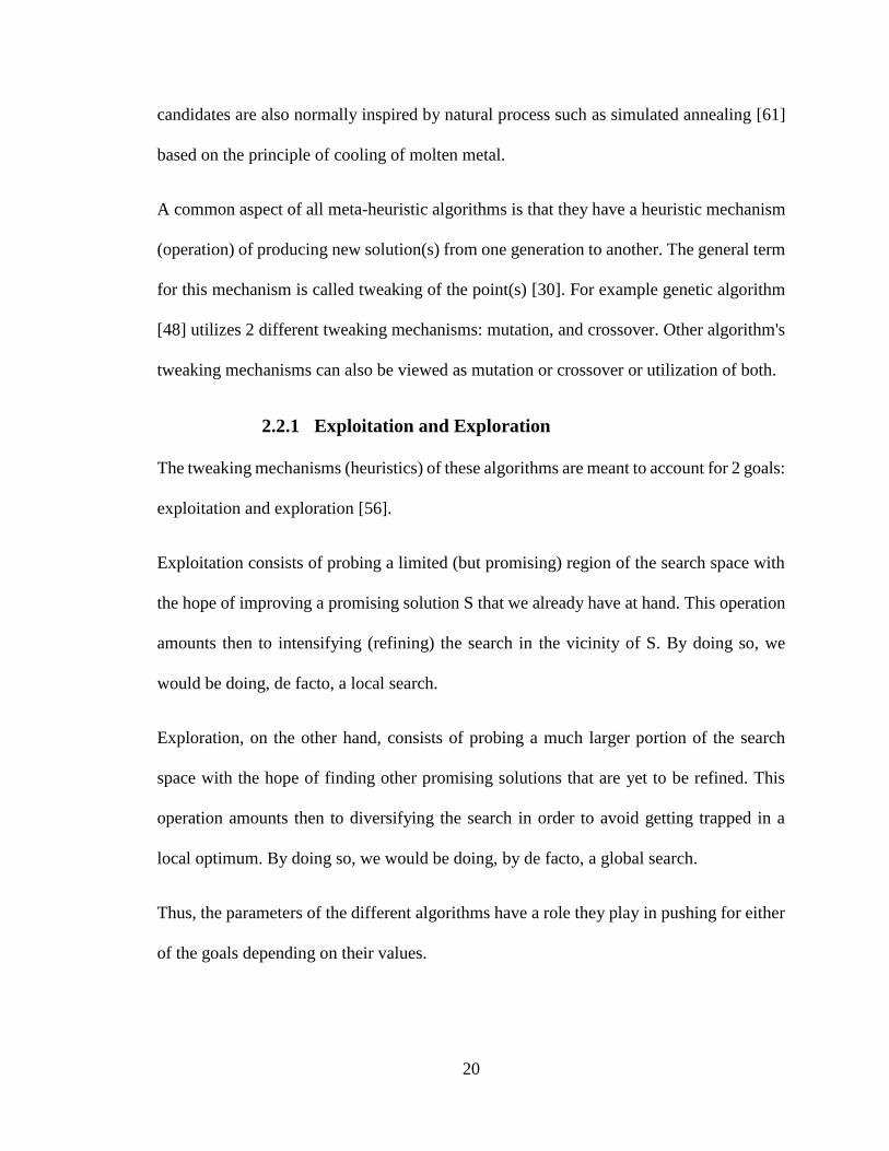
• A neural network (nonlinear, normalized) [53][26]
▫ Where each unit is logistic or sigmoid function
17
Fig. 3: Graph of logistic function
Fig. 4: Graph of Neural Network (NN)

18
However, we still have those questions that arise such as which type of objective function
[6] is suitable or what the value of the parameters [22] should be? The answer is: we don't
know and an investigation is necessary. It then becomes a statistical learning problem
where we learn what parameters best suits the problem. It can also be called a machine
learning problem. However, in a learning process examples are required to be used to learn
the best possible value of the parameters. An objective function formulation with all its
parameters is called a (statistical) model. This is also called a family of objective functions
where for each unique combination of values of the parameters we have a member of the
family. The process of learning the values of the parameters is known training the model.
However, in many context, getting a sufficient (significant) number of examples to train a
model is challenging because they are difficult to acquire and encode. In this cases
assumptions are made.
Moreover, there is principle of Occam's razor that states that among competing hypotheses,
the one with the fewest assumptions should be selected. This can be put in another way
that the simplest assumption is the best assumption in the absence of evidence or more
evidence. That we should not complicate matters beyond necessity. By this principle it is
always good to assume a linear combination objective function. Linearity is intuitive and
easily assimilated by human reasoning.
2.1.6 Model evaluation and selection
Model evaluation is process of measuring how well a model represent the true system.
Generalization error computed using cross-validation technique is used in model
evaluation. The process where the model that produces the least generalization error is
19
selected is called model selection. Model validation is testing to see if selected model's
evaluation meet certain criteria such as statistical significance or error threshold. However
to perform evaluation in this manner training and testing data are needed to the extent of
validation criteria that are required.
In this work however, the validation process used is experts' opinion. The validation is also
performed based on hypothetical and real case study. The hypothetical case study is used
to learn the parameters (build the model) that produce solutions corresponding with expert
opinion. This is synonymous to building a miniature machine model in engineering process
to conduct test about a proposed gigantic real machine. This way experiments can be
feasibly conducted (though with limitations) which would have been very expensive or
near impossible with the real model. So the hypothetical case study serves as the miniature
machine model on which experiments are conducted.
2.2 Meta-heuristic optimization algorithms
Meta-heuristic algorithms are more of general optimization algorithms that are not problem
specific [30]. They employ both random input(s) and generic heuristics to solve problems.
They are those employed in and one of the focus of this research work. Meta-heuristics
algorithms mostly draw their inspiration from the nature [63][28]. Mimicking how nature
solves hard problems. A class of meta-heuristic algorithms is evolutionary optimization
algorithms [35][40] (population based) that uses mechanisms inspired by biological
evolution, such as selection, reproduction, mutation, and crossover among population of
candidate solutions. They use a population of candidate solutions rather than just iterating
over one point in the search space. On the other hand are single candidate meta-heuristic
optimization algorithms that evolves through iteration over a single candidate. These single
20
candidates are also normally inspired by natural process such as simulated annealing [61]
based on the principle of cooling of molten metal.
A common aspect of all meta-heuristic algorithms is that they have a heuristic mechanism
(operation) of producing new solution(s) from one generation to another. The general term
for this mechanism is called tweaking of the point(s) [30]. For example genetic algorithm
[48] utilizes 2 different tweaking mechanisms: mutation, and crossover. Other algorithm's
tweaking mechanisms can also be viewed as mutation or crossover or utilization of both.
2.2.1 Exploitation and Exploration
The tweaking mechanisms (heuristics) of these algorithms are meant to account for 2 goals:
exploitation and exploration [56].
Exploitation consists of probing a limited (but promising) region of the search space with
the hope of improving a promising solution S that we already have at hand. This operation
amounts then to intensifying (refining) the search in the vicinity of S. By doing so, we
would be doing, de facto, a local search.
Exploration, on the other hand, consists of probing a much larger portion of the search
space with the hope of finding other promising solutions that are yet to be refined. This
operation amounts then to diversifying the search in order to avoid getting trapped in a
local optimum. By doing so, we would be doing, by de facto, a global search.
Thus, the parameters of the different algorithms have a role they play in pushing for either
of the goals depending on their values.
21
2.2.2 Genetic algorithm (GA)
Genetic algorithm (GA) is a population based optimization technique. It is inspired by
natural evolutionary process theory of selection – survival for the fittest. In this
optimization process the fittest members of the population have the highest chance of
producing the next generation. A solution is regarded as an individual competing among
other individuals in a population. In the natural evolution process, kind of individuals for
subsequent generations depends on the natural operations such as crossover, inheritance,
mutation and selection [48].
Genetic algorithm can be seen as a framework for many evolutionary optimization
algorithms where the heuristics of an algorithm can be made analogous to one of the stages
or operations of genetic algorithm. With this view, other algorithms can be integrated into
MATLAB GA toolbox to harness the features of the toolbox such as algorithm data
collection and visualization.
2.2.3 Covariance matrix adaptation-evolution strategy (CMA-
ES)
The CMA-ES (Covariance Matrix Adaptation Evolution Strategy) is an evolutionary
algorithm that uses adapted covariance matrix to define a n-sphere around the specified
feasible region range [11]. It is used for highly non-linear, non-convex, and black-box
optimization problems [11]. CMAE-ES is regarded as a state-of-the-art optimization
algorithm because of it use as a standard optimization tool across the industries [11]
22
2.2.4 Particle swarm optimization (PSO)
As with many other optimization algorithms, particle swarm optimization (PSO) is an
optimization algorithm (OA) that mimics biological animal behavior. In particular, PSO
mimics optimal behavior of swarm birds (particles) in search of food (solution).
PSO uses simple mathematical formula to calculate and track the position and velocity of
each particle [29].
Further details on the working of PSO can be found in [51] where some theoretical
convergence conditions were also discussed.
2.2.5 Differential evolution (DE)
An important aspect of global optimization using meta-heuristics is the generation of initial
population especially for the population-based heuristic optimization methods. Differential
Evolution is a relatively recent population-based search heuristic used by engineers to solve
continuous optimization problems. It does not only use simple evolutionary strategy but
also functions significantly faster and in robust manner when it comes to solving
optimization problems, hence high likelihood to find the global optimum. It has a wide
acceptability due to the fact that it has a very few number of parameters and has a compact
structure with a small code. Most of the studies have been proposed in order to improve
the performance of DE. A number of the studies employ tuning or controlling the
parameters of the algorithm and improving the mutation, crossover and selection
mechanism [58] [2].

23
2.2.6 Performance assessment
There several factors that could be used to assess the performance of the algorithms. Some
of this factors have an associated graphical plot that could be used to visualize them. The
data pertaining to these factors are collected at each generation (iteration). Fig. 5 shows the
visualization of some these factors. This visualization depicts GA with 7 dimensional data
points, with population size of 20, and made about 90 iterations. Below is a list of factors
and their descriptions used to evaluate the algorithms.
Fig. 5: OA performance visualization
Best fitness plots with black dots the best function value against generation and in
the blue dots is plot of average function value of individuals in a generation versus
generation. It is used to monitor whether the algorithm's "best value ever" is only
getting better as it makes progress. The average score per generation gives a feel of
whether the algorithm's population converges as it progresses and thus giving a feel

24
of exploitation. Caveat here is we may try to use this to get a feel of exploration at
the end if the average fitness value does not equal best fitness value. The average
fitness could may best fitness value in case where all optimum solutions discovered
have same value. This may even be more likely where multiple solution
representations (genotype) could refer to a single solution. In addition different
solution points could have same score. We could also get a feel of whether the
algorithm is merely a random process throwing random points around in which case
the average fitness value will show a constant trend.
Best individual plots the vector entries of the individual with the best fitness
function value in each generation. Therefore, what the graph currently shows is the
best individual the last generation.
Average Distance plots the average distance between individuals at each
generation. This enables us to visualize how wide spread the individuals in the
population are. This will enable us know whether the algorithm balances between
exploration and exploitation. if for instance the average distance is zero at a given
generation, that means all the population members have converge to a solution
point. We may want the average distance to show a decreasing trend to give us a
sense of convergence and thus exploitation. However, we may not want the average
distance to converge to zero in order to guarantee that even at the last generation
the solution points are apart to ensure that exploration has taken place.
Expectation plots the expected number of children versus the raw scores at each
generation.
25
Scores plots the scores of the individuals at each generation. This enables us to
visualize scores of all individuals to get a sense of diversity among the population
which implies exploration. What the graph currently shows are the individual
scores at the last generation. If the number of individuals is large then Score
diversity plots can be used instead to plot a histogram of the scores at each
generation.
Selection plots a histogram of the parents. This show the individuals in the current
generation and their likelihood of being selected has parents to produce the next
generation. What the graph currently shows are the likelihood of individuals at the
last generation. This can be useful if we are interested in monitoring exploration to
see if the algorithm gives any chances at all for individual with low score.
2.2.7 Parameters types
There are three types of parameters involved in optimization experiments. First, is model
parameter - for example the weight of parameters discussed earlier. They are later used in
prediction with the model. Second, it is hyper-parameter that helps to choose a model from
a complex super-set model. They may also be used in prediction with the model if no effort
is made to identify the model selected from the super-set model. Third is algorithm
parameter which also helps choose a model but is specific to an algorithm and only used
in the optimization process. They don't appear when the model is used for prediction.
However, both hyper-parameter and algorithm parameter can be simply referred to as
hyper-parameter (or meta-parameter). Moreover, we are dealing only with model and
algorithm parameter in our case.
26
2.2.8 Parameter Search Techniques
Search grid is a manual parameter search technique which discretizes the values of all
factors involved in an experiment to specific respective set of values, and evaluate all
combinations of factor values so that the best parameters' values combination that produces
the best fitness can be identify.
Hyper-parameter optimization is broader term for techniques used in fine tuning of hyper-
parameters and algorithm parameters to select an optimization model. The other type of
hyper-parameter tuning technique is meta-optimization, where the parameter search
problem is also formulated as an optimization problem to obtain value(s) of parameter(s)
that correspond to local optima. That is you have an optimization problem inside another
which is being used to fine tune its parameters.
2.3 Literature Review
2.3.1 Packaging quality metric
Many approaches have been proposed in the literature that attempt to apply different
methods and algorithms in order to achieve design modularization for the components of
software systems.
Mancoridis et al. [42] [41] developed a special tool, called Bunch. It uses hill climbing and
genetic algorithm for optimizing their clustering objective function. The system is based
on the relationship between entities in the source code. The modularization quality (MQ)
that is calculated as trade-off between the intra-module and inter-module connectivity, was
used as objective function. For representation of the system, they calculated the MQ by
subtracting the average inter-connectivity and the average intra-connectivity. They used a
27
module dependency graph (MDG) that is built based on the components of the system and
relationships that exist in the source code.
Liu et al. [35] attempts to solve problem of minimization of traffic across computer network
involving multiple servers and users by formulating the multi-objective problem as
partition of users into a number of nonintersecting sets equal to the number of severs. The
approach tries to optimization such that within-partition dependencies are high and
between-partition dependencies are low. They used Grouping Genetic Algorithm (GGA)
that is used for large -scale partitioning problem. Their ultimate aim was to minimize
network traffic in the entire network.
Bauer and Trifu [8] presented a way to produce a packaging by combining clustering with
pattern recognition algorithms to recover subsystems similar to what software engineers
achieved by reverse engineering.
Using the Bunch tool, Doval et al. [16] employed GA algorithm to seek an optimal
grouping using modularization quality objective function. They used roulette wheel
selection while standard mutation and crossover were used. The used crossover rate of 80%
for populations of 100 individuals and 100% of a 1000 individuals. The mutation rate used
is 0.0004log (N). Where N is the number of nodes in the MDG.
Mitchell and Mancoridis [46] extended the Bunch tool by addressing a shortcoming that
makes it produce clusters that minimize the inter-edges exiting in clusters rather than
minimizing the total number of inter-edges all together. Thus, they came up with a
modification of MQ and integrated it into the tool. The new MQ supports MDGs with edge
weights, while the original MQ measurement did not.
28
Seng et al. [55] used a combination of software metrics and design heuristics to formulate
a function to calculate the quality of subsystem decomposition. They also used group
genetic algorithm (GGA) as the main algorithm applied in this situation with the fitness
function being a multi-objective function that accounts for cohesion, complexity, coupling,
cycles, and bottlenecks.
Alkhalid et al. [3] proposed an approach on the package level. They used the refactoring
approach, and they classified the classes in two approaches: An approach where number of
packages are fixed; and an approach where number of packages is variable. They applied
different clustering approaches whose results were compared with those of two software
engineering experts/faculty to validate their results. A similarity measure proposed by
Lung et al. [38] was used in their packaging approach.
Abdeen et al. [1] proposed an approach to enhance the existing modularization by
minimizing the inter-package connectivity. They did several experiments and they
described the dependency quality as a weighted average of the common closure quality and
acyclic dependency quality. Compared with the previous methods, their approach makes
provision for setting constrains such as the size of the package, modularization structure,
etc.
Earlier works such as Ebad and Ahmed [20] emphasized packaging of classes for
developmental purposes. Their focus was on how classes are organized/modularized into
files, directories and namespaces for developmental purposes rather than for deployment
purpose. In partitioning of modular systems, partitioning based on functional aspects was
emphasized [20]. Moreover, prior to their approach all attempts at automatic packaging
29
were not function driven. This led Ebad and Ahmed [20] to embark on the course
functionality based software packaging. Ebad and Ahmed [20] validated there approach
using three means: first is validation against theoretical properties of good metrics; second
is an experiment on hypothetical case study; and third is an experiment of on real-case
study.
Ebad and Ahmed [20] proposed a metric to separate the classes of class diagrams into
packages in the architecture design phase. They presented this method to address
modularization. They showed that by allowing each package to offer a single function and
that function being completely executed within that package, we can achieve a cohesive
modularization. They validated the metric against the theoretical properties and they
applied it to two search techniques: exhaustive search approach; and heuristic search
approach. They also applied their approach to two case studies whose outcomes were
encouraging.
They formulated a multi-objective packaging metric on which they employed three
optimization algorithms - Simulated Annealing (SA), GGA-Evolver Genetic Algorithm
(GA) and Hill Climbing (HC). However, the shortcoming with their approach is that
packaging configuration with all the classes in one package is scored highest by the metric
at the expense of desirable feasible configurations that gives realistic number of packages.
In this case if the number of solutions the optimization algorithm (i.e. GA) is required to
produce is few then realistic solution may even not be present because the GA is supposed
to produce the fittest possible individuals it can produce. Moreover, if the optimization
algorithm is required to produce too many solutions then, it will consume much time and
30
manual selection still has to be done on the many solutions produced to choose a realistic
solution.
The packaging metric [20] was referenced by Ebad [18] in his work on measuring software
requirement volatility. This reference is made as a result of use of same JHotDraw software
as case study and the use of use of similar theoretical validation approach. The packaging
metric was also referenced in another work by Ebad [21] where they reviewed and
evaluated cohesion and coupling metrics at packaging and subsystem level.
2.3.2 Architectural stability metrics
Jazayeri [27] used a retrospective approach to assess software architectural stability where
20 releases of a telecommunication software was used as a case study. A metric was not
formulated in this work however 3 analysis approach were employed in the assessment –
simple metric analysis, Hidden module coupling, and Color visualization. The simple
metrics were all based on size of system and they include number of programs, number of
added programs, percentage of added and changed programs, and size of modules. The
hidden module coupling simply involves physically examining which programs always
change together in each releases to ascertain if the is certain relationship between them. In
color visualization, color percentage bars were used to display a history of a release.
Aversano et al. [5] work was based on investigating stability of software projects through
software project life cycle with the aim of ascertaining software components that are stable
enough to be reused in other projects. They defined Core Design Instability (CDI) and Core
Calls Instability (CCI) metrics. The metrics were based on architectural core - which is
31
regarded as the packages that are involved in 80% of inter-package communications.
Where CDI accounted for number of packages, CCI accounted for number of inter-package
calls. Both CDI and CCI were defined in the same manner as ASM. To simply put it ASM
as same idea as CCI but in ASM all packages are used instead of the so called cores. Real
software projects from SourceForge were used as case studies in the work.
In the work done by Bansiya [7], a metric called extent-of-change (EoC) was proposed as
a measure of software framework architectural stability. The properties used to calculate
EoC are Number of Classes, Number of Hierarchies, Number of Single Inheritances,
Number of Multiple Inheritances, Average Depth of Inheritance, Average Width of
Inheritance, Number of Services, Number of Parents, and Direct Class Coupling. The main
difference between this approach and ASM is that this approach is at class level. This
methodology was applied to the Microsoft Foundation Classes (MFC) and Borland Object
Windows (OWL) application framework systems to compute the structural characteristics
and thus the extent-of-change in several releases of the frameworks. The result shows that
the latest versions of both software systems were the most stable.
Ma et al. [39] worked on assessment stability of UML meta-model. This method evaluates
six quality attributes such as functionality, effectiveness, understandability, extendibility,
reusability, and flexibility from eleven design properties including design size, hierarchies,
abstraction, encapsulation, coupling, cohesion, composition, inheritance, polymorphism,
messaging, and complexity. Normalized extent-of-change was computed using the eleven
properties in similar way as in the work of Bansiya [7]. The method conducts the
assessment of stability and design quality to UML meta-models in versions of 1.1, 1.3, 1.4,
1.5, and 2.0.
32
The work of Tonu et al. [60] they employed both retrospective and predictive approaches
to assess architectural stability software systems. In their retrospective approach, source
code property measures related to program growth rate (Line of code, number of functions),
program change rate (number of changed functions, number of changed function calls),
cohesion (percentage of intra-subsystem calls) and coupling (percentage of inter-
subsystem calls) were collected and their trends were assessed. In this work the properties
were not harmonized into a single metric but were each individually examined. The
predictive analysis was then made afterwards to determine evolution-sensitive and
evolution-critical parts of the system. The result of the retrospective analysis is used to
determine which parts are evolution-sensitive based on high percentage of coupling. From
the evolution-sensitive some parts are further deemed evolution critical after analysis is
made to determine if the high coupling is logically justifiable. Just as ExASM, this
approach considered both intra and inter-subsystem calls. Their proposed approach was
applied on two open source spreadsheet software systems, Gnumeric and KSpread.
Robert C Martin in his book, Agile Software Development: principles, patterns, and
practices [43], described a package’s instability is the percentage of its efferent coupling
from total coupling. Where total coupling is described as sum of afferent coupling and
efferent coupling. Both afferent and efferent coupling are defined by inter-package
connection. In this thesis work, a stability metric (Coupling Efferent-Afferent Metric -
CEAM) based on this was implemented and an attempt was made to use it to validate the
packaging metric.
A metric by Ebad and Ahmed [19] called Architectural Stability Metric (ASM) quantifies
the proportion of change in the inter-package connections between 2 versions of a software

33
system. ASM is metric purely based on inter-package connections. Afterwards, extension
was made to ASM called Extended Architectural Stability Metric (ExASM) that considers
both changes intra-package and inter-package connections.
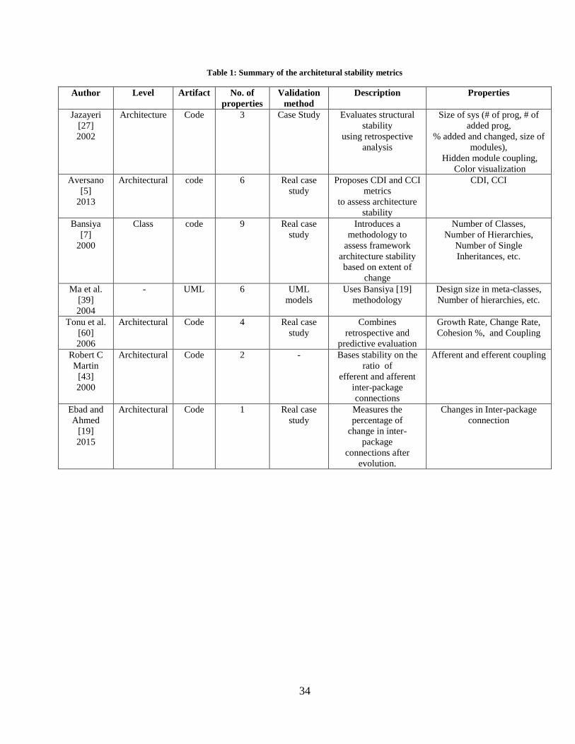
34
Table 1: Summary of the architetural stability metrics
Author Level Artifact No. of
properties
Validation
method
Description Properties
Jazayeri
[27]
2002
Architecture Code 3 Case Study Evaluates structural
stability
using retrospective
analysis
Size of sys (# of prog, # of
added prog,
% added and changed, size of
modules),
Hidden module coupling,
Color visualization
Aversano
[5]
2013
Architectural code 6 Real case
study
Proposes CDI and CCI
metrics
to assess architecture
stability
CDI, CCI
Bansiya
[7]
2000
Class code 9 Real case
study
Introduces a
methodology to
assess framework
architecture stability
based on extent of
change
Number of Classes,
Number of Hierarchies,
Number of Single
Inheritances, etc.
Ma et al.
[39]
2004
- UML 6 UML
models
Uses Bansiya [19]
methodology
Design size in meta-classes,
Number of hierarchies, etc.
Tonu et al.
[60]
2006
Architectural Code 4 Real case
study
Combines
retrospective and
predictive evaluation
Growth Rate, Change Rate,
Cohesion %, and Coupling
Robert C
Martin
[43]
2000
Architectural Code 2 - Bases stability on the
ratio of
efferent and afferent
inter-package
connections
Afferent and efferent coupling
Ebad and
Ahmed
[19]
2015
Architectural Code 1 Real case
study
Measures the
percentage of
change in inter-
package
connections after
evolution.
Changes in Inter-package
connection
35
3 CHAPTER 3
RESEARCH METHODOLOGY
3.1 Fitness function for Functionality-based software packaging using
sequence diagrams
The main idea in this work is to enable packaging decisions right from architectural design
level rather than the source code level, using the sequence diagrams. A sequence diagrams
realize a use case.
There are two popular and competing objectives in software design and organization. First
is the desire to have loosely (lowly) coupled system parts and second is the desire to have
highly cohesive system parts. In this context loose coupling implies that each use case
should consider the least number of packages. Loose coupling reflects that the packages
are self-contained, and offers a complete function with as little dependency on other
packages as possible. While high cohesion implies that the classes in each package are
related to each other and that they contribute the same use case.
Thus, this are the two main goals (objectives) considered in the development of the fitness
function for software packaging. We call them usecase coverage and class relevancy
respectively.
Therefore, the two objective can be combined formulate a single objective called
overallpackaging of a system. Going by the principle of Occam's razor mentioned earlier,
the two objectives can be linearly combined as follows:

36
Ebad and Ahmed [20] defined the overallPackaging metric as:
OverallPackaging(system) = Avg(PackagingQlty(Pi))
where: PackagingQlty(Pi)) is the packaging quality of a package Pi, and is calculated
as:
PackagingQlty(Pi) = Wu × degree of UC coverage by Pi
+ Wc × degree of class relevancy of Pi
where: Wu is the weight of the UC’s coverage in a package and Wc is the weight of the
class relevancy in a package, so that Wu, Wc ∈ [0, 1] and Wu + Wc = 1.More details about
the definition of the metric can be found at [20].
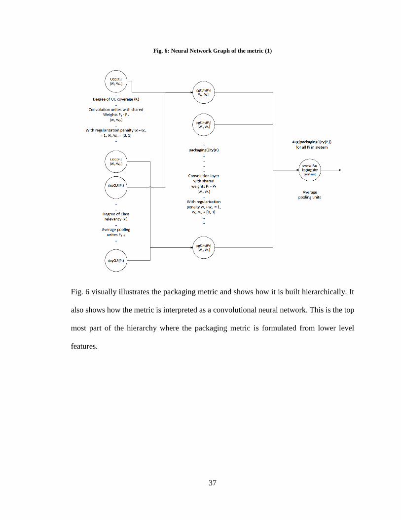
37
Fig. 6: Neural Network Graph of the metric (1)
Fig. 6 visually illustrates the packaging metric and shows how it is built hierarchically. It
also shows how the metric is interpreted as a convolutional neural network. This is the top
most part of the hierarchy where the packaging metric is formulated from lower level
features.

38
Fig. 7: Neural Network Graph of the metric (2)
Fig. 7 visually illustrates the packaging metric and shows how it is built hierarchically. It
also shows how the metric is interpreted as a convolutional neural network. This is the
second level after the top most part of the hierarchy where the packaging metric is
formulated from lower level features.
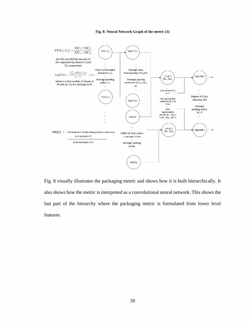
39
Fig. 8: Neural Network Graph of the metric (3)
Fig. 8 visually illustrates the packaging metric and shows how it is built hierarchically. It
also shows how the metric is interpreted as a convolutional neural network. This shows the
last part of the hierarchy where the packaging metric is formulated from lower level
features.

40
3.1.1 Degree of UC coverage
The Degree of UC coverage measures how well a package confines itself to just realization
of minimum number of UCs as possible.
Degree of UC coverage by a package P, can be seen as a composition of two lower level
factors: (1) the percentage of UC interaction performed within P, and (2) the provision of
methods for the UC’s SD from within P.
The interaction factor can be further divided into two types, direct and indirect. Direct
interaction implies method call involving a method calling another one directly as opposed
to through some other methods.
Given usecase UCj from set of UCs of the system and package Pi from set of packages in
the packaging configuration of the system. Let D be the number of method calls in the
intersection of direct method calls within UCj and Pi. Let T be the number of method calls
in the intersection of indirect method calls within UCj and Pi.
Further, let TD be the total number of direct method calls and TT the total number of
indirect (transitive) method calls of UCj.
Therefore, to compute the ratio of UCj method calls performed within package Pi, Ij(Pi) is
calculated as:
𝑰𝒋(𝑷𝒊) = 𝒘𝑫 ×𝑫+𝒘𝑻 ×𝑻
𝒘𝑫 ×𝑻𝑫+𝒘𝑻 ×𝑻𝑻[20]
Where wD and wT are weights for the direct and indirect method calls, respectively,
and since wD, wT ∈ [0, 1], wD + wT = 1.
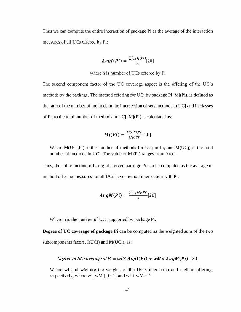
41
Thus we can compute the entire interaction of package Pi as the average of the interaction
measures of all UCs offered by Pi:
𝑨𝒗𝒈𝑰(𝑷𝒊) = ∑ 𝑰𝒋(𝑷𝒊)𝒏
𝒋=𝟏
𝒏[20]
where n is number of UCs offered by Pi
The second component factor of the UC coverage aspect is the offering of the UC’s
methods by the package. The method offering for UCj by package Pi, Mj(Pi), is defined as
the ratio of the number of methods in the intersection of sets methods in UCj and in classes
of Pi, to the total number of methods in UCj. Mj(Pi) is calculated as:
𝑴𝒋(𝑷𝒊) = 𝑴(𝑼𝑪𝒋,𝑷𝒊)
𝑴(𝑼𝑪𝒋)[20]
Where M(UCj,Pi) is the number of methods for UCj in Pi, and M(UCj) is the total
number of methods in UCj. The value of Mj(Pi) ranges from 0 to 1.
Thus, the entire method offering of a given package Pi can be computed as the average of
method offering measures for all UCs have method intersection with Pi:
𝑨𝒗𝒈𝑴(𝑷𝒊) = ∑ 𝑴𝒋(𝑷𝒊)𝒏
𝒋=𝟏
𝒏[20]
Where n is the number of UCs supported by package Pi.
Degree of UC coverage of package Pi can be computed as the weighted sum of the two
subcomponents facors, I(UCi) and M(UCi), as:
Degree of UC coverage of Pi = wI × 𝑨𝒗𝒈𝑰(𝑷𝒊) + wM × 𝑨𝒗𝒈𝑴(𝑷𝒊) [20]
Where wI and wM are the weights of the UC’s interaction and method offering,
respectively, where wI, wM [ [0, 1] and wI + wM = 1.

42
3.1.2 Degree of class relevancy
Class relevancy is formulated as a composition of two lower level factor: class functionality
(CF) and class utilization (Util).
consider two classes C1 and C2. Let UC1 and UC2 be two sets of UCs that uses C1 and
C2, respectively. If |UC1 ∪ UC2| and |UC1 ∩ UC2| the cardinality of the union and
intersection of both sets respectively, then, we can define class functionality between two
classes C1 and C2 as:
CF(C1,C2) = |𝑼𝑪𝟏 ∩ 𝑼𝑪𝟐|
|𝑼𝑪𝟏∪𝑼𝑪𝟐|[20].
Where a CF value of 0 indicates no common UCs shared by the two classes and a value
of 1 indicates that both classes support the exact same UCs.
Therefore for a given class Ci in package Pk, the average CF, AvgCF can be computed as:
𝑨𝒗𝒈𝑪𝑭(𝑪𝒊) = ∑ 𝑪𝑭(𝑪𝒊,𝑪𝒋)𝒏
𝒋=𝟏
𝒏−𝟏[20]
Where n is the number of classes in Pk and Cj, 1 ≤ j ≤ n, belongs to Pk.
The second factor that composes the degree of class relevancy is Util. This measures the
degree of utility of a class by computing the percentage of methods of the class that make
call(s) within the package. Given class Ci in package Pk, Ci utility can be computed as:
Util(Ci,Pk) = # 𝒐𝒇 𝒎𝒆𝒕𝒉𝒐𝒅𝒔 𝒊𝒏 𝑪𝒊 𝒊𝒏𝒕𝒆𝒓𝒂𝒄𝒕𝒊𝒏𝒈 𝒘𝒊𝒕𝒉 𝒎𝒆𝒕𝒉𝒐𝒅𝒔 𝒊𝒏 𝑷𝒌
# 𝒐𝒇 𝒎𝒆𝒕𝒉𝒐𝒅𝒔 𝒊𝒏 𝑪𝒊[20]
The relevancy of class Ci in package Pk can be calculated as the combination of its CF and
Util as:
𝑪𝑹(𝑪𝒊) = 𝒘𝑭 × 𝑨𝒗𝒈𝑪𝑭(𝑪𝒊) + 𝒘𝑼𝒕 × 𝑼𝒕𝒊𝒍(𝑪𝒊, 𝑷𝒌)[20]

43
Where wF and wUt are the weights of the class functionality and class utilization,
respectively.
Hence, degree of class relevancy of a package is computed as the average of the class
relevancy for all classes in that package. Degree of class relevancy of package Pk is
computed as:
Degree of Class relevancy of Pk = Avg(CR(Cj))[20]
Now by aggregation of the previous formulas, the overall packaging quality,
overallPackaging of the entire system is computed as average of all PackagingQlty each
packages in the system:
OverallPackaging(system) = Avg(PackagingQlty(Pi)) [20]
Hence, from this formulation, the OverallPackaging should be maximized to achieve a
higher quality packaging configuration.
Given a hypothetical sequence diagrams (SDs) shown in Fig. 10, Fig. 11 , and Fig. 12 with
a sample configuration shown in Fig. 9, the overallPackaging(system) can be calculated as
shown in Table 2. All weights being set to 0.5. More detail of how the calculations are
arrived at is given by Ebad and Ahmed [20].
Table 2: showing calculation of overall packaging of the system
P1 P2
PackagingQlty 0.5 (0.5) + 0.5 (0.72) = 0.61 0.5 (0.41) + 0.5 (.6) = 0.51
OverallPackaging (0.61 + 0.51)/2 = 0.56
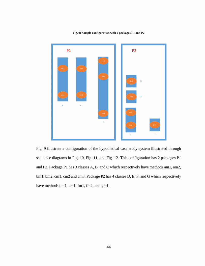
44
Fig. 9: Sample configuration with 2 packages P1 and P2
Fig. 9 illustrate a configuration of the hypothetical case study system illustrated through
sequence diagrams in Fig. 10, Fig. 11, and Fig. 12. This configuration has 2 packages P1
and P2. Package P1 has 3 classes A, B, and C which respectively have methods am1, am2,
bm1, bm2, cm1, cm2 and cm3. Package P2 has 4 classes D, E, F, and G which respectively
have methods dm1, em1, fm1, fm2, and gm1.

45
Fig. 10: UC1 being realized by SD
Fig. 10 illustrates the sequence diagram (SD) of the hypothetical system involving
sequence of communications between methods of 3 different classes (A, B, and C
respectively) of the hypothetical system.
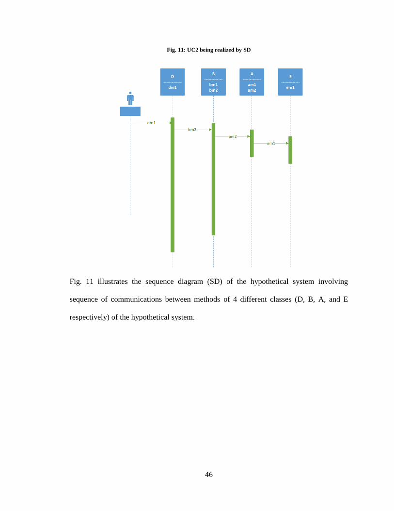
46
Fig. 11: UC2 being realized by SD
Fig. 11 illustrates the sequence diagram (SD) of the hypothetical system involving
sequence of communications between methods of 4 different classes (D, B, A, and E
respectively) of the hypothetical system.
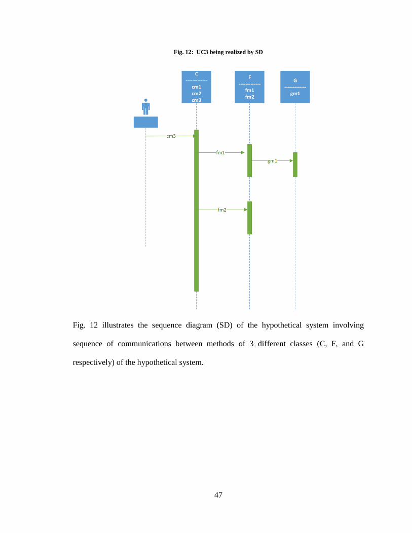
47
Fig. 12: UC3 being realized by SD
Fig. 12 illustrates the sequence diagram (SD) of the hypothetical system involving
sequence of communications between methods of 3 different classes (C, F, and G
respectively) of the hypothetical system.

48
3.2 Problem solving
3.2.1 Model extension
Outlined earlier were steps to be taken to identifying, analyzing, formulating and solving
an optimization (multi or single objective) problem. This will serve as a guide for research
pursuing this endeavor.
It is clearly showed ways in which an objective function can be formulated. I have shown
clearly the relationship between machine learning and optimization. Helping new and
novice researchers understand what they mean and how they relate.
I have provided a neural network interpretation of the original model successful model and
thereby showed a clear path for feature research in automation of quantification and
qualification of software artifacts. This has pave way for applying and investigating several
neural network techniques in for packaging software systems.
This way we can acquire simple metrics and formulate different architecture of neural
networks then train them by using a training and validation dataset.
Consequently, neural network technique can be applied to other software engineering by
acquiring simple software metrics from good knowledge of metrics formulation or simply
by use of metric tools one can be able to develop a model for automatic quantification or
qualification of software artifacts.
This study helps to further strengthen and demonstrate the justification and popularity of
neural networks as current state-of-the-art in modeling.

49
So the lesson is, we should spend effort formulating latent features that are complicated
(and even incomprehensible that we even run out of how to name them) instead acquire
direct features as many of the direct features and let the neural network learn the higher
level feature by itself.
Fig. 13: Convolution Neural Network model interpretation and extension
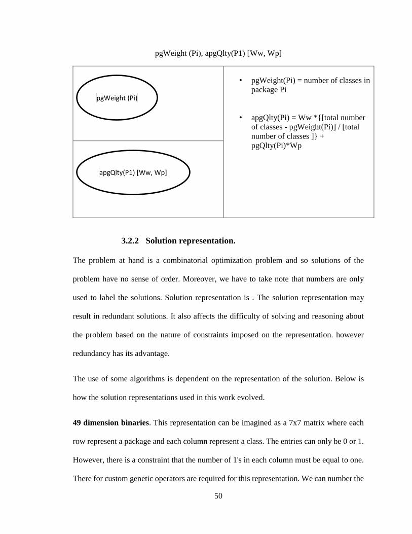
50
pgWeight (Pi), apgQlty(P1) [Ww, Wp]
• pgWeight(Pi) = number of classes in
package Pi
• apgQlty(Pi) = Ww *{[total number
of classes - pgWeight(Pi)] / [total
number of classes ]} +
pgQlty(Pi)*Wp
3.2.2 Solution representation.
The problem at hand is a combinatorial optimization problem and so solutions of the
problem have no sense of order. Moreover, we have to take note that numbers are only
used to label the solutions. Solution representation is . The solution representation may
result in redundant solutions. It also affects the difficulty of solving and reasoning about
the problem based on the nature of constraints imposed on the representation. however
redundancy has its advantage.
The use of some algorithms is dependent on the representation of the solution. Below is
how the solution representations used in this work evolved.
49 dimension binaries. This representation can be imagined as a 7x7 matrix where each
row represent a package and each column represent a class. The entries can only be 0 or 1.
However, there is a constraint that the number of 1's in each column must be equal to one.
There for custom genetic operators are required for this representation. We can number the
pgWeight (Pi)
apgQlty(P1) [Ww, Wp]

51
rows from top-down and columns left-right. This representation produces redundant
configurations. For example a solution with all 1's in row one is same as solution with all
ones in any other rows.
𝑐1 𝑐2 𝑐3 𝑐4 𝑐5 𝑐6 𝑐7𝑝1
𝑝2
𝑝3 1 1 1
𝑝4 1 1 1 1
𝑝5
𝑝6
𝑝7
7 dimensions of integers. This representation evolved from the previous one where each
dimension represents a class from the columns of the previous representation. The value
for the variable of a dimension comes from the row number of where 1 appears in that
column. So this can be used with algorithms that accept integer or real dimensions. For real
variable type, we have to round the value to a feasible integer. The constraints in this case
are min and max bounds that simpler than to enforce and assimilate than in the earlier
representation. It suffers from same redundancy as earlier.
𝑐1 𝑐2 𝑐3 𝑐4 𝑐5 𝑐6 𝑐73 3 3 4 4 4 4
1 integer rounded to boundaries. If we view the earlier representation as a 7 digits integer
then, we can represent our solution with a single 7 digits integer between 1111111 to

52
7777777. In this case, the constraint will be that integers in the range with any digit other
than from 1 to 7 constitute an invalid solution. For real variable type, we have to round the
value to a feasible integer to impose the constraint is not easy. One way to do it is that
whenever you have a 0 value digit it should be rounded to 1 and whenever you get 8 and 9
they should be rounded to 7. However, this has a problem as it is not consistent in ordering
of solutions. A question one may ask is how problem with 10 or more variable values can
be represented. This solution is to use a number base system to can take all the values of a
variable. It suffers from same redundancy as ealier first representation. Illustrate the
problem and explain why no need for the experiment.
1 integer array of all configurations. This solution representation evolved due to the
rounding problem of the earlier representation. So in this representation all valid
configurations are computed an stored in and array. It suffers from same redundancy as
earlier first representation. This may not be feasible if we have real dimension unless if
discretized or if the dimension of solution is very high it may also be infeasible to compute.
1 integer array of all configurations with elimination of repeated configurations. The
computation required to do this is not feasible in real application scenario because the
complexity is high. Give the algorithm to do it and the complexity analysis here. However
this representation will still be utilized for this case study scenario since the number of it
is relatively small. Using this helps make some analysis faster. This will be demonstrated
later on when analysing the penalty function or new objective formulation. Moreover since
the same solution is repeated many times the algorithm may be lucky to fine one out of
many.

53
Number of packages and constrained 7 dimensions based on number of packages.
This imposes a very harsh and difficult to maintain nonlinear constraint. Since this imposes
a nonlinear constraint, readymade genetic operators in the toolbox cannot be used to
achieve valid solution after each iteration. The variable number of packages make it
difficult to implement the crossover operators.
3.2.3 Architectural stability
Attempt was made to validate the metric using architectural stability metric. This validation
concept stems from an intuition that a well packaged software should be more stable and
be averse to too many changes. A metric by Ebad and Ahmed [19] called Architectural
Stability Metric (ASM) was considered for this task. ASM is metric purely based on inter-
package connections. Afterwards, extension was made to ASM called Extended
Architectural Stability Metric (ExASM) that considers both changes intra-package and
inter-package connections. Another metric CEAM (Coupling Efferent-Afferent Metric),
based on package instability metric proposed by Robert C Martin in his book [43], was
also used in this endeavor.
Formulation of both ASM and ExASM is outlined below:
• If R1 and R2 are two releases having two packages P1 and P2.
• Let:
– 𝐴𝑖𝑛𝑡𝑒𝑟 and 𝐴𝑖𝑛𝑡𝑟𝑎 be the set of added inter-PCs and Intra-PCs in R2,
– 𝐷𝑖𝑛𝑡𝑒𝑟 and 𝐷𝑖𝑛𝑡𝑟𝑎 be the set of deleted inter-PCs and intra-PCs from R1
– 𝑂𝑖𝑛𝑡𝑒𝑟 and 𝑂𝑖𝑛𝑡𝑟𝑎be the set of original inter-PCs and intra-PCs that exist in
R1
– ASMinter be inter-package ASM

54
– ASMintra be intra-package ASM
• ExASM(R1,R2) = w* ASMinter (R1,R2) + (1-w)* ASMintra (R1,R2)
• Where:
– w is user specified weight that balances between inter-PC and intra-PC
– ASMinter = |𝑂𝑖𝑛𝑡𝑒𝑟|−|𝐷𝑖𝑛𝑡𝑒𝑟|
|𝑂𝑖𝑛𝑡𝑒𝑟|+|𝐴𝑖𝑛𝑡𝑒𝑟|
– ASMintra = |𝑂𝑖𝑛𝑡𝑟𝑎|−|𝐷𝑖𝑛𝑡𝑟𝑎|
|𝑂𝑖𝑛𝑡𝑟𝑎|+|𝐴𝑖𝑛𝑡𝑟𝑎|
• ASM as formulated by Ebad and Ahmed is simply ASMinter as defined above.
• The proposed ExASM metric is theoretically validated and satisfies the seven
listed mathematical properties as follows.
– Non-negativity: It can be seen very easily that the metric as stated satisfies
this property.
– Normalization: The metric values clearly ranges between 0 and 1. The
metric will give 0 if no changes occur and will give 1 if there’s complete
change. That is the metric should have a clearly defined upper and lower
bounds
– Null value: This properties should hold in the case where there exist no
inter-PC and intra-PC between the two versions at all. This property is
satisfied with ExASM metric when both sets Ointer and Ointra are empty,
Implying, no PCs in Ri (the base release) in the first place.
– Maximum value: This property is also clearly satisfied and correspond to
the upper bound of normalization property
– Transitivity: This property ensures consistency of the metric evaluation. In
case where this are 3 different stability measures, then, if the 1st meausure
is better than the 2nd and the 2nd is better than the 3rd, then the 1st should
be better than the 3rd.
Formulation of Coupling Efferent-Afferent Metric (CEAM) is given as follows:
• Afferent couplings (Ca): this measures the dependency of a package in inwards by
counting the number of classes that outside of the package that depend on the
classes within the package.
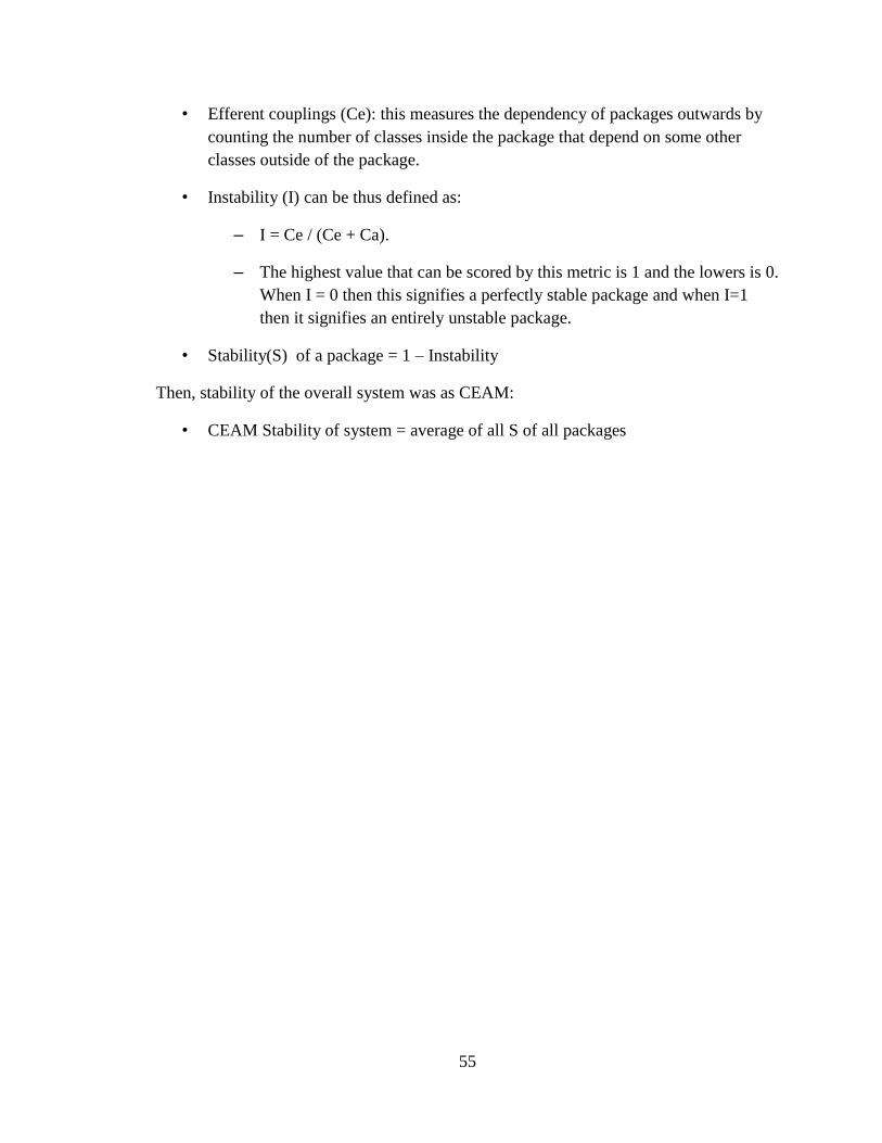
55
• Efferent couplings (Ce): this measures the dependency of packages outwards by
counting the number of classes inside the package that depend on some other
classes outside of the package.
• Instability (I) can be thus defined as:
– I = Ce / (Ce + Ca).
– The highest value that can be scored by this metric is 1 and the lowers is 0.
When I = 0 then this signifies a perfectly stable package and when I=1
then it signifies an entirely unstable package.
• Stability(S) of a package = 1 – Instability
Then, stability of the overall system was as CEAM:
• CEAM Stability of system = average of all S of all packages
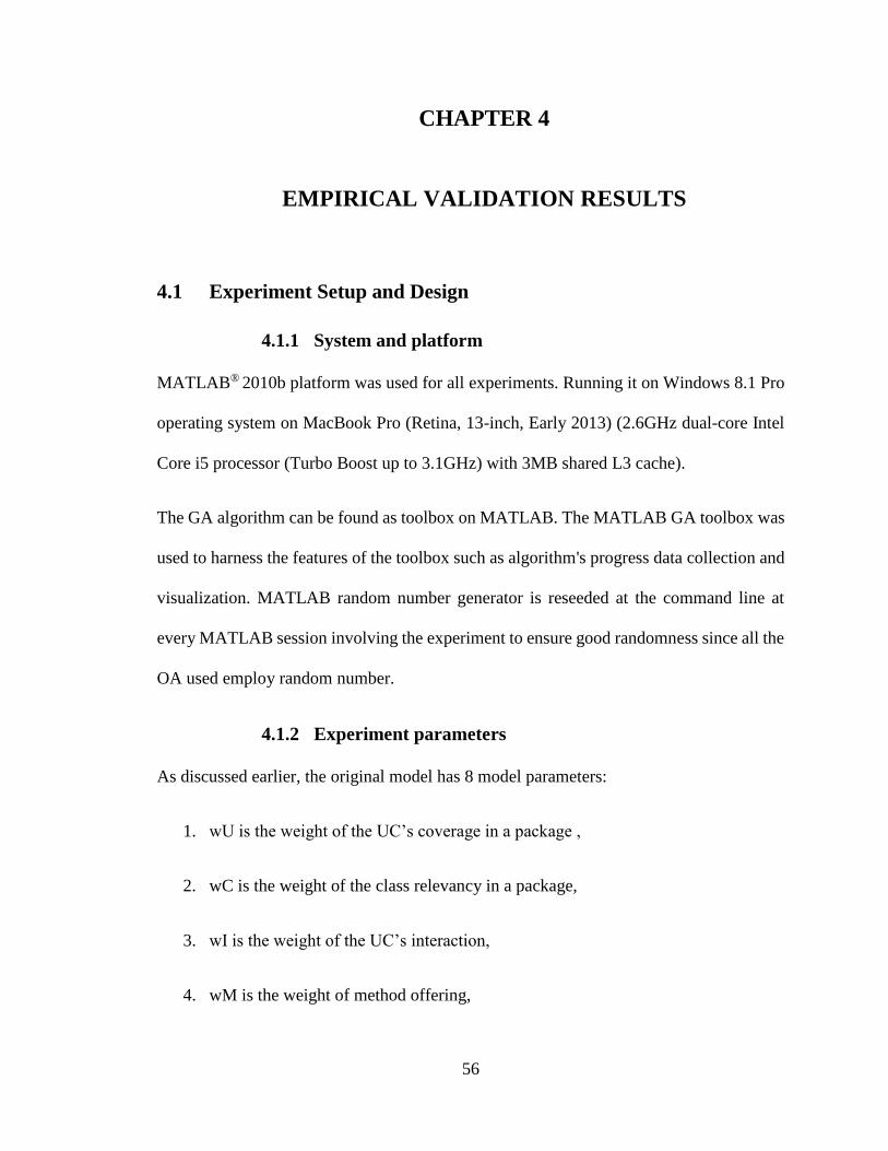
56
4 CHAPTER 4
EMPIRICAL VALIDATION RESULTS
4.1 Experiment Setup and Design
4.1.1 System and platform
MATLAB® 2010b platform was used for all experiments. Running it on Windows 8.1 Pro
operating system on MacBook Pro (Retina, 13-inch, Early 2013) (2.6GHz dual-core Intel
Core i5 processor (Turbo Boost up to 3.1GHz) with 3MB shared L3 cache).
The GA algorithm can be found as toolbox on MATLAB. The MATLAB GA toolbox was
used to harness the features of the toolbox such as algorithm's progress data collection and
visualization. MATLAB random number generator is reseeded at the command line at
every MATLAB session involving the experiment to ensure good randomness since all the
OA used employ random number.
4.1.2 Experiment parameters
As discussed earlier, the original model has 8 model parameters:
1. wU is the weight of the UC’s coverage in a package ,
2. wC is the weight of the class relevancy in a package,
3. wI is the weight of the UC’s interaction,
4. wM is the weight of method offering,

57
5. wD is the weight of direct interactions,
6. wT is the weight of indirect interactions,
7. wF is the weight of class functionality, and
8. wUt is the weight of class utilization.
4.1.3 Experiment design
Each instance of experiment was run 5 times (replications) so that the average output is
calculated as the result of that instance. Since grid search technique was used, numerical
value factors have to be discretized as all possible values cannot be tried. Even after
discretization, a full factorial design with replication will be too large. Therefore, a
fractional factorial design of n2m has to be used. However fractional factorial design is not
used to scale down the number of factors but to manually monitor how the changes in
parameter values affect result so we can have an idea about where a good set of values of
the parameters are.
4.2 Solution representation experiments
This was done as a preliminary experiments to decide what solution representation are
suitable. A single algorithm is enough to determine what solution representation is suitable.
GA was used for this task. The preliminary experiment is important to rapidly scale down
the number of experiments (run of algorithms).
As part of the preliminary experiment, analysis of the brute force algorithm is given. We
need to know attribute of the brute force algorithm so that we can compare and appreciate
the effort of the optimization algorithms. Number of function evaluation for the brute force

58
is at least number of configurations in 7 integer solution representation because all points
have to be evaluated at least once. It took 49815.628 seconds (approximately 14 hours) to
run the algorithm. When running the brute force algorithm, the score of each configuration
was saved to a permanent memory to be reused later so that it doesn't have to be calculated
at every function evaluation and thereby saving experiment time. Below is the plot of the
overallpackagingQlty against solutions.
The original model with model parameters set to (wU = 0.5; wC = 0.5; wI = 0.25; wM =
0.75; wD = 2/3; wT = 1/3; wF = 0.85; wUt = 0.15) was used in this experiment. These
parameter values are those recommended by Ebad an Ahmed [20] for getting intuitive
packageing. We used these setting because we do not want the optima to be at the boundary
as it will be if model is used as it is and parameter values are all set to 0.5 except for wD =
2/3 and wT = 1/3. Having optima points at the boundary does not help assess effectively
the performance of an OA.
GA with integer constraint was the only OA used in this case. The algorithm GA toolbox
uses for integer constraint optimization is based on the work of kusum et al. [13] In this
case, GA does not allow selection or specification of creation, crossover and mutation
functions. So the only 2 options necessary to tune are number of elites and crossover
fraction.
To illustrate the performance of each representation format, 2 media are used:
1. Table of average of best scores for the 5 runs of each instance combination of the
parameters.
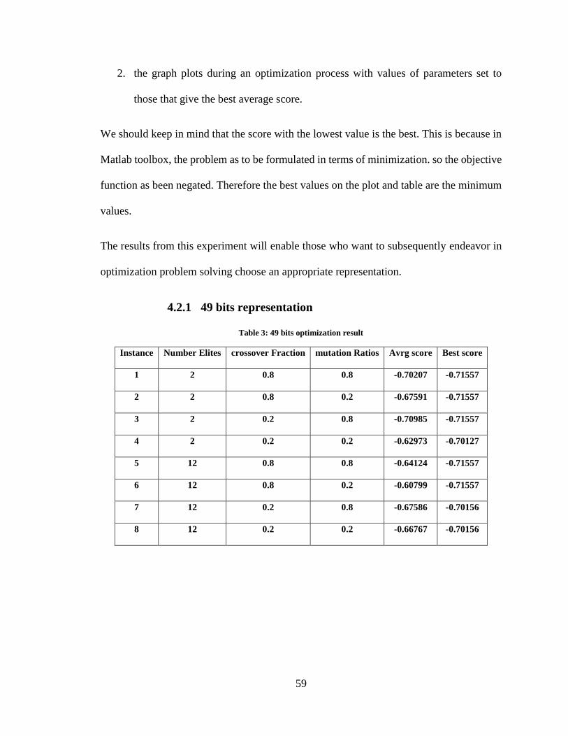
59
2. the graph plots during an optimization process with values of parameters set to
those that give the best average score.
We should keep in mind that the score with the lowest value is the best. This is because in
Matlab toolbox, the problem as to be formulated in terms of minimization. so the objective
function as been negated. Therefore the best values on the plot and table are the minimum
values.
The results from this experiment will enable those who want to subsequently endeavor in
optimization problem solving choose an appropriate representation.
4.2.1 49 bits representation
Table 3: 49 bits optimization result
Instance Number Elites crossover Fraction mutation Ratios Avrg score Best score
1 2 0.8 0.8 -0.70207 -0.71557
2 2 0.8 0.2 -0.67591 -0.71557
3 2 0.2 0.8 -0.70985 -0.71557
4 2 0.2 0.2 -0.62973 -0.70127
5 12 0.8 0.8 -0.64124 -0.71557
6 12 0.8 0.2 -0.60799 -0.71557
7 12 0.2 0.8 -0.67586 -0.70156
8 12 0.2 0.2 -0.66767 -0.70156
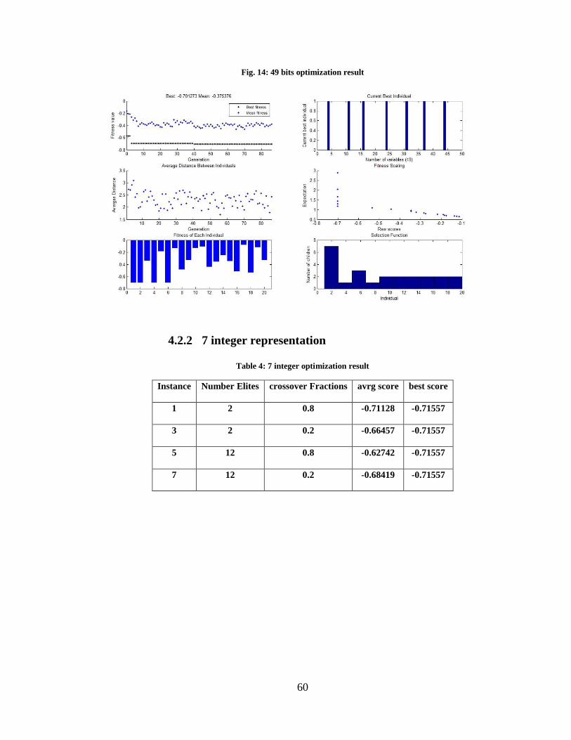
60
Fig. 14: 49 bits optimization result
4.2.2 7 integer representation
Table 4: 7 integer optimization result
Instance Number Elites crossover Fractions avrg score best score
1 2 0.8 -0.71128 -0.71557
3 2 0.2 -0.66457 -0.71557
5 12 0.8 -0.62742 -0.71557
7 12 0.2 -0.68419 -0.71557

61
Fig. 15: 7 integer optimization result
4.2.3 1 integer rounded
Table 5: 1 integer optimization result
Instance Number Elites crossover Fractiions Avrg score Best score
1 2 0.8 -0.63527 -0.71557
2 2 0.2 -0.69801 -0.71557
3 12 0.8 -0.62092 -0.70127
4 12 0.2 -0.64969 -0.71557
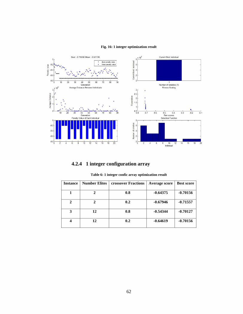
62
Fig. 16: 1 integer optimization result
4.2.4 1 integer configuration array
Table 6: 1 integer confic array optimization result
Instance Number Elites crossover Fractions Average score Best score
1 2 0.8 -0.64375 -0.70156
2 2 0.2 -0.67946 -0.71557
3 12 0.8 -0.54344 -0.70127
4 12 0.2 -0.64619 -0.70156
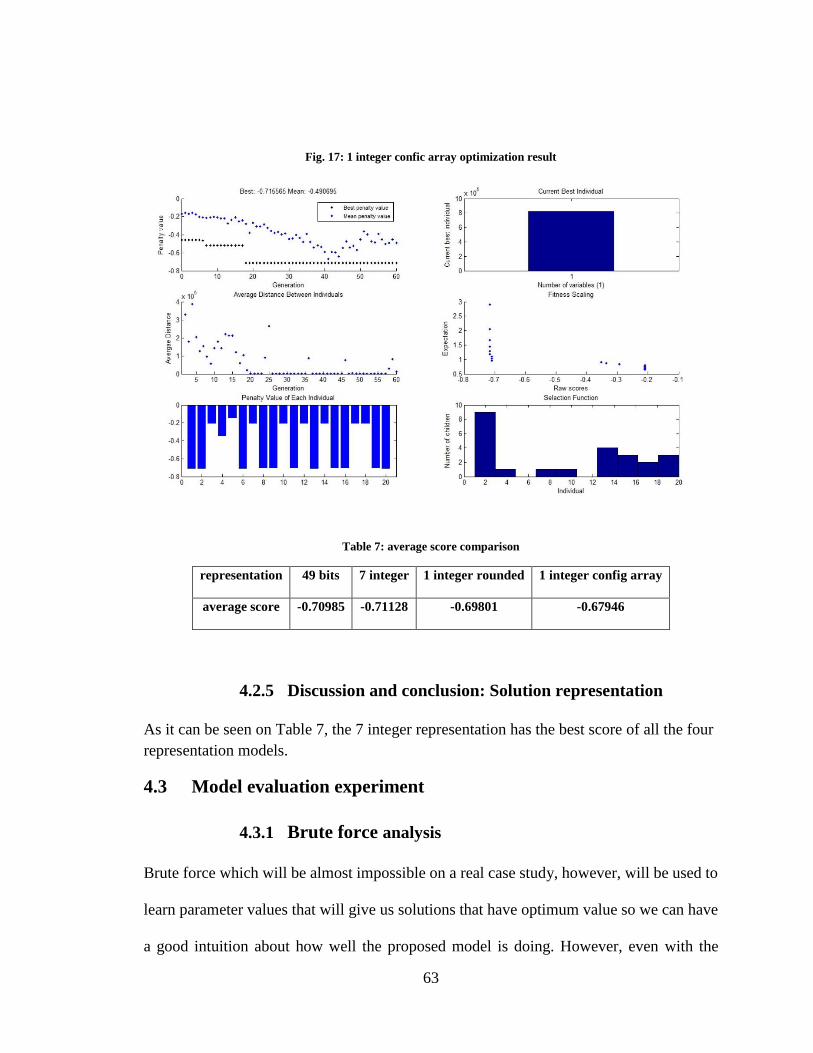
63
Fig. 17: 1 integer confic array optimization result
Table 7: average score comparison
representation 49 bits 7 integer 1 integer rounded 1 integer config array
average score -0.70985 -0.71128 -0.69801 -0.67946
4.2.5 Discussion and conclusion: Solution representation
As it can be seen on Table 7, the 7 integer representation has the best score of all the four
representation models.
4.3 Model evaluation experiment
4.3.1 Brute force analysis
Brute force which will be almost impossible on a real case study, however, will be used to
learn parameter values that will give us solutions that have optimum value so we can have
a good intuition about how well the proposed model is doing. However, even with the

64
miniature model (the hypothetical case study), the brute force will still take too much time.
In this case, the solution representation with 1 integer with elimination of repeated
configurations, becomes useful because it reduces the number of configurations to unique
packages and thereby reducing brute force run time significantly.
• All configurations Brute force analysis
• Unique configurations Brute force analysis
• fitness Brute force analysis
All configurations Brute force analysis
• number of all configurations (noclassesnoclasses) (for 7 classes 823543)
• algorithm complexity to get all configurations Omega(𝑛𝑛)
• time it takes to make all configurations
• for 7 classes 1.1289 secs
• For 50 classes 3.1825e+77
Unique configurations Brute force analysis
– number of unique configurations
• no way estimated by Gaussian
• for 7 classes 877 by brute force
– time it takes to make unique configurations
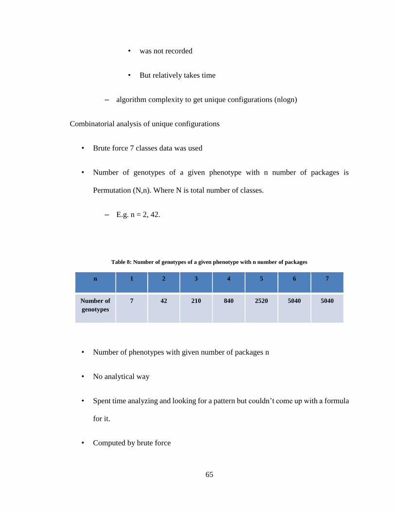
65
• was not recorded
• But relatively takes time
– algorithm complexity to get unique configurations (nlogn)
Combinatorial analysis of unique configurations
• Brute force 7 classes data was used
• Number of genotypes of a given phenotype with n number of packages is
Permutation (N,n). Where N is total number of classes.
– E.g. n = 2, 42.
Table 8: Number of genotypes of a given phenotype with n number of packages
n 1 2 3 4 5 6 7
Number of
genotypes
7 42 210 840 2520 5040 5040
• Number of phenotypes with given number of packages n
• No analytical way
• Spent time analyzing and looking for a pattern but couldn’t come up with a formula
for it.
• Computed by brute force
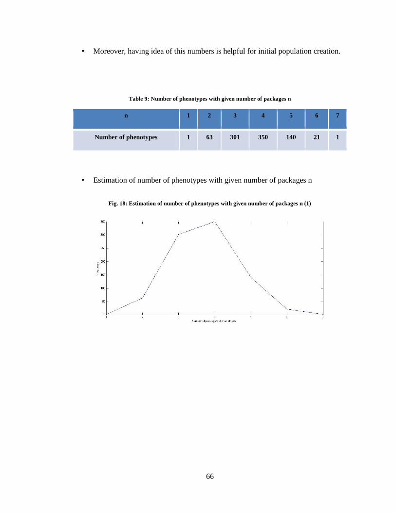
66
• Moreover, having idea of this numbers is helpful for initial population creation.
Table 9: Number of phenotypes with given number of packages n
n 1 2 3 4 5 6 7
Number of phenotypes 1 63 301 350 140 21 1
• Estimation of number of phenotypes with given number of packages n
Fig. 18: Estimation of number of phenotypes with given number of packages n (1)
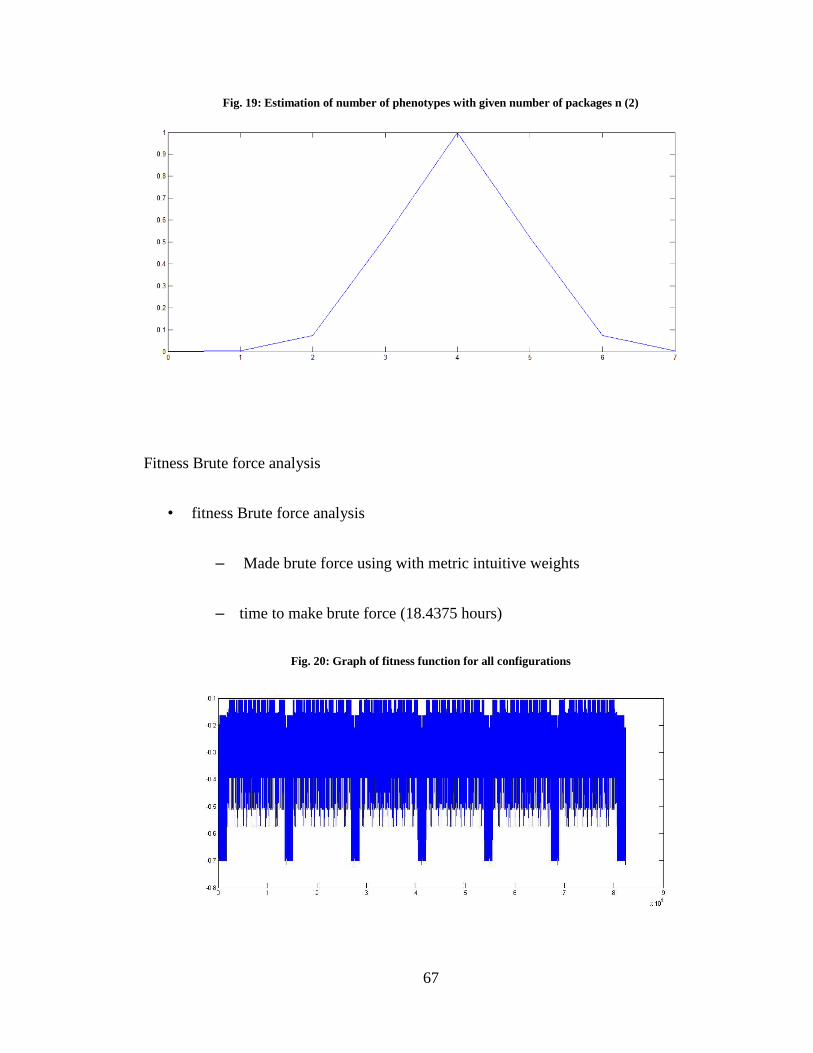
67
Fig. 19: Estimation of number of phenotypes with given number of packages n (2)
Fitness Brute force analysis
• fitness Brute force analysis
– Made brute force using with metric intuitive weights
– time to make brute force (18.4375 hours)
Fig. 20: Graph of fitness function for all configurations
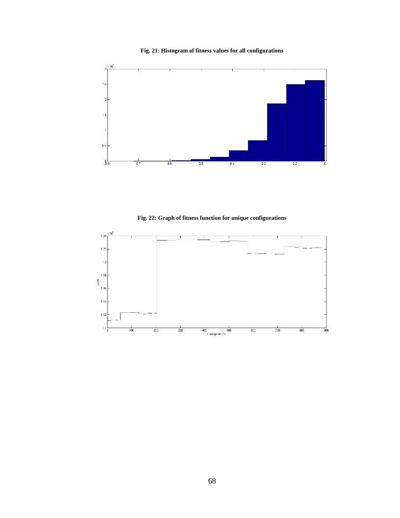
68
Fig. 21: Histogram of fitness values for all configurations
Fig. 22: Graph of fitness function for unique configurations

69
Fig. 23: Histogram of fitness values for unique configurations
4.3.2 Convolution Neural Network model evaluation
Expert's suggestion
In the work of [20] the configurations that were reported to march with experts suggestion
are given in Table 10.
Looking at Table 10, there are two factors we have learnt about in all the configurations.
number of packages
associated classes
All the four configurations have 2 or 3 number of packages. So our suggested optima
should have same or something very similar.
Looking at the table we also learned that certain classes are almost always packaged
together. Classes A and B, D and E, and F and G. where it seems it doesn't really matter
where C is.
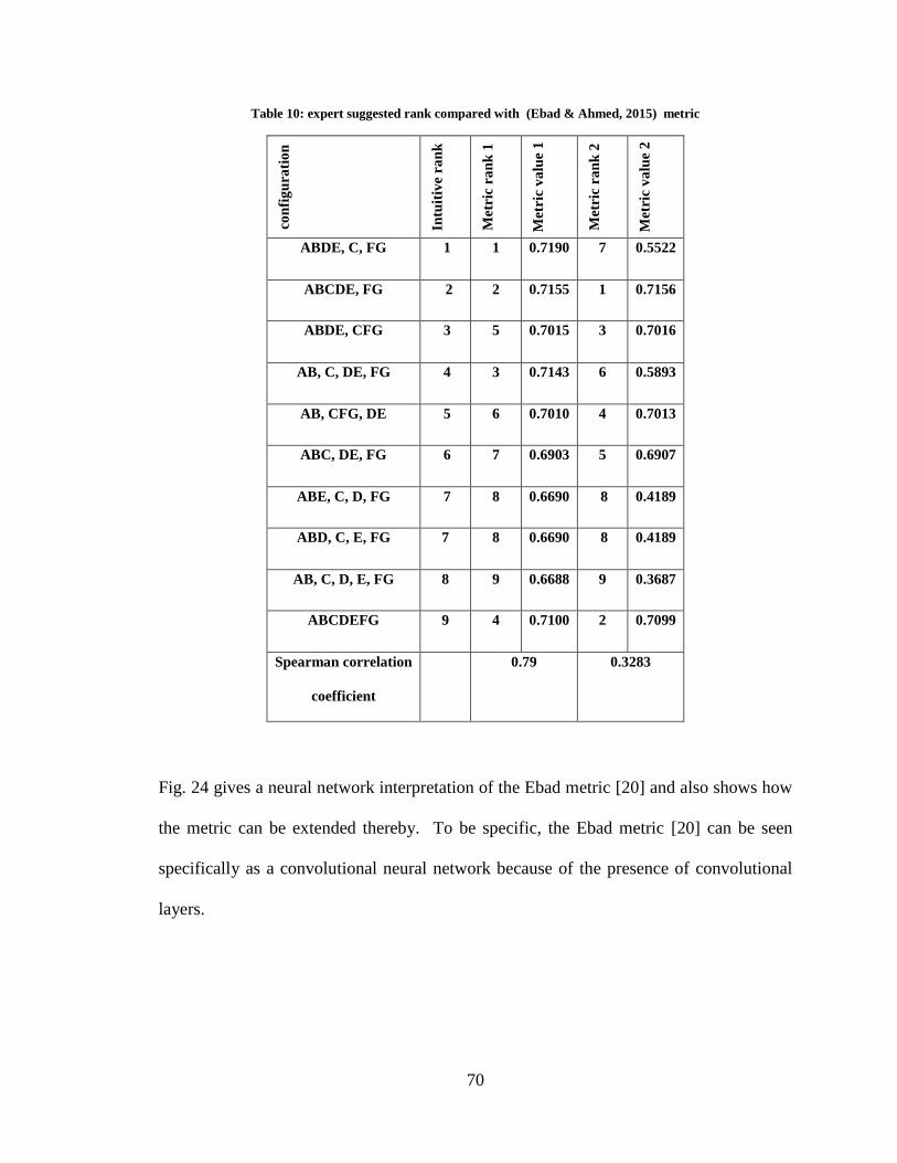
70
Table 10: expert suggested rank compared with (Ebad & Ahmed, 2015) metric
con
fig
ura
tio
n
Intu
itiv
e ra
nk
Met
ric
ran
k 1
Met
ric
va
lue
1
Met
ric
ran
k 2
Met
ric
va
lue
2
ABDE, C, FG 1 1 0.7190 7 0.5522
ABCDE, FG 2 2 0.7155 1 0.7156
ABDE, CFG 3 5 0.7015 3 0.7016
AB, C, DE, FG 4 3 0.7143 6 0.5893
AB, CFG, DE 5 6 0.7010 4 0.7013
ABC, DE, FG 6 7 0.6903 5 0.6907
ABE, C, D, FG 7 8 0.6690 8 0.4189
ABD, C, E, FG 7 8 0.6690 8 0.4189
AB, C, D, E, FG 8 9 0.6688 9 0.3687
ABCDEFG 9 4 0.7100 2 0.7099
Spearman correlation
coefficient
0.79 0.3283
Fig. 24 gives a neural network interpretation of the Ebad metric [20] and also shows how
the metric can be extended thereby. To be specific, the Ebad metric [20] can be seen
specifically as a convolutional neural network because of the presence of convolutional
layers.
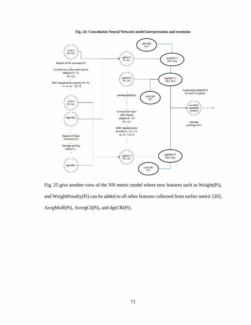
71
Fig. 24: Convolution Neural Network model interpretation and extension
Fig. 25 give another view of the NN metric model where new features such as Weight(Pi),
and WeightPenalty(Pi) can be added to all other features collected from earlier metric [20],
AvrgMoff(Pi), AvergCI(Pi), and dgrCR(Pi).
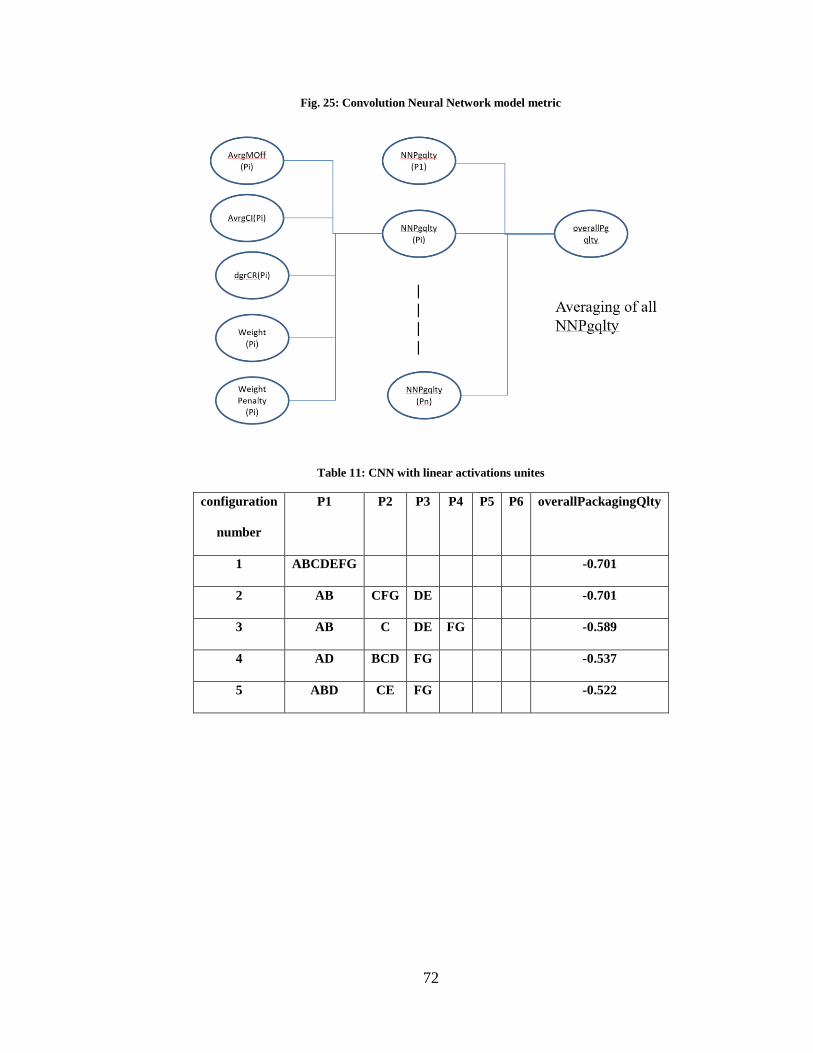
72
Fig. 25: Convolution Neural Network model metric
Table 11: CNN with linear activations unites
configuration
number
P1 P2 P3 P4 P5 P6 overallPackagingQlty
1 ABCDEFG -0.701
2 AB CFG DE -0.701
3 AB C DE FG -0.589
4 AD BCD FG -0.537
5 ABD CE FG -0.522

73
Table 12: CNN with logistic activation unites
configuration number P1 P2 P3 P4 P5 P6 overallPackagingQlty
1 AB CFG DE -0.754
2 ABCDEFG -0.597
3 ABE CFG D -0.582
4 A BDE CFG -0.446
5 AD BE CFG -0.383
Discussion and conclusion: CNN model interpretation and extension
Table 11 shows result of using neural network implemented on Matlab NN toolbox to
implement the Ebad metric. The network was implemented with all activation unites being
linear activation function. The table shows the top 5 configurations from that
implementation. For the matching configurations, on both Table 10 and Table 11 the
overallPackagingQlty score give the same value. As it can be seen for the case of
configuration ABCDEFG, AB, CFG, DE and AB, C, DE, FG.
Table 12 shows result of using neural network implemented on Matlab NN toolbox. The
network was implemented with all activation unites being logistic activation function.
Logistic activation function is what is widely used in conventional neural network
implementation. The table shows the top 5 configurations from that implementation. This
was experiment was conducted to illustrate that the metric can be interpreted as neural
networked and extended thereby.
Hypothesis 1: The metric used by Ebad and Ahmed [20] can be reinterpreted and extended
to make a better software packaging metric. This hypothesis has been partially fulfilled by
an interpretation of the metric as convolutional neural network and extension of the metric
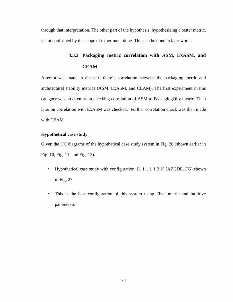
74
through that interpretation. The other part of the hypothesis, hypothesizing a better metric,
is not confirmed by the scope of experiment done. This can be done in later works.
4.3.3 Packaging metric correlation with ASM, ExASM, and
CEAM
Attempt was made to check if there’s correlation between the packaging metric and
architectural stability metrics (ASM, ExASM, and CEAM). The first experiment in this
category was an attempt on checking correlation of ASM to PackagingQlty metric. Then
later on correlation with ExASM was checked. Further correlation check was then made
with CEAM.
Hypothetical case study
Given the UC diagrams of the hypothetical case study system in Fig. 26 (shown earlier in
Fig. 10, Fig. 11, and Fig. 12).
• Hypothetical case study with configuration: [1 1 1 1 1 2 2] [ABCDE, FG] shown
in Fig. 27.
• This is the best configuration of this system using Ebad metric and intuitive
parameters
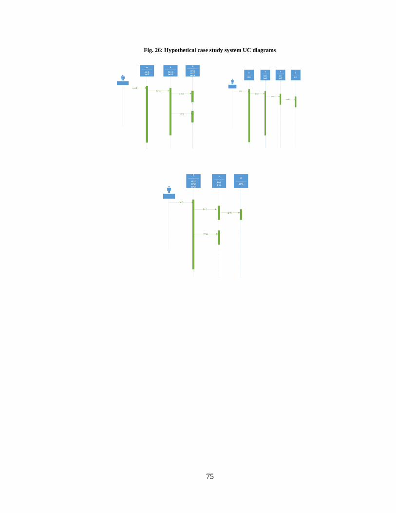
75
Fig. 26: Hypothetical case study system UC diagrams
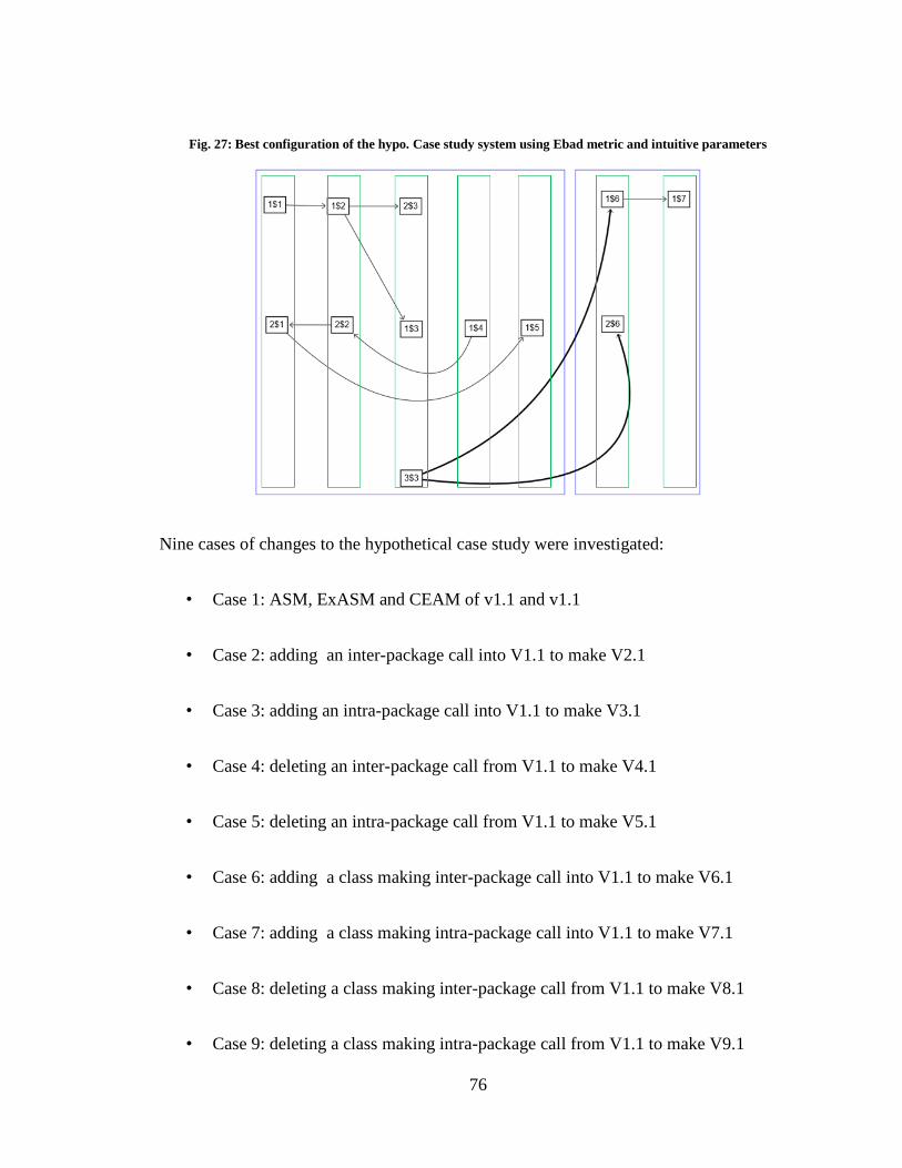
76
Fig. 27: Best configuration of the hypo. Case study system using Ebad metric and intuitive parameters
Nine cases of changes to the hypothetical case study were investigated:
• Case 1: ASM, ExASM and CEAM of v1.1 and v1.1
• Case 2: adding an inter-package call into V1.1 to make V2.1
• Case 3: adding an intra-package call into V1.1 to make V3.1
• Case 4: deleting an inter-package call from V1.1 to make V4.1
• Case 5: deleting an intra-package call from V1.1 to make V5.1
• Case 6: adding a class making inter-package call into V1.1 to make V6.1
• Case 7: adding a class making intra-package call into V1.1 to make V7.1
• Case 8: deleting a class making inter-package call from V1.1 to make V8.1
• Case 9: deleting a class making intra-package call from V1.1 to make V9.1

77
The detailed figures demonstrating all these cases can be found in
Appendix 1 from Table 33 to Table 75.
The nine cases were also used to tune the weight parameter called Weight of ExASM.
Eleven values of Weight ranging from 0 to 1 with 0.1 intervals. Change in packaging
quality (ChangeInPgQlty) was plotted against ExASM for the eleven values. The highest
absolute correlation coefficient (corr. Coef.) recorded is 0.7053 when value of Weight is
set to 0.4. The correlation figure for Weight = 0.4 is shown in Fig. 32. The figures showing
results for other values of Weight can be seen in Fig. 28, Fig. 29, Fig. 30, Fig. 31, Fig. 33,
Fig. 34, Fig. 35, Fig. 36, Fig. 37, and Fig. 38.
The corr. coef. R, is quiet close for almost all the different values of Weight. This can be
seen on table Table 13. For Weight value 0 corr. coef. is 0.43118 as shown in Fig. 28. For
Weight value 0.1 corr. coef. is 0.59118 as shown in Fig. 29. For Weight value 0.2 corr.
coef. is 0.67436 as shown in Fig. 30. For Weight value 0.3 corr. coef. is 0.70276 as shown
in Fig. 31. For Weight value 0.4 corr. coef. is 0.70530 as shown in Fig. 32. For Weight
value 0.5 corr. coef. is 0.69801 as shown in Fig. 33. For Weight value 0.6 corr. coef. is
0.68777 as shown in Fig. 34. For Weight value 0.7 corr. coef. is 0.67726 as shown in Fig.
35. For Weight value 0.8 corr. coef. is 0.66743 as shown in Fig. 36. For Weight value 0.9
corr. coef. is 0.65857 as shown in Fig. 37. For Weight value 1 corr. coef. is 0.65068 as
shown in Fig. 38.
To illustrate this point the average of all the corr. coef. is calculated as 0.6495 and the
standard deviation is 0.005693. As it can be seen the standard deviation is quiet small
indicating no much variation between the values of the corr. coef. This led us to conclude
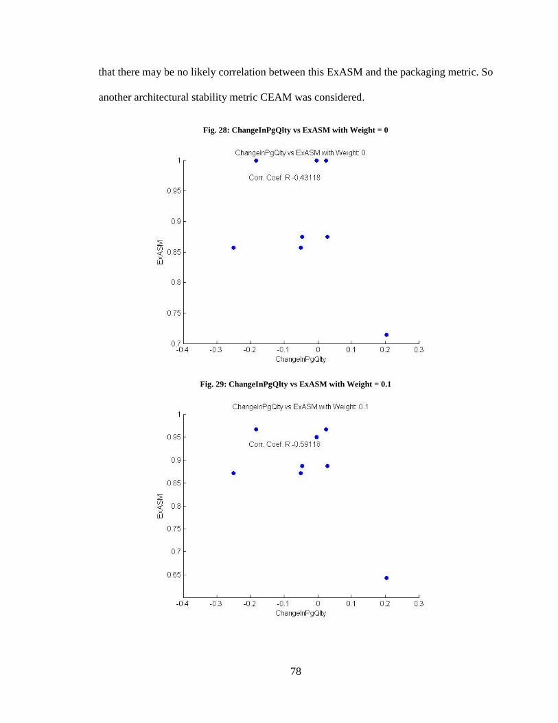
78
that there may be no likely correlation between this ExASM and the packaging metric. So
another architectural stability metric CEAM was considered.
Fig. 28: ChangeInPgQlty vs ExASM with Weight = 0
Fig. 29: ChangeInPgQlty vs ExASM with Weight = 0.1
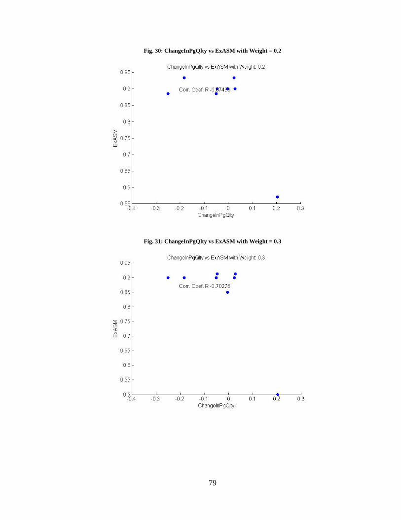
79
Fig. 30: ChangeInPgQlty vs ExASM with Weight = 0.2
Fig. 31: ChangeInPgQlty vs ExASM with Weight = 0.3

80
Fig. 32: ChangeInPgQlty vs ExASM with Weight = 0.4
Fig. 33: ChangeInPgQlty vs ExASM with Weight = 0.5
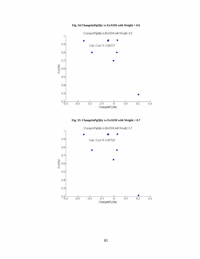
81
Fig. 34:ChangeInPgQlty vs ExASM with Weight = 0.6
Fig. 35: ChangeInPgQlty vs ExASM with Weight = 0.7
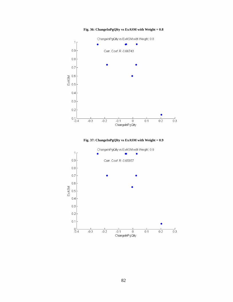
82
Fig. 36: ChangeInPgQlty vs ExASM with Weight = 0.8
Fig. 37: ChangeInPgQlty vs ExASM with Weight = 0.9
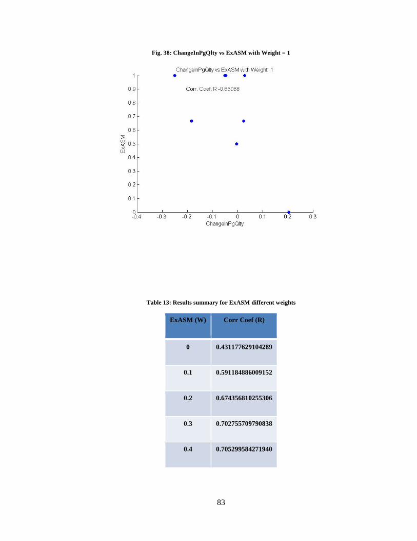
83
Fig. 38: ChangeInPgQlty vs ExASM with Weight = 1
Table 13: Results summary for ExASM different weights
ExASM (W) Corr Coef (R)
0 0.431177629104289
0.1 0.591184886009152
0.2 0.674356810255306
0.3 0.702755709790838
0.4 0.705299584271940
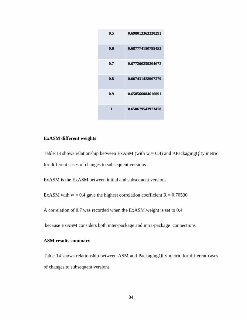
84
0.5 0.698013363330291
0.6 0.687774150795452
0.7 0.677260259204672
0.8 0.667431428007379
0.9 0.658566084616091
1 0.650679543973478
ExASM different weights
Table 13 shows relationship between ExASM (with w = 0.4) and ΔPackagingQlty metric
for different cases of changes to subsequent versions
ExASM is the ExASM between initial and subsequent versions
ExASM with w = 0.4 gave the highest correlation coefficient R = 0.70530
A correlation of 0.7 was recorded when the ExASM weight is set to 0.4
because ExASM considers both inter-package and intra-package connections
ASM results summary
Table 14 shows relationship between ASM and PackagingQlty metric for different cases
of changes to subsequent versions
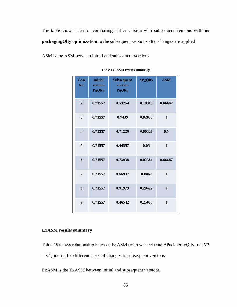
85
The table shows cases of comparing earlier version with subsequent versions with no
packagingQlty optimization to the subsequent versions after changes are applied
ASM is the ASM between initial and subsequent versions
Table 14: ASM results summary
Case
No.
Initial
version
PgQlty
Subsequent
version
PgQlty
ΔPgQlty ASM
2 0.71557 0.53254 0.18303 0.66667
3 0.71557 0.7439 0.02833 1
4 0.71557 0.71229 0.00328 0.5
5 0.71557 0.66557 0.05 1
6 0.71557 0.73938 0.02381 0.66667
7 0.71557 0.66937 0.0462 1
8 0.71557 0.91979 0.20422 0
9 0.71557 0.46542 0.25015 1
ExASM results summary
Table 15 shows relationship between ExASM (with w = 0.4) and ΔPackagingQlty (i.e. V2
– V1) metric for different cases of changes to subsequent versions
ExASM is the ExASM between initial and subsequent versions
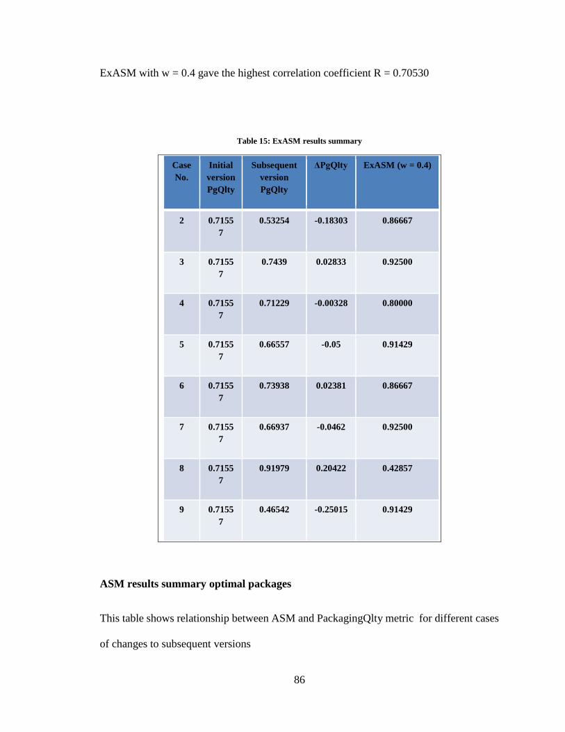
86
ExASM with w = 0.4 gave the highest correlation coefficient R = 0.70530
Table 15: ExASM results summary
Case
No.
Initial
version
PgQlty
Subsequent
version
PgQlty
ΔPgQlty ExASM (w = 0.4)
2 0.7155
7
0.53254 -0.18303 0.86667
3 0.7155
7
0.7439 0.02833 0.92500
4 0.7155
7
0.71229 -0.00328 0.80000
5 0.7155
7
0.66557 -0.05 0.91429
6 0.7155
7
0.73938 0.02381 0.86667
7 0.7155
7
0.66937 -0.0462 0.92500
8 0.7155
7
0.91979 0.20422 0.42857
9 0.7155
7
0.46542 -0.25015 0.91429
ASM results summary optimal packages
This table shows relationship between ASM and PackagingQlty metric for different cases
of changes to subsequent versions
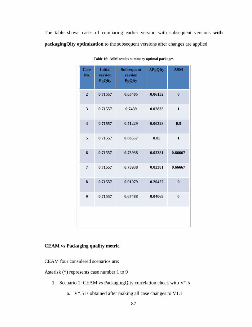
87
The table shows cases of comparing earlier version with subsequent versions with
packagingQlty optimization to the subsequent versions after changes are applied.
Table 16: ASM results summary optimal packages
Case
No.
Initial
version
PgQlty
Subsequent
version
PgQlty
ΔPgQlty ASM
2 0.71557 0.65405 0.06152 0
3 0.71557 0.7439 0.02833 1
4 0.71557 0.71229 0.00328 0.5
5 0.71557 0.66557 0.05 1
6 0.71557 0.73938 0.02381 0.66667
7 0.71557 0.73938 0.02381 0.66667
8 0.71557 0.91979 0.20422 0
9 0.71557 0.67488 0.04069 0
CEAM vs Packaging quality metric
CEAM four considered scenarios are:
Asterisk (*) represents case number 1 to 9
1. Scenario 1: CEAM vs PackagingQlty correlation check with V*.5
a. V*.5 is obtained after making all case changes to V1.1

88
b. optimization is made to the resulting system
c. V*.5 is the best optimal system after changes
2. Scenario 2: CEAM vs PackagingQlty correlation check with V*.6
a. V*.6 is obtained after making all case changes to V1.1
b. optimization is made to the resulting system
c. V*.6 is the second best optimal system after changes
3. Scenario 3: ChangeInCEAM vs ChangeInPackagingQlty correlation check with
V1.2 and V*.2
a. V1.2 is also the optimal configuration of the system
b. That is V1.2 = V1.1
c. V*.2 is obtained after making all case changes to V1.1
d. optimization is made to the resulting system
e. V*.2 is the best optimal system after changes
4. Scenario 4: ChangeInCEAM vs ChangeInPackagingQlty correlation check with
V1.3 and V*.3
a. V1.3 is second best optimal of V1.1
b. V*.3 is obtained after making all case changes to V1.1
c. Optimization is made to the resulting system
d. V*.3 is the second best optimal system after changes
CEAM Results summary: Scenario 1
Table 17 shows case number that indicates hypothetical case version number, PgQlty gives
the packaging quality value of the case version and CEAM gives the CEAM value of the
case version. This was used to compute the correlation which can be visualized on Fig. 39.
The correlation test score for this scenario is 0.41081. The p-value for this correlation test
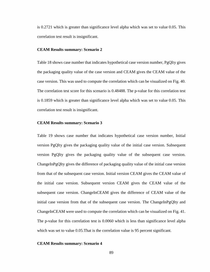
89
is 0.2721 which is greater than significance level alpha which was set to value 0.05. This
correlation test result is insignificant.
CEAM Results summary: Scenario 2
Table 18 shows case number that indicates hypothetical case version number, PgQlty gives
the packaging quality value of the case version and CEAM gives the CEAM value of the
case version. This was used to compute the correlation which can be visualized on Fig. 40.
The correlation test score for this scenario is 0.48488. The p-value for this correlation test
is 0.1859 which is greater than significance level alpha which was set to value 0.05. This
correlation test result is insignificant.
CEAM Results summary: Scenario 3
Table 19 shows case number that indicates hypothetical case version number, Initial
version PgQlty gives the packaging quality value of the initial case version. Subsequent
version PgQlty gives the packaging quality value of the subsequent case version.
ChangeInPgQlty gives the difference of packaging quality value of the initial case version
from that of the subsequent case version. Initial version CEAM gives the CEAM value of
the initial case version. Subsequent version CEAM gives the CEAM value of the
subsequent case version. ChangeInCEAM gives the difference of CEAM value of the
initial case version from that of the subsequent case version. The ChangeInPgQlty and
ChangeInCEAM were used to compute the correlation which can be visualized on Fig. 41.
The p-value for this correlation test is 0.0060 which is less than significance level alpha
which was set to value 0.05.That is the correlation value is 95 percent significant.
CEAM Results summary: Scenario 4
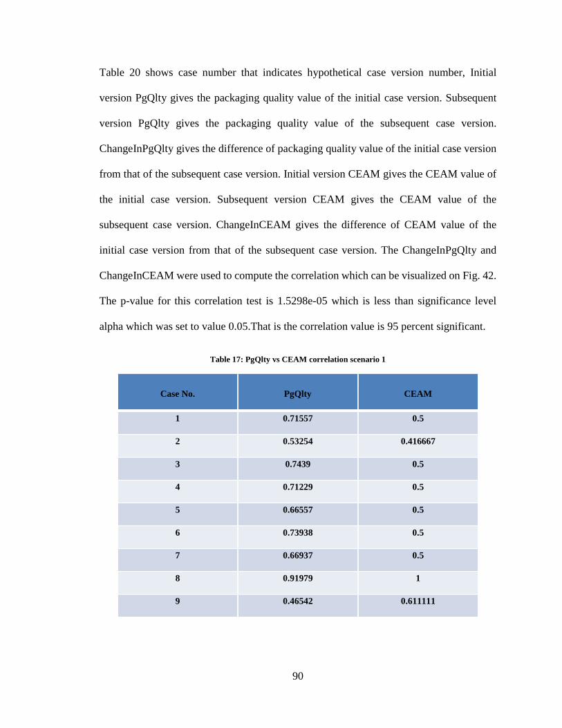
90
Table 20 shows case number that indicates hypothetical case version number, Initial
version PgQlty gives the packaging quality value of the initial case version. Subsequent
version PgQlty gives the packaging quality value of the subsequent case version.
ChangeInPgQlty gives the difference of packaging quality value of the initial case version
from that of the subsequent case version. Initial version CEAM gives the CEAM value of
the initial case version. Subsequent version CEAM gives the CEAM value of the
subsequent case version. ChangeInCEAM gives the difference of CEAM value of the
initial case version from that of the subsequent case version. The ChangeInPgQlty and
ChangeInCEAM were used to compute the correlation which can be visualized on Fig. 42.
The p-value for this correlation test is 1.5298e-05 which is less than significance level
alpha which was set to value 0.05.That is the correlation value is 95 percent significant.
Table 17: PgQlty vs CEAM correlation scenario 1
Case No. PgQlty CEAM
1 0.71557 0.5
2 0.53254 0.416667
3 0.7439 0.5
4 0.71229 0.5
5 0.66557 0.5
6 0.73938 0.5
7 0.66937 0.5
8 0.91979 1
9 0.46542 0.611111
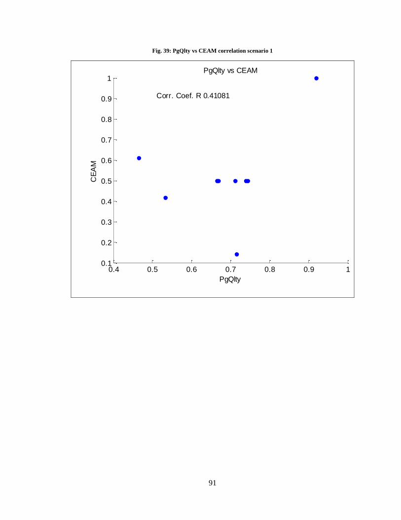
91
Fig. 39: PgQlty vs CEAM correlation scenario 1
0.4 0.5 0.6 0.7 0.8 0.9 10.1
0.2
0.3
0.4
0.5
0.6
0.7
0.8
0.9
1
Corr. Coef. R 0.41081
PgQlty vs CEAM
PgQlty
CE
AM
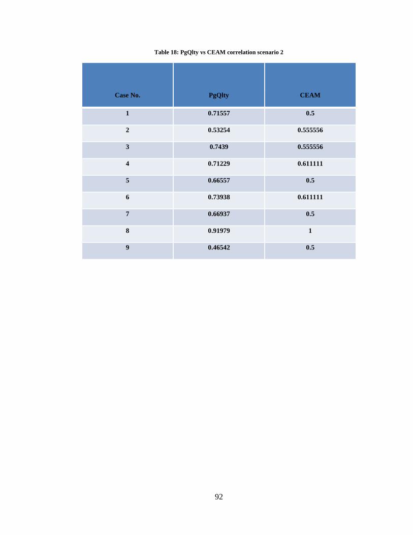
92
Table 18: PgQlty vs CEAM correlation scenario 2
Case No. PgQlty CEAM
1 0.71557 0.5
2 0.53254 0.555556
3 0.7439 0.555556
4 0.71229 0.611111
5 0.66557 0.5
6 0.73938 0.611111
7 0.66937 0.5
8 0.91979 1
9 0.46542 0.5
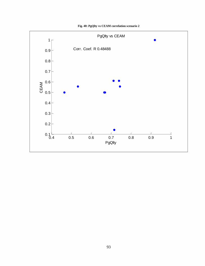
93
Fig. 40: PgQlty vs CEAM correlation scenario 2
0.4 0.5 0.6 0.7 0.8 0.9 10.1
0.2
0.3
0.4
0.5
0.6
0.7
0.8
0.9
1
Corr. Coef. R 0.48488
PgQlty vs CEAM
PgQlty
CE
AM

94
Table 19: ChangeInPgQlty vs ChangeInCEAM correlation scenario 3
Case No. Initial
version
PgQlty
Subsequent
version
PgQlty
ΔPgQlty Initial
version
CEAM
Subsequent
version
CEAM
ΔCEAM
2 0.71557 0.53254 -0.18303 0.5 0.416667 -0.08333
3 0.71557 0.7439 0.02833 0.5 0.5 0
4 0.71557 0.71229 -0.00328 0.5 0.5 0
5 0.71557 0.66557 -0.05 0.5 0.5 0
6 0.71557 0.73938 0.02381 0.5 0.5 0
7 0.71557 0.66937 -0.0462 0.5 0.5 0
8 0.71557 0.91979 0.20422 0.5 1 0.5
9 0.71557 0.46542 -0.25015 0.5 0.611111 0.111111
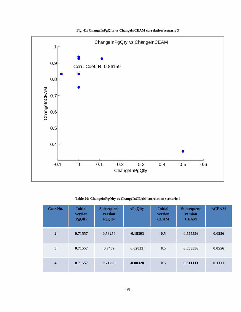
95
Fig. 41: ChangeInPgQlty vs ChangeInCEAM correlation scenario 3
Table 20: ChangeInPgQlty vs ChangeInCEAM correlation scenario 4
Case No. Initial
version
PgQlty
Subsequent
version
PgQlty
ΔPgQlty Initial
version
CEAM
Subsequent
version
CEAM
ΔCEAM
2 0.71557 0.53254 -0.18303 0.5 0.555556 0.0556
3 0.71557 0.7439 0.02833 0.5 0.555556 0.0556
4 0.71557 0.71229 -0.00328 0.5 0.611111 0.1111
-0.1 0 0.1 0.2 0.3 0.4 0.5 0.6
0.4
0.5
0.6
0.7
0.8
0.9
1
Corr. Coef. R -0.86159
ChangeInPgQlty vs ChangeInCEAM
ChangeInPgQlty
Cha
nge
InC
EA
M
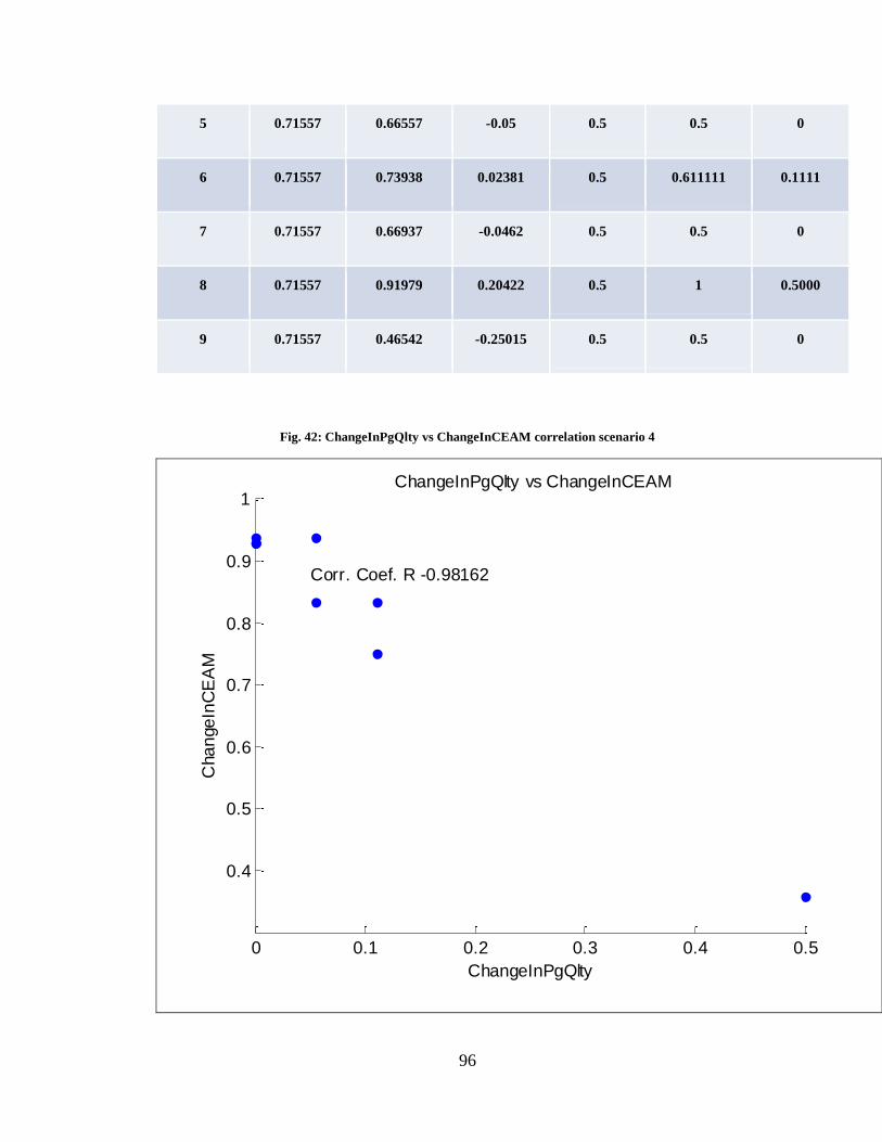
96
5 0.71557 0.66557 -0.05 0.5 0.5 0
6 0.71557 0.73938 0.02381 0.5 0.611111 0.1111
7 0.71557 0.66937 -0.0462 0.5 0.5 0
8 0.71557 0.91979 0.20422 0.5 1 0.5000
9 0.71557 0.46542 -0.25015 0.5 0.5 0
Fig. 42: ChangeInPgQlty vs ChangeInCEAM correlation scenario 4
0 0.1 0.2 0.3 0.4 0.5
0.4
0.5
0.6
0.7
0.8
0.9
1
Corr. Coef. R -0.98162
ChangeInPgQlty vs ChangeInCEAM
ChangeInPgQlty
Cha
nge
InC
EA
M
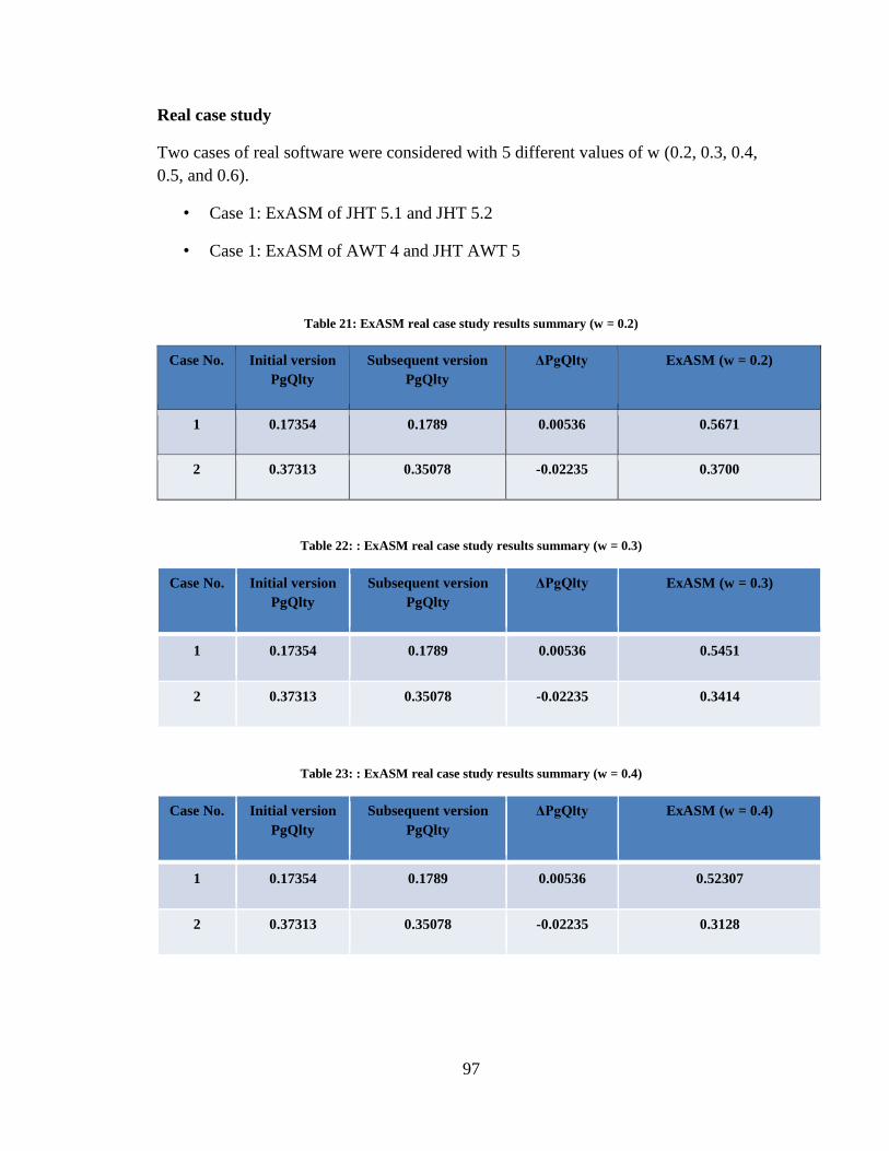
97
Real case study
Two cases of real software were considered with 5 different values of w (0.2, 0.3, 0.4,
0.5, and 0.6).
• Case 1: ExASM of JHT 5.1 and JHT 5.2
• Case 1: ExASM of AWT 4 and JHT AWT 5
Table 21: ExASM real case study results summary (w = 0.2)
Case No. Initial version
PgQlty
Subsequent version
PgQlty
ΔPgQlty ExASM (w = 0.2)
1 0.17354 0.1789 0.00536 0.5671
2 0.37313 0.35078 -0.02235 0.3700
Table 22: : ExASM real case study results summary (w = 0.3)
Case No. Initial version
PgQlty
Subsequent version
PgQlty
ΔPgQlty ExASM (w = 0.3)
1 0.17354 0.1789 0.00536 0.5451
2 0.37313 0.35078 -0.02235 0.3414
Table 23: : ExASM real case study results summary (w = 0.4)
Case No. Initial version
PgQlty
Subsequent version
PgQlty
ΔPgQlty ExASM (w = 0.4)
1 0.17354 0.1789 0.00536 0.52307
2 0.37313 0.35078 -0.02235 0.3128
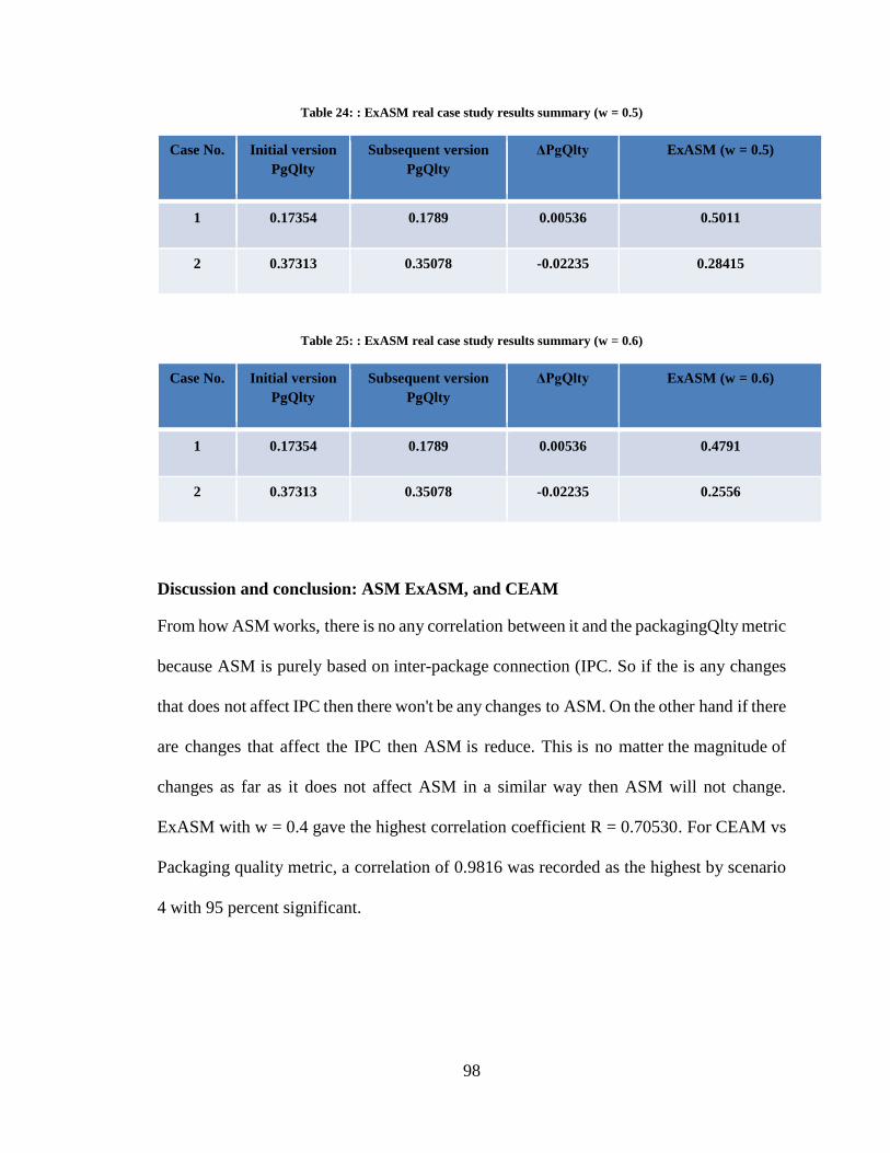
98
Table 24: : ExASM real case study results summary (w = 0.5)
Case No. Initial version
PgQlty
Subsequent version
PgQlty
ΔPgQlty ExASM (w = 0.5)
1 0.17354 0.1789 0.00536 0.5011
2 0.37313 0.35078 -0.02235 0.28415
Table 25: : ExASM real case study results summary (w = 0.6)
Case No. Initial version
PgQlty
Subsequent version
PgQlty
ΔPgQlty ExASM (w = 0.6)
1 0.17354 0.1789 0.00536 0.4791
2 0.37313 0.35078 -0.02235 0.2556
Discussion and conclusion: ASM ExASM, and CEAM
From how ASM works, there is no any correlation between it and the packagingQlty metric
because ASM is purely based on inter-package connection (IPC. So if the is any changes
that does not affect IPC then there won't be any changes to ASM. On the other hand if there
are changes that affect the IPC then ASM is reduce. This is no matter the magnitude of
changes as far as it does not affect ASM in a similar way then ASM will not change.
ExASM with w = 0.4 gave the highest correlation coefficient R = 0.70530. For CEAM vs
Packaging quality metric, a correlation of 0.9816 was recorded as the highest by scenario
4 with 95 percent significant.
99
Hypothesis 3: There is a correlation between the software packaging metric and the
stability metric. This hypothesis can be accepted with the given statistics of CEAM by
scenario 4.
The main challenge with the real case study is that it is still relatively expensive to compute
the metric on it. So it takes a lot of time to run optimization algorithm to find optimal
packaging configuration.
The expectation was that given a software with an initial version v1 packaged with a certain
configuration C1 and after evolution into a new version V2 with configuration C2. If the
difference between the 2 versions packagingQlty is low then ExASM between them should
be high. On the other hand if the difference between the packagingQlty of both version is
high, then the ExASM between them was expected to be low. However the result did not
turn out to support that rational.
PackagingQlty also considers intra-package and inter-package connection among several
many factors as enumerated earlier. However, ExASM is based on just intra-package and
inter-package connections.
Moreover we can look at the investigation in the other way where the packaging metric
actually validates the ExASM metric. That is the ExASM which is based on just changes
intra-package and inter-package connections, may not actually be able to capture the
stronger concept of architectural stability.
Software packaging quality metric from its conception and rational is actually meant to
embody the qualities of software architectural stability metric. Moreover it considers many
other factors that affects software architectural stability. Thus software packaging quality

100
can be seen also as quantification of software stability. Along this line of thought, it will
be easy to see why the ExASM will be inadequate to quantify software stability.
4.4 Optimization algorithms experiment
The solution representation preliminary experiment enable us to get idea of values of
common parameters among the optimization algorithms. It will also let us make a fair and
balanced comparison. Moreover we also take note of algorithm parameters that will not
affect the desired output so that they can be fixed. This will also help rapidly scale down
the number of experiments. The penalized model was used with the model parameters fixed
to what was learned at the model selection experiment stage in section 4.3 Search grid
technique is used to find the parameter values for each algorithm that gives the best output
value. The experiment design earlier was used for this experiment also to further
systematically scale down the number of experiments. The only output measure used to
compare the algorithms of output measures used to evaluate the algorithms
4.4.1 Result optimization algorithms evaluation
The result of experiment of comparing 3 algorithms (GA, CMA-ES, and DE) on the
hypothetical case study is reported below. For each algorithm, a table comprising of
algorithm parameters, instance number (that is a given combination of parameters), average
score from three runs of an instance, and the best score from that instance. The graphical
plot display that shows the performance of the algorithms is captured at the end of the
optimization and depicted below to give a visualization of the performance of each
algorithm. How the graphical plot is interpreted is explained in section 2.2.6.Among all the
algorithms being reported CMA-ES performed better since it has the lowest average scores.
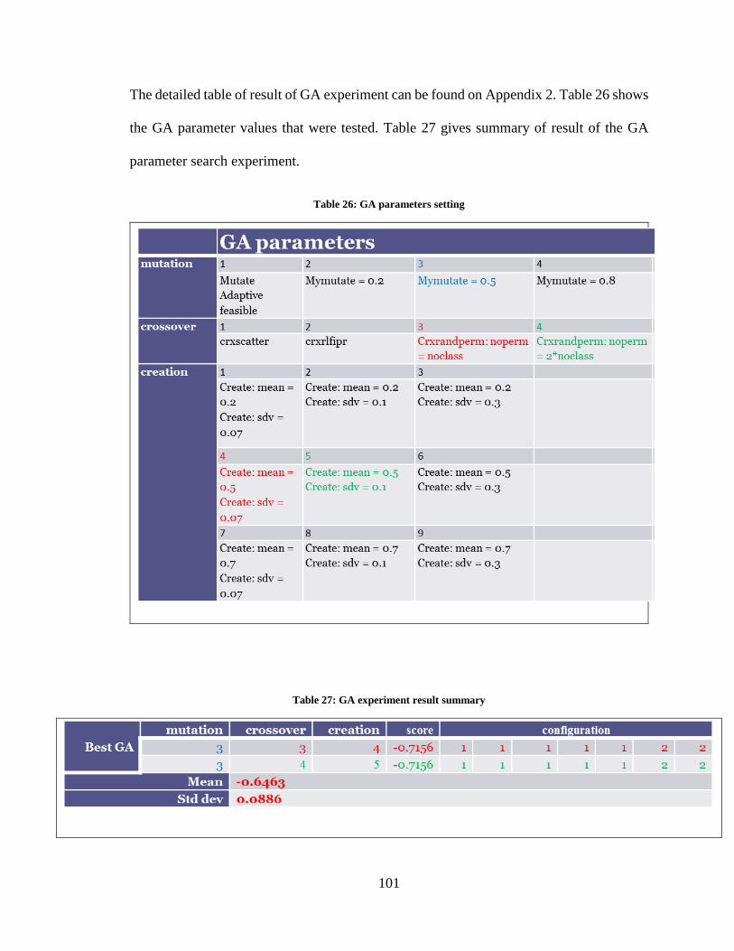
101
The detailed table of result of GA experiment can be found on Appendix 2. Table 26 shows
the GA parameter values that were tested. Table 27 gives summary of result of the GA
parameter search experiment.
Table 26: GA parameters setting
Table 27: GA experiment result summary
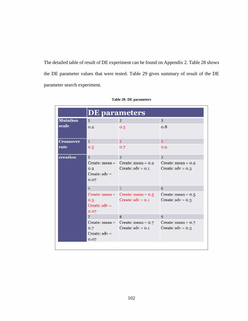
102
The detailed table of result of DE experiment can be found on Appendix 2. Table 28 shows
the DE parameter values that were tested. Table 29 gives summary of result of the DE
parameter search experiment.
Table 28: DE parameters
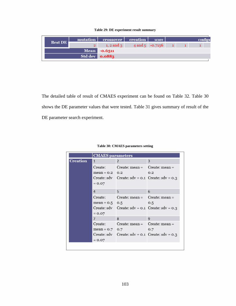
103
Table 29: DE experiment result summary
The detailed table of result of CMAES experiment can be found on Table 32. Table 30
shows the DE parameter values that were tested. Table 31 gives summary of result of the
DE parameter search experiment.
Table 30: CMAES parameters setting
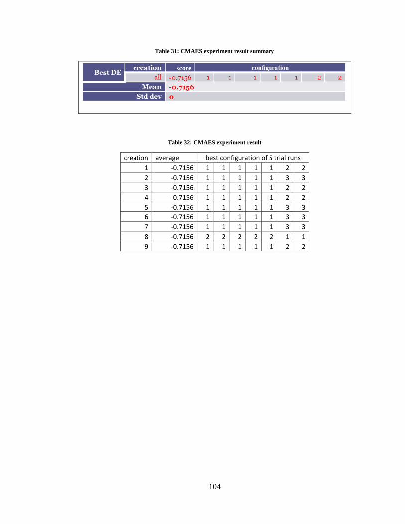
104
Table 31: CMAES experiment result summary
Table 32: CMAES experiment result
creation average best configuration of 5 trial runs
1 -0.7156 1 1 1 1 1 2 2
2 -0.7156 1 1 1 1 1 3 3
3 -0.7156 1 1 1 1 1 2 2
4 -0.7156 1 1 1 1 1 2 2
5 -0.7156 1 1 1 1 1 3 3
6 -0.7156 1 1 1 1 1 3 3
7 -0.7156 1 1 1 1 1 3 3
8 -0.7156 2 2 2 2 2 1 1
9 -0.7156 1 1 1 1 1 2 2
105
5 CHAPTER 5
CONCLUSION
5.1 Contributions and their implications
Steps to be taken to identify, analyze, formulate and solve an optimization (multi or single
objective) problem were clearly outlined. This will serve as a contribution guide for
researcher pursuing this endeavor.
Ways in which an objective function can be formulated were clearly shown. It was shown
clearly the relationship between machine learning and optimization. This will provide help
for new and novice researchers to understand what they mean and how they relate.
A neural network interpretation of the original model was done successfully and the metric
extended thereby. Thus, a path for feature research in automation of quantification and
qualification of software artifacts is shown. This will pave way for applying and
investigating several neural network techniques for packaging software systems.
This way, simple metrics can be acquired to formulate different architecture of neural
networks then train them by using a training and validation dataset.
Consequently, neural network technique can be applied to other software engineering by
acquiring simple software metrics from good knowledge of metrics formulation or simply
by use of metric tools one can be able to develop a model for automatic quantification or
qualification of software artifacts.
106
This study helps to further strengthen and demonstrate the justification and popularity of
neural networks as current state-of-the-art in modeling. We can see that though the original
model was formulated by the designer by handwork and hard work - reasoning through
how simple metrics should be combined to formulate higher level metrics in layer wise
hierarchical manner, and subsequently the desired output was reached. However, the same
desired output (and even better) can be reached by application of neural network techniques
without the hassle of going through manually formulating complicated but necessary
feature need to reach the desired output.
So the lesson is, we should not spend effort formulating latent features that are complicated
(and even incomprehensible that we even run out of how to name them) instead acquire as
many of the direct features as possible and let the neural network learn the higher level
features by itself.
5.2 Threats to validity
5.2.1 Threats to construct validity
To be sure we actually measured what we conceive as software packaging quality, software
projects that have lived long over several evolutions have to be documented.
The notion of architectural stability is a very strong qualitative and abstract concept. One
can debate if the metrics ASM and ExASM are actually able to capture that strong concept.
Because ASM and ExASM where defined based on the assumption that change is reverse
of stability. Stability may entail more than just that.
107
Question may be raised as regard whether metric can actually be referred to as
convolutional neural network (CNN). However, with all conviction and from earlier
authoritative works we can truly refer to the metric as a CNN.
5.2.2 Threats to external validity
The case studies considered will still be considered inadequate to make a true
generalization about the research objective. More studies have to be done with more real
cases to have more statistical significance and to enable more confident conclusion.
5.2.3 Threats to Internal validity
The much training and validation data is usually needed to train and validate neural
network. In this experiment hypothetical case study data and expert suggested
configuration ranking was used as in training and validation of the neural network. This
may be very difficult in real case.
5.3 Future work
Meta-optimization for tuning model and hyper parameters. We could study how effective
meta-optimization could be for this kind of optimization problem. Afterwards, we could
also study how well some optimization algorithm do when used for meta-optimization.
Investigate other outputs attributes of meta-heuristic algorithms and how the correlate with
solutions, the algorithms' parameters and each other. In this case it is a Multi-objective
Meta-optimization of OA.
A more succinct neural network interpretation of the original overallpackaing metric.

108
Creating training and validation dataset using the hypothetical case study configurations
and Spearman rank correlation coefficient ranking as fitness function.
Investigate how the metrics used can be mined from source code and runtime logs. In this
work the metrics are formulated from UCs. Perhaps, there may be already existing source
code and runtime metrics that are correlated with the metrics used in this work.
109
References
[1] H. Abdeen, S. Ducasse, H. Sahraoui, I. Alloui, Automatic Package Coupling and
Cycle Minimization, in: Proc. 2009 16th Work. Conf. Reverse Eng., IEEE Computer
Society, Washington, DC, USA, 2009: pp. 103–112.
[2] M. Ali, M. Pant, A. Abraham, Simplex differential evolution, Acta Polytech.
Hungarica. 6 (2009) 95–115.
[3] A. Alkhalid, M. Alshayeb, S.A. Mahmoud, Software refactoring at the package level
using clustering techniques, IET Softw. 5 (2011) 276–284.
[4] M.H. Alsuwaiyel, Algorithms: Design Techniques and Analysis, World Scientific
Publishing Company Pte Limited, 2016.
[5] L. Aversano, M. Molfetta, M. Tortorella, Evaluating architecture stability of
software projects, in: 2013 20th Work. Conf. Reverse Eng., 2013: pp. 417–424.
[6] S. Bandyopadhyay, S. Saha, Some Single- and Multiobjective Optimization
Techniques BT - Unsupervised Classification: Similarity Measures, Classical and
Metaheuristic Approaches, and Applications, in: S. Bandyopadhyay, S. Saha (Eds.),
Springer Berlin Heidelberg, Berlin, Heidelberg, 2013: pp. 17–58.
[7] J. Bansiya, Evaluating Framework Architecture Structural Stability, ACM Comput.
Surv. 32 (2000) 1–8.
[8] M. Bauer, M. Trifu, Architecture-aware adaptive clustering of OO systems, in:
Eighth Eur. Conf. Softw. Maint. Reengineering, 2004. CSMR 2004. Proceedings.,
IEEE, 2004: pp. 3–14.
[9] A. Ben-Tal, A. Nemirovski, Lectures on Modern Convex Optimization: Analysis,
Algorithms, and Engineering Applications, Society for Industrial and Applied
Mathematics, 2001.
[10] Y.J. Cao, L. Jiang, Q.H. Wu, An evolutionary programming approach to mixed-
variable optimization problems, Appl. Math. Model. 24 (2000) 931–942.
[11] R. Chocat, L. Brevault, M. Balesdent, S. Defoort, Modified Covariance Matrix
Adaptation – Evolution Strategy algorithm for constrained optimization under
uncertainty, application to rocket design, Int. J. Simul. Multidiscip. Des. Optim. 6
(2015) A1.
[12] T.H. Cormen, Introduction to Algorithms, MIT Press, 2009.
[13] K. Deep, K.P. Singh, M.L. Kansal, C. Mohan, A real coded genetic algorithm for
solving integer and mixed integer optimization problems, Appl. Math. Comput. 212
(2009) 505–518.
110
[14] J. Delgrande, W. Faber, Logic Programming and Nonmonotonic Reasoning: 11th
International Conference, LPNMR 2011, Vancouver, Canada, May 16-19, 2011,
Proceedings, Springer Berlin Heidelberg, 2011.
[15] M. Dorigo, M. Birattari, T. Stutzle, Ant colony optimization, IEEE Comput. Intell.
Mag. 1 (2006) 28–39.
[16] D. Doval, S. Mancoridis, B.S.S. Mitchell, Automatic clustering of software systems
using a genetic algorithm, in: STEP ’99. Proc. Ninth Int. Work. Softw. Technol.
Eng. Pract., IEEE Comput. Soc, 1999: pp. 73–81.
[17] L. Duta, F.G. Filip, J.M. Henrioud, A method for dealing with multi-objective
optimization problem of disassembly processes, in: Proc. IEEE Int. Symp.
onAssembly Task Planning, 2003., 2003: pp. 163–168.
[18] S. Ebad, Towards measuring software requirements volatility: A retrospective
analysis, Malaysian J. Comput. Sci. 30 (2017) 99–116.
[19] S.A. Ebad, M.A. Ahmed, Measuring stability of object-oriented software
architectures, IET Softw. 9 (2015) 76–82.
[20] S.A. Ebad, M.A. Ahmed, Functionality-based software packaging using sequence
diagrams, Softw. Qual. J. 23 (2015) 453–481.
[21] S.A. Ebad, M.A. Ahmed, Review and Evaluation of Cohesion and Coupling Metrics
at Package and Subsystem Level, 11 (2016) 598–605.
[22] M.A. Gennert, A.L. Yuille, Determining the optimal weights in multiple objective
function optimization, in: 2nd Int. Conf. Comp. Vis., 1988: pp. 87–89.
[23] Y. Gil, G. Lalouche, On the correlation between size and metric validity, Empir.
Softw. Eng. 22 (2017) 2585–2611.
[24] D. Greiner, B. Galván, J. Périaux, N. Gauger, K. Giannakoglou, G. Winter,
Advances in Evolutionary and Deterministic Methods for Design, Optimization and
Control in Engineering and Sciences, Springer International Publishing, 2014.
[25] R.M. Heiberger, E. Neuwirth, Polynomial Regression BT - R Through Excel: A
Spreadsheet Interface for Statistics, Data Analysis, and Graphics, in: R.M.
Heiberger, E. Neuwirth (Eds.), Springer New York, New York, NY, 2009: pp. 269–
284.
[26] G.E. Hinton, Reducing the Dimensionality of Data with Neural Networks, Science
(80-. ). 313 (2006) 504–507.
[27] M. Jazayeri, On Architectural Stability and Evolution BT - Reliable Software
Technologies — Ada-Europe 2002: 7th Ada-Europe International Conference on
Reliable Software Technologies Vienna, Austria, June 17–21, 2002 Proceedings, in:
J. Blieberger, A. Strohmeier (Eds.), Springer Berlin Heidelberg, Berlin, Heidelberg,
2002: pp. 13–23.
111
[28] I.F. Jr., X.-S. Yang, I. Fister, J. Brest, D. Fister, A Brief Review of Nature-Inspired
Algorithms for Optimization, CoRR. abs/1307.4 (2013).
[29] J. Kennedy, Particle swarm optimization, in: Encycl. Mach. Learn., Springer, 2011:
pp. 760–766.
[30] M. Khajehzadeh, M.R. Taha, A. El-Shafie, M. Eslami, A survey on meta-heuristic
global optimization algorithms, Res. J. Appl. Sci. Eng. Technol. 3 (2011) 569–578.
[31] M. Kokkolaras, C. Audet, J.E. Dennis, Mixed Variable Optimization of the Number
and Composition of Heat Intercepts in a Thermal Insulation System, Optim. Eng. 2
(2001) 5–29.
[32] S. Körkel, H. Qu, G. Rücker, S. Sager, Derivative Based vs. Derivative Free
Optimization Methods for Nonlinear Optimum Experimental Design BT - Current
Trends in High Performance Computing and Its Applications: Proceedings of the
International Conference on High Performance Computing and Appl, in: W. Zhang,
W. Tong, Z. Chen, R. Glowinski (Eds.), Springer Berlin Heidelberg, Berlin,
Heidelberg, 2005: pp. 339–344.
[33] D.C. LeBlanc, Statistics: Concepts and Applications for Science, Jones and Bartlett,
2004.
[34] H.F. Li, W.K. Cheung, An Empirical Study of Software Metrics, IEEE Trans. Softw.
Eng. SE-13 (1987) 697–708.
[35] X. Liu, S. Swift, A. Tucker, Using Evolutionary Algorithms to Tackle Large Scale
Grouping Problems, in: Proc. 3rd Annu. Conf. Genet. Evol. Comput., Morgan
Kaufmann Publishers Inc., San Francisco, CA, USA, 2001: pp. 454–460.
[36] D.T. Luc, Multiobjective Linear Programming: An Introduction, Springer
International Publishing, 2015.
[37] S. Lucidi, V. Piccialli, M. Sciandrone, An Algorithm Model for Mixed Variable
Programming, SIAM J. Optim. 15 (2005) 1057–1084.
[38] C.-H. Lung, X. Xu, M. Zaman, A. Srinivasan, Program restructuring using
clustering techniques, J. Syst. Softw. 79 (2006) 1261–1279.
[39] H. Ma, W. Shao, L. Zhang, Z. Ma, Y. Jiang, Applying OO Metrics to Assess UML
Meta-models BT - «UML» 2004 — The Unified Modeling Language. Modeling
Languages and Applications: 7th International Conference, Lisbon, Portugal,
October 11-15, 2004. Proceedings, in: T. Baar, A. Strohmeier, A. Moreira, S.J.
Mellor (Eds.), Springer Berlin Heidelberg, Berlin, Heidelberg, 2004: pp. 12–26.
[40] H. Ma, D. Simon, Evolutionary Computation with Biogeography-based
Optimization, Wiley, 2017.
[41] S. Mancoridis, B.S. Mitchell, Y. Chen, E.R. Gansner, Bunch: a clustering tool for
the recovery and maintenance of software system structures, in: Proc. IEEE Int.
112
Conf. Softw. Maint. - 1999 (ICSM’99). ’Software Maint. Bus. Chang. (Cat.
No.99CB36360), IEEE, 1999: pp. 50–59.
[42] S. Mancoridis, B.S. Mitchell, C. Rorres, Y. Chen, E.R. Gansner, Using automatic
clustering to produce high-level system organizations of source code, in: Progr.
Comprehension, 1998. IWPC ’98. Proceedings., 6th Int. Work., 1998: pp. 45–52.
[43] R.C. Martin, Agile software development: principles, patterns, and practices,
Prentice Hall, 2002.
[44] N. Medvidovic, R.N. Taylor, Software architecture: foundations, theory, and
practice, in: Proc. 32nd ACM/IEEE Int. Conf. Softw. Eng. 2, 2010: pp. 471–472.
[45] A. Migdalas, P.M. Pardalos, P. Värbrand, Multilevel Optimization: Algorithms and
Applications, Springer US, 2013.
[46] B.S. Mitchell, S. Mancoridis, Using Heuristic Search Techniques To Extract Design
Abstractions From Source Code, in: Proc. Genet. Evol. Comput. Conf., Morgan
Kaufmann Publishers Inc., 2002: pp. 1375–1382.
[47] M. Mitchell, An introduction to genetic algorithms Cambridge, MA, (1998).
[48] M. Mitchell, An Introduction to Genetic Algorithms, MIT Press, Cambridge, MA,
USA, 1998.
[49] G.L. Nemhauser, L.A.B.T.-H. in O.R. and M.S. Wolsey, Chapter VI Integer
programming, in: Optimization, Elsevier, 1989: pp. 447–527.
[50] C.H. Papadimitriou, K. Steiglitz, Combinatorial Optimization: Algorithms and
Complexity, Dover Publications, 2013.
[51] R.E. Perez, K. Behdinan, Particle swarm approach for structural design
optimization, Comput. Struct. 85 (2007) 1579–1588.
[52] F. Rothlauf, Optimization Problems BT - Design of Modern Heuristics: Principles
and Application, in: F. Rothlauf (Ed.), Springer Berlin Heidelberg, Berlin,
Heidelberg, 2011: pp. 7–44.
[53] W.S. Sarle, Neural Networks and Statistical Models, (1994).
[54] G.A.F. Seber, A.J. Lee, Polynomial Regression, in: Linear Regres. Anal., John
Wiley & Sons, Inc., 2003: pp. 165–185.
[55] O. Seng, M. Bauer, M. Biehl, G. Pache, Search-based Improvement of Subsystem
Decompositions, in: Proc. 7th Annu. Conf. Genet. Evol. Comput., ACM, New York,
NY, USA, 2005: pp. 1045–1051.
[56] D. Simon, Evolutionary Optimization Algorithms, Wiley, 2013.
[57] E. Stensrud, T. Foss, B. Kitchenham, I. Myrtveit, A further empirical investigation
of the relationship between MRE and project size, Empir. Softw. Eng. 8 (2003) 139–
113
161.
[58] R. Storn, K. Price, Differential Evolution – A Simple and Efficient Heuristic for
global Optimization over Continuous Spaces, J. Glob. Optim. 11 (1997) 341–359.
[59] B.S. Thomson, J.B. Bruckner, A.M. Bruckner, Elementary Real Analysis, Second
Edition, www.classicalrealanalysis.com., 2008.
[60] S.A. Tonu, A. Ashkan, L. Tahvildari, Evaluating architectural stability using a
metric-based approach, in: Conf. Softw. Maint. Reengineering, 2006: p. 10 pp.-
pp.270.
[61] R.V. V Vidal, Applied Simulated Annealing, Springer Berlin Heidelberg, 2012.
[62] B. Walczak, D.L. Massart, The Radial Basis Functions — Partial Least Squares
approach as a flexible non-linear regression technique, Anal. Chim. Acta. 331
(1996) 177–185.
[63] T. Weise, M. Zapf, R. Chiong, A.J. Nebro, Why Is Optimization Difficult? BT -
Nature-Inspired Algorithms for Optimisation, in: R. Chiong (Ed.), Springer Berlin
Heidelberg, Berlin, Heidelberg, 2009: pp. 1–50.
[64] D.P. Williamson, D.B. Shmoys, The Design of Approximation Algorithms,
Cambridge University Press, 2011.
[65] M.Z. Zakaria, H. Jamaluddin, R. Ahmad, S.M.R. Loghmanian, Comparison between
multi-objective and single-objective optimization for the modeling of dynamic
systems, Proc. Inst. Mech. Eng. Part I J. Syst. Control Eng. 226 (2012) 994–1005.
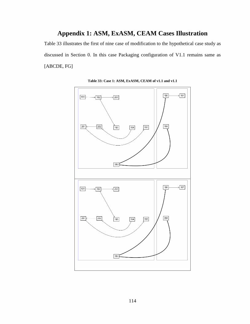
114
Appendix 1: ASM, ExASM, CEAM Cases Illustration
Table 33 illustrates the first of nine case of modification to the hypothetical case study as
discussed in Section 0. In this case Packaging configuration of V1.1 remains same as
[ABCDE, FG]
Table 33: Case 1: ASM, ExASM, CEAM of v1.1 and v1.1
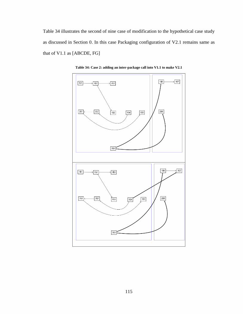
115
Table 34 illustrates the second of nine case of modification to the hypothetical case study
as discussed in Section 0. In this case Packaging configuration of V2.1 remains same as
that of V1.1 as [ABCDE, FG]
Table 34: Case 2: adding an inter-package call into V1.1 to make V2.1
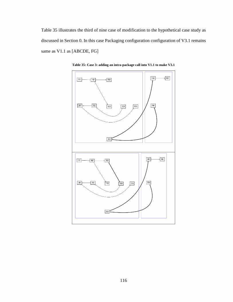
116
Table 35 illustrates the third of nine case of modification to the hypothetical case study as
discussed in Section 0. In this case Packaging configuration configuration of V3.1 remains
same as V1.1 as [ABCDE, FG]
Table 35: Case 3: adding an intra-package call into V1.1 to make V3.1
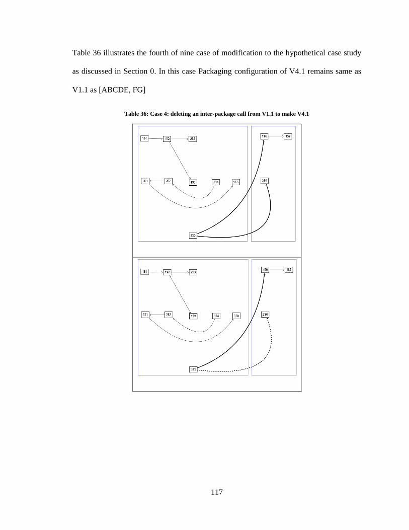
117
Table 36 illustrates the fourth of nine case of modification to the hypothetical case study
as discussed in Section 0. In this case Packaging configuration of V4.1 remains same as
V1.1 as [ABCDE, FG]
Table 36: Case 4: deleting an inter-package call from V1.1 to make V4.1
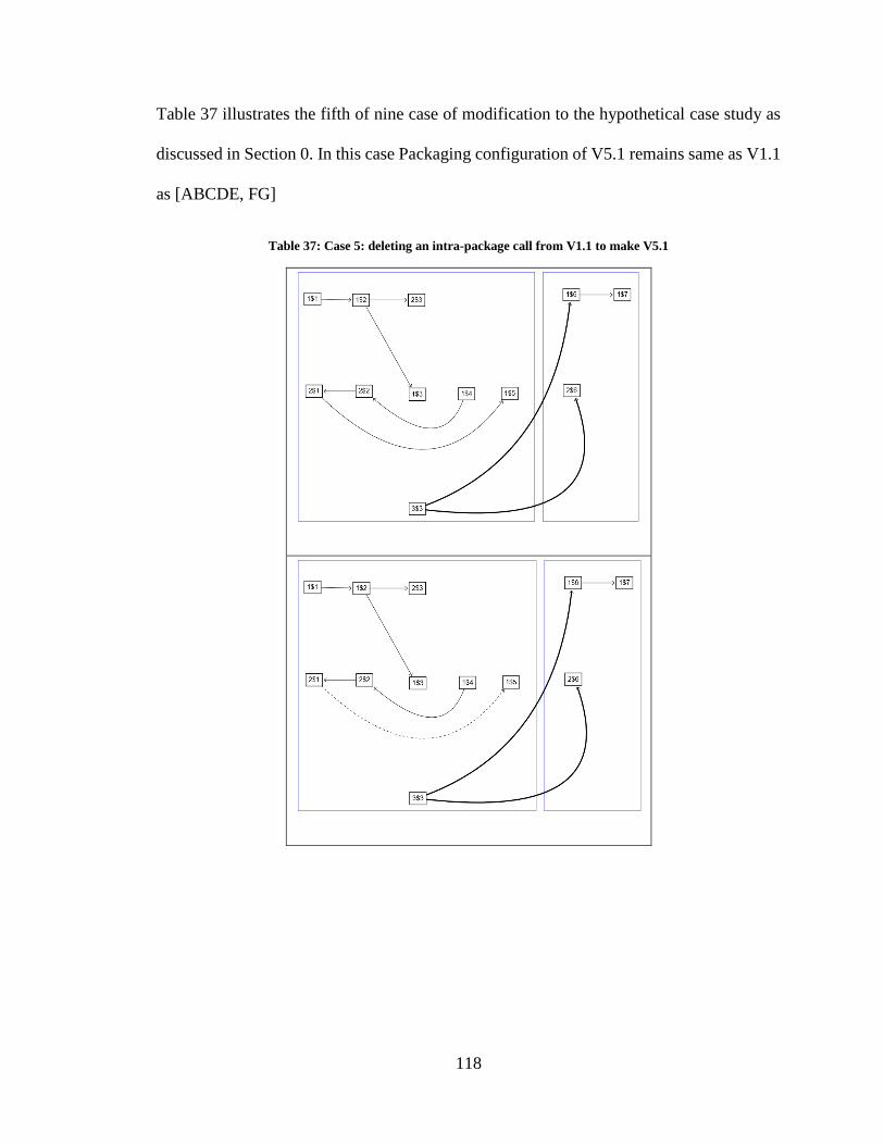
118
Table 37 illustrates the fifth of nine case of modification to the hypothetical case study as
discussed in Section 0. In this case Packaging configuration of V5.1 remains same as V1.1
as [ABCDE, FG]
Table 37: Case 5: deleting an intra-package call from V1.1 to make V5.1
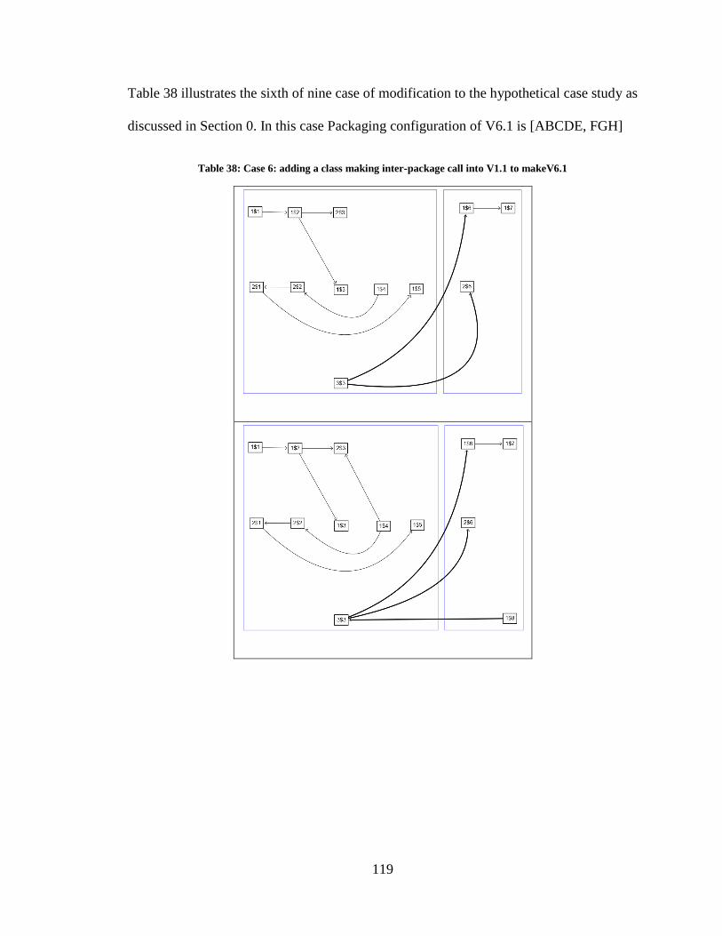
119
Table 38 illustrates the sixth of nine case of modification to the hypothetical case study as
discussed in Section 0. In this case Packaging configuration of V6.1 is [ABCDE, FGH]
Table 38: Case 6: adding a class making inter-package call into V1.1 to makeV6.1
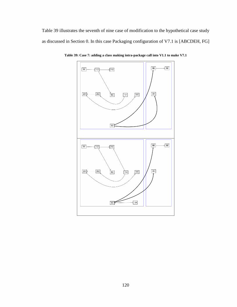
120
Table 39 illustrates the seventh of nine case of modification to the hypothetical case study
as discussed in Section 0. In this case Packaging configuration of V7.1 is [ABCDEH, FG]
Table 39: Case 7: adding a class making intra-package call into V1.1 to make V7.1
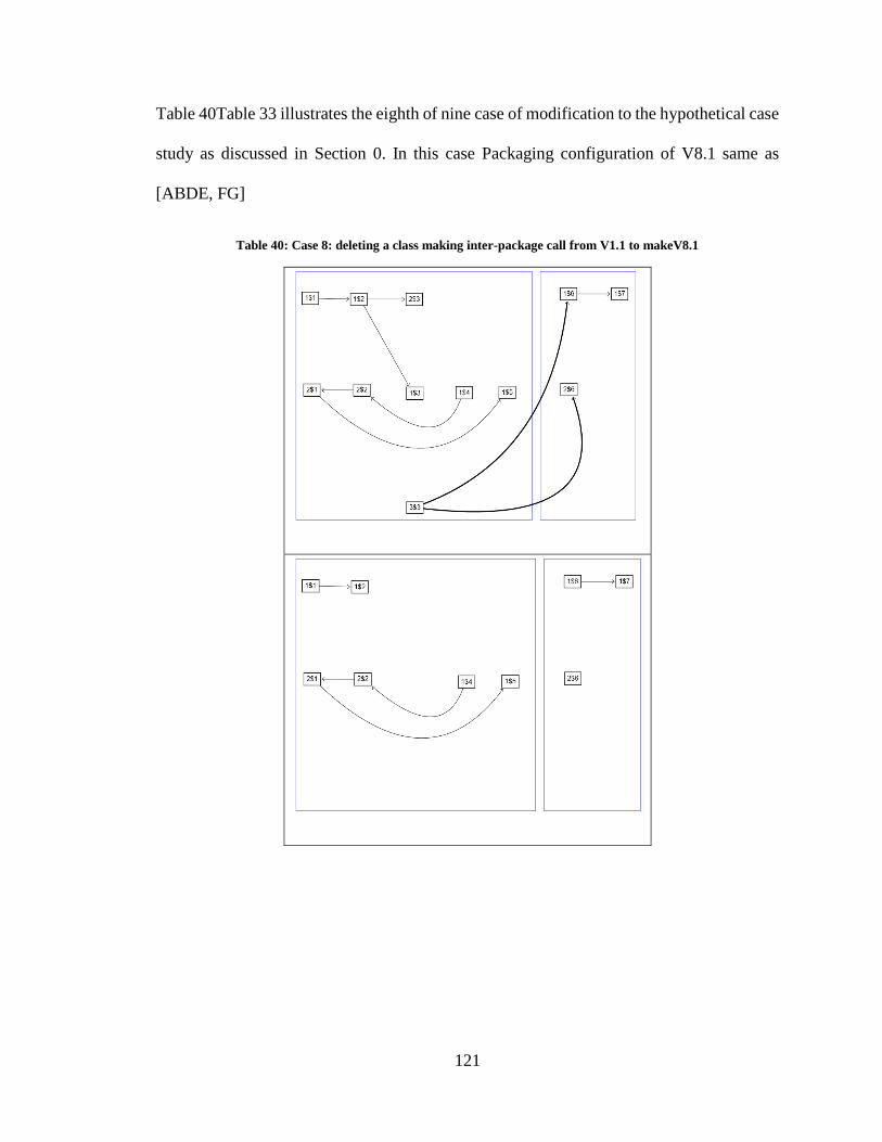
121
Table 40Table 33 illustrates the eighth of nine case of modification to the hypothetical case
study as discussed in Section 0. In this case Packaging configuration of V8.1 same as
[ABDE, FG]
Table 40: Case 8: deleting a class making inter-package call from V1.1 to makeV8.1
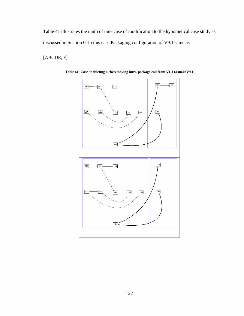
122
Table 41 illustrates the ninth of nine case of modification to the hypothetical case study as
discussed in Section 0. In this case Packaging configuration of V9.1 same as
[ABCDE, F]
Table 41: Case 9: deleting a class making intra-package call from V1.1 to makeV9.1
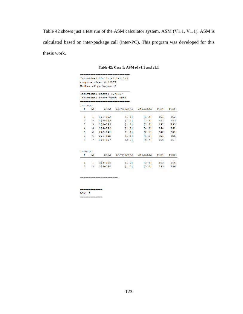
123
Table 42 shows just a test run of the ASM calculator system. ASM (V1.1, V1.1). ASM is
calculated based on inter-package call (inter-PC). This program was developed for this
thesis work.
Table 42: Case 1: ASM of v1.1 and v1.1

124
Table 43 shows just a test run of the ExASM calculator system. ExASM(V1.1, V1.1, 0.4).
ExASM is based on both Intra-package connection and Inter-package connection. This
program was developed for this thesis work.
Table 43: Case 1: ExASM of v1.1 and v1.1
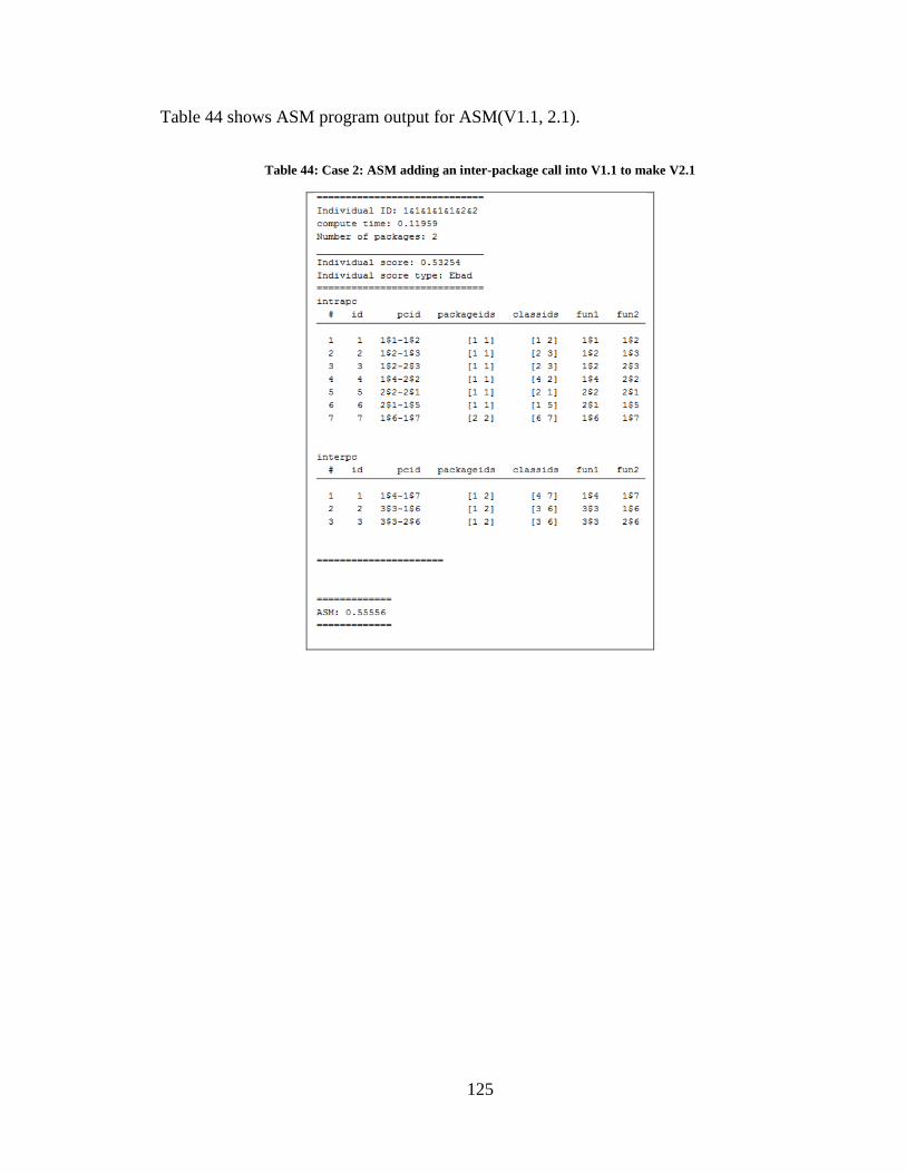
125
Table 44 shows ASM program output for ASM(V1.1, 2.1).
Table 44: Case 2: ASM adding an inter-package call into V1.1 to make V2.1
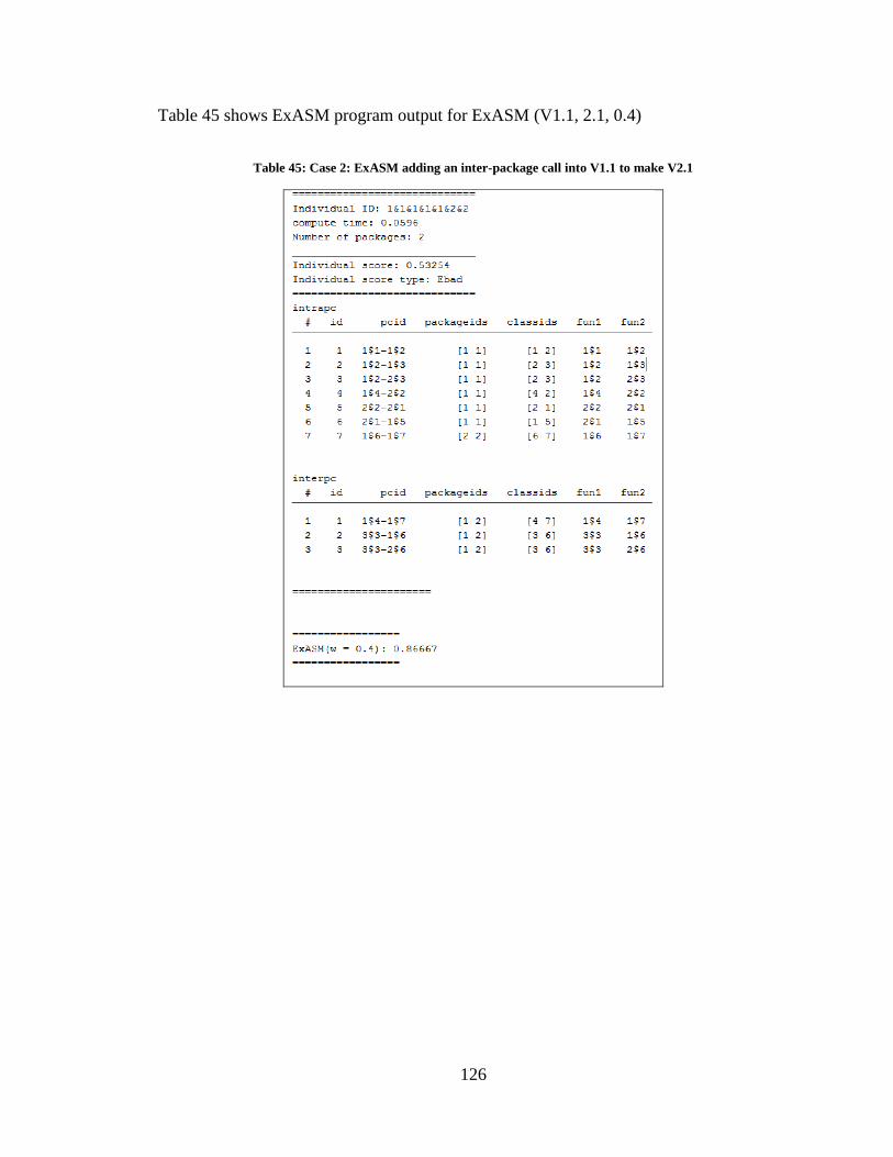
126
Table 45 shows ExASM program output for ExASM (V1.1, 2.1, 0.4)
Table 45: Case 2: ExASM adding an inter-package call into V1.1 to make V2.1

127
Table 46 and Table 47 shows Case 2: Top 2 configurations of V1.1 and V2.1 after
optimization search as (V1.2, V1.3) and (V2.2, V2.3). Note V1.2 = V1.1 since V1.1 is the
top most configuration [1 1 1 1 1 2 2] ([ABCDE, FG]). V1.3 is [1 1 2 1 1 2 2] ([ABDE,
CFG]). V2.2 is supposed to be [1 1 1 1 1 1 1] ([ABCDEFG]) with Ebad score 0.73016. But
this is not a desired configuration. So the next top is taken as V2.2 with [1 1 1 2 2 1 1]
([ABCFG, DE]) with score 0.65405. V2.3 is [1 1 2 3 3 2 2] ([AB, CFG, DE]) with Ebad
score 0.6195
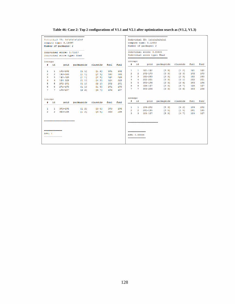
128
Table 46: Case 2: Top 2 configurations of V1.1 and V2.1 after optimization search as (V1.2, V1.3)
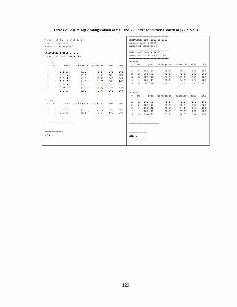
129
Table 47: Case 2: Top 2 configurations of V1.1 and V2.1 after optimization search as (V2.2, V2.3)

130
Table 48 shows ASM program output for ASM (V1.1, 3.1)
Table 48: Case 3: ASM adding an additional intra-package call into V1.1 to make V3.1
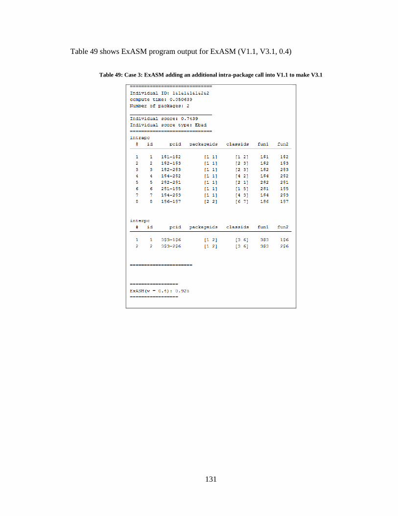
131
Table 49 shows ExASM program output for ExASM (V1.1, V3.1, 0.4)
Table 49: Case 3: ExASM adding an additional intra-package call into V1.1 to make V3.1

132
Table 50 and Table 51 shows Case 3: Top 2 configurations of V1.1 and V3.1 after
optimization search as (V1.2, V1.3) and (V3.2, V3.3). Note V1.2 = V1.1 since V1.1 is the
top most configuration [1 1 1 1 1 2 2] ([ABCDE, FG]). V1.3 is [1 1 2 1 1 2 2] ([ABDE,
CFG]). V3.2 is [1 1 1 1 1 2 2] ([ABCDE, FG]) with score 0.7439. V3.3 is supposed to be
[1 1 1 1 1 1 1] ([ABCDEFG]) with Ebad score 0.73016. But this is not a desired
configuration. So the next top is taken as V3.3 with [1 1 1 2 2 3 3] ([ABC, DE, FG]) with
Ebad score 0.71243.
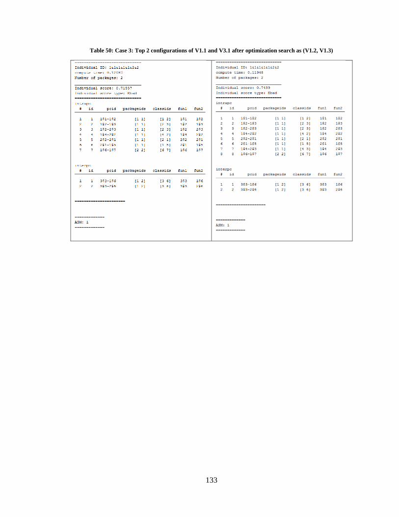
133
Table 50: Case 3: Top 2 configurations of V1.1 and V3.1 after optimization search as (V1.2, V1.3)
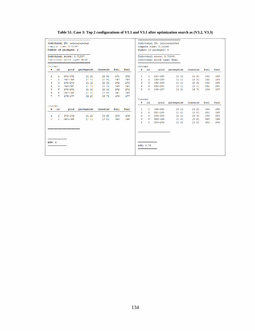
134
Table 51: Case 3: Top 2 configurations of V1.1 and V3.1 after optimization search as (V3.2, V3.3)
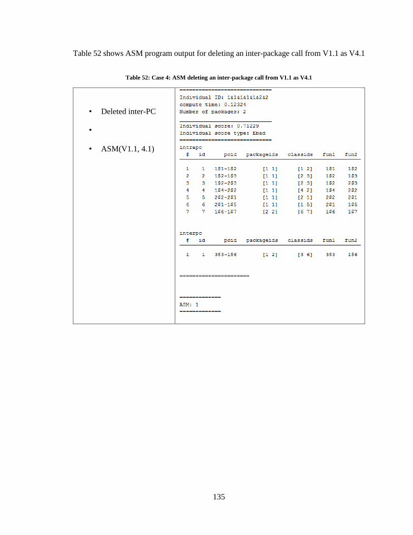
135
Table 52 shows ASM program output for deleting an inter-package call from V1.1 as V4.1
Table 52: Case 4: ASM deleting an inter-package call from V1.1 as V4.1
• Deleted inter-PC
•
• ASM(V1.1, 4.1)
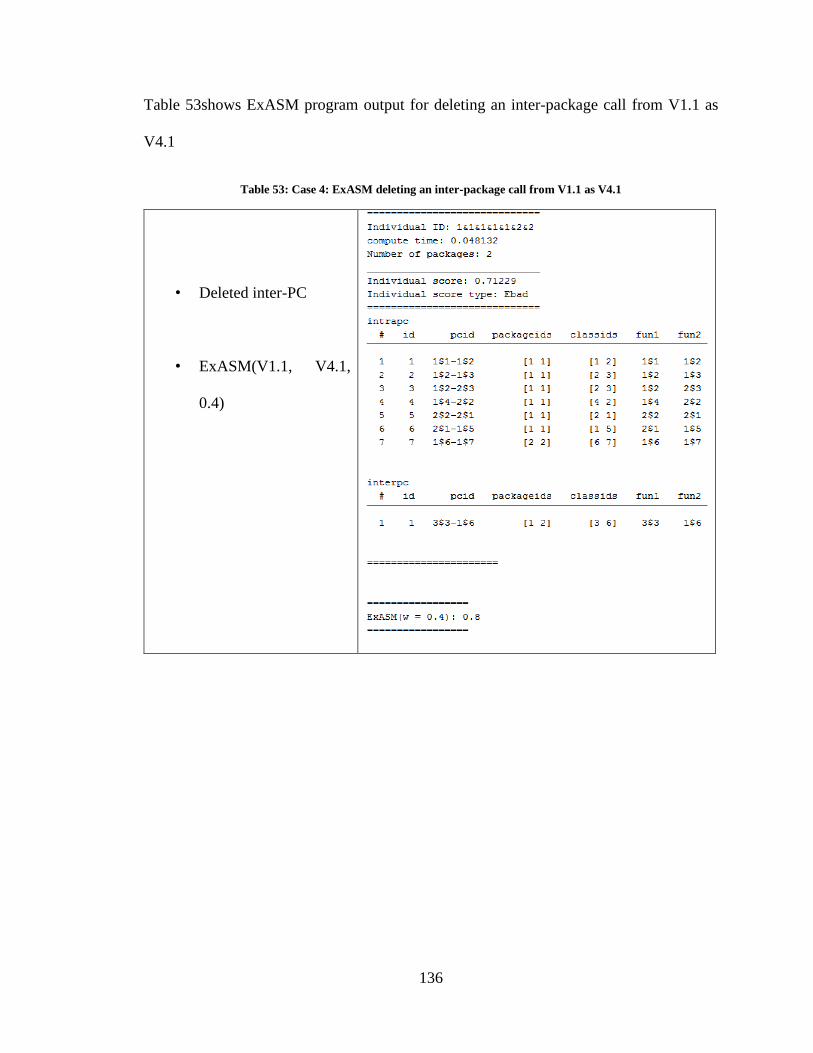
136
Table 53shows ExASM program output for deleting an inter-package call from V1.1 as
V4.1
Table 53: Case 4: ExASM deleting an inter-package call from V1.1 as V4.1
• Deleted inter-PC
• ExASM(V1.1, V4.1,
0.4)

137
Table 54 and Table 55 shows Case 4: Top 2 configurations of V1.1 and V4.1 after
optimization search as (V1.2, V1.3) and (V4.2, V4.3). Note V1.2 = V1.1 since V1.1 is the
top most configuration [1 1 1 1 1 2 2] ([ABCDE, FG]). V1.3 is [1 1 2 1 1 2 2] ([ABDE,
CFG]). V4.2 is [1 1 1 1 1 2 2] ([ABCDE, FG]) with Ebad score 0.71229. [2 2 3 4 4 3 3].
V4.3 is [1 1 2 3 3 2 2] ([ABDE, CFG]) with Ebad score 0.69711.
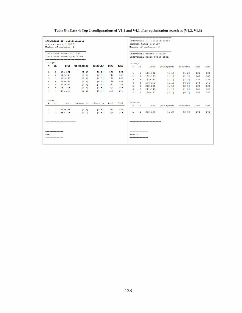
138
Table 54: Case 4: Top 2 configurations of V1.1 and V4.1 after optimization search as (V1.2, V1.3)
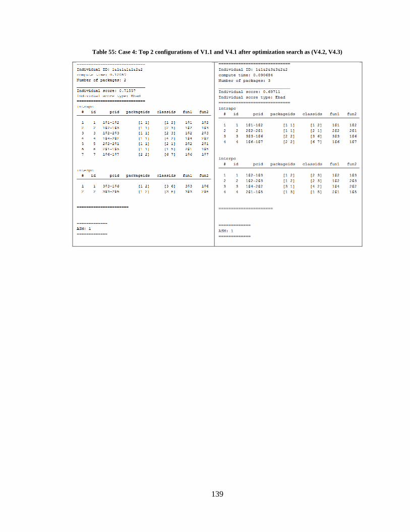
139
Table 55: Case 4: Top 2 configurations of V1.1 and V4.1 after optimization search as (V4.2, V4.3)
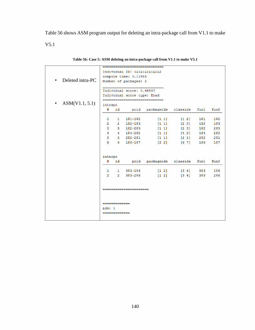
140
Table 56 shows ASM program output for deleting an intra-package call from V1.1 to make
V5.1
Table 56: Case 5: ASM deleting an intra-package call from V1.1 to make V5.1
• Deleted intra-PC
• ASM(V1.1, 5.1)
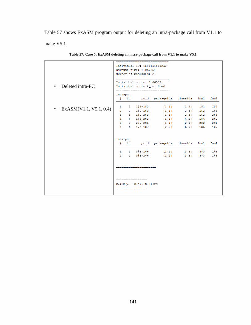
141
Table 57 shows ExASM program output for deleting an intra-package call from V1.1 to
make V5.1
Table 57: Case 5: ExASM deleting an intra-package call from V1.1 to make V5.1
• Deleted intra-PC
• ExASM(V1.1, V5.1, 0.4)

142
Table 58 and Table 59 shows Case 5: Top 2 configurations of V1.1 and V5.1 after
optimization search as (V1.2, V1.3) and (V5.2, V5.3). Note V1.2 = V1.1 since V1.1 is the
top most configuration [1 1 1 1 1 2 2] ([ABCDE, FG]). V1.3 is [1 1 2 1 1 2 2] ([ABDE,
CFG]). V5.2 is [1 1 1 1 1 2 2] ([ABCDE, FG]) with Ebad score 0.66557. V5.3 is supposed
to be [1 1 1 1 1 1 1] ([ABCDEFG]) with Ebad score 0.6587. But this is not a desired
configuration. V5.3 is [1 1 2 1 2 2 2] ([ABDE, CFG]) with Ebad score 0.62344
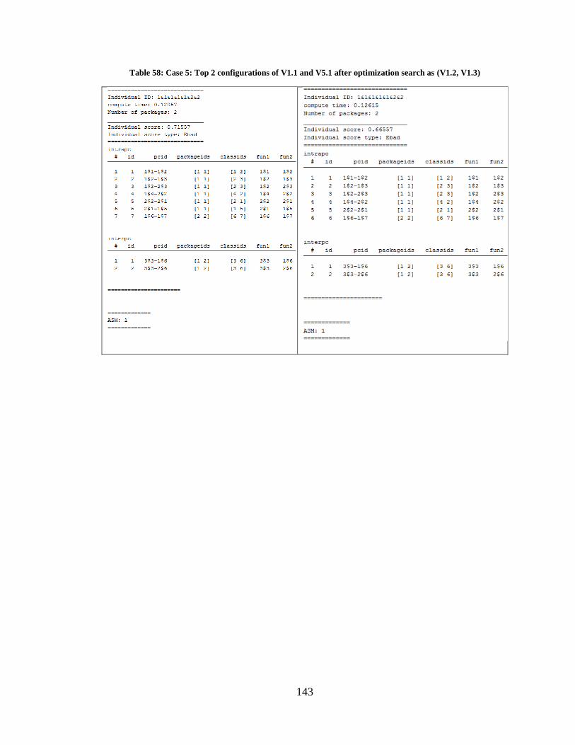
143
Table 58: Case 5: Top 2 configurations of V1.1 and V5.1 after optimization search as (V1.2, V1.3)
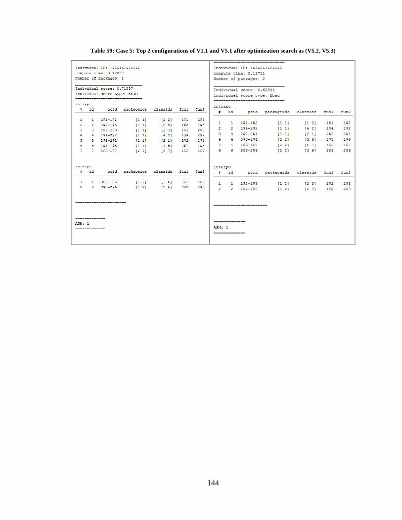
144
Table 59: Case 5: Top 2 configurations of V1.1 and V5.1 after optimization search as (V5.2, V5.3)
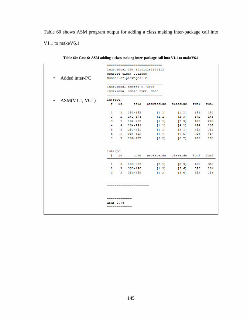
145
Table 60 shows ASM program output for adding a class making inter-package call into
V1.1 to makeV6.1
Table 60: Case 6: ASM adding a class making inter-package call into V1.1 to makeV6.1
• Added inter-PC
• ASM(V1.1, V6.1)
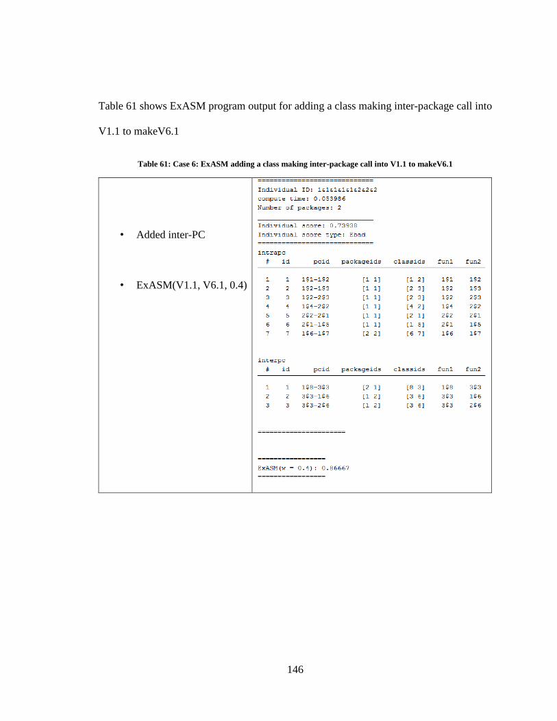
146
Table 61 shows ExASM program output for adding a class making inter-package call into
V1.1 to makeV6.1
Table 61: Case 6: ExASM adding a class making inter-package call into V1.1 to makeV6.1
• Added inter-PC
• ExASM(V1.1, V6.1, 0.4)
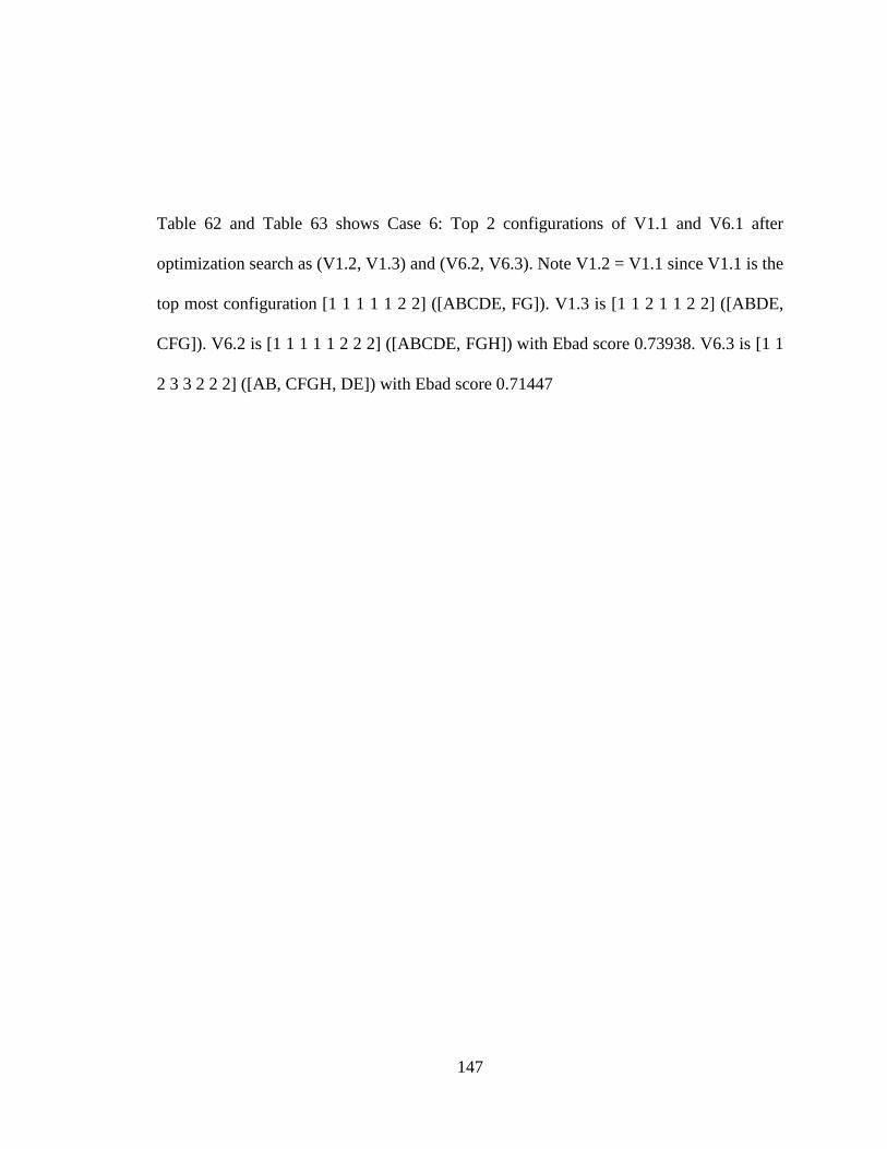
147
Table 62 and Table 63 shows Case 6: Top 2 configurations of V1.1 and V6.1 after
optimization search as (V1.2, V1.3) and (V6.2, V6.3). Note V1.2 = V1.1 since V1.1 is the
top most configuration [1 1 1 1 1 2 2] ([ABCDE, FG]). V1.3 is [1 1 2 1 1 2 2] ([ABDE,
CFG]). V6.2 is [1 1 1 1 1 2 2 2] ([ABCDE, FGH]) with Ebad score 0.73938. V6.3 is [1 1
2 3 3 2 2 2] ([AB, CFGH, DE]) with Ebad score 0.71447
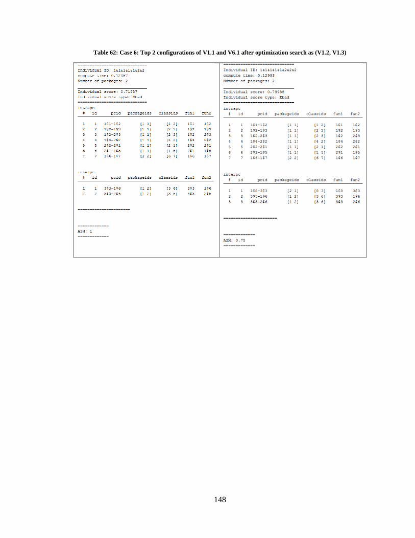
148
Table 62: Case 6: Top 2 configurations of V1.1 and V6.1 after optimization search as (V1.2, V1.3)
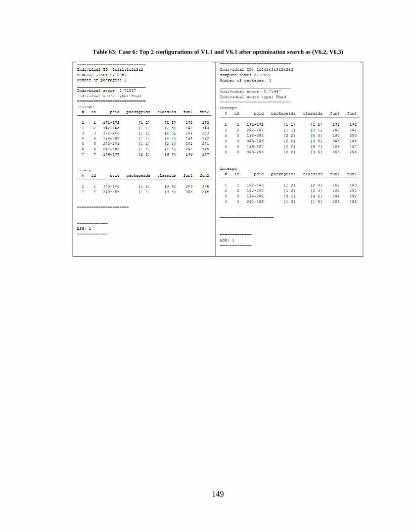
149
Table 63: Case 6: Top 2 configurations of V1.1 and V6.1 after optimization search as (V6.2, V6.3)
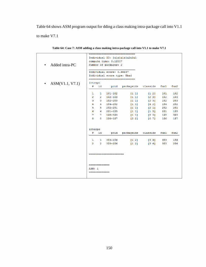
150
Table 64 shows ASM program output for dding a class making intra-package call into V1.1
to make V7.1
Table 64: Case 7: ASM adding a class making intra-package call into V1.1 to make V7.1
• Added intra-PC
• ASM(V1.1, V7.1)

151
Table 65 shows ExASM program output for adding a class making intra-package call into
V1.1 to make V7.1
Table 65: Case 7: ExASM adding a class making intra-package call into V1.1 to make V7.1
• Added intra-PC
• ExASM(V1.1, V7.1, 0.4)
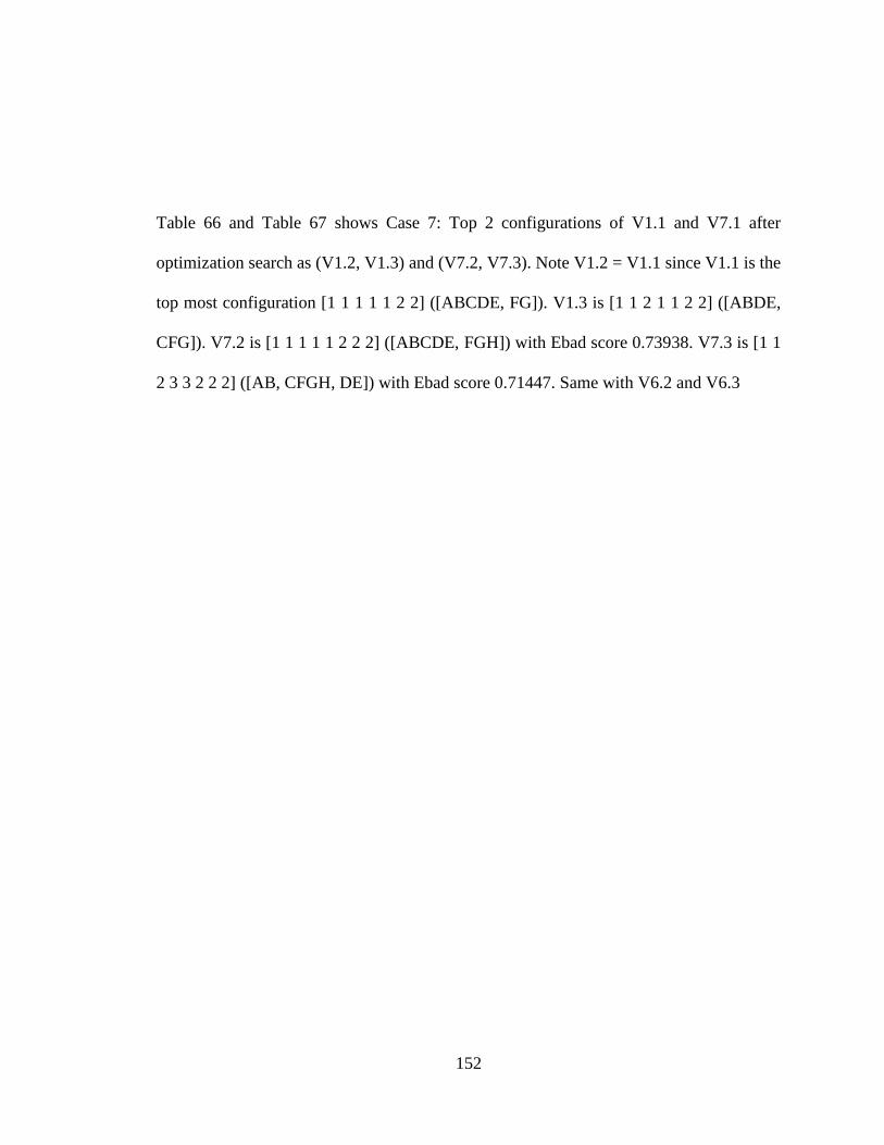
152
Table 66 and Table 67 shows Case 7: Top 2 configurations of V1.1 and V7.1 after
optimization search as (V1.2, V1.3) and (V7.2, V7.3). Note V1.2 = V1.1 since V1.1 is the
top most configuration [1 1 1 1 1 2 2] ([ABCDE, FG]). V1.3 is [1 1 2 1 1 2 2] ([ABDE,
CFG]). V7.2 is [1 1 1 1 1 2 2 2] ([ABCDE, FGH]) with Ebad score 0.73938. V7.3 is [1 1
2 3 3 2 2 2] ([AB, CFGH, DE]) with Ebad score 0.71447. Same with V6.2 and V6.3
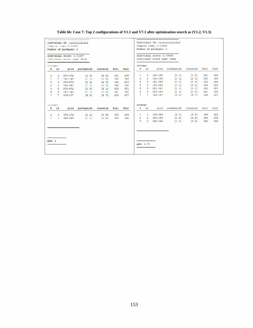
153
Table 66: Case 7: Top 2 configurations of V1.1 and V7.1 after optimization search as (V1.2, V1.3)

154
Table 67: Case 7: Top 2 configurations of V1.1 and V7.1 after optimization search as (V7.2, V7.3)
155
Table 68 shows ASM program output for deleting a class making inter-package call from
V1.1 to makeV8.1
Table 68: Case 8: ASM deleting a class making inter-package call from V1.1 to makeV8.1
• Deleting inter-PC
• ASM(V1.1, V8.1)
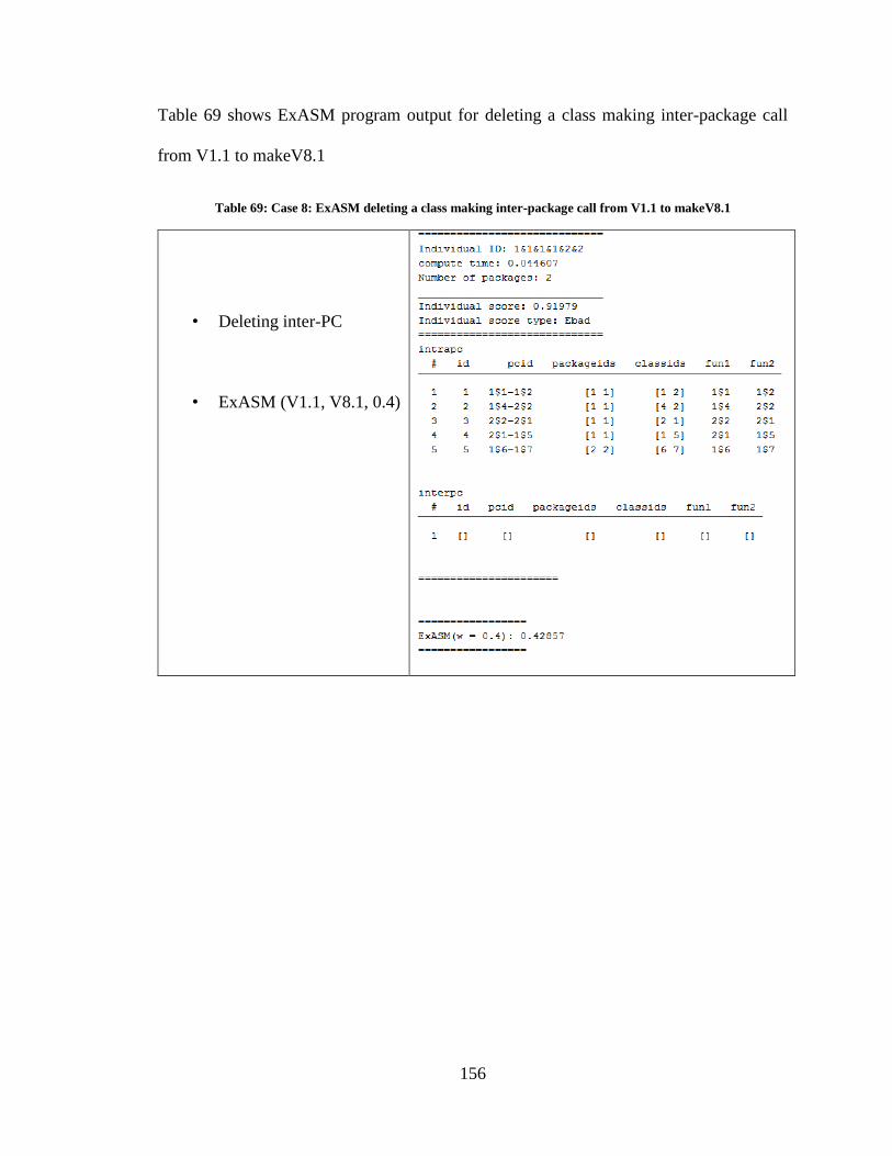
156
Table 69 shows ExASM program output for deleting a class making inter-package call
from V1.1 to makeV8.1
Table 69: Case 8: ExASM deleting a class making inter-package call from V1.1 to makeV8.1
• Deleting inter-PC
• ExASM (V1.1, V8.1, 0.4)

157
Table 70 and Table 71 shows Case 8: Top 2 configurations of V1.1 and V6.1 after
optimization search as (V1.2, V1.3) and (V8.2, V8.3). Note V1.2 = V1.1 since V1.1 is the
top most configuration [1 1 1 1 1 2 2] ([ABCDE,FG]). V1.3 is [1 1 2 1 1 2 2]
([ABDE,CFG]). V8.2 is [1 1 1 1 2 2] ([ABDE, FG]) with Ebad score 0.91979. V8.3 is [1
1 2 2 3 3] ([AB, CD, EF]) with Ebad score 0.84676.
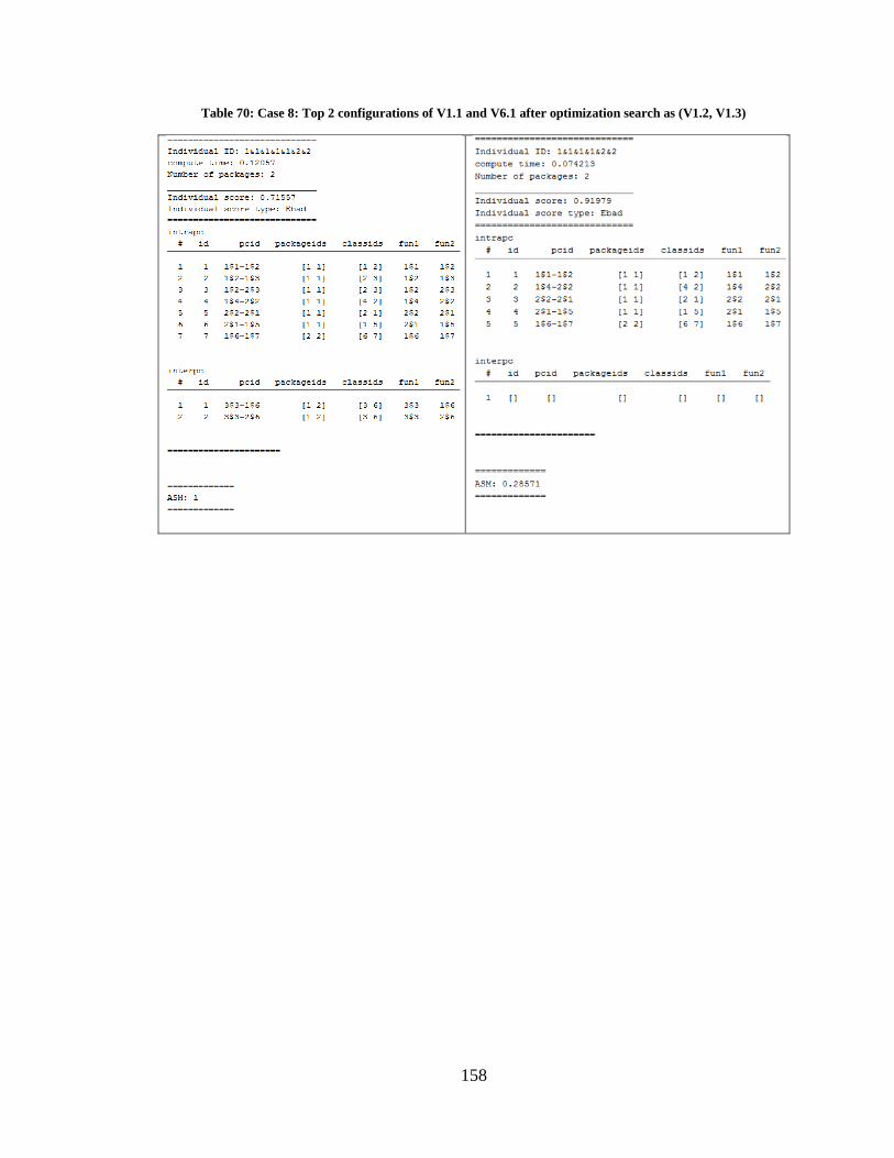
158
Table 70: Case 8: Top 2 configurations of V1.1 and V6.1 after optimization search as (V1.2, V1.3)
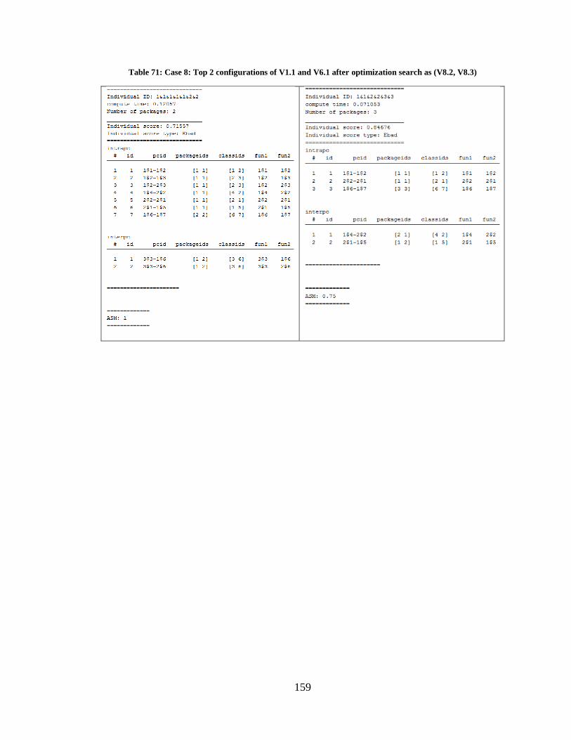
159
Table 71: Case 8: Top 2 configurations of V1.1 and V6.1 after optimization search as (V8.2, V8.3)
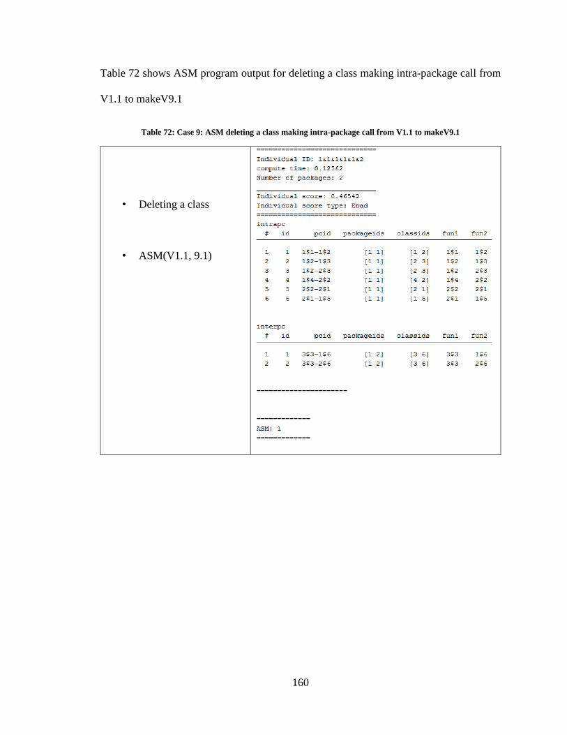
160
Table 72 shows ASM program output for deleting a class making intra-package call from
V1.1 to makeV9.1
Table 72: Case 9: ASM deleting a class making intra-package call from V1.1 to makeV9.1
• Deleting a class
• ASM(V1.1, 9.1)
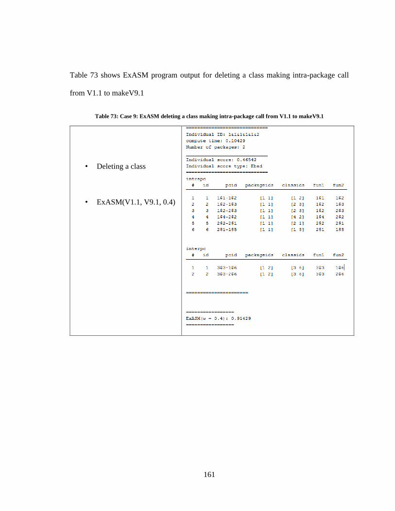
161
Table 73 shows ExASM program output for deleting a class making intra-package call
from V1.1 to makeV9.1
Table 73: Case 9: ExASM deleting a class making intra-package call from V1.1 to makeV9.1
• Deleting a class
• ExASM(V1.1, V9.1, 0.4)

162
Table 74 and Table 75 shows Case 9: Top 2 configurations of V1.1 and V9.1 after
optimization search as (V1.2, V1.3) and (V9.2, V9.3). Note V1.2 = V1.1 since V1.1 is the
top most configuration [1 1 1 1 1 2 2] ([ABCDE, FG]). V1.3 is [1 1 2 1 1 2 2] ([ABDE,
CFG]). V9.2 is supposed to be [1 1 1 1 1 1 1] ([ABCDEFG]) with Ebad score 0.72139. But
this is not a desired configuration. V9.2 is [1 1 2 3 3 2] ([AB, CF, DE]) with Ebad score
0.67488. V6.3 is [1 1 1 2 2 1] ([ABCF, DE]) with Ebad score 0.66748
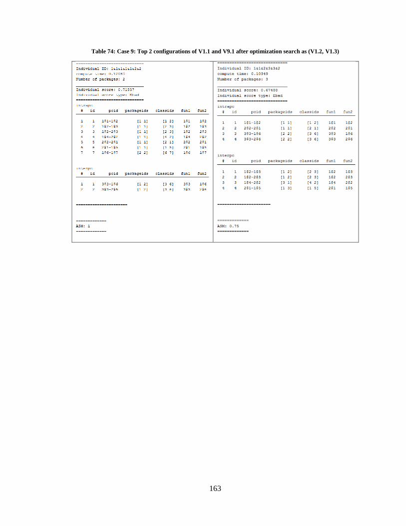
163
Table 74: Case 9: Top 2 configurations of V1.1 and V9.1 after optimization search as (V1.2, V1.3)
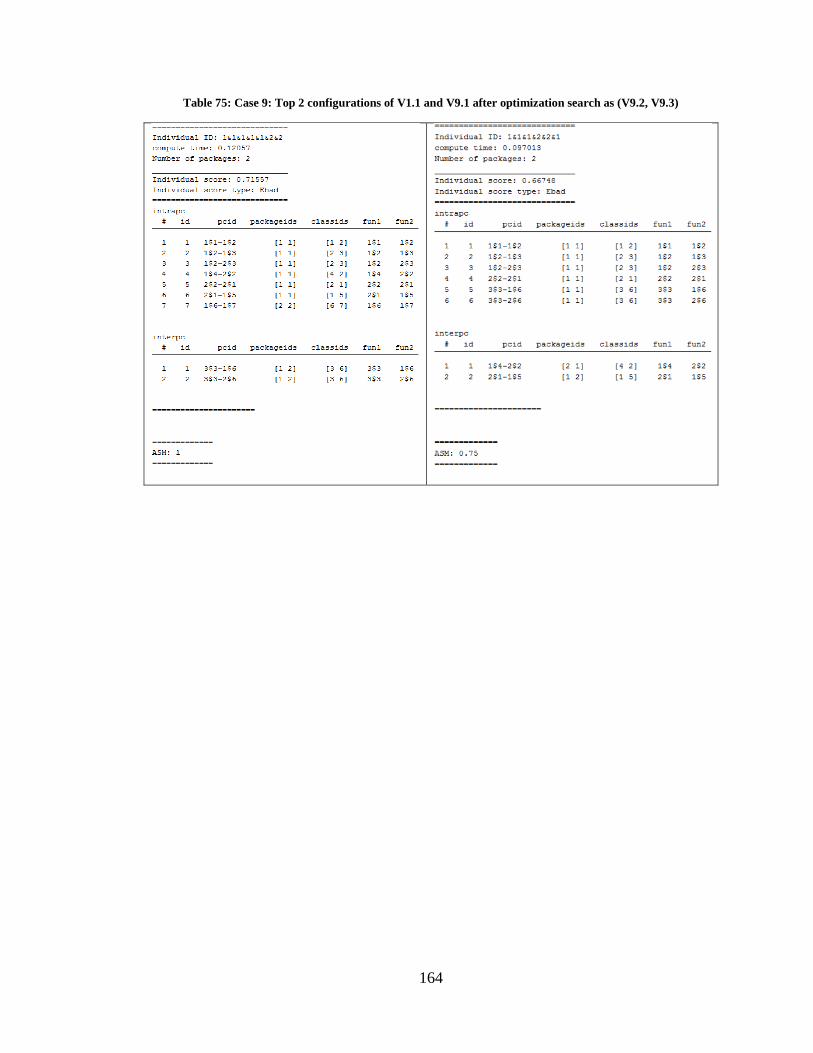
164
Table 75: Case 9: Top 2 configurations of V1.1 and V9.1 after optimization search as (V9.2, V9.3)
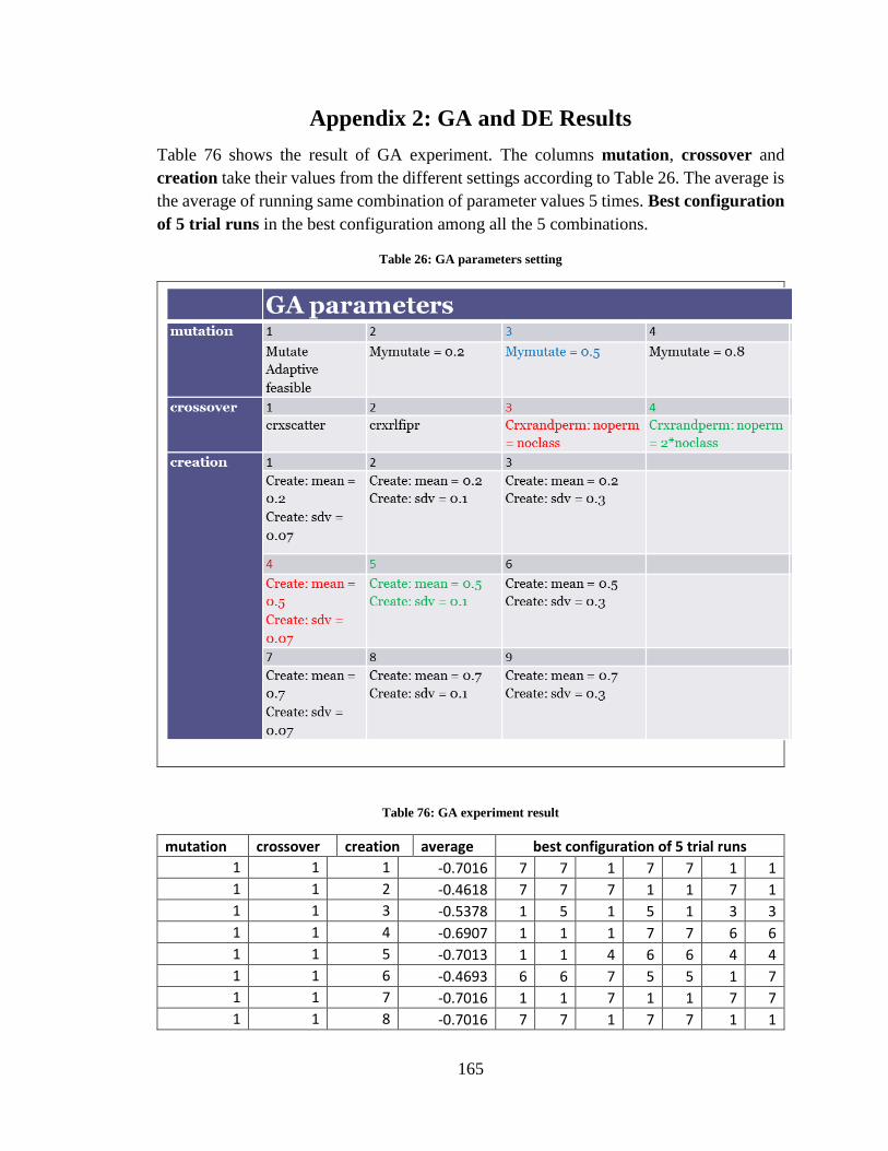
165
Appendix 2: GA and DE Results
Table 76 shows the result of GA experiment. The columns mutation, crossover and
creation take their values from the different settings according to Table 26. The average is
the average of running same combination of parameter values 5 times. Best configuration
of 5 trial runs in the best configuration among all the 5 combinations.
Table 26: GA parameters setting
Table 76: GA experiment result
mutation crossover creation average best configuration of 5 trial runs
1 1 1 -0.7016 7 7 1 7 7 1 1
1 1 2 -0.4618 7 7 7 1 1 7 1
1 1 3 -0.5378 1 5 1 5 1 3 3
1 1 4 -0.6907 1 1 1 7 7 6 6
1 1 5 -0.7013 1 1 4 6 6 4 4
1 1 6 -0.4693 6 6 7 5 5 1 7
1 1 7 -0.7016 1 1 7 1 1 7 7
1 1 8 -0.7016 7 7 1 7 7 1 1
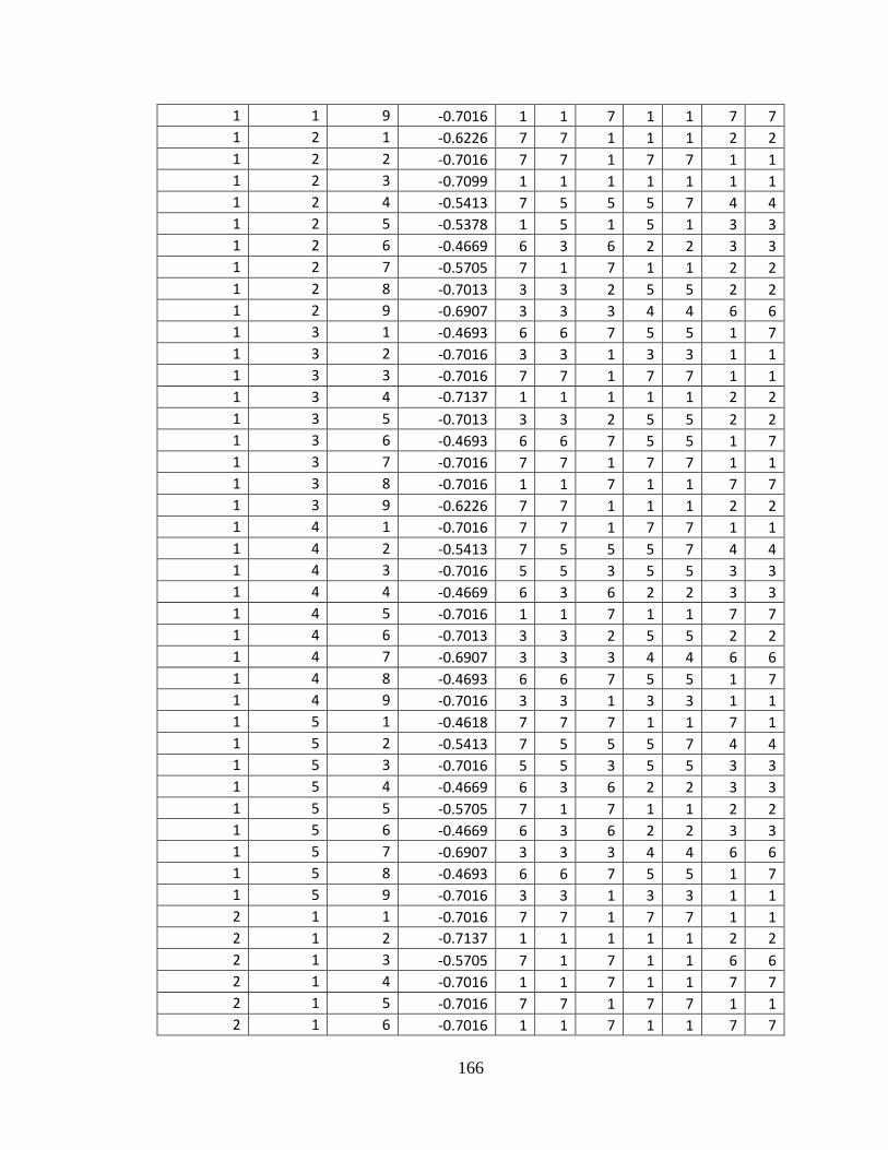
166
1 1 9 -0.7016 1 1 7 1 1 7 7
1 2 1 -0.6226 7 7 1 1 1 2 2
1 2 2 -0.7016 7 7 1 7 7 1 1
1 2 3 -0.7099 1 1 1 1 1 1 1
1 2 4 -0.5413 7 5 5 5 7 4 4
1 2 5 -0.5378 1 5 1 5 1 3 3
1 2 6 -0.4669 6 3 6 2 2 3 3
1 2 7 -0.5705 7 1 7 1 1 2 2
1 2 8 -0.7013 3 3 2 5 5 2 2
1 2 9 -0.6907 3 3 3 4 4 6 6
1 3 1 -0.4693 6 6 7 5 5 1 7
1 3 2 -0.7016 3 3 1 3 3 1 1
1 3 3 -0.7016 7 7 1 7 7 1 1
1 3 4 -0.7137 1 1 1 1 1 2 2
1 3 5 -0.7013 3 3 2 5 5 2 2
1 3 6 -0.4693 6 6 7 5 5 1 7
1 3 7 -0.7016 7 7 1 7 7 1 1
1 3 8 -0.7016 1 1 7 1 1 7 7
1 3 9 -0.6226 7 7 1 1 1 2 2
1 4 1 -0.7016 7 7 1 7 7 1 1
1 4 2 -0.5413 7 5 5 5 7 4 4
1 4 3 -0.7016 5 5 3 5 5 3 3
1 4 4 -0.4669 6 3 6 2 2 3 3
1 4 5 -0.7016 1 1 7 1 1 7 7
1 4 6 -0.7013 3 3 2 5 5 2 2
1 4 7 -0.6907 3 3 3 4 4 6 6
1 4 8 -0.4693 6 6 7 5 5 1 7
1 4 9 -0.7016 3 3 1 3 3 1 1
1 5 1 -0.4618 7 7 7 1 1 7 1
1 5 2 -0.5413 7 5 5 5 7 4 4
1 5 3 -0.7016 5 5 3 5 5 3 3
1 5 4 -0.4669 6 3 6 2 2 3 3
1 5 5 -0.5705 7 1 7 1 1 2 2
1 5 6 -0.4669 6 3 6 2 2 3 3
1 5 7 -0.6907 3 3 3 4 4 6 6
1 5 8 -0.4693 6 6 7 5 5 1 7
1 5 9 -0.7016 3 3 1 3 3 1 1
2 1 1 -0.7016 7 7 1 7 7 1 1
2 1 2 -0.7137 1 1 1 1 1 2 2
2 1 3 -0.5705 7 1 7 1 1 6 6
2 1 4 -0.7016 1 1 7 1 1 7 7
2 1 5 -0.7016 7 7 1 7 7 1 1
2 1 6 -0.7016 1 1 7 1 1 7 7
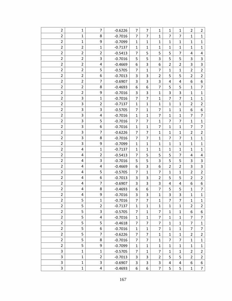
167
2 1 7 -0.6226 7 7 1 1 1 2 2
2 1 8 -0.7016 7 7 1 7 7 1 1
2 1 9 -0.7099 1 1 1 1 1 1 1
2 2 1 -0.7137 1 1 1 1 1 1 1
2 2 2 -0.5413 7 5 5 5 7 4 4
2 2 3 -0.7016 5 5 3 5 5 3 3
2 2 4 -0.4669 6 3 6 2 2 3 3
2 2 5 -0.5705 7 1 7 1 1 2 2
2 2 6 -0.7013 3 3 2 5 5 2 2
2 2 7 -0.6907 3 3 3 4 4 6 6
2 2 8 -0.4693 6 6 7 5 5 1 7
2 2 9 -0.7016 3 3 1 3 3 1 1
2 3 1 -0.7016 7 7 1 7 7 1 1
2 3 2 -0.7137 1 1 1 1 1 2 2
2 3 3 -0.5705 7 1 7 1 1 6 6
2 3 4 -0.7016 1 1 7 1 1 7 7
2 3 5 -0.7016 7 7 1 7 7 1 1
2 3 6 -0.7016 1 1 7 1 1 7 7
2 3 7 -0.6226 7 7 1 1 1 2 2
2 3 8 -0.7016 7 7 1 7 7 1 1
2 3 9 -0.7099 1 1 1 1 1 1 1
2 4 1 -0.7137 1 1 1 1 1 1 1
2 4 2 -0.5413 7 5 5 5 7 4 4
2 4 3 -0.7016 5 5 3 5 5 3 3
2 4 4 -0.4669 6 3 6 2 2 3 3
2 4 5 -0.5705 7 1 7 1 1 2 2
2 4 6 -0.7013 3 3 2 5 5 2 2
2 4 7 -0.6907 3 3 3 4 4 6 6
2 4 8 -0.4693 6 6 7 5 5 1 7
2 4 9 -0.7016 3 3 1 3 3 1 1
2 5 1 -0.7016 7 7 1 7 7 1 1
2 5 2 -0.7137 1 1 1 1 1 2 2
2 5 3 -0.5705 7 1 7 1 1 6 6
2 5 4 -0.7016 1 1 7 1 1 7 7
2 5 5 -0.4618 7 7 7 1 1 7 1
2 5 6 -0.7016 1 1 7 1 1 7 7
2 5 7 -0.6226 7 7 1 1 1 2 2
2 5 8 -0.7016 7 7 1 7 7 1 1
2 5 9 -0.7099 1 1 1 1 1 1 1
3 1 1 -0.5705 7 1 7 1 1 2 2
3 1 2 -0.7013 3 3 2 5 5 2 2
3 1 3 -0.6907 3 3 3 4 4 6 6
3 1 4 -0.4693 6 6 7 5 5 1 7
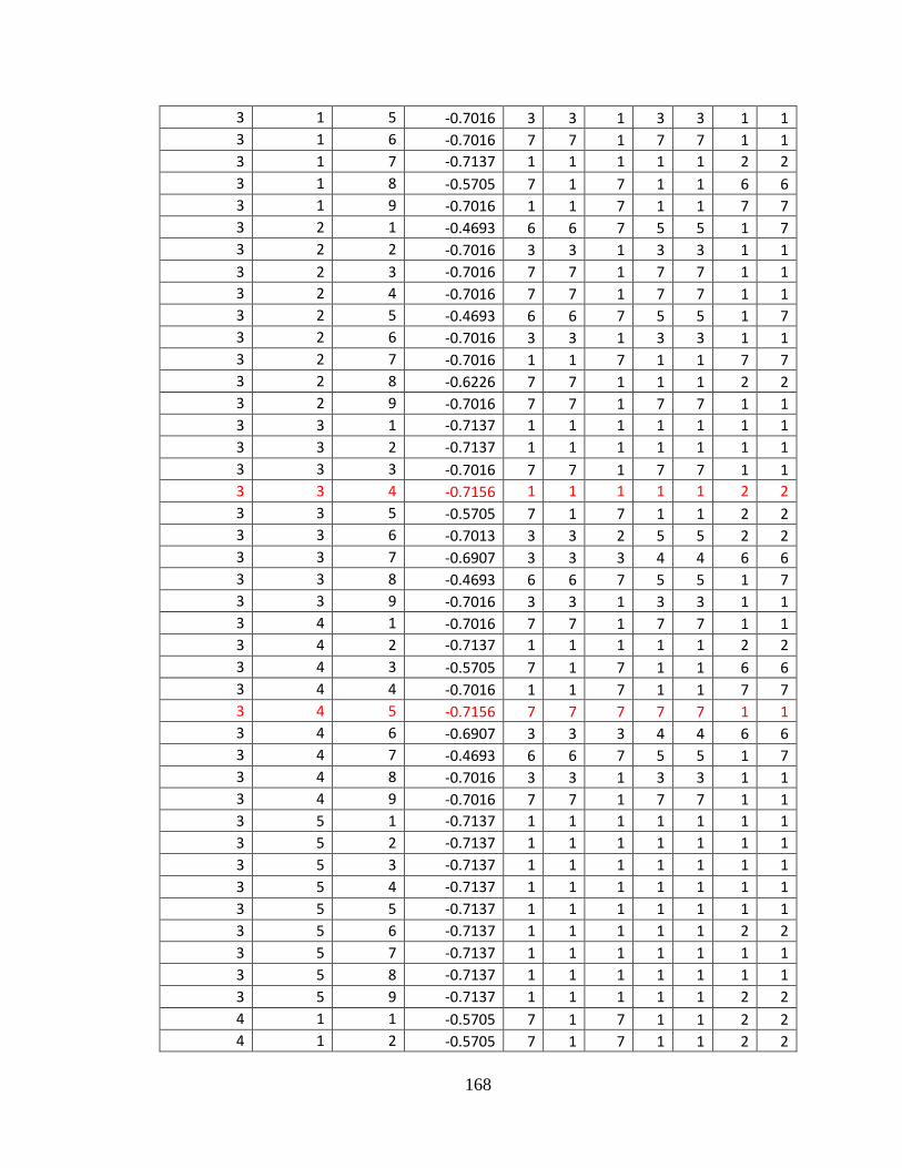
168
3 1 5 -0.7016 3 3 1 3 3 1 1
3 1 6 -0.7016 7 7 1 7 7 1 1
3 1 7 -0.7137 1 1 1 1 1 2 2
3 1 8 -0.5705 7 1 7 1 1 6 6
3 1 9 -0.7016 1 1 7 1 1 7 7
3 2 1 -0.4693 6 6 7 5 5 1 7
3 2 2 -0.7016 3 3 1 3 3 1 1
3 2 3 -0.7016 7 7 1 7 7 1 1
3 2 4 -0.7016 7 7 1 7 7 1 1
3 2 5 -0.4693 6 6 7 5 5 1 7
3 2 6 -0.7016 3 3 1 3 3 1 1
3 2 7 -0.7016 1 1 7 1 1 7 7
3 2 8 -0.6226 7 7 1 1 1 2 2
3 2 9 -0.7016 7 7 1 7 7 1 1
3 3 1 -0.7137 1 1 1 1 1 1 1
3 3 2 -0.7137 1 1 1 1 1 1 1
3 3 3 -0.7016 7 7 1 7 7 1 1
3 3 4 -0.7156 1 1 1 1 1 2 2
3 3 5 -0.5705 7 1 7 1 1 2 2
3 3 6 -0.7013 3 3 2 5 5 2 2
3 3 7 -0.6907 3 3 3 4 4 6 6
3 3 8 -0.4693 6 6 7 5 5 1 7
3 3 9 -0.7016 3 3 1 3 3 1 1
3 4 1 -0.7016 7 7 1 7 7 1 1
3 4 2 -0.7137 1 1 1 1 1 2 2
3 4 3 -0.5705 7 1 7 1 1 6 6
3 4 4 -0.7016 1 1 7 1 1 7 7
3 4 5 -0.7156 7 7 7 7 7 1 1
3 4 6 -0.6907 3 3 3 4 4 6 6
3 4 7 -0.4693 6 6 7 5 5 1 7
3 4 8 -0.7016 3 3 1 3 3 1 1
3 4 9 -0.7016 7 7 1 7 7 1 1
3 5 1 -0.7137 1 1 1 1 1 1 1
3 5 2 -0.7137 1 1 1 1 1 1 1
3 5 3 -0.7137 1 1 1 1 1 1 1
3 5 4 -0.7137 1 1 1 1 1 1 1
3 5 5 -0.7137 1 1 1 1 1 1 1
3 5 6 -0.7137 1 1 1 1 1 2 2
3 5 7 -0.7137 1 1 1 1 1 1 1
3 5 8 -0.7137 1 1 1 1 1 1 1
3 5 9 -0.7137 1 1 1 1 1 2 2
4 1 1 -0.5705 7 1 7 1 1 2 2
4 1 2 -0.5705 7 1 7 1 1 2 2
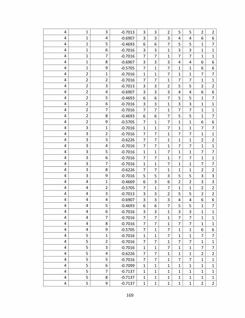
169
4 1 3 -0.7013 3 3 2 5 5 2 2
4 1 4 -0.6907 3 3 3 4 4 6 6
4 1 5 -0.4693 6 6 7 5 5 1 7
4 1 6 -0.7016 3 3 1 3 3 1 1
4 1 7 -0.7016 7 7 1 7 7 1 1
4 1 8 -0.6907 3 3 3 4 4 6 6
4 1 9 -0.5705 7 1 7 1 1 6 6
4 2 1 -0.7016 1 1 7 1 1 7 7
4 2 2 -0.7016 7 7 1 7 7 1 1
4 2 3 -0.7013 3 3 2 5 5 2 2
4 2 4 -0.6907 3 3 3 4 4 6 6
4 2 5 -0.4693 6 6 7 5 5 1 7
4 2 6 -0.7016 3 3 1 3 3 1 1
4 2 7 -0.7016 7 7 1 7 7 1 1
4 2 8 -0.4693 6 6 7 5 5 1 7
4 2 9 -0.5705 7 1 7 1 1 6 6
4 3 1 -0.7016 1 1 7 1 1 7 7
4 3 2 -0.7016 7 7 1 7 7 1 1
4 3 3 -0.6226 7 7 1 1 1 2 2
4 3 4 -0.7016 7 7 1 7 7 1 1
4 3 5 -0.7016 1 1 7 1 1 7 7
4 3 6 -0.7016 7 7 1 7 7 1 1
4 3 7 -0.7016 1 1 7 1 1 7 7
4 3 8 -0.6226 7 7 1 1 1 2 2
4 3 9 -0.7016 5 5 3 5 5 3 3
4 4 1 -0.4669 6 3 6 2 2 3 3
4 4 2 -0.5705 7 1 7 1 1 2 2
4 4 3 -0.7013 3 3 2 5 5 2 2
4 4 4 -0.6907 3 3 3 4 4 6 6
4 4 5 -0.4693 6 6 7 5 5 1 7
4 4 6 -0.7016 3 3 1 3 3 1 1
4 4 7 -0.7016 7 7 1 7 7 1 1
4 4 8 -0.7016 7 7 1 7 7 1 1
4 4 9 -0.5705 7 1 7 1 1 6 6
4 5 1 -0.7016 1 1 7 1 1 7 7
4 5 2 -0.7016 7 7 1 7 7 1 1
4 5 3 -0.7016 1 1 7 1 1 7 7
4 5 4 -0.6226 7 7 1 1 1 2 2
4 5 5 -0.7016 7 7 1 7 7 1 1
4 5 6 -0.7099 1 1 1 1 1 1 1
4 5 7 -0.7137 1 1 1 1 1 1 1
4 5 8 -0.7137 1 1 1 1 1 1 1
4 5 9 -0.7137 1 1 1 1 1 2 2
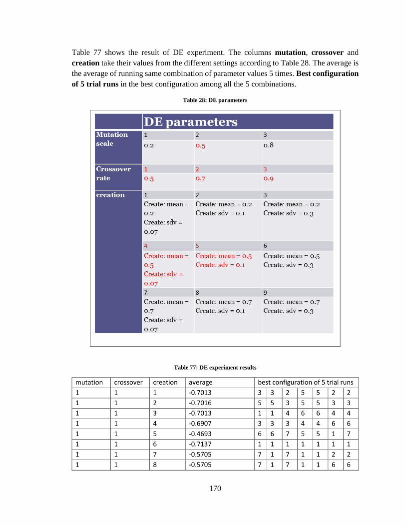
170
Table 77 shows the result of DE experiment. The columns mutation, crossover and
creation take their values from the different settings according to Table 28. The average is
the average of running same combination of parameter values 5 times. Best configuration
of 5 trial runs in the best configuration among all the 5 combinations.
Table 28: DE parameters
Table 77: DE experiment results
mutation crossover creation average best configuration of 5 trial runs
1 1 1 -0.7013 3 3 2 5 5 2 2
1 1 2 -0.7016 5 5 3 5 5 3 3
1 1 3 -0.7013 1 1 4 6 6 4 4
1 1 4 -0.6907 3 3 3 4 4 6 6
1 1 5 -0.4693 6 6 7 5 5 1 7
1 1 6 -0.7137 1 1 1 1 1 1 1
1 1 7 -0.5705 7 1 7 1 1 2 2
1 1 8 -0.5705 7 1 7 1 1 6 6
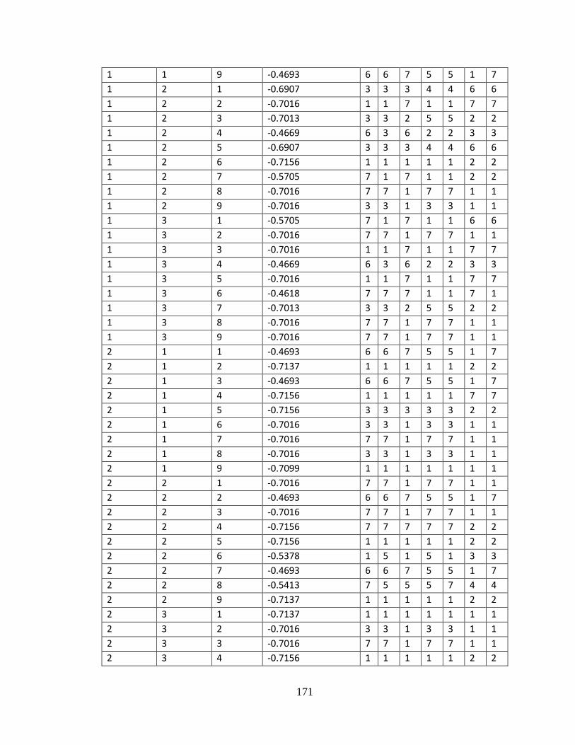
171
1 1 9 -0.4693 6 6 7 5 5 1 7
1 2 1 -0.6907 3 3 3 4 4 6 6
1 2 2 -0.7016 1 1 7 1 1 7 7
1 2 3 -0.7013 3 3 2 5 5 2 2
1 2 4 -0.4669 6 3 6 2 2 3 3
1 2 5 -0.6907 3 3 3 4 4 6 6
1 2 6 -0.7156 1 1 1 1 1 2 2
1 2 7 -0.5705 7 1 7 1 1 2 2
1 2 8 -0.7016 7 7 1 7 7 1 1
1 2 9 -0.7016 3 3 1 3 3 1 1
1 3 1 -0.5705 7 1 7 1 1 6 6
1 3 2 -0.7016 7 7 1 7 7 1 1
1 3 3 -0.7016 1 1 7 1 1 7 7
1 3 4 -0.4669 6 3 6 2 2 3 3
1 3 5 -0.7016 1 1 7 1 1 7 7
1 3 6 -0.4618 7 7 7 1 1 7 1
1 3 7 -0.7013 3 3 2 5 5 2 2
1 3 8 -0.7016 7 7 1 7 7 1 1
1 3 9 -0.7016 7 7 1 7 7 1 1
2 1 1 -0.4693 6 6 7 5 5 1 7
2 1 2 -0.7137 1 1 1 1 1 2 2
2 1 3 -0.4693 6 6 7 5 5 1 7
2 1 4 -0.7156 1 1 1 1 1 7 7
2 1 5 -0.7156 3 3 3 3 3 2 2
2 1 6 -0.7016 3 3 1 3 3 1 1
2 1 7 -0.7016 7 7 1 7 7 1 1
2 1 8 -0.7016 3 3 1 3 3 1 1
2 1 9 -0.7099 1 1 1 1 1 1 1
2 2 1 -0.7016 7 7 1 7 7 1 1
2 2 2 -0.4693 6 6 7 5 5 1 7
2 2 3 -0.7016 7 7 1 7 7 1 1
2 2 4 -0.7156 7 7 7 7 7 2 2
2 2 5 -0.7156 1 1 1 1 1 2 2
2 2 6 -0.5378 1 5 1 5 1 3 3
2 2 7 -0.4693 6 6 7 5 5 1 7
2 2 8 -0.5413 7 5 5 5 7 4 4
2 2 9 -0.7137 1 1 1 1 1 2 2
2 3 1 -0.7137 1 1 1 1 1 1 1
2 3 2 -0.7016 3 3 1 3 3 1 1
2 3 3 -0.7016 7 7 1 7 7 1 1
2 3 4 -0.7156 1 1 1 1 1 2 2
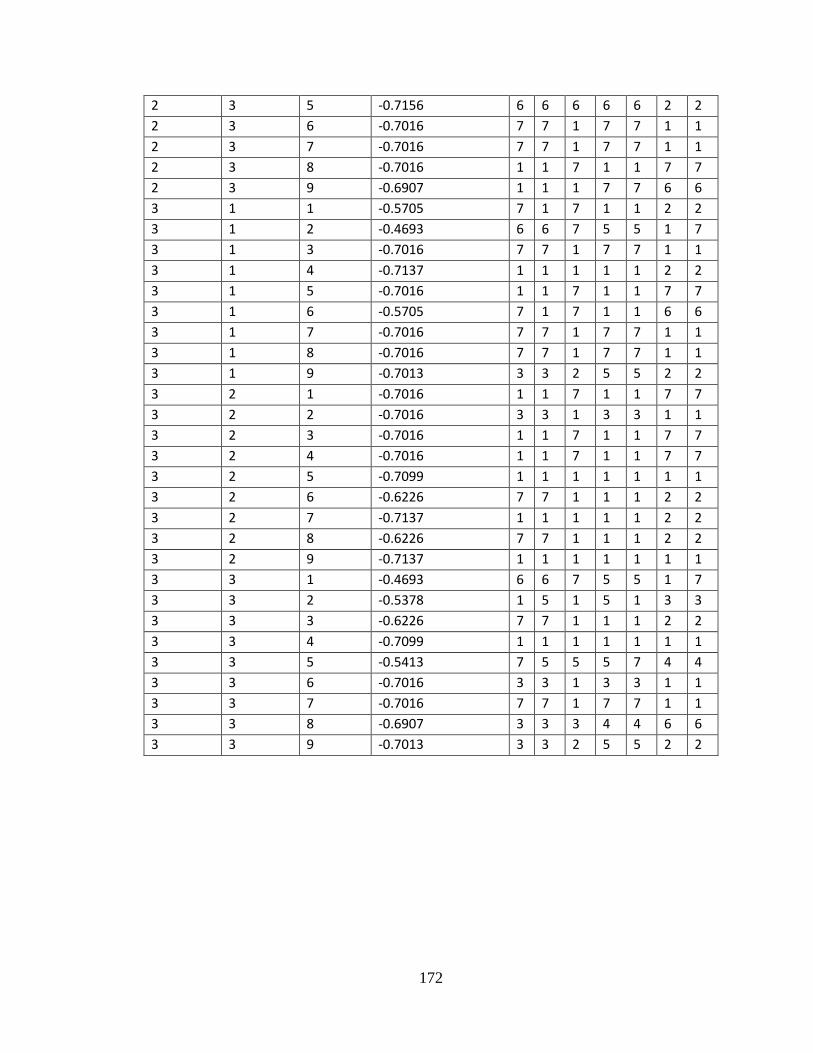
172
2 3 5 -0.7156 6 6 6 6 6 2 2
2 3 6 -0.7016 7 7 1 7 7 1 1
2 3 7 -0.7016 7 7 1 7 7 1 1
2 3 8 -0.7016 1 1 7 1 1 7 7
2 3 9 -0.6907 1 1 1 7 7 6 6
3 1 1 -0.5705 7 1 7 1 1 2 2
3 1 2 -0.4693 6 6 7 5 5 1 7
3 1 3 -0.7016 7 7 1 7 7 1 1
3 1 4 -0.7137 1 1 1 1 1 2 2
3 1 5 -0.7016 1 1 7 1 1 7 7
3 1 6 -0.5705 7 1 7 1 1 6 6
3 1 7 -0.7016 7 7 1 7 7 1 1
3 1 8 -0.7016 7 7 1 7 7 1 1
3 1 9 -0.7013 3 3 2 5 5 2 2
3 2 1 -0.7016 1 1 7 1 1 7 7
3 2 2 -0.7016 3 3 1 3 3 1 1
3 2 3 -0.7016 1 1 7 1 1 7 7
3 2 4 -0.7016 1 1 7 1 1 7 7
3 2 5 -0.7099 1 1 1 1 1 1 1
3 2 6 -0.6226 7 7 1 1 1 2 2
3 2 7 -0.7137 1 1 1 1 1 2 2
3 2 8 -0.6226 7 7 1 1 1 2 2
3 2 9 -0.7137 1 1 1 1 1 1 1
3 3 1 -0.4693 6 6 7 5 5 1 7
3 3 2 -0.5378 1 5 1 5 1 3 3
3 3 3 -0.6226 7 7 1 1 1 2 2
3 3 4 -0.7099 1 1 1 1 1 1 1
3 3 5 -0.5413 7 5 5 5 7 4 4
3 3 6 -0.7016 3 3 1 3 3 1 1
3 3 7 -0.7016 7 7 1 7 7 1 1
3 3 8 -0.6907 3 3 3 4 4 6 6
3 3 9 -0.7013 3 3 2 5 5 2 2

173
Vitae
Name :Aliyu Bagudu
Nationality :Nigeria
Date of Birth :8/13/1988
Email :[email protected]
Address :Bcc house, Bida, Niger state, Nigeria.
Academic Background :B.IT Software Engineering. Multimedia University