image processing point processing filters dithering image compositing image compression point...
Post on 21-Dec-2015
330 views
TRANSCRIPT

Image Processing
Point Processing
Filters
Dithering
Image Compositing
Image Compression
Point Processing
Filters
Dithering
Image Compositing
Image Compression
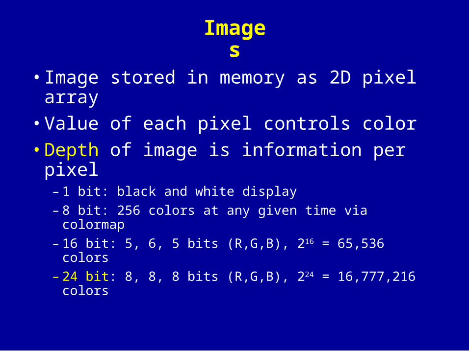
Images
• Image stored in memory as 2D pixel array
• Value of each pixel controls color
• Depth of image is information per pixel– 1 bit: black and white display
– 8 bit: 256 colors at any given time via colormap
– 16 bit: 5, 6, 5 bits (R,G,B), 216 = 65,536 colors
– 24 bit: 8, 8, 8 bits (R,G,B), 224 = 16,777,216 colors
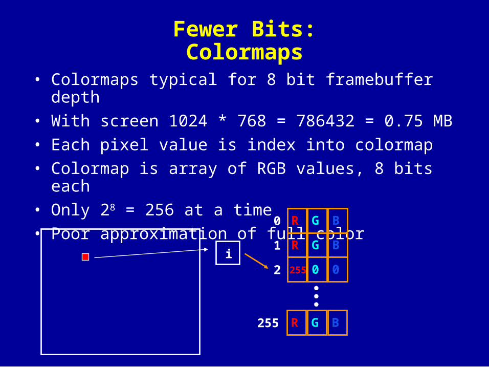
Fewer Bits: Colormaps
• Colormaps typical for 8 bit framebuffer depth
• With screen 1024 * 768 = 786432 = 0.75 MB
• Each pixel value is index into colormap
• Colormap is array of RGB values, 8 bits each
• Only 28 = 256 at a time
• Poor approximation of full color
i
RR GG BB
0
1
2
255
RR GG BB
RR GG BB
255 255 00 00
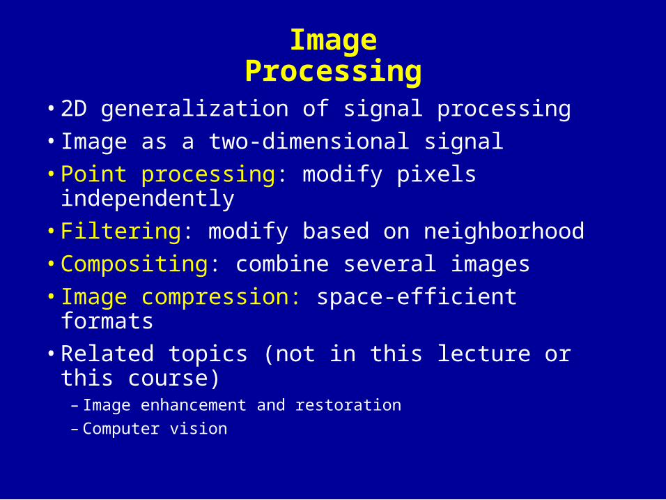
Image Processing
• 2D generalization of signal processing
• Image as a two-dimensional signal
• Point processing: modify pixels independently
• Filtering: modify based on neighborhood
• Compositing: combine several images
• Image compression: space-efficient formats
• Related topics (not in this lecture or this course)– Image enhancement and restoration
– Computer vision
Outline
• Point Processing
• Filters
• Dithering
• Image Compositing
• Image Compression

Point Processing• Input: a[x,y], Output b[x,y] = f(a[x,y])
• f transforms each pixel value separately
• Useful for contrast adjustment
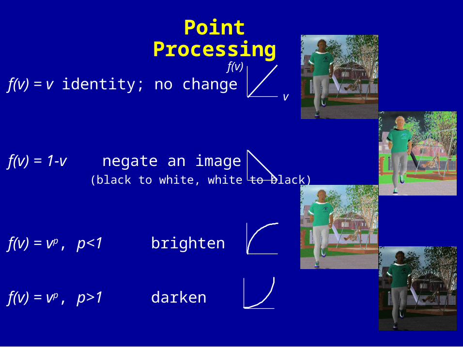
Suppose our picture is grayscale (a.k.a. monochrome).
Let v denote pixel value, suppose it’s in the range [0,1].
f(v) = v identity; no change
f(v) = 1-v negate an image(black to white, white to black)
f(v) = vp, p<1 brighten
f(v) = vp, p>1 darken
v
f(v)
Point Processing
f(v) = v identity; no change
f(v) = 1-v negate an image(black to white, white to black)
f(v) = vp, p<1 brighten
f(v) = vp, p>1 darken
v
f(v)

Gamma correction compensates for different monitors
= 1.0; f(v) = v = 2.5; f(v) = v1/2.5 = v0.4
Monitors have a intensity to voltage response curve which is roughly a 2.5 power function
Send v actually display a pixel which has intensity equal to v2.5
Outline
• Point Processing
• Filters
• Dithering
• Image Compositing
• Image Compression
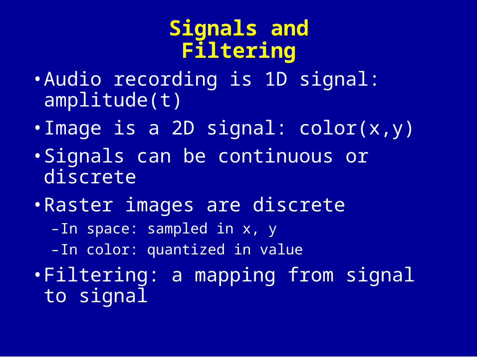
Signals and Filtering
• Audio recording is 1D signal: amplitude(t)
• Image is a 2D signal: color(x,y)
• Signals can be continuous or discrete
• Raster images are discrete–In space: sampled in x, y
–In color: quantized in value
• Filtering: a mapping from signal to signal
Convolution
• Used for filtering, sampling and reconstruction
• Convolution in 1D
Chalkboard
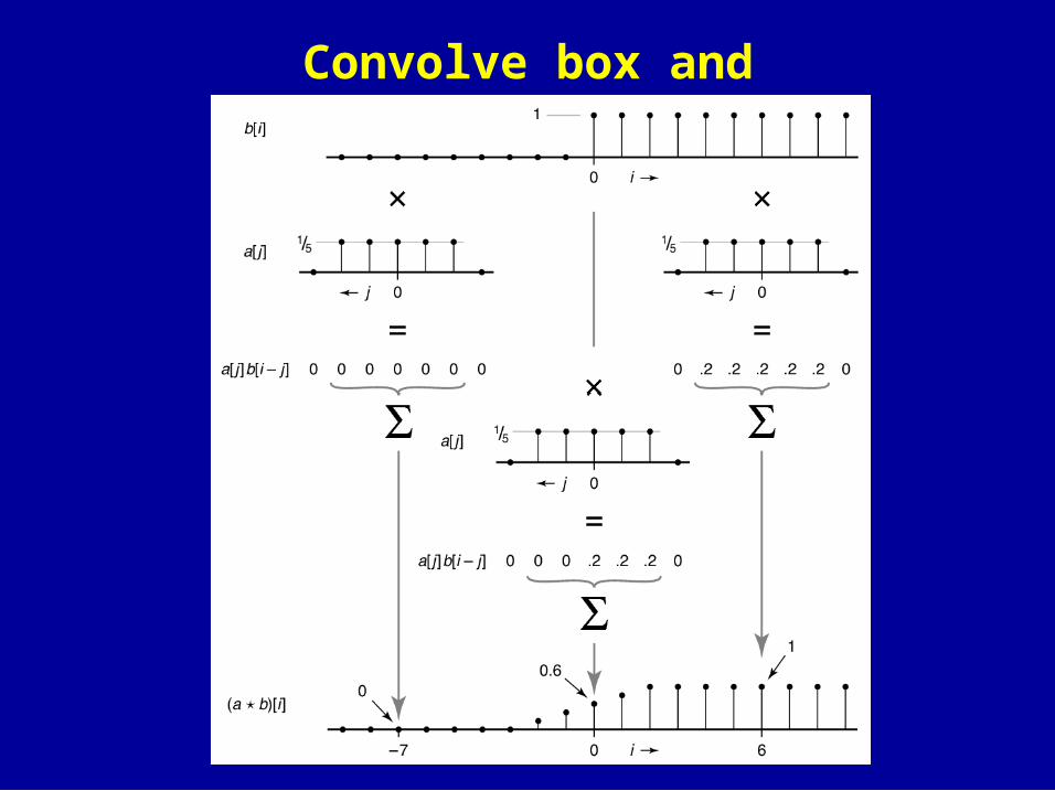
Convolve box and step

Convolution filters
box
tent
gaussian

• Convolution in 1D– a(t) is input signal
– b(s) is output signal
– h(u) is filter
• Convolution in 2D
Convolution filters

Filters with Finite Support
• Filter h(u,v) is 0 except in given region
• Represent h in form of a matrix
• Example: 3 x 3 blurring filter
• As function
• In matrix form
Blurring Filters
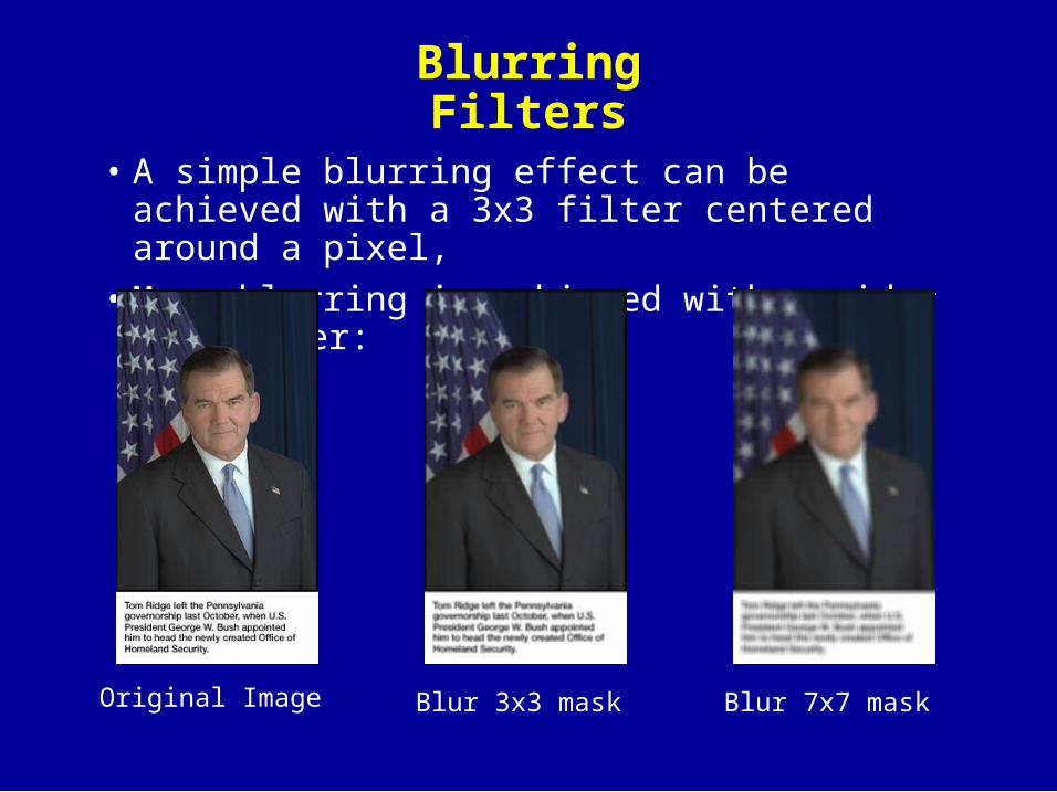
• A simple blurring effect can be achieved with a 3x3 filter centered around a pixel,
• More blurring is achieved with a wider nn filter:
Original Image Blur 3x3 mask Blur 7x7 mask

Image Filtering: Blurring
original, 64x64 pixels 3x3 blur 5x5 blur
Blurring Filters
• Average values of surrounding pixels
• Can be used for anti-aliasing
• What do we do at the edges and corners?
• For noise reduction, use median, not average– Eliminates intensity spikes
– Non-linear filter
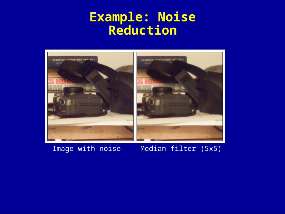
Example: Noise Reduction
Image with noise Median filter (5x5)
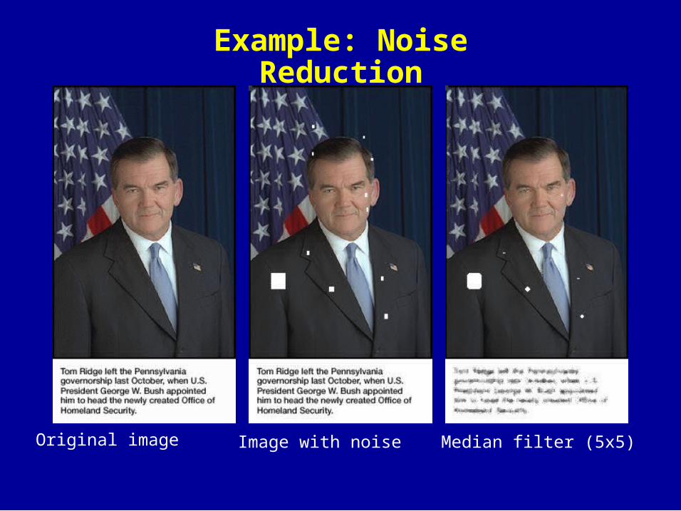
Example: Noise Reduction
Original image Image with noise Median filter (5x5)
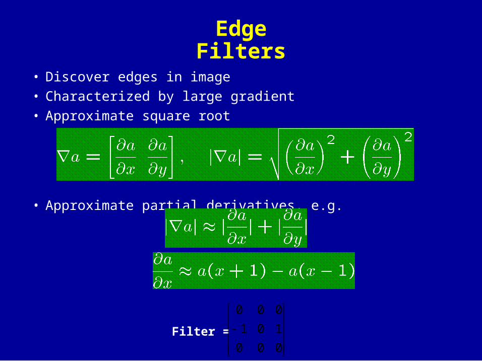
Edge Filters
• Discover edges in image
• Characterized by large gradient
• Approximate square root
• Approximate partial derivatives, e.g.
Filter =
000
101
000
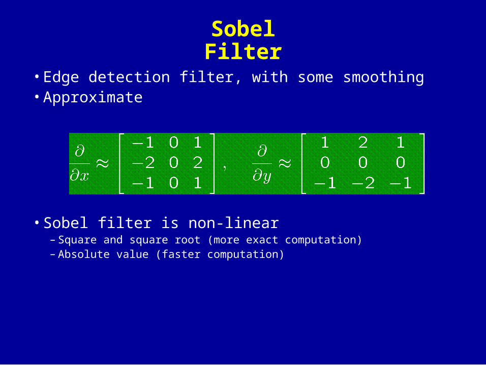
Sobel Filter
• Edge detection filter, with some smoothing• Approximate
• Sobel filter is non-linear– Square and square root (more exact computation)– Absolute value (faster computation)
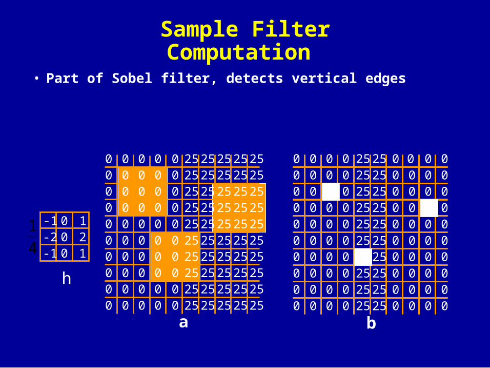
Sample Filter Computation
• Part of Sobel filter, detects vertical edges
-1
-1-2
0
00
1
12
4
125252525252525
252525
25252525252525
252525
25252525252525
252525
25252525252525
252525
25252525252525
252525
0000000
000
0000000
000
0000000
000
0000000
000
0000000
000
a b
25252525252525
252525
0000000
000
0000000
00
0000000
000
0000000
000
25252525252525
252525
0000000
000
0000000
000
0000000
000
0000000
000 0
h
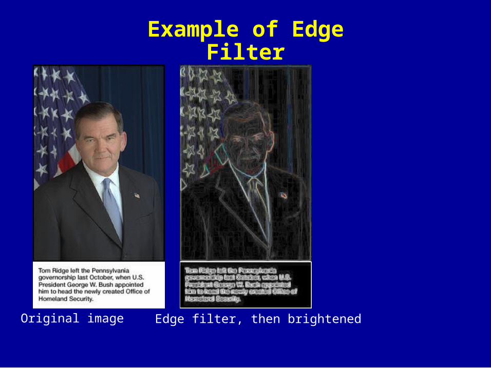
Example of Edge Filter
Original image Edge filter, then brightened
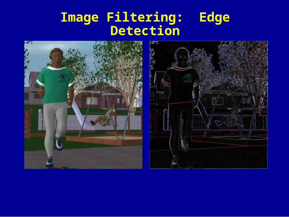
Image Filtering: Edge Detection
Outline
• Display Color Models
• Filters
• Dithering
• Image Compositing
• Image Compression
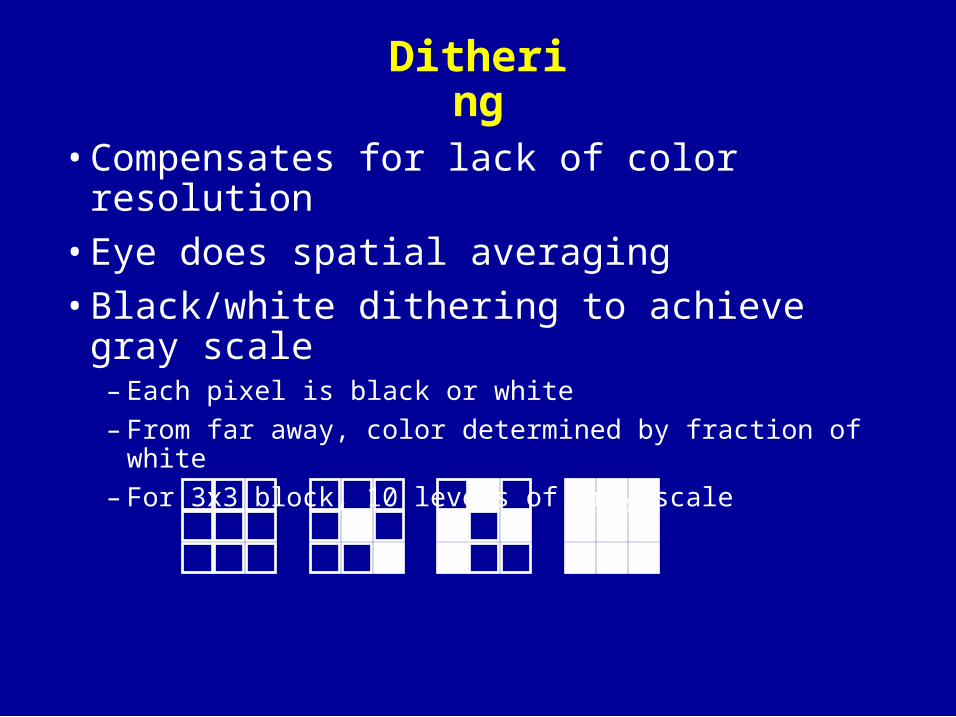
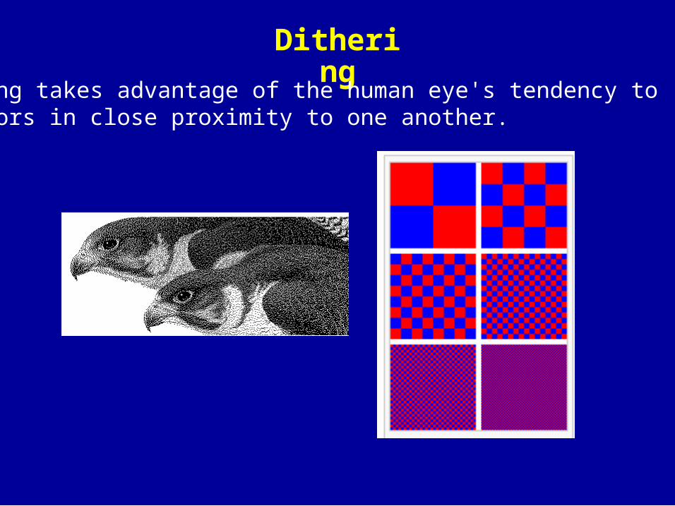
Dithering
• Compensates for lack of color resolution
• Eye does spatial averaging
• Black/white dithering to achieve gray scale– Each pixel is black or white
– From far away, color determined by fraction of white
– For 3x3 block, 10 levels of gray scale
Dithering
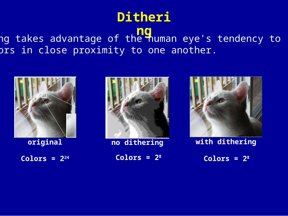
Dithering takes advantage of the human eye's tendency to "mix" two colors in close proximity to one another.
Dithering
Dithering takes advantage of the human eye's tendency to "mix" two colors in close proximity to one another.
original no dithering with dithering
Colors = 224 Colors = 28 Colors = 28
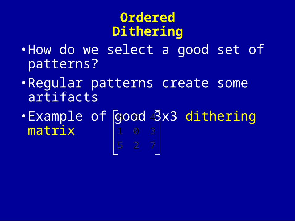
Ordered Dithering
• How do we select a good set of patterns?
• Regular patterns create some artifacts
• Example of good 3x3 dithering matrix
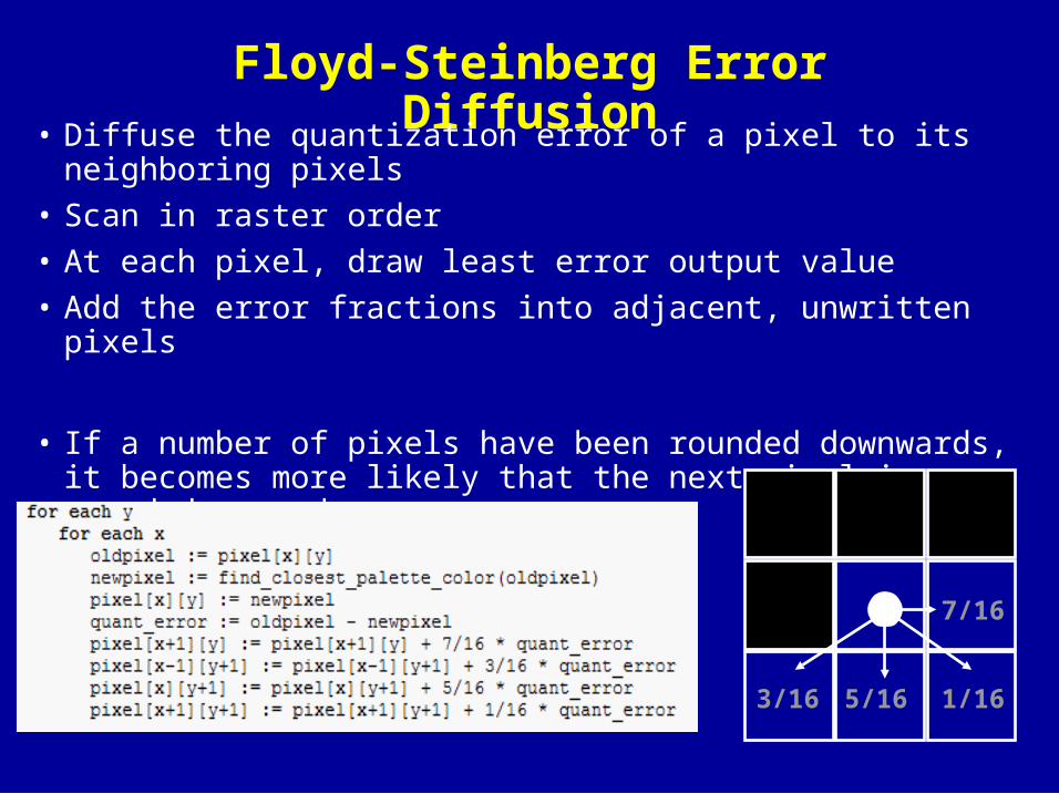
Floyd-Steinberg Error Diffusion• Diffuse the quantization error of a pixel to its neighboring pixels
• Scan in raster order
• At each pixel, draw least error output value
• Add the error fractions into adjacent, unwritten pixels
• If a number of pixels have been rounded downwards, it becomes more likely that the next pixel is rounded upwards
7/16
3/16 5/16 1/16
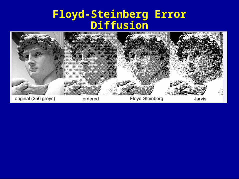
Floyd-Steinberg Error Diffusion
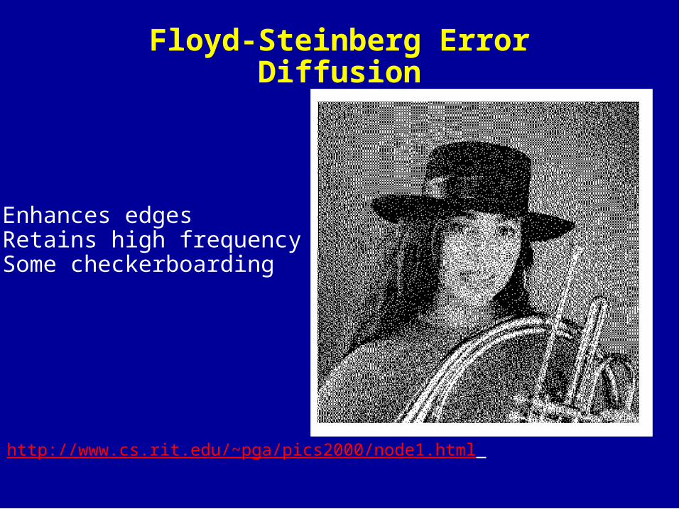
Floyd-Steinberg Error Diffusion
From http://www.cs.rit.edu/~pga/pics2000/node1.html
Enhances edgesRetains high frequencySome checkerboarding

Color Dithering
• Example: 8 bit framebuffer– Set color map by dividing 8 bits into 3,3,2 for RGB
– Blue is deemphasized because we see it less well
• Dither RGB separately– Works well with Floyd-Steinberg
• Generally looks good

Outline
• Display Color Models
• Filters
• Dithering
• Image Compositing
• Image Compression
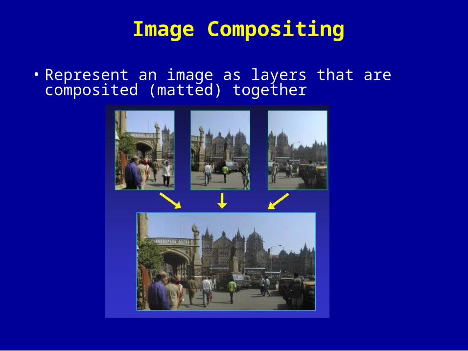
Image Compositing
• Represent an image as layers that are composited (matted) together
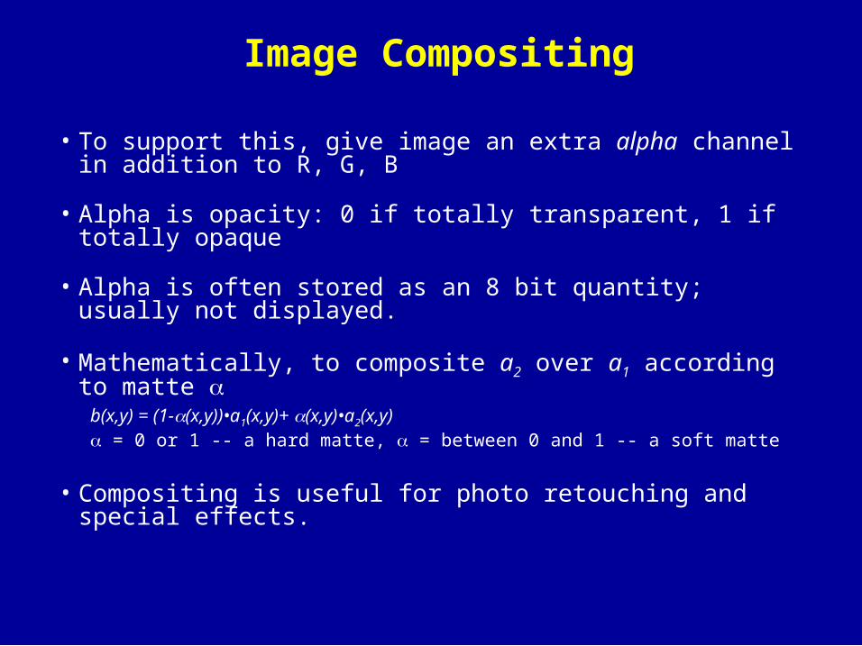
Image Compositing
• To support this, give image an extra alpha channel in addition to R, G, B
• Alpha is opacity: 0 if totally transparent, 1 if totally opaque
• Alpha is often stored as an 8 bit quantity; usually not displayed.
• Mathematically, to composite a2 over a1 according to matte
b(x,y) = (1-(x,y))•a1(x,y)+ (x,y)•a2(x,y) = 0 or 1 -- a hard matte, = between 0 and 1 -- a soft matte
• Compositing is useful for photo retouching and special effects.
Special Effects: Compositing
• Lighting match
• Proper layering
• Contact with the real world
• Realism (perhaps)
• ApplicationsCel animationBlue-screen matting

Roger Rabbit
http://members.tripod.com/~Willy_Wonka/Theatr.jpg
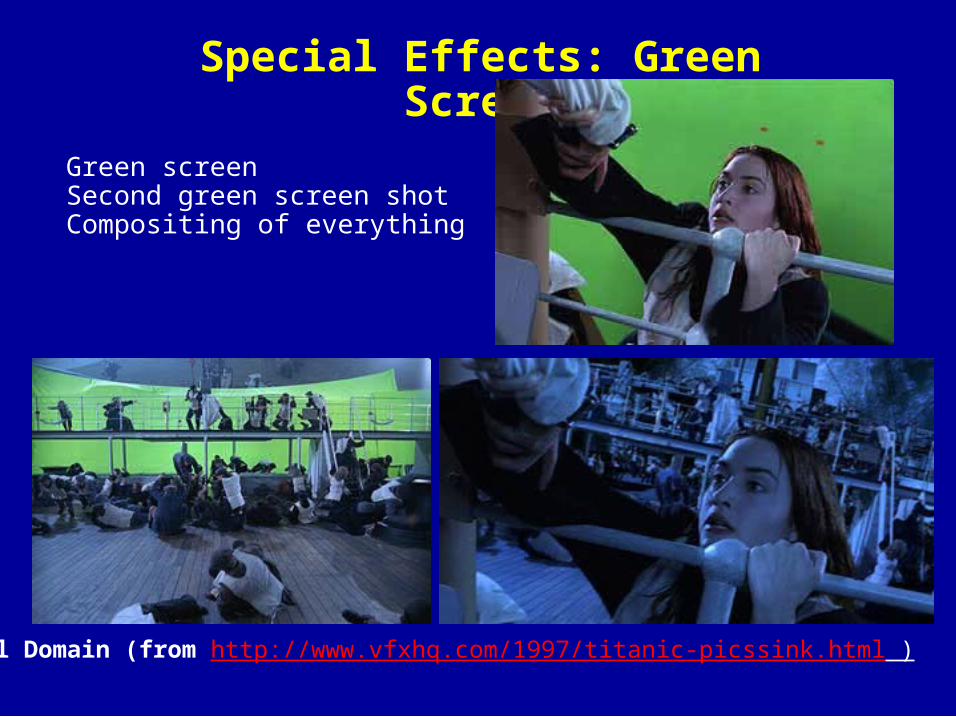
Special Effects: Green Screen
Green screenSecond green screen shotCompositing of everything
Digital Domain (from http://www.vfxhq.com/1997/titanic-picssink.html )
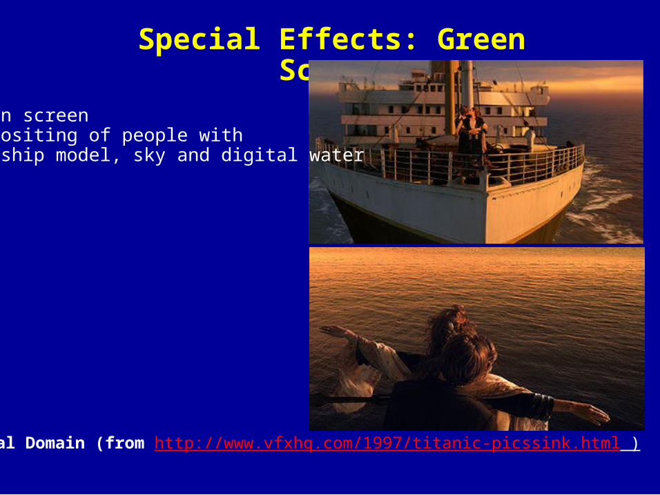
Special Effects: Green Screen
Green screenCompositing of people with ship model, sky and digital water
Digital Domain (from http://www.vfxhq.com/1997/titanic-picssink.html )
Outline
• Display Color Models
• Filters
• Dithering
• Image Compositing
• Image Compression
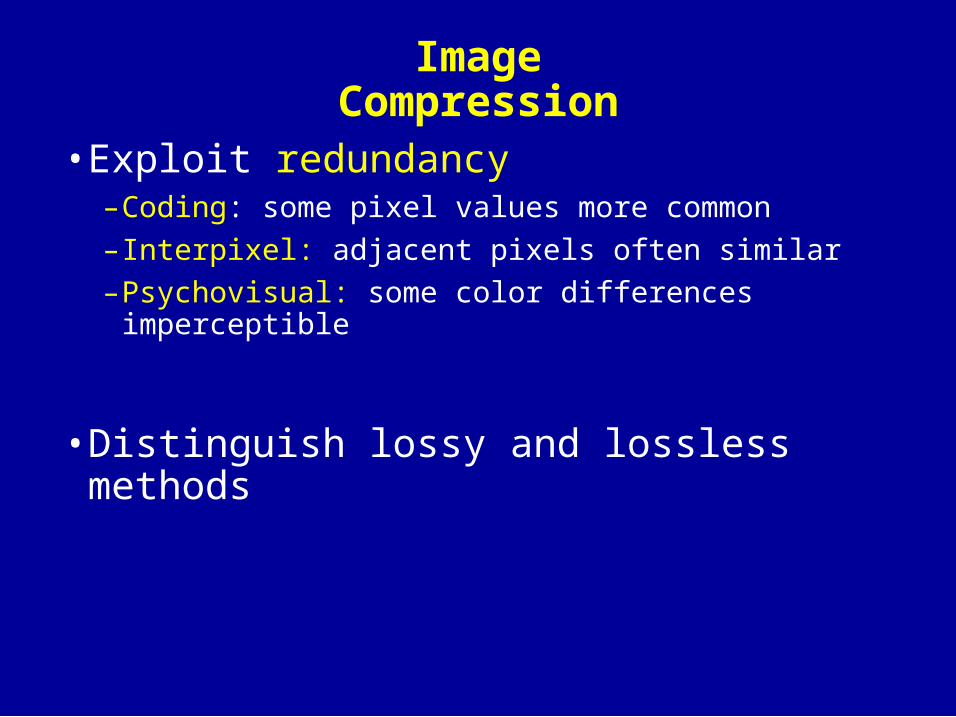
Image Compression
• Exploit redundancy–Coding: some pixel values more common
–Interpixel: adjacent pixels often similar
–Psychovisual: some color differences imperceptible
• Distinguish lossy and lossless methods

Image Sizes
• 1024*1024 at 24 bits uses 3 MB
• Encyclopedia Britannica at 300 pixels/inch and 1 bit/pixes requires 25 gigabytes (25K pages)
• 90 minute movie at 640x480, 24 bits per pixels, 24 frames per second requires 120 gigabytes
• Applications: HDTV, DVD, satellite image transmission, medial image processing, fax, ...
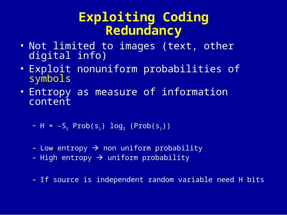
Exploiting Coding Redundancy
• Not limited to images (text, other digital info)• Exploit nonuniform probabilities of symbols• Entropy as measure of information content
– H = -Si Prob(si) log2 (Prob(si))
– Low entropy non uniform probability– High entropy uniform probability
– If source is independent random variable need H bits
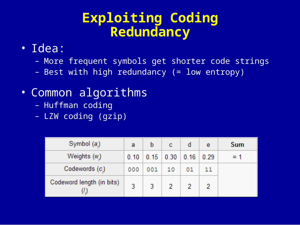
Exploiting Coding Redundancy
• Idea:– More frequent symbols get shorter code strings– Best with high redundancy (= low entropy)
• Common algorithms– Huffman coding– LZW coding (gzip)
Huffman Coding
• Codebook is precomputed and static–Use probability of each symbol to assign code
–Map symbol to code
–Store codebook and code sequence
• Precomputation is expensive
• What is “symbol” for image compression?
lossless
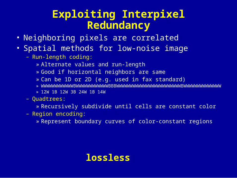
Exploiting Interpixel Redundancy
• Neighboring pixels are correlated• Spatial methods for low-noise image
– Run-length coding:» Alternate values and run-length» Good if horizontal neighbors are same» Can be 1D or 2D (e.g. used in fax standard)» WWWWWWWWWWWWBWWWWWWWWWWWWBBBWWWWWWWWWWWWWWW
WWWWWWWWWBWWWWWWWWWWWWWW » 12W 1B 12W 3B 24W 1B 14W
– Quadtrees:» Recursively subdivide until cells are constant color
– Region encoding:» Represent boundary curves of color-constant regions
lossless
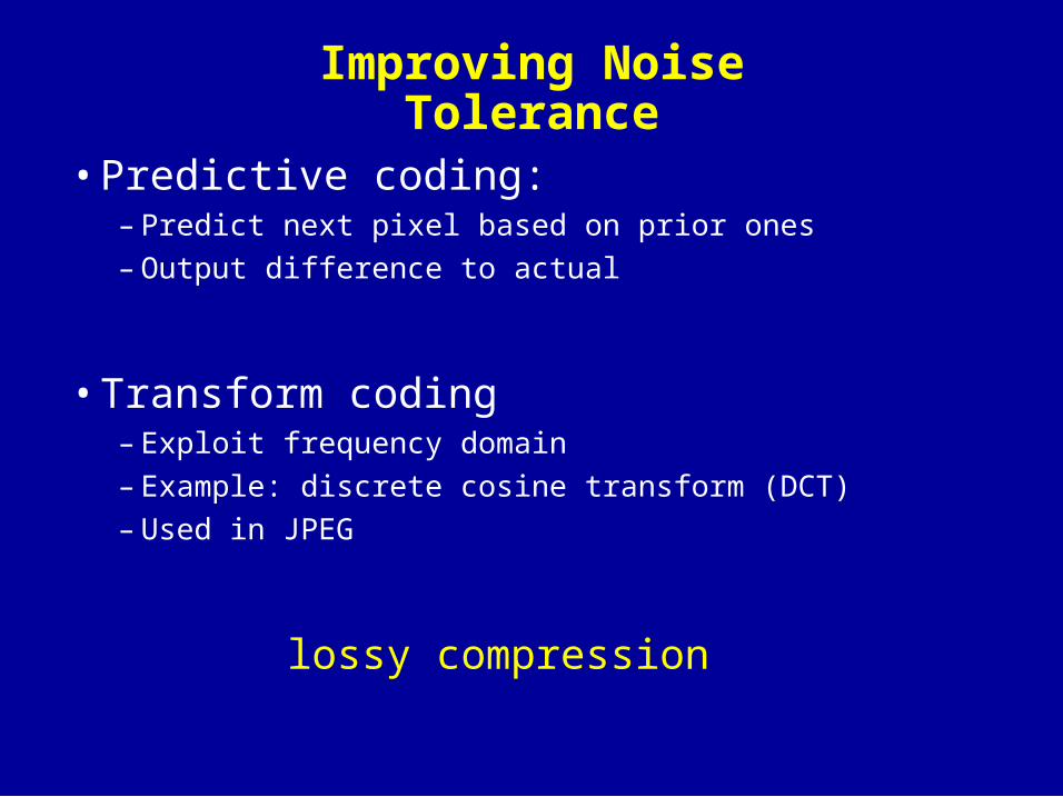
Improving Noise Tolerance
• Predictive coding:– Predict next pixel based on prior ones
– Output difference to actual
• Transform coding– Exploit frequency domain
– Example: discrete cosine transform (DCT)
– Used in JPEG
lossy compression
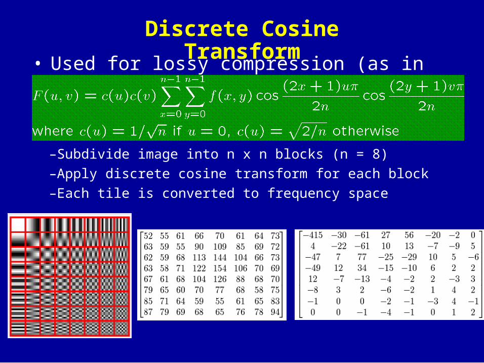
Discrete Cosine Transform• Used for lossy compression (as in JPEG)
–Subdivide image into n x n blocks (n = 8)
–Apply discrete cosine transform for each block
–Each tile is converted to frequency space
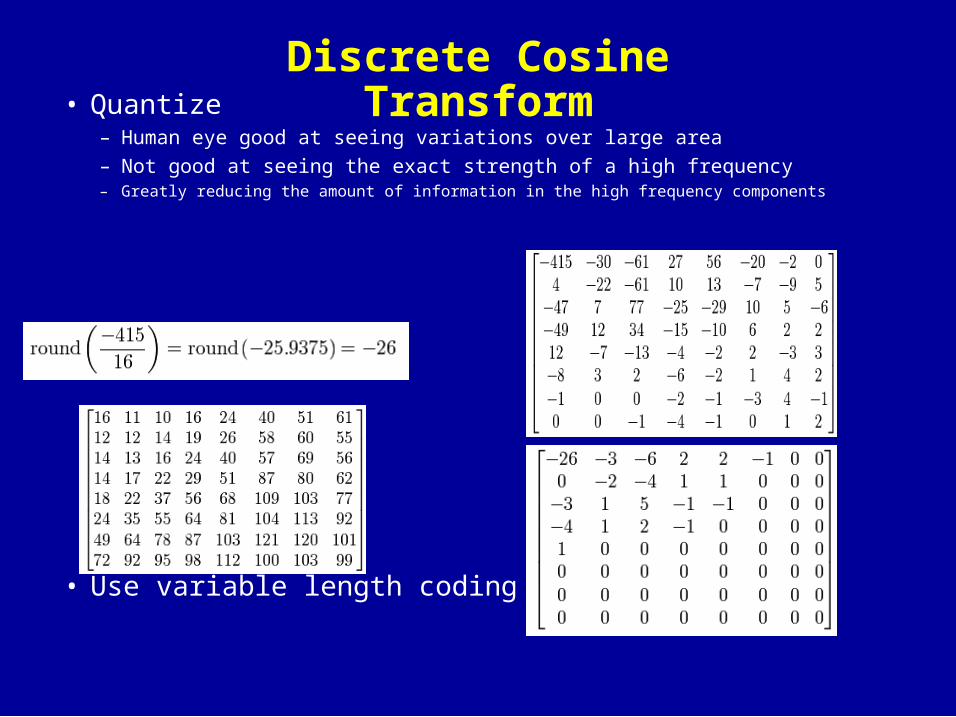
Discrete Cosine Transform• Quantize
– Human eye good at seeing variations over large area
– Not good at seeing the exact strength of a high frequency – Greatly reducing the amount of information in the high frequency components
• Use variable length coding (e.g. Huffman)