gpc and pid controllers applied in a small plant

84 Rev. Tecnol. Fortaleza, v. 29, n. 1, p. 84-90, jun. 2008.

Daniel Thomazini, Maria Virginia Gelfuso, Francisco Teixeira Neto e Éber de Castro Diniz

1 Introduction

Actually there are a lot of control techniques that can be applied in a device, as an electric furnace. The Proportional Derivative Integrative (PID) controller algorithm involves three separate parameters (Liptak, 1995): the Proportional, the Integral and Derivative values. The weighted sum of these three actions is outputted to a control element such as the position of a control valve or power into a heating element. Some applications might require only using one or two modes (by setting undesired control values to zero) to provide the appropriate system control.

A PID controller will be called a PI, PD, P or I controller in the absence of respective control actions. PI controllers are particularly common, since derivative action is very sensitive to measurement noise, and the absence of an integral value prevents the system from ever reaching its target value due to control action.

An interesting approach to unify different ideas of predictive control is Generalized Predictive Control (GPC) according to (Clarke, 1987; Clarke, 1989). It generates a sequence of future control signals within each sampling interval to optimize the control effort of the controlled system. It was done by minimizing a rather complex cost function. Due to the high calculation power required for GPC, real applications in drive systems are very rare. Therefore most papers just present simulation results (Kennel, 2001).

This is the motivation of this paper comparing GPC algorithm (Clarke, 1987) three steps ahead for controlling and PID with parameters adjusted by modified by Ziegler-Nichols Method, and using Extended Least-Squares algorithm (ELS) for identification of the plant.

Daniel ThomaziniUniversidade de Fortaleza, Av. Washington Soares, 1321, [email protected]

Maria Virginia GelfusoUniversidade de Fortaleza, Av. Washington Soares, 1321, [email protected]

Francisco Teixeira NetoUniversidade de Fortaleza, Av. Washington Soares, 1321, [email protected]

Éber de Castro DinizUniversidade de Fortaleza, Av. Washington Soares, 1321, [email protected]

GPC and PID controllers applied in a small plant

ResumoNeste trabalho é proposto o Controle Preditivo Generalizado (GPC) com três passos a frente e outro Proporcional Integrativo Derivativo (PID) para uma planta pequena, utilizando um algoritmo de mínimos quadrados estendido para a identificação da planta. Como resultado obteve-se uma solução de baixo custo e fácil implementação para fornos elétricos, de potência de 2500W. Ambas as aplicações dos controles tiveram uma variação de 0,2% sobre o setpoint em regime permanente, o que pode ser totalmente aceitável, pois uma variação como essa em tratamentos térmicos pode produzir resultados confiáveis. Além disso, esse erro é muito menor quando comparado com um processo manual onde se pode obter erros na ordem de 20 até 30%. O controlador GPC apresentou uma convergência para o setpoint em menor tempo quando comparado com o controlador PID, pois isso ocorreu em 1740 e 8230s, respectivamente.Palavras-chave: GPC. PID. Algoritmo mínimos - quadrados estendido.

AbstractThis work proposes a Generalized Predictive Control (GPC) with three steps ahead for plant controller and Proportional Integrative Derivative (PID) control, using the Extended Least-Squares algorithm for the plant identification. As a result we have a low-cost solution and easy implementation for electrical ovens, in this case, power of 2500W. Both control application had gotten a variation about 0.2% around the setpoint at steady-state, which is acceptable because ±2ºC in thermal treatments can produce reliable results. Also, this error is much better if you compare with manual process that gets an error from 20 to 30%. GPC shows faster convergence to set-point than PID control because it happened in about 1740s, while 8230s for PID control.Keywords: GPC. PID.; Extended least-squares algorithm.

85Rev. Tecnol. Fortaleza, v. 29, n. 1, p. 84-90, jun. 2008.


2 Experimental procedure

An electric oven of 2500W was used in this study. The GPC, PID and ELS algorithms were implemented in a personal computer and interfaced using a microcontroller PIC18F452 with a state solid relay as actuator. All the algorithms were run using Matlab 7.1 with Simulink application. The block diagram of the system is described below.

Figure 1: Block diagram of the system.

On the first iteration, the plant parameters had been already calculated and are allocated in the Matlab, the PID and GPC algorithm calculates the controller parameters three steps ahead. As we have a SISO (Single Input, Single Output) and it is linear, it was first calculated the parameters for power actuator. After signals had sent to the actuator, thermocouple measures the temperature and sends its data to the microcontroller. The microcontroller, having this data and the input parameters calculates the new parameters of the plant using Extended Least-Squares algorithm. So the system has the on-line data for calculating new plant parameters. This system with on-line identification is very useful because changes in the plant parameters are evaluated inside the process, so malfunctioning parts, climate changes are automatically detected, and plant parameters are evaluated on-line, so calculation of controller parameters are well done and more precise.

3 System Identification

The Extended Least-Squares algorithm is a modification in Least-Squares algorithm that envisages reduction in polarized parameters caused by aging of actuators, climate changes or modification in system agents. These methods differ from a different assumption of the noise. While Extended Least-Squares considers a colored noise in its modeling, defining in ARMA (Auto Regressive Moving Average) model, Least-Squares models only a white noise.. So, in our case, modeled plant is described by the following equation:

]1[][]2[

]1[]3[]2[]1[][

2112

11321

−++−+−+−+−+−=

kvdkvdkub

kubkyakyakyaky

(1)

Where y[n] is output of the system, u1[n] is power input and v[k] is white noise. We use the equation 2 to identify the SISO system with regressors vector extended to two inputs (Aguirre, 2002):

(2)

−

−−= ∑∑

=

−

=

N

k

N

k

TMQ kyk

Nkk

N1

1

1)()1(1)1()1(1 ψψψθ



Where the regressors vector are defined as: (3)

Using these mathematical analyses, the identification could be started. The microcontroller sent the required data (the output and input) to the computer, using the serial port. The software received the data and identified the plant parameters, plotting the output of real plant and modeled plant for comparative analyses. Figure 2 shows the real and identified modeling of the plant.

]]1[],[],2[],1[],2[

],1[],3[],2[],1[[)1(

221

1

−−−−−−−−=−

kvkvkukuku

kukykykykψ

Figure 2: Real and online plant identification.

As it can be seen, after 400 seconds, the identified output of modeled plant was close to real one, for the same input. The parameters of the modeled plant, showed in equation 1, calculated with ELS algorithm, were:

a1=1;a2=-1.0125111;a3=0.013296532;b1=0.051108651;b2=0.051050069.

The plant was modeled in third order because the lack of resources (memory) of the microcontroller. We also disconsidered the parameters of colored noise (extended part of identification algorithm) because it would not be useful for GPC controller.

To calculate the parameters of controller we used GPC (Generalized Predictive Control) algorithm, that have been successfully implemented in many industrial applications (Clarke, 1988), “showing performance and certain degree of robustness” (Camacho, 1999).

The basic principle of the GPC resides in the fact that to try to minimize the cost function predicting the future control signals. So, because that this case is a linear model, and a SISO systems as explained previously.

Having this information, we used the CARMA (Controller Auto-Regressive Moving-Average) model for the input. CARMA model has the following equation:

(5)

where: 11 −−=∆ z

The GPC algorithm is described by:

∆+−= −−− /)()()1()()()A(z 11-1 tezCtuzzBty d

0 200 400 600 800 1000150

200

250

300

350

400

450

500

550

IdentifiedReal

Tem

pera

ture

(o C)

Time(s)



(6)

In way that following function minimizes the cost function (or the predictive error). The y(t+j|t) indicates how many steps ahead the algorithm is calculating system output relationed with t variable., N1 and N2 are minimum and maximum horizons of cost function, respectively, and Nu is control horizon. ∆(t) and λ(t) are weighting sequences relationed with time and w(t+j) is at the time t+j. In this case, vector w(t+j) is fixed, since our set point is fixed too, that is, does not vary.

The solution of above function is:

(7)Where K is first line of the matrix, f is free response vector and w is reference vector.G could be solved using the Diophantine equation. But there is an easy way to implement and it is showed below

(Camacho, 1999). As G is a triangular matrix by definition, and diagonals and subdiagonals elements are the same, we use the following equation:

(8)

Where ai and bi are numerator and denominator parameters, respectively. Index j indicates diagonal or subdiagonal number. For example, if j is equal 0, element g0 refers elements of main diagonal, and g1 refers to elements of second di-agonal (or first subdiagonal), and so on. Having these elements we calculate all elements of the G matrix recursively.

Free response could also be calculated by a easier way than using Diophatine equation (Camacho, 1999). Using transfer function of system, we calculate y(t+1), that results in a third equation when we sum y(t) and y(t+1), without white noise(that in our case is only to remove the polarization of the parameters):

]1[][]1[

][]2[]1[][]1[

222112

11321

−++−++−+−+=+

kuckuckub

kubkyakyakyaky

and

]2[]1[]2[

]1[]3[]2[]1[][

222112

11321

−+−+−+−+−+−+−=

kuckuckub

kubkyakyakyaky

which gives:

]2[

]1[)(][)1(]2[

]1[)(][)1(]2[)(

]1[)(][)1(]1[

22

2212112

1211132

211

−+−−+++−+

−−−++−−+−−++=+

kuc

kucckuckub

kubbkubkyaa

kyaakyaky

So, defining f(t+1) = y(t+1) we calculate recursively f(t+n), using same way that we calculate y(t+1), forming free response vector.

4 Modified Ziegler-Nichols method

If an arbitrary point on the Nyquist curve of open-loop system is chosen, the parameters of a PI controller can be calculated in way that this point can be allocated in a suitable position (Aström, 1995). If the chosen point is described by polar coordinates:

[ ]

[ ]∑

∑

=

=

−+∆

++−+=

uN

j

N

NjU

jtuj

jtwtjtyjNNNJ

1

2

221

)1()(

)()|()(),,(2

1

λ

δ

)()( fwKtu −=∆

( ) TT GIGG1−

+ λ



(9)

which must be reallocated, using a controller, to:

(10)

Writing the frequency response of the controller as )( cicerC φ= and using equations (9) and (10):

(11)

The controller should thus be chosen so that: (12)

(13)

For a PI controller this implies: (14) (15)

The point to be moved is usually the ultimate point, which can be determined by relay feedback method (Aström,

)(0 )( ai

aP eriGA φπω +==

)(0 )( bi

beriGB φπι ω +==

)()( cab ica

ib errer φφπφπ +++ =

abc φφφ −=a

cb r

rr =

a

abb

r

rK

)cos( φφ −=

)tan(

1

0 baiT

φφω −=

0 2000 4000 6000 8000 100000

100

200

300

400

500

600

700

GPCPIDTe

mpe

ratu

re(o C)

Time(s)

1995). Has been suggested by Pessen (Pessen, 1954) to move the ultimate point to rb=0.41 and φb=61º.Using this information and the calculated parameters in ELS algorithm, the plant´s output is presented in Figure 3.

Figure 3: Controlled sensor output and set-point.

The steady state error for GPC and PID was, respectively, 0.4% and 1%. Although rise time using PID(650 seconds) was lesser than using GPC (1330 seconds), the first controller drove the system to 23.63% of overshoot, while in GPC the overshoot was only 1,02%. The GPC algorithm stabilized the process in about 1740 seconds, which is a good performance. The PID controller stabilized in 8230 seconds.



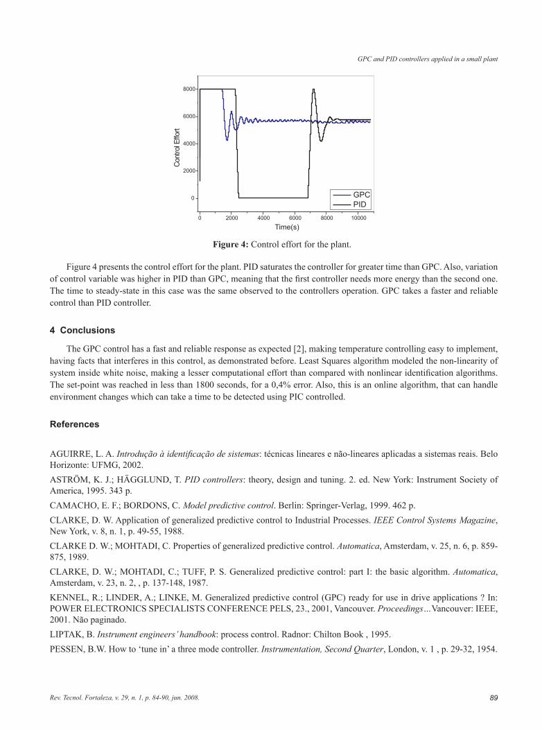
Figure 4: Control effort for the plant.

Figure 4 presents the control effort for the plant. PID saturates the controller for greater time than GPC. Also, variation of control variable was higher in PID than GPC, meaning that the first controller needs more energy than the second one. The time to steady-state in this case was the same observed to the controllers operation. GPC takes a faster and reliable control than PID controller.

4 Conclusions

The GPC control has a fast and reliable response as expected [2], making temperature controlling easy to implement, having facts that interferes in this control, as demonstrated before. Least Squares algorithm modeled the non-linearity of system inside white noise, making a lesser computational effort than compared with nonlinear identification algorithms. The set-point was reached in less than 1800 seconds, for a 0,4% error. Also, this is an online algorithm, that can handle environment changes which can take a time to be detected using PIC controlled.

References

AGUIRRE, L. A. Introdução à identificação de sistemas: técnicas lineares e não-lineares aplicadas a sistemas reais. Belo Horizonte: UFMG, 2002.ASTRÖM, K. J.; HÄGGLUND, T. PID controllers: theory, design and tuning. 2. ed. New York: Instrument Society of America, 1995. 343 p.CAMACHO, E. F.; BORDONS, C. Model predictive control. Berlin: Springer-Verlag, 1999. 462 p.CLARKE, D. W. Application of generalized predictive control to Industrial Processes. IEEE Control Systems Magazine, New York, v. 8, n. 1, p. 49-55, 1988.CLARKE D. W.; MOHTADI, C. Properties of generalized predictive control. Automatica, Amsterdam, v. 25, n. 6, p. 859-875, 1989.CLARKE, D. W.; MOHTADI, C.; TUFF, P. S. Generalized predictive control: part I: the basic algorithm. Automatica, Amsterdam, v. 23, n. 2, , p. 137-148, 1987.KENNEL, R.; LINDER, A.; LINKE, M. Generalized predictive control (GPC) ready for use in drive applications ? In: POWER ELECTRONICS SPECIALISTS CONFERENCE PELS, 23., 2001, Vancouver. Proceedings…Vancouver: IEEE, 2001. Não paginado.LIPTAK, B. Instrument engineers’ handbook: process control. Radnor: Chilton Book , 1995. PESSEN, B.W. How to ‘tune in’ a three mode controller. Instrumentation, Second Quarter, London, v. 1 , p. 29-32, 1954.

0 2000 4000 6000 8000 10000

0

2000

4000

6000

8000

GPCPID

Cont

rolE

ffort

Time(s)



SOBRE OS AUTORES

Daniel ThomaziniEngenheiro de Materiais pela Universidade Federal de São Carlos em 1998, M.Sc. Eng. Materiais pela Universidade Federal do Ceará em 2000, Doutorando em Engenharia Elétrica pela Universidade de São Paulo desde 2005. Atualmente ocupa o cargo de Coordenador de curso de Engenharia de Controle e Automação junto ao Centro de Ciências Tecnológicas da UNIFOR, onde atua em nível de graduação e pós-graduação, tendo orientado alunos de iniciação científica e monografias de especialização. Autor do livro “Sensores Industriais: Fundamento e Aplicações” pela Editora Érica. Atualmente detém quatro depósitos de patentes e artigos publicados em periódicos e congressos nacionais e internacionais.

Maria Virginia GelfusoEngenheira de Materiais pela Universidade Federal de São Carlos em 1991, M.Sc. Eng. Materiais pela Universidade Federal de de São Carlos em 1994, Doutora em Engenharia de Materiais pela Universidade Federal de São Carlos em 1998. Pós-Doutorado pela Universidade Federal de São Carlos em 1999. Atualmente ocupa o cargo de professora Titular junto ao Centro de Ciências Tecnológicas da UNIFOR, onde atua em nível de graduação e pós-graduação, tendo orientado alunos de iniciação científica e monografias de especialização. É coordenadora do Laboratório de Materiais e Instrumentação Eletrônica (LaMatIE), deténdo quatro depósitos de patentes e artigos publicados em periódicos e congressos nacionais e internacionais.

Francisco Teixeira NetoAluno do curso de Engenharia de Controle e Automação na Universidade de Fortaleza desde 2003. Atualmente é bolsista em projetos de pesquisa no LaMatIE. Participou de congressos e eventos na área de automação, tendo publicado um artigo em periódico e dois em eventos internacionais.

Éber de Castro DinizPossui graduação em Engenharia Elétrica pela Universidade Federal do Ceará em 2003. Mestrado em Engenharia Elétrica pela Universidade Federal do Ceará em 2006. Atualmente é professor auxiliar da Universidade de Fortaleza. Tem experiência na área de Engenharia Elétrica, com ênfase em Sistemas de Telecomunicações, atuando principalmente nos seguintes temas: manipulador 2-dof, microcontroladores, controlador de demanda e controladores PID.

gpc and pid controllers applied in a small plant

Documents