Standards

Certification

Education & Training

Publishing

Conferences & Exhibits 1

Effective Use of PID Controllers ISA New Orleans 3-7-2013

2 2

Presenter

– Greg is a retired Senior Fellow from Solutia/Monsanto and an ISA Fellow. Greg was an adjunct professor in the Washington University Saint Louis Chemical Engineering Department 2001-2004. Presently, Greg contracts as a consultant in DeltaV R&D via CDI Process & Industrial and is a part time employee of Experitec and MYNAH. Greg received the ISA “Kermit Fischer Environmental” Award for pH control in 1991, the Control Magazine “Engineer of the Year” Award for the Process Industry in 1994, was inducted into the Control “Process Automation Hall of Fame” in 2001, was honored by InTech Magazine in 2003 as one of the most influential innovators in automation, and received the ISA Life Achievement Award in 2010. Greg is the author of 20 books on process control, his most recent being Advanced Temperature Measurement and Control. Greg has been the monthly “Control Talk” columnist for Control magazine since 2002 and has started a Control Talk Blog. Greg’s expertise is available on the Control Global and Emerson modeling and control web sites: http://community.controlglobal.com/controltalkblog http://modelingandcontrol.com/author/Greg-McMillan/

3

Resources

• (10) Make large setpoint changes that zip past valve dead band and nonlinearities.

• (9) Change the setpoint to operate on the flat part of the titration curve.

• (8) Select the tray with minimum process sensitivity for column temperature control.

• (7) Pick periods when the unit was down.

• (6) Decrease the time span so that just a couple data points are trended.

• (5) Increase the reporting interval so that just a couple data points are trended.

• (4) Use really thick line sizes.

• (3) Add huge signal filters.

• (2) Increase the process variable scale span so it is at least 10x control region

• (1) Increase the historian's data compression so changes are screened out

4

Top Ten Ways to Impress Management with Trends

Contribution of Each PID Mode

• Proportional (P mode) - increase in gain increases P mode contribution – Provides an immediate reaction to magnitude of measurement change to minimize

peak error and integrated error for a disturbance – Too much gain action causes fast oscillations (close to ultimate period) and can make

noise and interactions worse – Provides an immediate reaction to magnitude of setpoint change for P action on Error

to minimize rise time (time to reach setpoint) – Too much gain causes falter in approach to setpoint

• Integral (I mode) - increase in reset time decreases I mode contribution – Provides a ramping reaction to error (SP-PV) to minimize integrated error if stable (since

error is hardly ever exactly zero, integral action is always ramping the controller output) – Too much integral action causes slow oscillations (slower than ultimate period) – Too much integral action causes an overshoot of setpoint (no sense of direction)

• Derivative (D mode) - increase in rate time increases D mode contribution – Provides an immediate reaction to rate of change of measurement change to minimize

peak error and integrated error for a disturbance – Too much rate action causes fast oscillations (faster than ultimate period) and can make

noise and interactions worse – Provides an immediate reaction to rate of change of setpoint change for D action on

Error to minimize rise time (time to reach setpoint) – Too much rate causes fast oscillation in approach to setpoint

Contribution of Each PID Mode

Contribution of Each PID Mode for a Step Change in the Set Point Structure of PID on error (β=1 and γ=1)

kick from filtered derivative mode

∆%CO2 = ∆%CO1

∆%SP

seconds/repeat

∆%CO1

Time (seconds)

Signal (%) step from

proportional mode repeat from

Integral mode

PID structure with proportional, integral, and derivative action on error

Effect of Gain on P-Only Controller Red is 150% of maximum, Green is 100% of maximum, Purple is 50% of maximum of Gain Setting

Effect of Reset Time on PI Controller Red is 150% of maximum, Green is 100% of maximum, Purple is 50% of maximum Reset Time

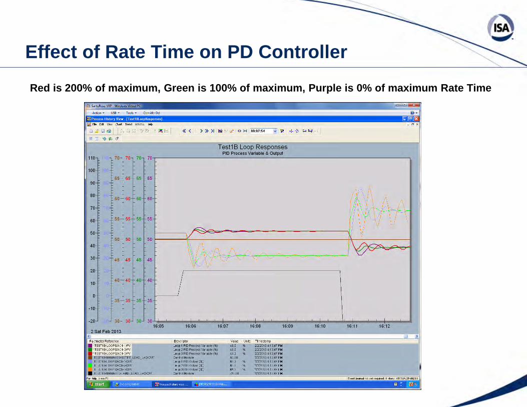
Effect of Rate Time on PD Controller Red is 200% of maximum, Green is 100% of maximum, Purple is 0% of maximum Rate Time

Proportional Mode Basics

Note that many analog controllers used proportional band instead of gain for the proportional mode tuning setting. Proportional band is the % change in the process variable (∆%PV) needed to cause a 100% change in controller output (∆%CO). A 100% proportional band means a 100% ∆%PV would cause a 100 % ∆%CO (a gain of 1). It is critical that users know the units of their controller gain setting and convert accordingly. Gain = 100 % / Proportional Band

• Proportional Mode Advantages • Minimize dead time from stiction and backlash • Minimize rise time • Minimize peak error • Minimize integrated error • Proportional Mode Disadvantages

• Abrupt changes in output upset operators • Abrupt changes in output upset other loops • Amplification of noise

10

Note that many analog controllers used reset settings in repeats per minute instead of reset time for the integral mode tuning setting. Repeats per minute indicate the number of repeats of the proportional mode contribution in a minute. Today’s reset time settings are minutes per repeat or seconds per repeat which gives the time to repeat the proportional mode contribution. Often the “per repeat” term is dropped giving a reset time setting in minutes or seconds. Seconds per repeat = 60 / repeats per minute Integral Mode Advantages • Eliminate offset • Minimize integrated error • Smooth movement of output • Integral Mode Disadvantages • Limit cycles • Overshoot • Runaway of open loop unstable reactors

11

Integral Mode Basics

Nearly all derivative tuning settings are given as a rate time in seconds or minutes. The effective rate time setting must never be greater than the effective reset time setting. The effective settings are for an ISA Standard Form. The advantages and disadvantages of the derivative mode are similar to that of the proportional mode except the relative advantages is less and the relative disadvantages are greater for the derivative mode. Seconds = 60 ∗ minutes • Derivative Mode Advantages

• Minimize dead time from stiction and backlash • Minimize rise time • Minimize peak error • Minimize integrated error • Derivative Mode Disadvantages

• Abrupt changes in output upset operators • Abrupt changes in output upset other loops • Amplification of noise

12

Derivative Mode Basics

SP PV CO

52 48 ?

TC-100 Reactor Temperature

steam valve opens

water valve opens

50%

Should steam or water valve be open ?

Reset Gives Operations What They Want

SP

temperature

time

PV

Open Loop Time Constant (controller in manual)

%CO

Time (seconds)

Signal (%)

0 θo

Dead Time (Time Delay)

τo

Open Loop (process)

Time Constant (Time Lag)

%PV %SP

Controller is in Manual

Open Loop Error Eo (%)

0.63∗Eo

Closed Loop Time Constant (controller in auto)

%CO

Time (seconds)

Signal (%)

0 θo

Dead Time (Time Delay)

τc

Closed Loop Time Constant

(Time Lag) Lambda (λ)

%PV

%SP

Controller is in Automatic

∆%SP

0.63∗∆%SP

• (10) Lots of trials and errors.

• (9) When asked what the controller gain setting is, the answer is given in %.

• (8) When asked what the controller reset time setting is, the answer is in repeats/min.

• (7) The data historian compression setting is 25%.

• (6) There is more recycle than product.

• (5) Valves are wearing out.

• (4) Tempers are wearing thin.

• (3) Operators are placing bets on what loop will cause the next shutdown.

• (2) The output limits are set to keep the valve from moving.

• (1) Preferred mode is manual.

16

Top Ten Signs Loops Need to be Tuned

Conversion of Signals for PID Algorithm

Sensing Element

Control Valve AO PID SCLR

AI

SCLR

SCLR %

% % SUB

%PV SP

%

%CO OUT (e.u.)

Process Equipment

Smart Transmitter PV - Primary Variable

SV - Second Variable* TV - Third Variable* FV - Fourth Variable*

PV (e.u.)

PID

DCS

MV (e.u.)

The scaler block (SCLR) that convert between engineering units of application and % of scale used in PID algorithm is embedded hidden part of the Proportional-Integral-Derivative block (PID)

Final Control Element

Measurement

* - additional HART variables

PV (e.u.)

To compute controller tuning settings, the process variable and controller output must be converted to % of scale and time units of dead times and time constants

must be same as time units of reset time and rate time settings!

18

Series Form

Σ

∗

%SP

β

∆ proportional

integral

derivative

∗

Gain

∗

∗ ∗

∗

Inverse Reset Time

∗

Rate Time

∆

∆

γ

%CO

filter

filter

%PV filter

Filter Time = α ∗ Rate Time

Σ

Switch position for no derivative action

All signals are % of scale in PID algorithm but inputs and outputs are in engineering units

Form in analog controllers and early DCS – available as a choice in most modern DCS

Parallel Form

19

Form in a few early DCS and PLC and in many control theory textbooks

Σ

∗

%SP

β

∆ proportional

integral

derivative

∗

Proportional Gain Setting

∗

∗

∗

∆

∆

γ

%CO filter

%PV filter

Integral Gain Setting

Derivative Gain Setting

All signals are % of scale in PID algorithm but inputs and outputs are in engineering units

ISA Standard Form

20

Σ

∗

%SP

β

∆ proportional

integral

derivative

∗

Gain

∗

∗ ∗

∗

∗

∆

∆

γ

%CO

filter

filter

%PV filter

Filter Time = α ∗ Rate Time

All signals are % of scale in PID algorithm but inputs and outputs are in engineering units

Rate Time

Default Form in most modern DCS

Inverse Reset Time

Positive Feedback Implementation of Integral

21

Gain

E-R is external reset (e.g. secondary %PVs) Dynamic Reset Limit

Σ

%SP β

derivative

∗

∗

∗ ∗ ∗

∆

∆

γ

%CO

filter

filter

%PV filter Filter Time = α ∗ Rate Time

Σ

filter

Filter Time = Reset Time

E-R

Positive Feedback

All signals are % of scale in PID algorithm but inputs and outputs are in engineering units

Out1

Out2

Σ

P FF

D

Feedforward

*P *FF

*D

Filter Time = Reset Time

* Back out positive feedback of Feedforward (*FF) and ISA Standard Form of Proportional (*P) and Derivative (*D) modes with β and γ factors

∗

−

+

−

+

∆ +

−

P = (β −1) ∗ Gain ∗ %SP

Rate Time

Switch position for external

reset feedback ∆ ∆

For zero error Out1 = 0 For reverse action,

Error = %SP - %PV

Form for Enhanced PID developed for wireless

Conversion of Series to ISA Form

22

To convert from Series to ISA Standard Form controller gain:

''

''

ci

dic K

TTTK ∗

+=

To convert from Series to ISA Standard Form reset (integral) time:

''''

''

diii

dii TTT

TTTT +=∗

+=

To convert from Series to ISA Standard Form rate time:

'''

'

ddi

id T

TTTT ∗+

=

Primed tuning settings are Series Form Note that if the rate time is zero, the ISA Standard and Series Form settings are identical. When using the ISA Standard Form, if the rate time is greater than ¼ the reset time the

response can become oscillatory. If the rate time exceeds the reset time, the response can become unstable from a reversal of action form these modes. The Series Form inherently

prevents this instability by increasing the effective reset time as the rate time is increased.

Interaction factor

Anti Reset Windup (ARW) and Output Limits

• For digital positioners and precise throttling valves – ARW & Out Lo Lim = 0%, ARW & Out Hi Lim = 100%

• For pneumatic positioners & on-off heritage valves – Lo Lim = -5%, Hi Lim = 105% – ARW set inside output limits to get thru zone of ineffective valve

response (stick-slip, shaft windup, & poor sensitivity)

• For primary PID in cascade control, limits are set to match secondary setpoint limits in engineering units

Checklist for PID Migration - 1 There are many features and parameters that vary with the DCS supplier. It is imperative the DCS

documentation and supplier expertise be fully utilized and all migrations tested by a real time simulation for stability. Note the default of 0% low and 100% high output and ARW limits do not change to match changes made in output scale or engineering units.

For cascade control did you set the output scale of the primary PID in engineering units of the PV scale of the secondary loop?

For cascade control did you set the primary PID low and high output limits in engineering units to match setpoint limits of secondary PID?

Did you set the anti-reset windup (ARW) limits to match the output limits using same units as output limits unless there is some special need for ARW limits to be set otherwise?

Did you convert controller gain setting units (being especially aware of the inverse relationship between proportional band and gain)?

Did you convert reset units setting (being especially aware of the inverse relationship between repeats per minute and seconds per repeat)?

Did you convert rate units setting and make the alpha setting the same for the rate filter?

If rate time is not zero and ISA Standard Form is used, did you convert Series Form gain, reset, and rate settings to corresponding ISA Standard Form settings?

24

Checklist for PID Migration - 2

For override control if the positive feedback implementation of integral mode is used, did you remove the filter on external reset signal used to prevent walk-off since this filter is already there?

For cascade control, id you turn on external reset feedback (dynamic reset limit) and use PV of secondary loop for external reset feedback to automatically prevent burst of oscillations from violation of cascade rule that secondary loop must be 5x faster than primary loop?

For slow or sticky valve, did you turn on external reset feedback (dynamic reset limit) and use a fast PV readback for external reset feedback to automatically prevent burst of oscillations from violation of cascade rule that positioner feedback loop must be 5x faster than primary loop and to prevent limit cycles from stick-slip? Did you realize the PV readback must normally be faster than a secondary HART variable update time?

For wireless control and at-line or on-line analyzer, did you use an enhanced PID developed for wireless that suspends integral action between updates (PIDPlus option) and uses elapsed time in the derivative action. The external-reset option should automatically be turned on?

Did you make sure the BKCAL signals are connected properly paying particular attention to the propagation of the BKCAL settings for intervening blocks for split range, signal characterization, and override control?

25

• (10) Does this hard hat make my butt look big?

• (9) At the last plant I was in we always did it this way.

• (8) I added alarms to each loop.

• (7) Does that flare out there always shoot up that high?

• (6) Ooooh! Did you mean to do that?

• (5) Can't somebody do something about all those alarms?

• (4) We just downloaded the version released yesterday

• (3) Here, I will show you how to operate this plant.

• (2) Are you ready to put all your loops in Remote Cascade?

• (1) We want a "lights out" plant!

26

Top 10 Things You Shouldn't Say When You Enter a Control Room

Control Valve AO PID PID

AI AI

Flow Meter Process

Process Sensor

Secondary (Inner) Loop Feedback

Primary (Outer) Loop Feedback

Process SP

Flow SP CO

PV PV

Relay PID*

Position Loop Feedback

DCS Valve Positioner

Position (Valve Travel)

I/P

Drive Signal

* most positioners use proportional only

Triple Cascade Loop Block Diagram

External Reset

BKCAL

External Reset

BKCAL

Process Primary Controller – Secondary Flow Controller – Digital Valve Controller

Secondary loop slowed down by a factor of 5

Secondary SP

Secondary CO

Primary PV

Secondary SP

Primary PV

Secondary CO

Effect of Slow Secondary Tuning (cascade control)

External Reset Feedback (Dynamic Reset Limit)

• Prevents PID output changing faster than a valve, VFD, or secondary loop can respond – Secondary PID slow tuning – Secondary PID SP Filter Time – Secondary PID SP Rate Limit – AO, DVC, VFD SP Rate Limit – Slow Valve or VFD – Use PV for BKCAL_OUT – Position used as PV if valve is very

slow and readback is fast – Enables Enhanced PID for Wireless

• Stops Limit cycles from deadband, backlash, stiction, and threshold sensitivity or resolution limits

• Key enabling feature that simplifies tuning and creates more advanced opportunities for PID control

PID Structure Options

(1) PID action on error (β = 1 and γ = 1) (2) PI action on error, D action on PV (β = 1 and γ = 0) (3) I action on error, PD action on PV (β = 0 and γ = 0) (4) PD action on error, no I action (β = 1 and γ = 1) (5) P action on error, D action on PV, no I action (β = 1 and γ = 0) (6) ID action on error, no P action (γ = 1) (7) I action on error, D action on PV, no P action (γ = 0) (8) Two degrees of freedom controller (β and γ adjustable 0 to 1)

(1) PID action on error

• Fastest response to rapid (e.g. step) SP change by – Step in output from proportional mode – Spike in output from derivative mode can be made more like a kick by

decreasing gamma factor (γ <1) – Zero dead time from deadband, resolution limit, & stiction

• Burst of flow may affect other uses of fluid • Operations do not like sudden changes in output • Fast approach to SP more likely to cause overshoot • Setpoint filter & rate limits eliminate step & overshoot

(2) PI action on error, D action on PV

• Slightly slower SP response than structure (1) – Still have step from proportional mode – Spike or bump from derivative mode eliminated

• Decrease in SP response speed is negligible if – Output hits output limit due to large SP change or PID gain – Rate time is less than total loop dead time – Alpha factor is increased (α > 0.125) (rate filter increased)

• Setpoint filter & rate limits eliminate step & overshoot • Most popular structure choice

(3) I action on error, PD action on PV

• Provides gradual change in output for SP change • Slows down SP response dramatically • Eliminates overshoot for SP changes • Used for bioreactor temperature and pH SP changes

(overshoot is much more important than cycle time) • Used for temperature startup to warm up equipment • Generally not recommended for secondary loops

(4 - 5) No Integral action

• Used if integral action adversely affects process • Used if batch response is only in one direction • Must set bias (output when PV = SP) • Highly exothermic reactors use structure 4 because

integral action and overshoot can cause a runaway – 10x reset time (Ti > 40x dead time) to prevent runaway

• Traditionally used on Total Dissolved Solids (TDS) drum and surge tank level control because of slow integrating response and permissibility of SP offset. – Low controller gain (Kc) cause slow rolling oscillations due to

violation of inequality for integrating process. The inequality is commonly violated since Ki (integrating process gain) is extremely small on most vessels (Ki < 0.000001 %/sec/%).

Most common problem is use of too small of a reset time for vessel batch composition and temperature, level, and gas pressure control causing

violation of following rule

iic K

TK 2* >

(6 -7) No Proportional Action

• Predominantly used for valve position control (VPC) – Parallel valve control (VPC SP & PV are small valve desired & actual

position, respectively, & VPC out positions large valve) – Optimization (VPC SP & PV are limiting valve desired & actual

position, respectively, & VPC out optimizes process PID SP) – VPC reset time > 10x residence time to reduce interaction – VPC reset time > Kc∗Ti of process PID to reduce interaction – VPC tuning is difficult & too slow for fast & large disturbances

• Better solution is external reset feedback & SP rate limits

36

Typical Batch Temperature

01020304050607080

1 51 101 151 201 251 301 351 401

Time (min)

deg

rees

C

Setpoint PV CO%

Batch temperature response in a single ended temperature control. Integral action causes overshoot.

Batch Temperature (new tuning)

0.05.0

10.015.020.025.030.035.040.045.0

1 51 101 151 201 251 301 351 401

Time (min)

deg

rees

C

Setpoint PV CO%

Batch temperature response in a single ended temperature control. PD on error. No I action.

Improvement in Batch Temperature by Elimination of Integral action

(8) Two Degrees of Freedom

• β and γ SP weighting factors are adjusted to balance fast approach & minimal overshoot for SP response

• Alternative is using SP lead-lag with lag = reset time and lead = 20% of lag to achieve fast SP response with minimal overshoot

Effect of Options on SP Response

• (10) Automated recipes

• (9) Predicted BBQ times

• (8) Five-course meal no problem

• (7) Don't have to watch cooking shows

• (6) Feed-forward control

• (5) Process control comes home

• (4) Children want to become automation engineers

• (3) Spouse finally appreciates your expertise

• (2) Griller not grilled

• (1) More time to drink beer

39

Top Ten Reasons to Use a DCS for Your BBQ

• PID on Error Structure – Maximizes the step and kick of the controller output for a setpoint change. – Overdrive (driving of output past resting point) is essential for getting slow loops, such

as vessel temperature and pH, to the optimum setpoint as fast as possible. – The setpoint change must be made with the PID in Auto mode. – “SP track PV” will generally maximize the setpoint change and hence the step and kick

(retaining SP from last batch or startup minimizes kick and bump) • SP Feedforward

– For low controller gains (controller gain less than inverse of process gain), a setpoint feedforward is particularly useful. For this case, the setpoint feedforward gain is the inverse of the dimensionless process gain minus the controller gain.

– For slow self-regulating (e.g. continuous) processes and slow integrating (e.g. batch) processes, even if the controller gain is high, the additional overdrive can be beneficial for small setpoint changes that normally would not cause the PID output to hit a limit.

– If the setpoint and controller output are in engineering units the feedforward gain must be adjusted accordingly.

– The feedforward action is the process action, which is the opposite of the control action, taking into account valve action. In other words for a reverse control action, the feedforward action is direct provided the valve action is increase-open or the analog output block, I/P, or positioner reverses the signal for a increase-close.

Fed-Batch and Startup Time Reduction - 1

• Full Throttle (Bang-Bang Control) - The controller output is stepped to it output limit to maximize the rate of approach to setpoint and when the projected PV equals the setpoint less a bias, the controller output is repositioned to the final resting value. The output is held at the resting value for one dead time. For more details, check out the Control magazine article “Full Throttle Batch and Startup Response.” http://www.controlglobal.com/articles/2006/096.html – A dead time (DT) block must be used to compute the rate of change so that new values of

the PV are seen immediately as a change in the rate of approach. – If the total loop dead time (θo) is used in the DT block, the projected PV is simply the current

PV minus the output of the DT block (∆PV) plus the current PV. – If the PV rate of change (∆PV/∆t) is useful for other reasons (e.g. near integrator or true integrating

process tuning), then ∆PV/∆t = ∆PV/θo can be computed. – If the process changes during the setpoint response (e.g. reaction or evaporation), the

resting value can be captured from the last batch or startup – If the process changes are negligible during the setpoint response, the resting value can be

estimated as: – the PID output just before the setpoint change for an integrating (e.g. batch) process – the PID output just before the setpoint change plus the setpoint change divided by the process gain

for a self-regulating (e.g. continuous) process – For self-regulating processes such as flow with the loop dead time (θo) approaching or

less than the largest process time constant (τp ), the logic is revised to step the PID output immediately to the resting value. The PID output is held at the resting value for the T98 process response time (T98 = θo + 4∗ τo ).

Fed-Batch and Startup Time Reduction - 2

• Output Lead-Lag – A lead-lag on the controller output or in the digital positioner can kick the signal though

the valve deadband and stiction, get past split range points, and make faster transitions from heating to cooling and vice versa.

– A lead-lag can potentially provide a faster setpoint response with less overshoot when analyzers are used for closed loop control of integrating processes When combined with the enhanced PID algorithm (PIDPlus) described in: – Deminar #1 http://www.screencast.com/users/JimCahill/folders/Public/media/5acf2135-

38c9-422e-9eb9-33ee844825d3 – White paper http://www.modelingandcontrol.com/DeltaV-v11-PID-Enhancements-for-

Wireless.pdf • Dead Time Compensation

– The simple addition of a delay block with the dead time set equal to the total loop dead time to the external reset signal for the positive feedback implementation of integral action described in Deminar #3 for the dynamic reset limit option http://www.screencast.com/users/JimCahill/folders/Public/media/f093eca1-958f-4d9c-96b7-9229e4a6b5ba .

– The controller reset time can be significantly reduced and the controller gain increased if the delay block dead time is equal or slightly less than the process dead time as studied in Advanced Application Note 3 http://www.modelingandcontrol.com/repository/AdvancedApplicationNote003.pdf

Fed-Batch and Startup Time Reduction - 3

• Feed Maximization – Model Predictive Control described in Application Note 1

http://www.modelingandcontrol.com/repository/AdvancedApplicationNote001.pdf – Override control is used to maximize feeds to limits of operating constraints via valve

position control (e.g. maximum vent, overhead condenser, or jacket valve position with sufficient sensitivity per installed characteristic).

– Alternatively, the limiting valve can be set wide open and the feeds throttled for temperature or pressure control. For pressure control of gaseous reactants, this strategy can be quite effective.

– For temperature control of liquid reactants, the user needs to confirm that inverse response from the addition of cold reactants to an exothermic reactor and the lag from the concentration response does not cause temperature control problems.

– All of these methods require tuning and may not be particularly adept at dealing with fast disturbances unless some feedforward is added. Fortunately the prevalent disturbance that is a feed concentration change is often slow enough due to raw material storage volume to be corrected by temperature feedback.

• Profile Control – If you have a have batch measurement that should increase to a maximum at the batch end

point (e.g. maximum reaction temperature or product concentration), the slope of the batch profile of this measurement can be maximized to reduce batch cycle time. For application examples checkout “Direct Temperature Rate of Change Control Improves Reactor Yield” in a Funny Thing Happened on the Way to the Control Room http://www.modelingandcontrol.com/FunnyThing/ and the Control magazine article “Unlocking the Secret Profiles of Batch Reactors” http://www.controlglobal.com/articles/2008/230.html .

Fed-Batch and Startup Time Reduction - 4

Dead Time Compensator Configuration

Insert deadtime

block

Must enable dynamic reset limit !

• Dead time is eliminated from the loop. The smith predictor, which created a PV without dead time, fools the controller into thinking there is no dead time. However, for an unmeasured disturbance, the loop dead time still causes a delay in terms of when the loop can see the disturbance and when the loop can enact a correction that arrives in the process at the same point as the disturbance. The ultimate limit to the peak error and integrated error for an unmeasured disturbance are still proportional to the dead time, and dead time squared, respectively.

• Control is faster for existing tuning settings. The addition of dead time compensation actually slows down the response for the existing tuning settings. Setpoint metrics, such as rise time, and load response metrics, such as peak error, will be adversely affected. Assuming the PID was tuned for a smooth stable response, the controller must be retuned for a faster response. For a PID already tuned for maximum disturbance rejection, the gain can be increased by 250%. For dead time dominant systems where the total loop dead time is much greater than the largest loop time constant (hopefully the process time constant), the reset time must also be decreased or there will be severe undershoot. If you decrease the reset time to its optimum, undershoot and overshoot are about equal. For the test case where the total loop dead time to primary process time constant ratio was 10:1, you could decrease the reset time by a factor of 10. Further study is needed as to whether the minimum reset time is a fraction of the underestimated dead time plus the PID module execution time where the fraction depends upon the dead time to time constant ratio

Dead Time Myths Busted

For access to Deminar 10 ScreenCast Recording or SlideShare Presentation go to http://www.modelingandcontrol.com/2010/10/review_of_deminar_10_-_deadtim.html

• Compensator works better for loops dominated by a large dead time. The reduction in rise time is greatest and the sensitivity to per cent dead time modeling error particularly for an overestimate of dead time is least for the loop that was dominated by the process time constant. You could have a dead time estimate that was 100% high before you would see a significant jagged response when the process time constant was much larger than the process dead time. For a dead time estimate that was 50% too low, some rounded oscillations developed for this loop. The loop simply degrades to the response that would occur from the high PID gain as the compensator dead time is decreased to zero. While the magnitude of the error in dead time seems small, you have to remember that for an industrial temperature control application, the loop dead time and process time constant would be often at least 100 times larger. For a 400 second dead time and 10,000 second process time constant, a compensator dead time 200 seconds smaller or 400 seconds larger than actual would start to cause a problem. In contrast, the dead time dominant loop developed a jagged response for a dead time that was high or low by just 10%. I think this requirement is unreasonable in industrial processes. A small filter of 1 second on the input to the dead time block in the BKCAL path may have helped.

• An underestimate of the dead time leads to instability. In tuning calculations for a conventional PID, a smaller than actual dead time can cause an excessively oscillatory response. Contrary to the effect of dead time on tuning calculations, a compensator dead time smaller than actual dead time will only cause instability if the controller is tuned aggressively after the dead time compensator is added.

• An overestimate of the dead time leads to sluggish response and greater stability. In tuning calculations for a conventional PID, a larger than actual dead time can cause an excessively slow response. Contrary to the effect of dead time on tuning calculations, a compensator dead time greater than actual dead time will cause jagged irregular oscillations.

Dead Time Myths Busted

Top Ten Reasons Why Automation Engineers Makes Great Spouses or at Least a Wedding Gifts

• (10) Reliable from day one

• (9) Always on the job

• (8) Low maintenance (minimal grooming, clothing, and entertainment costs

• (7) Many programmable features

• (6) Stable

• (5) Short settling time

• (4) No frills or extraneous features

• (3) Relies on feedback

• (2) Good response to commands and amenable to real time optimization

• (1) Readily tuned

General PID Checklist - 1

Does the measurement scale cover the entire operating range, including abnormal conditions?

Is the valve action correct (increase-open for fail close and increase-close for fail open)?

Is the control action correct (direct for reverse process and reverse for direct process if the valve action is set)?

Is the best “Form” selected (ISA standard form)?

Is the “obey setpoint limits in cascade and remote cascade mode” option selected?

Are the external reset feedback (BKCAL) signals correctly connected between blocks?

Is the PV for BKCAL selected in the secondary loop PID?

Is the best “Structure” selected (PI action on error, D action on PV for most loops)?

Is the “setpoint track PV in manual” option selected to provide a faster initial setpoint response unless the setpoint must be saved in PID?

48

General PID Checklist - 2

Are setpoint limits set to match process, equipment, and valve constraints? Are output limits set to match process, equipment, and valve constraints?

Are anti-reset windup (ARW) limits set to match output limits?

Is the module scan rate (PID execution time) less than 10% of minimum reset time? Is the signal filter time less than 10% of minimum reset time?

Is the PID tuned with a proven tuning method or by an auto-tuner or adaptive tuner?

Is the rate time less than ½ the dead time (the rate is typically zero except for temperature) Is external-reset feedback (dynamic reset limit) enabled for cascade control, analog output

(AO) setpoint rate limits, and slow control valves or variable speed drives?

Are AO setpoint rate limits set for blending, valve position control, and surge valves?

Is integral deadband greater than limit cycle PV amplitude? Can an enhanced PID be used for loops with wireless instruments or analyzers?

49

Feedforward Applications • Feedforward is the most common advanced control technique used - often the

feedforward signal is a flow or speed for ratio control that is corrected by a feedback process controller (Flow is the predominant process input that is manipulated to set production rate and to control process outputs (e.g. temperature and composition))

– Blend composition control - additive/feed (flow/flow) ratio – Column temperature control - distillate/feed, reflux/feed, stm/feed, and bttms/feed (flow/flow) ratio – Combustion temperature control - air/fuel (flow/flow) ratio – Drum level control - feedwater/steam (flow/flow) ratio – Extruder quality control - extruder/mixer (power/power) ratio – Heat exchanger temperature control - coolant/feed (flow/flow) ratio – Neutralizer pH control - reagent/feed (flow/flow) ratio – Reactor reaction rate control - catalyst/reactant (speed/flow) ratio – Reactor composition control - reactant/reactant (flow/flow) ratio – Sheet, web, and film line machine direction (MD) gage control - roller/pump (speed/speed) ratio – Slaker conductivity control - lime/liquor (speed/flow) ratio – Spin line fiber diameter gage control - winder/pump (speed/speed) ratio

• Feedforward is most effective if the loop deadtime is large, disturbance speed is fast and size is large, feedforward gain is well known, feedforward measurement and dynamic compensation are accurate

• Setpoint feedforward is most effective if the loop deadtime exceeds the process time constant and the process gain is well known

For more discussion of Feedforward see May 2008 Control Talk http://www.controlglobal.com/articles/2008/171.html

Feedforward Implementation - 1 • Feedforward gain can be computed from a material or energy balance ODE * &

explored for different setpoints and conditions from a plot of the controlled variable (e.g. composition, conductivity, pH, temperature, or gage) vs. ratio of manipulated variable to independent variable (e.g. feed) but is most often simply based on operating experience

– * http://www.modelingandcontrol.com/repository/AdvancedApplicationNote004.pdf – Plots are based on an assumed composition, pressure, temperature, and/or quality

– For concentration and pH control, the flow/flow ratio is valid if the changes in the composition of both the manipulated and feed flow are negligible.

– For column and reactor temperature control, the flow/flow ratio is valid if the changes in the composition and temperature of both the manipulated and feed flow are negligible.

– For reactor reaction rate control, the speed/flow is valid if changes in catalyst quality and void fraction and reactant composition are negligible.

– For heat exchanger control, the flow/flow ratio is valid if changes in temperatures of coolant and feed flow are negligible.

– For reactor temperature control, the flow/flow ratio is valid if changes in temperatures of coolant and feed flow are negligible.

– For slaker conductivity (effective alkali) control, the speed/flow ratio is valid if changes in lime quality and void fraction and liquor composition are negligible.

– For spin or sheet line gage control, the speed/speed ratio is valid only if changes in the pump pressure and the polymer melt quality are negligible.

• Dynamic compensation is used to insure the feedforward signal arrives at same point at same time in process as upset

– Compensation of a delay in the feedforward path > delay in upset path is not possible

• Feedback correction is essential in industrial processes – While technically, the correction should be a multiplier for a change in slope and a bias for a change

in the intercept in a plot of the manipulated variable versus independent variable (independent from this loop but possibly set by another PID or MPC), a multiplier creates scaling problems for the user, consequently the correction of most feedforward signal is done via a bias.

– The bias correction must have sufficient positive and negative range for worst case. – Model predictive control (MPC) and PID loops get into a severe nonlinearity by creating a controlled

variable that is the ratio. It is important that the independent variable be multiplied by the ratio and the result be corrected by a feedback loop with the process variable (composition, conductivity, gage, temperature, or pH) as the controlled variable.

• Feedforward gain is a ratio for most load upsets. • Feedforward gain is the inverse of the process gain for setpoint feedforward.

– Process gain is the open loop gain seen by the PID (product of manipulated variable, process variable, and measurement variable gain) that is dimensionless.

• Feedforward action must be in the same direction as feedback action for upset. • Feedforward action is the opposite of the control action for setpoint feedforward. • Feedforward delay and lag adjusted to match any additional delay and lag,

respectively in path of upset so feedforward correction does not arrive too soon. • Feedforward lead is adjusted to compensate for any additional lag in the path of the

manipulated variable so the feedforward correction does not arrive too late. • The actual and desired feedforward ratio should be displayed along with the bias

correction by the process controller. This is often best done by the use of a ratio block and a bias/gain block instead of the internal PID feedforward calculation.

Feedforward Implementation - 2

53

Linear Reagent Demand Control (PV is X axis of Titration Curve) • Signal characterizer converts PV and SP from pH to % Reagent Demand

– PV is abscissa of the titration curve scaled 0 to 100% reagent demand – Piecewise segment fit normally used to go from ordinate to abscissa of curve – Fieldbus block offers 21 custom space X,Y pairs (X is pH and Y is % demand) – Closer spacing of X,Y pairs in control region provides most needed compensation – If neural network or polynomial fit used, beware of bumps and wild extrapolation

• Special configuration is needed to provide operations with interface to: – See loop PV in pH and signal to final element – Enter loop SP in pH – Change mode to manual and change manual output

• Set point on steep part of curve shows biggest improvements from: – Reduction in limit cycle amplitude seen from pH nonlinearity – Decrease in limit cycle frequency from final element resolution (e.g. stick-slip) – Decrease in crossing of split range point – Reduced reaction to measurement noise – Shorter startup time (loop sees real distance to set point and is not detuned) – Simplified tuning (process gain no longer depends upon titration curve slope) – Restored process time constant (slower pH excursion from disturbance)

Output Tracking for SP Response

• “Head-Start” logic for startup & batch SP changes: – For SP change PID tracks best/last startup or batch final settling

value for best/last rise time less total loop deadtime – Closed loop time constant is open loop time constant (λf =1) – Not as fast as Bang-Bang (PID OUT is not at output limit)

• “Bang-Bang” logic for startup & batch SP changes: – For SP change PID tracks output limit until the predicted PV one

deadtime into future gets within a deadband of setpoint, the output is then set at best/last startup or batch final settling value for one deadtime

– Implementation uses simple DT block (loop deadtime) to create an old PV subtracted from the new PV to give a delta PV that is added to old PV to create a PV one deadtime into future

– Works best on slow batch and integrating processes

Output Tracking for Protection - 1

• “Open Loop Backup” to prevent compressor surge: – Once a compressor gets into surge, cycles are so fast & large that

feedback control can not get compressor out of surge – When compressor flow drops below surge SP or a precipitous drop

occurs in flow, PID tracks an output that provides a flow large enough to compensate for the loss in downstream flow for a time larger than the loop dead time plus the surge period.

• “Open Loop Backup” to prevent RCRA violation: – An excursion < 2 pH or > 12 pH for even a few sec can be a

recordable RCRA violation regardless of downstream volume – When an inline pH system PV approaches the RCRA pH limit the PID

tracks an incremental output (e.g. 0.25% per sec) opening the reagent valve until the pH sufficiently backs away

• “Open Loop Backup” for evaporator conductivity

Open Loop Backup Configuration

SP_Rate_DN and SP_RATE_UP used to insure fast getaway and slow approach

Open loop backup used for prevention of compressor surge and RCRA pH violation

Open Loop Backup Configuration - 2

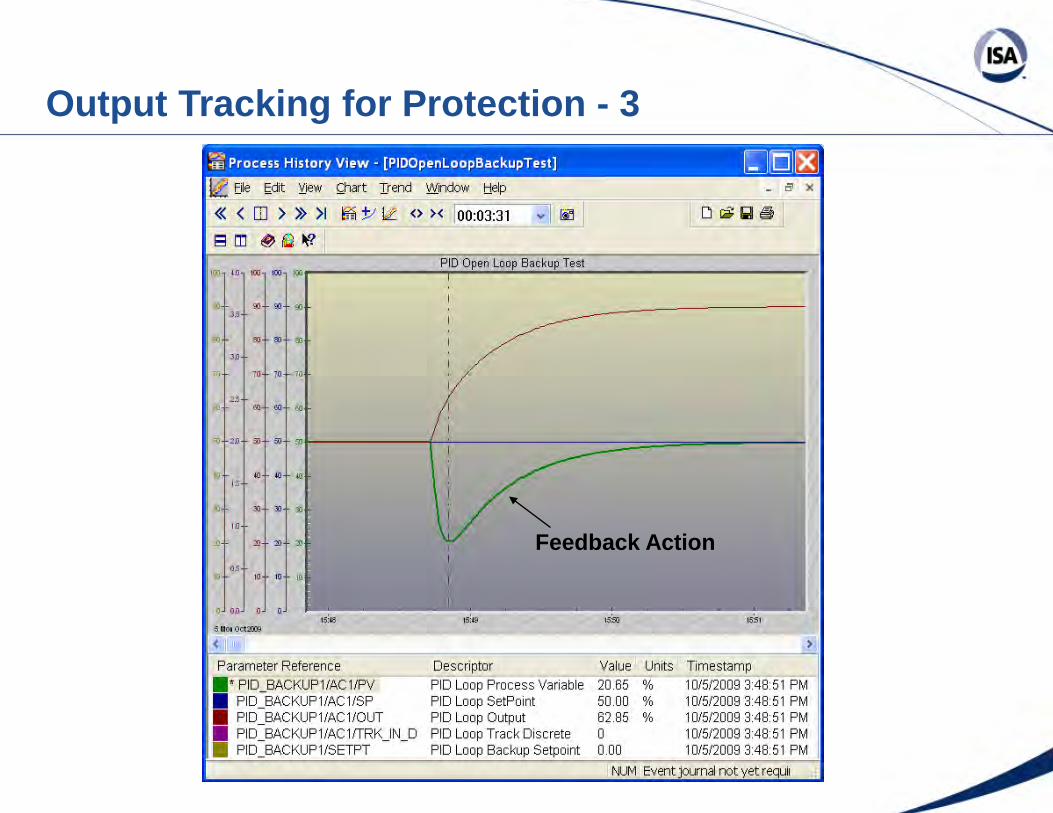
Output Tracking for Protection - 3

Feedback Action

Open Loop Backup

Output Tracking for Protection - 4

Mixer

Attenuation Tank

AY

AT

middle selector

AY splitter

AT

FT

FT

AT

AY

AT AT AT

AY

AT AT AT

Mixer

AY

FT

Stage 2 Stage 1

middle selector

Waste middle selector RCAS RCAS

splitter

AY

Filter

AY ROUT Kicker AC-1 AC-2

MPC-2

MPC-1

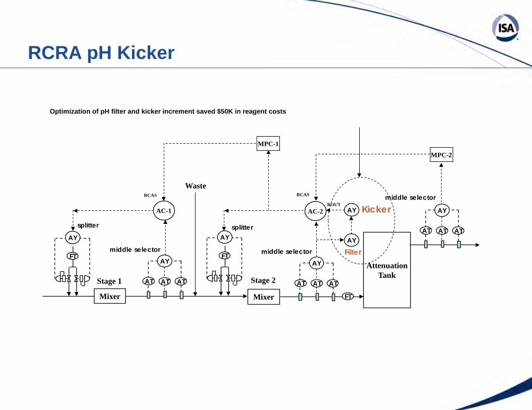
RCRA pH Kicker

Optimization of pH filter and kicker increment saved $50K in reagent costs

Evaporator Conductivity Kicker

Conductivity spike

WBL Flow Kicker

Setpoint Filter

• PID SP filter reduces overshoot enabling fast tuning – Setpoint filter time set equal reset time

• PID SP filter coordinates timing of flow ratio control – Simultaneous changes in feeds for blending and reactions – Consistent closed loop response for model predictive control

• PID SP filter sets closed loop time constant • PID SP filter in secondary loop slows down cascade control

system rejection of primary loop disturbances – Secondary loop must be > 4x faster than primary loop

• Primary PID must have dynamic reset limit enabled • Setpoint Lead-Lag minimizes overshoot and rise time

– Lag time = reset time – Lead time = 20% lag time

Setpoint Rate Limits

• AO & PID SP rate limits minimize disruption while protecting equipment and optimizing processes – Offers directional moves suppression – Enables fast opening and slow closing surge valve – VPC fast recovery for upset and slow approach to optimum

• AO SP rate limits minimize interaction between loops – Less important loops are made 10x slower than critical loops

• PID driving AO SP or secondary PID SP rate limit must have dynamic reset limit enabled so no retuning is needed

• PID faceplate should display PV of AO to show rate limiting

Top Ten Reasons to do APC from your Home

• (10) Can immediately implement an inspiration.

• (9) Can watch the ball game on one of your screens.

• (8) Get to wear shorts and sandals.

• (7) Get to listen to music rather than alarms.

• (6) Lose weight from not eating doughnuts.

• (5) Can BBQ while solving control problem.

• (4) No more lonely nights and meals.

• (3) Your kids start to recognize you.

• (2) Your kids want to become automation engineers.

• (1) Your spouse starts to offer you advanced process control.

63

Enhanced PID for Wireless Features

• Positive feedback implementation of reset with external-reset feedback (dynamic reset limit)

• Immediate response to a setpoint change or feedforward signal or mode change

• Suspension of integral action until change in PV • Integral action is the exponential response of the positive feedback

filter to the change in controller output in elapsed time (the time interval since last update)

• Derivative action is the PV or error change divided by elapsed time rather than PID execution

Traditional PID Sensor PV

Enhanced PID Sensor PV

Flow Setpoint Response

Traditional PID Sensor PV

Enhanced PID Sensor PV

Flow Load Response

Enhanced PID Sensor PV

Traditional PID Sensor PV

Flow Signal Failure Response

Enhanced PID Sensor PV

Traditional PID Sensor PV

pH Setpoint Response

Traditional PID Sensor PV

Enhanced PID Sensor PV

pH Load Response

Traditional PID Sensor PV

Enhanced PID Sensor PV

pH Sensor Failure Response

PID PV

PID Output

Enhanced PID Traditional PID

Limit Cycles from Valve Stick-Slip

Stop Limit Cycles

• The PID enhancement for wireless offers an improvement wherever there is an update time in the loop. In the broadest sense, an update time can range from seconds (wireless updates and valve or measurement sensitivity limits) to hours (failures in communication, valve, or measurement). Some of the sources of update time are: – Wireless update time for periodic reporting (default update rate) – Wireless measurement trigger level for exception reporting (trigger level) – Wireless communication failure – Broken pH electrode glass or lead wires (failure point is about 7 pH) – Valve with backlash (deadband) and stick-slip (resolution) – Operating at split range point (no response & abrupt response discontinuity) – Valve with solids, high temperature, or sticky fluid (plugging and seizing) – Plugged impulse lines – Analyzer sample, analysis cycle, and multiplex time – Analyzer resolution and threshold sensitivity limit

To completely stop a valve limit cycle from backlash or stick-slip,

measurement updates must not occur due to noise

Benefits Extend Beyond Wireless - 1

• Enhanced PID executes for a change in setpoint, feedforward, or remote output to provide an immediate reaction based on PID structure

• The improvement in control by the enhanced PID is most noticeable as the update time becomes much larger than the 63% process response time (defined in the white paper as the sum of the process deadtime and time constant). When the update time becomes 4 times larger than this 63% process response time ( 98% response time frequently cited in the literature), the feedforward and controller gains can be set to provide a complete correction for changes in the measurement and setpoint. – Helps ignore inverse response and errors in feedforward timing – Helps ignore discontinuity (e.g. steam shock) at split range point – Helps extend packing life by reducing oscillations and hence valve travel

• Since enhanced PID can be set to execute only upon a significant change in user valve position, this PID as a valve position controller offers less interaction and cycling for optimization of unit operations by increasing reactor feed, column feed or increasing refrigeration unit temperature, or decreasing compressor pressure till feed, vent, coolant, and/or steam, valves are at maximum good throttle position.

http://www.modelingandcontrol.com/2010/08/wireless_pid_benefits_extend_t.html http://www.modelingandcontrol.com/2010/10/enhanced_pid_for_wireless_elim.html

http://www.modelingandcontrol.com/2010/11/a_delay_of_any_sorts.html

Website entries on Enhanced PID Benefits

Benefits Extend Beyond Wireless - 2

Why over 100 PID Tuning Rules?

• Aidan O’Dwyer’s Handbook of PI and PID Controller Tuning Rules - 2nd Edition has over 500 pages of rules

• The originators all think their rules are best due to – Gamesmanship – Diverse sources of change – Diverse objectives – Diverse dynamics – Diverse metrics

Convergence of Tuning Rules

• The most popular PID rules converge to the same equations for 99% of temperature, composition, level, and gas pressure loops despite diversity of metrics, dynamics, objectives, and sources of change if the following is used: – Tuning to minimize the effect of unmeasured disturbances – Tuning to maximize absorption of variability (e.g. surge tank level) – Dead time block in identification of process dynamics – Primary PID Setpoint Lag = reset time and Lead = 20% of Lag – Analog output setpoint rate limit and PID external-reset feedback – Enhanced PID developed for wireless with threshold sensitivity

• For the remaining cases: – For drastic deceleration from dead time dominance decrease gain,

reset time, and rate time – For severe acceleration from runaway reaction, increase gain,

reset time, and rate time

Diverse Sources of Change

• Raw material and recycle composition and impurities • Weather (temperature, humidity, snow, rain) • Utility temperature and pressure • Operators (production rate changes and manual actions) • Interactions and Optimization • Batch sequences and on-off control • Startups, transitions, and shutdowns • Measurement and process noise • Limit cycles

Diverse Process Objectives

• Maximize safety – Prevent activation of relief devices and Safety Instrumented

Systems (SIS) • Maximize equipment, environmental, & process protection • Minimize product variability

– Minimize limit cycles – Minimize oscillatory loop response – Minimize interaction between loops – Maximize coordination between loops

• Maximize process capacity and efficiency – Increase production rate and decrease raw material and utility use

Diverse Process Objectives Automated Risk Reduction

PID

SIS

Diverse Process Objectives Maximize Protection

• Eliminate temperature shock and water hammer – Slow action of control valve in direction of causing shock

• Eliminate compressor surge – Slow closing of surge valves and downstream user valves – Fast opening of surge valves

• Eliminate flare stack emissions – Fast opening of runaway reactor coolant valves

• Eliminate RCRA pH Violations – Fast opening of base reagent valve when approaching 2 pH – Fast opening of acid reagent valve when approaching 12 pH

Diverse Process Objectives Minimize Product Variability

• Minimize cycling from valve discontinuities – Suspension of integral action when valve is not moving or for an

impending unnecessary crossing of the split range point • Minimize oscillatory response

– Slow approach to setpoint and suspension of integral action between updates from analyzers and wireless transmitters

• Minimize interaction between loops – Slow and fast action of less and more critical loop, respectively

• Maximize coordination of loops – Identical ratioed rates of change of feeds particularly for plug flow

reactors, and inline systems, such as blenders and static mixers

Diverse Process Objectives Maximize Efficiency and Capacity

• Use PID for valve position control (VPC) to increase feed or reduce raw material or energy use for valve constraint. – Slow approach by VPC to optimum to avoid upsetting loops – Fast getaway by VPC for upset to avoid running out of valve – Suspension of integral action in VPC for valve that is not moving or

whose movements are inconsequential

Key PID Features for VPC

Feature Function Advantage 1 Advantage 2

Direction Velocity Limits

Limit VPC Action Speed Based on

Direction

Prevent Running Out of Valve

Minimize Disruption to Process

Dynamic Reset Limit

Limit VPC Action Speed to Process

Response

Direction Velocity Limits

Prevent Burst of Oscillations

Adaptive Tuning Automatically Identify and Schedule Tuning

Eliminate Manual Tuning

Compensation of Nonlinearity

Feedforward Preemptively Set VPC Out for Upset

Prevent Running Out of Valve

Minimize Disruption

Enhanced PID (PIDPlus)

Suspend Integral Action until PV Update

Eliminate Limit Cycles from Stiction &

Backlash

Minimize Oscillations from Interaction & PV

Update Delay

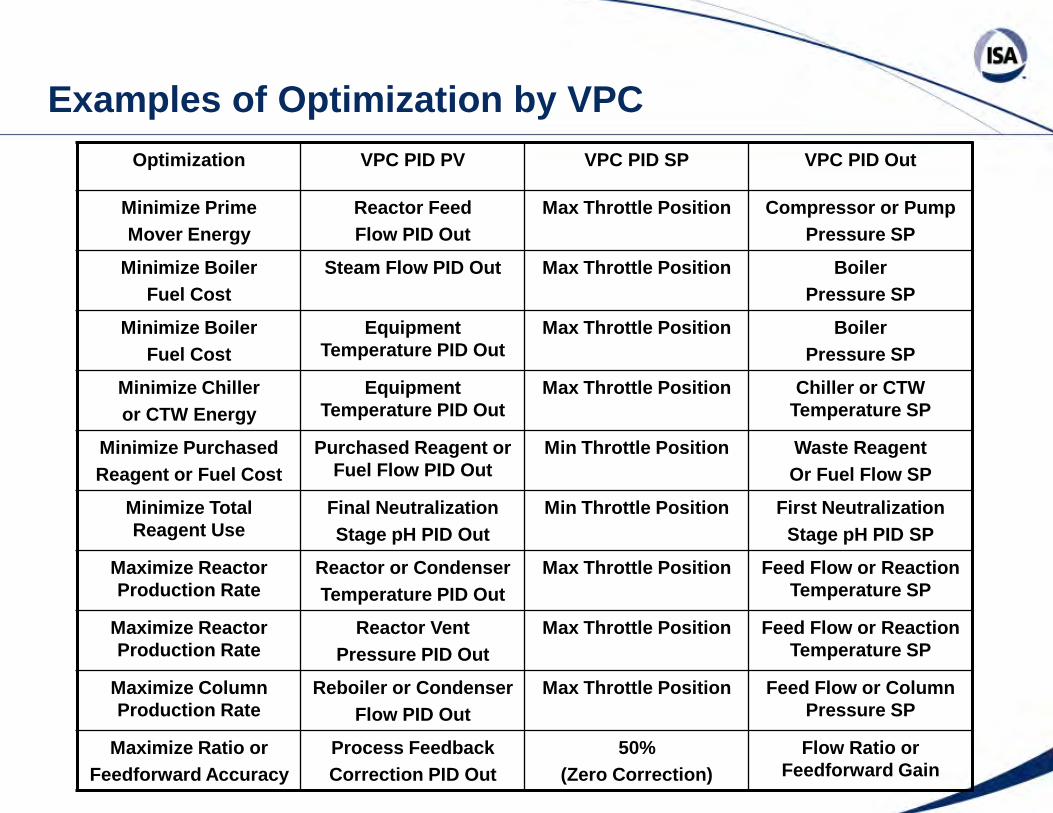
Examples of Optimization by VPC Optimization VPC PID PV VPC PID SP VPC PID Out

Minimize Prime Mover Energy

Reactor Feed Flow PID Out

Max Throttle Position Compressor or Pump Pressure SP

Minimize Boiler Fuel Cost

Steam Flow PID Out Max Throttle Position Boiler Pressure SP

Minimize Boiler Fuel Cost

Equipment Temperature PID Out

Max Throttle Position Boiler Pressure SP

Minimize Chiller or CTW Energy

Equipment Temperature PID Out

Max Throttle Position Chiller or CTW Temperature SP

Minimize Purchased Reagent or Fuel Cost

Purchased Reagent or Fuel Flow PID Out

Min Throttle Position

Waste Reagent Or Fuel Flow SP

Minimize Total Reagent Use

Final Neutralization Stage pH PID Out

Min Throttle Position

First Neutralization Stage pH PID SP

Maximize Reactor Production Rate

Reactor or Condenser Temperature PID Out

Max Throttle Position Feed Flow or Reaction Temperature SP

Maximize Reactor Production Rate

Reactor Vent Pressure PID Out

Max Throttle Position Feed Flow or Reaction Temperature SP

Maximize Column Production Rate

Reboiler or Condenser Flow PID Out

Max Throttle Position Feed Flow or Column Pressure SP

Maximize Ratio or Feedforward Accuracy

Process Feedback Correction PID Out

50% (Zero Correction)

Flow Ratio or Feedforward Gain

84

Liquid Reactants (Jacket CTW) Liquid Product Optimization

TT 1-4

TC 1-3

TC 1-4

AT 1-6

LY 1-8

FY 1-6

FT 1-2

FC 1-2

reactant A

reactant B

CAS

residence time calc

CAS

ratio calc

AC 1-6

makeup

return

LY 1-8

FY 1-6

reactant A

reactant B

residence time calc LT

1-8 TT 1-3

LC 1-8

ratio calc

product

vent FT 1-1

FC 1-1

FC 1-1 CAS

ZC1-4 OUT

ZC 1-4

FC 1-7

FT 1-7

PT 1-5

PC 1-5

FT 1-5

CTW

ZC1-4 is an enhanced PID VPC

Valve position controller (VPC) setpoint is the maximum throttle position. The VPC should turn off integral action to prevent interaction and limit cycles. The correction for a valve position less than setpoint should be slow to provide a slow approach to optimum. The correction for a valve position greater than setpoint must be fast to provide a fast getaway from the point of loss of control. Directional velocity limits in AO with dynamic reset limit in an enhanced PID that tempers integral action can achieve these optimization objectives.

85

Liquid Reactants (Jacket CTW) Gas & Liquid Products Optimization

TT 1-4

TC 1-4

AT 1-6

LY 1-8

FY 1-6

FT 1-2

FC 1-2

reactant A

reactant B

residence time calc

CAS

ratio calc

AC 1-6

makeup

return

LY 1-8

FY 1-6

reactant A

reactant B

CAS

residence time calc LT

1-8

LC 1-8

ratio calc

product

FT 1-1

FC 1-1

FC 1-7

FT 1-7

CAS

TC 1-3

TT 1-3

product

PC 1-5

FT 1-5

W

PT 1-5

TT 1-10

TC 1-10

ZC 1-4

ZC 1-10

ZC 1-5

ZY 1-1

FC1-1 CAS

ZY1-1 OUT

low signal selector

ZC-10 OUT

ZC-4 OUT

ZC-5 OUT

ZY-1 IN1

ZY-1 IN2

ZY-1 IN3

CTW

ZC1-4, ZC-5, & ZC-10 are enhanced PID VPC

86 86

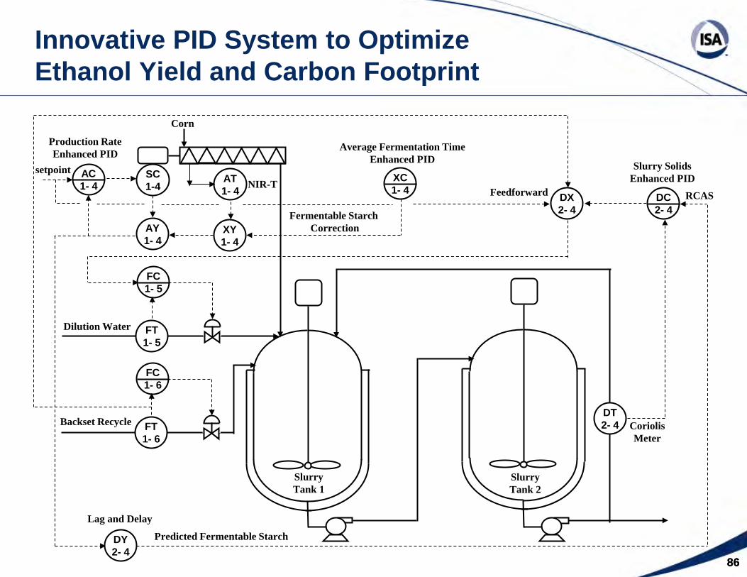
Innovative PID System to Optimize Ethanol Yield and Carbon Footprint

AT 1- 4

AC 1- 4

DC 2- 4

SC 1-4

FT 1- 5

FC 1- 5

AY 1- 4

Corn

NIR-T

Production Rate Enhanced PID

DT 2- 4

Slurry Solids Enhanced PID

DX 2- 4

Feedforward

FT 1- 6

FC 1- 6

Backset Recycle

Dilution Water

XC 1- 4

XY 1- 4

Average Fermentation Time Enhanced PID

Fermentable Starch Correction

Slurry Tank 1

Slurry Tank 2

Coriolis Meter

setpoint

DY 2- 4

Lag and Delay

RCAS

Predicted Fermentable Starch

87

Loop Block Diagram (First Order Approximation)

τs θp τp Kp θs

τc1 τm2 θm2 τm1 θm1 Km θc τc2

Kc Ti Td

Valve Process

Controller Measurement

Kv τv θv

Kd τL θd

Load Upset

∆%PV

∆%CO

∆Fv ∆PV

PID

Delay Lag

Delay Secondary

Delay Primary Delay

Delay

Delay

Delay

Lag Secondary

Lag Primary

Lag

Lag Lag Lag

Lag

Gain

Gain

Gain

Gain

Local Set Point

%SP

∆DV

First Order Approximation: θο ≅ θv + θs + θp + θm1 + θm2 + θc + Y∗τv + Y∗τs + Y∗τm1 + Y∗τm2 + Y∗τc1 + Y∗τc2 (set by automation system design for flow, pressure, level, speed, surge, and static mixer pH control)

%

%

%

Delay <=> Dead Time Lag <=>Time Constant

For self-regulating processes: Ko = Kv ∗ Kp ∗ Km For near integrating processes: Ki = Kv ∗ (Kp / τp) ∗ Km

Km = 100% / span

τo is the largest lag in the loop (hopefully τp)

½ of Wireless Default Update Rate

Kv = slope of installed flow characteristic

88

Open Loop Response of Self-Regulating Process

Time (seconds)

∆%CO

∆%PV

θo

Ko = ∆%PV / ∆%CO

0.63∗∆%PV

%CO

%PV

Self-regulating process open loop negative feedback time constant

Self-regulating process gain (%/%)

Response to change in controller output with controller in manual

observed total loop dead time

ideally τp τo

Maximum speed in 4 dead times

is critical speed

Noise Band

% P

roce

ss V

aria

ble

(%PV

) or

%

Con

trol

ler O

utpu

t (%

CO

)

89

Open Loop Response of Integrating Process

Time (seconds) θo

Ki = { [ %PV2 / ∆t2 ] − [ %PV1 / ∆t1 ] } / ∆%CO

∆%CO

ramp rate is ∆%PV1 / ∆t1

ramp rate is ∆%PV2 / ∆t2

%CO

%PV

Integrating process gain (%/sec/%)

Response to change in controller output with controller in manual

observed total loop dead time

Maximum ramp rate in 4 dead times is used to estimate integrating

process gain

% P

roce

ss V

aria

ble

(%PV

) or

%

Con

trol

ler O

utpu

t (%

CO

)

90

Open Loop Response of Runaway Process

Response to change in controller output with controller in manual

Noise Band

Acceleration

∆%PV

∆%CO

1.72∗∆%PV

Ko = ∆%PV / ∆%CO Runaway process gain (%/%)

% P

roce

ss V

aria

ble

(%PV

) or

%

Con

trol

ler O

utpu

t (%

CO

)

Time (seconds) observed total loop dead time runaway process open loop

positive feedback time constant

For safety reasons, tests are terminated within 4 dead times before noticeable acceleration

τ’ o must be τ’ p θo

Diverse Loop Metrics

• Peak and integrated errors for load disturbances • Rise time for setpoint change (time to reach setpoint) • Overshoot for setpoint change • Settling time for setpoint change • Standard deviation of oscillations

Diverse Metrics Peak and Integrated Error

The use of a setpoint lead-lag with the lag equal to the reset time and the lead 20% of the lag will provide a fast setpoint response with minimal overshoot

despite tuning for maximum load rejection

ooo

ox EE ∗

+=

)( τθθ

ooo

oi EE ∗

+=

)(

2

τθθ

Peak error is proportional to the ratio of loop dead time to 63% response time (Important to prevent SIS trips, relief device activation, surge prevention, and RCRA pH violations)

Integrated error is proportional to the ratio of loop dead time squared to 63% response time (Important to minimize quantity of product off-spec and total energy and raw material use)

For a sensor lag (e.g. electrode or thermowell lag) or signal filter that is much larger than the process time constant, the unfiltered actual process variable error can be

found from the equation for attenuation

Ultimate Limit to Loop Performance

Total loop deadtime that is often set by automation design

Largest lag in loop that is ideally set by large process volume

Effect of Disturbance Lag on Integrating Process

Periodic load disturbance time constant increased by factor of 10

Adaptive loop

Baseline loop Adaptive loop

Baseline loop

Primary reason why bioreactor control loop tuning and performance for load upsets is a non issue!

oco

x EKK

E ∗∗+

=)1(

1

oco

fxii E

KKtT

E ∗∗

+∆+=

τ

Peak error decreases as the controller gain increases but is essentially the open loop error for systems when total dead time >> process time constant

Integrated error decreases as the controller gain increases and reset time decreases but is essentially the open loop error multiplied by the reset time plus signal delays and lags for systems when total dead time >> process time constant

Peak and integrated errors cannot be better than ultimate limit - The errors predicted by these equations for the PIDPlus and deadtime compensators cannot be better

than the ultimate limit set by the loop deadtime and process time constant

Practical Limit to Loop Performance

Open loop error for fastest and largest load disturbance

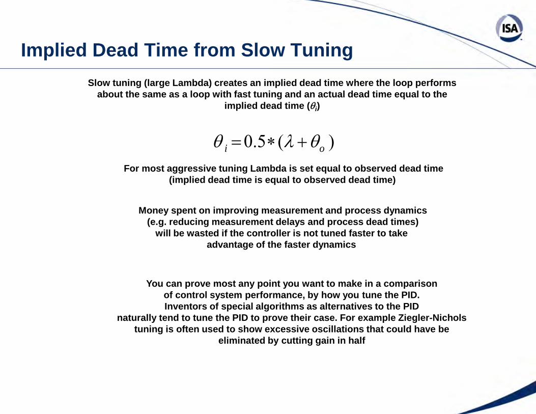
)(5.0 oi θλθ +∗=

Slow tuning (large Lambda) creates an implied dead time where the loop performs about the same as a loop with fast tuning and an actual dead time equal to the

implied dead time (θi)

Implied Dead Time from Slow Tuning

For most aggressive tuning Lambda is set equal to observed dead time (implied dead time is equal to observed dead time)

Money spent on improving measurement and process dynamics (e.g. reducing measurement delays and process dead times)

will be wasted if the controller is not tuned faster to take advantage of the faster dynamics

You can prove most any point you want to make in a comparison of control system performance, by how you tune the PID. Inventors of special algorithms as alternatives to the PID

naturally tend to tune the PID to prove their case. For example Ziegler-Nichols tuning is often used to show excessive oscillations that could have be

eliminated by cutting gain in half

oL EeE Lo ∗−= − )1( /τθ

Effect of load disturbance lag (τL) on peak error can be estimated by replacing the open loop error with the exponential response of the disturbance during the loop dead time

Disturbance Speed

For Ei (integrated error), use closed loop time constant instead of dead time

For a load disturbance lag much larger than the dead time, the load error in one dead time Is very small, allowing a very large implied dead time from slow tuning. In other words,

tuning and control loop dynamics are not important in terms of disturbance rejection. The focus is then on the effect of tuning and dynamics on rise time (time to reach a new setpoint)

Setpoint Response Rise Time

Rise time (time to reach a new setpoint) is inversely proportional to controller gain

offci

r SPKKCOKSPT θ+

∆∗+∆∗∆

=)%)(|,%|(min

%

max

Rise time can be decreased by setpoint feedforward and bang-bang logic that sets and holds an output change at maximum (∆%COmax) for one dead time until future PV value is projected to reach setpoint. The fastest possible rise time is:

oi

r COKSPT θ+

∆∗∆

=|%|

%

max

Basic Lambda Tuning (Self-Regulating Processes)

COPV

Ko %%

∆∆

=

)( oo

ic K

TKθλ +∗

=

oiT τ=

Self-Regulation Process Gain:

Controller Gain

Controller Integral Time

of τλλ ∗=Lambda (Closed Loop Time Constant for Setpoint Response)

Lambda tuning excels at coordinating loops for blending, fixing lower loop dynamics for model predictive control,

and reducing loop interaction and resonance

Fastest Lambda Tuning (Self-Regulating Process)

oθλ =

For max load rejection set lambda equal to dead time

oo

oc K

Kθ

τ∗

∗= 5.0

oiT τ=

Basic Lambda Tuning Integrating Processes

Integrating Process Gain:

Controller Gain:

Controller Integral (Reset) Time:

Lambda (closed loop arrest time in load response)

if K/λλ =

COtPVtPV

Ki %/%/% 1122

∆∆∆−∆∆

=

2][ oi

ic K

TKθλ +∗

=

oiT θλ +∗= 2

Controller Derivative (Rate) Time:

sdT τ= secondary lag

Fastest Lambda Tuning Integrating Processes

Controller Gain:

Controller Integral (Reset) Time:

oic K

Kθ∗∗

=43

oiT θ∗= 3

Controller Derivative (Rate) Time:

sdT τ= secondary lag

oθλ =For max load rejection set lambda equal to dead time

Check for prevention of slow rolling oscillations:

iic K

TK 25.2* =

103

To prevent slow rolling oscillations:

iic K

TK 2* >

Often Violated Criteria for Integrating Processes

Near Integrator Approximation (Short Cut Method)

]%/)/%[( COtPVMaxKKp

oi ∆∆∆==

τ

For “Near Integrating” gain approximation use maximum ramp rate divided by change in controller output

Compute maximum ramp rate as maximum delta between input (new %PV) and output (old %PV) of dead time block divided by the block dead time

and finally the change in controller output (block dead time is total loop dead time)

CO

PV

K oi %

% max

∆

∆

=θ

Estimate open loop gain as the difference between current operating point and original operating point

o

oo COCO

PVPVK%%%%

−−

=

oo

oc K

Kθ

τ∗

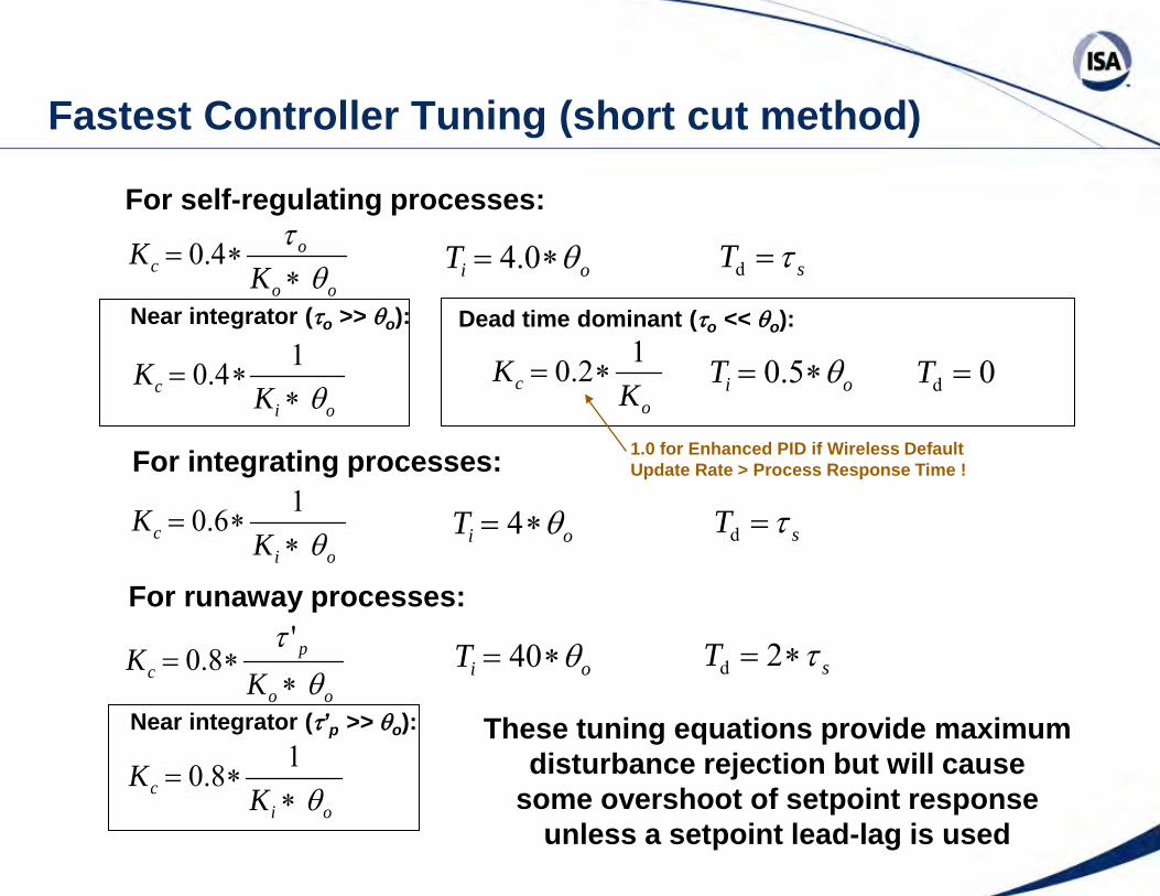
∗= 4.0 oiT θ∗= 0.4 sT τ=d

For runaway processes:

For self-regulating processes:

oic K

Kθ∗

∗=16.0 oiT θ∗= 4 sT τ=d

oic K

Kθ∗

∗=18.0

oiT θ∗= 40 sT τ∗= 2d

For integrating processes:

oo

pc K

Kθ

τ∗

∗='

8.0

oic K

Kθ∗

∗=14.0

Near integrator (τo >> θo):

oiT θ∗= 5.0

Near integrator (τ’p >> θo):

Dead time dominant (τo << θo):

0d =To

c KK 12.0 ∗=

Fastest Controller Tuning (short cut method)

These tuning equations provide maximum disturbance rejection but will cause

some overshoot of setpoint response unless a setpoint lead-lag is used

1.0 for Enhanced PID if Wireless Default Update Rate > Process Response Time !

Top Ten Things Missing in University Courses on Process Control

• (10) Control valves with stick-slip and deadband

• (9) Measurements with repeatability errors and turndown limits

• (8) Volumes with variable mixing and transportation delays

• (7) Process input load disturbance

• (6) Control action (direct & reverse) & valve action (increase-open & increase-close)

• (5) PID algorithms using percent

• (4) PID structure, anti-reset windup, output limits, and dynamic reset

• (3) Industry standards for function blocks and communication

• (2) “Control Talk”

• (1) My books

Ultimate Period and Ultimate Gain

Time (min)

Measurement (%)

Ultimate Gain is Controller Gain that Caused these Nearly Equal Amplitude Oscillations (Ku)

Set Point

Ultimate Period Tu

0

If τo >> θo then Tu = 4 ∗ θ If τo << θo then Τu = 2 ∗ θ

Set Point

Time (min)

Measurement (%)

Offset

110% of θo

Quarter Amplitude Period To

0

Damped Oscillation - (Proportional-Derivative)

1. Put the controller in auto at normal setpoint. 2. Choose largest step change in controller setpoint that is safe. Increase the reset time

by a factor of 10x for test. 3. Add a PV filter to keep the controller output fluctuations from noise within the valve

deadband. 4. Step the controller setpoint. If the response is non-oscillatory, increase the controller

gain and step the controller setpoint in opposite direction. Repeat until you get a slight oscillation (ideally ¼ amplitude decay). Make sure the controller output is not hitting the controller output limits and is on the sensitive part of the control valve’s or variable speed drive’s installed flow characteristic.

5. Estimate the period of the oscillation. Reduce the controller gain until the oscillation disappears (½ current gain), set the reset time equal to ½ the period, and the rate time equal to ¼ of the reset time. If the oscillation is noisy or resembles a square wave or the controller gain is high (e.g. > 10), set the rate time to zero. The factors are ½ the ultimate period and twice the ultimate gain factors because the controller gain that triggered the ¼ amplitude oscillation is about ½ the ultimate gain and the ¼ amplitude period is larger than the ultimate period.

6. If a high controller gain is used (e.g. > 10) use AO setpoint rate of change (velocity) limits if a big kick in the controller output for setpoint changes is disruptive to operations from PD action on error (enable external reset feedback).

7. Make setpoint changes across the range of operation to make sure an operating point with a higher controller gain or larger process dead time does not cause oscillations. Monitor the loop closely over several days of operation.

Damped Oscillation Tuning Method

Traditional Open Loop Tuning Method 1. Choose largest step change in controller output that is safe. 2. Add a PV filter to keep the controller output fluctuations from noise within the valve

deadband. 3. Make a change in controller output in manual. 4. Note the time it take for the process variable to get out of the noise band as the loop

dead time. 5. Estimate the process time constant as the time to reach 63% of the final value. 6. Estimate the process gain as final change in the process variable (%) after it reaches a

steady state divided by change in the controller output (%). 7. To use reaction curve tuning, set the controller gain equal to ½ the process time

constant divided by the product of the process gain and dead time. 8. If the process lag is much larger than the loop dead time, set the reset time setting

equal to 4x the dead time and set the rate time setting equal to the dead time. If process lag is much smaller than the loop dead time, set the reset time to 0.5x the loop dead time and the rate time to zero.

9. If a high controller gain is used (e.g. > 10) use setpoint rate of change (velocity) limits if a big kick in the controller output for setpoint changes is disruptive to operations for PD on error (enable external reset feedback).

10. Make setpoint changes across the range of operation to make sure an operating point with a higher controller gain or larger process dead time does not cause oscillations. Monitor the loop closely over several days of operation.

Short Cut Ramp Rate Tuning Method

1. Choose largest step change in controller output and setpoint that is safe. If the test is to be made in auto, increase the reset time by factor of 10x for test.

2. Add a PV filter to keep the controller output fluctuations from noise within the valve deadband. Measure the initial rate of change of the process variable (∆PV1/∆t).

3. Make a either a change in controller output in manual or change in set point in auto 4. Note the time it take for the for the process variable to get out of the noise band as the

loop dead time. 5. Estimate the rate of change of the process variable (∆PV2/∆t) over successive dead time

intervals (at least two). Choose the largest rate of change. Subtract this from initial rate of change of the process variable and divide the result by the step change in controller output to get the integrating process gain.

6. Set the controller gain equal to the inverse of the product of integrating process gain and loop dead time multiplied by 0.4 (self-regulating), 0.6 (integrating), and 0.8 (runaway) • If the inverse of the integrating gain is much larger than the loop dead time, set the reset time

setting equal to 4x the process dead time and set the rate time setting equal to the process dead time, otherwise set the reset time to 0.5x the process dead time and the rate time to zero

7. If a high controller gain is used (e.g. > 10) use setpoint rate of change (velocity) limits if a big kick in the controller output for setpoint changes is disruptive to operations from PD action on error (enable external reset feedback).

8. Make setpoint changes across the range of operation to make sure an operating point with a higher controller gain or larger process dead time does not cause oscillations. Monitor the loop closely over several days of operation.

On-Demand Tuning Algorithm

Time (min)

Ultimate Period Tu

0

Set Point

d

a

Ultimate Gain 4 ∗ d Ku = −−−− π ∗ e

n

e = sq rt (a2 - n2) If n = 0, then e = a alternative to n is a filter to smooth PV

Signal (%)

Adaptive Tuning Algorithm

Pure Gain Process

K

Estimated Gain

Multiple Model Interpolation with Re-centering

K

Estimated Gain

Multiple Model Interpolation with Re-centering

Changing Process Input

2( ) ( ( ) ( ) ) iE t y t Yi t= −

For each iteration, the squared error is computed for every model I each scan

Where:is the process output at the time tis i-th model output

A norm is assigned to each parameter value k = 1,2,….,m in models l = 1,2,…,n.

if parameter value is used inthe model, otherwise is 0

For an adaptation cycle of M scans

( ) y t( ) Yi t

1

( ) ( ) N

klkl i

i

Ep t E tγ=

= ∑= 1klγ

klp

1

( )M

kl kl

t

sumEp Ep t=

= ∑

1kl

kk

Ff sumF=

1kl klF

sumEp=

11( ) ... ...k k kl kn

k kl knp a p f p f p f= + + + +

Initial Model Gain = G1

G2-Δ G2 G2+ΔG2-Δ G2 G2+Δ

G3-Δ G3 G3+ΔG3-Δ G3 G3+Δ

Multiple iterations per

adaptation cycle

The interpolated parameter value is

Broadley-James Corporation Bioreactor Setup

• Hyclone 100 liter Single Use Bioreactor (SUB)

• Rosemount WirelessHART gateway and transmitters for measurement and control of pH and temperature. (pressure monitored)

• BioNet lab optimized control system based on DeltaV

Bioreactor Adaptive Control Performance

Bioreactor Adaptive Tuning Setup

Bioreactor Adaptive Model Viewing

Bioreactor Adaptive Learning Setup

Output comes off high limit at 36.8 oC

0.30 oC overshoot

Bioreactor Adaptive Tuning Gain 40 Reset 500

Output comes off high limit at 35.9 oC

0.12 oC overshoot

Bioreactor Adaptive Tuning Gain 40 Reset 5,000

0.13 oC overshoot

Output comes off high limit at 36.1 oC

Bioreactor Adaptive Tuning Gain 40 Reset 10,000

0.20 oC overshoot

Output comes off high limit at 36.4 oC

Bioreactor Adaptive Tuning Gain 40 Reset 15,000

0.11 oC overshoot

Output comes off high limit at 36.1 oC

Bioreactor Adaptive Tuning Gain 80 Reset 15,000

Integrating and Runaway Process Tuning

• It is difficult to prevent overshoot in processes without self-regulation • Controller gain adds self-regulation via closed loop response • Examples of integrating processes (ramping response) are

– Liquid and solids level – furnace, column, or vessel pressure – batch composition, pH, or temperature

• Examples of runaway processes (accelerating response) are – exothermic reactor temperature – strong acid - strong base pH – exponential growth phase biomass – compressor speed during surge

• An overdrive of the controller output beyond its resting value is needed to reach a set point or compensate for a disturbance (achieved by high controller gain)

• The maximum allowable controller gain for many integrating processes is well beyond the comfort level of most users. Measurement noise and resolution often sets the practical high limit to the controller gain rather than process dynamics

• Too much reset action (too small of a reset time) cause severe overshoot • A higher controller gain creates more overdrive for small setpoint changes and

gets controller off it’s output limit sooner for large setpoint changes • There is a window of allowable controller gains.

– Instability from too high of a controller gain (not likely for industrial processes) – Slow rolling oscillations from too low of a controller gain (common case) that slowly

decay for integrating processes but can grow for runaway till it hits physical limits

Arrest Time for Max Variability Absorption - 1 The arrest time ( λ) is the max allowable % excursion (∆%PVmax) divided by the max PV ramp rate. The max ramp rate is the PV rate of change per % output change multiplied by the max available % output change (∆%COmax).

max

max

%

%

%

%

CO

COtPV

PV

∆∗

∆∆

∆

∆=λ

Realizing that the integrating process gain is the PV rate of change per percent output change:

max

max

%%1

COPV

Ki ∆∆

∗=λ

For a PV limit (%PVmax) and corresponding CO limit (%COmax) we have

COCOSPPV

K Limit

Limit

i %%%%1

−−

∗=λ

The above calculation would be done for high and low operating limits and various setpoints. The smallest of the arrest times would be used in tuning.

The integrating process gain is the product of the valve, process, and measurement gains:

mpvi KKKK ∗∗=

The valve gain or variable speed drive gain for a linear installed characteristic or flow loop is:

%100%maxF

COFK v

v∆

=∆

∆=

The level process gain for mass flow is (omit density term for volumetric flow):

ρ∗=

AK p

1

The level measurement gain is:

max

%100%LL

PVKm ∆=

∆∆

=

Arrest Time for Max Variability Absorption - 2

Substituting in the valve, process, and measurement gains, the integrating process gain is:

ρρ ∗∗

∆∆

=∆

∗∗

∗∆

=∗∗=AL

FLA

FKKKK mpvi1%1001

%100 max

max

max

max

The consequential arrest time for a level loop is:

max

max

max

max

%%

COPV

FLA

∆∆

∗∆

∆∗∗=

ρλ

An equivalent setpoint rate limit on the controller output (e.g. flow controller setpoint):

max

2max

max

maxmax

max %%%%

PVCO

LAFCO

tCO

∆∆

∗∆∗∗

∆=

∆=∆

∆ρλ

Arrest Time for Max Variability Absorption - 3

Simplified Approach for Diverse Applications and Requirements

• Use lambda integrator tuning rules for integrating, runaway, and lag dominant self-regulating processes – For maximum disturbance rejection set arrest time = dead time (λ = θo) – To absorb variability compute arrest time (λ) from integrating process gain,

allowable ∆%PVmax excursion, and available ∆%COmax per last slide – Compute controller gain and reset time based on selected arrest time – Set rate time equal to secondary time constant

• Use external-reset feedback (dynamic reset limit) • Use setpoint filter and rate limits (directional move suppression)

to improve coordination, optimization, and reduce interaction • Use enhanced PID to eliminate oscillations from valve backlash

or stiction, split range point, interaction, or large and variable update time (e.g., at-line or offline analyzers)

• Use output tracking for equipment protection and bang-bang logic • Use feedforward for fast and large measured disturbances

129

Effect of Wireless Measurement Update Time and Interval on Performance

o

omS E

S τθ ∗∗=

5.0

ovwo

x ET

E ∗++

=63

θθθo

vwoi E

TE ∗

++=

63

2)( θθθowoT τθθ ++=63

),( STw Min θθθ ∆= wT T∆∆ ∗= 5.0θmax)/%(

5.0tPV

SmS ∆∆

∗=θ

)/()/%( max ooi KEKtPV ∗=∆∆o

oi

KKτ

=o

oE

tPVτ

=max)/%( ∆∆

130

Additional Dead Time from Valve Stick-Slip, Resolution, or Deadband

ox

oovv EK

KS∗

∗∗∗=

θθ 5.0

max)/%(5.0

tCOSv

v ∆∆∗

=θ maxmax )/%()/%( tPVKtCO c ∆∆∆∆ ∗=

oo

x

KEK

tCO o

θ∗

∗=max)/%( ∆∆

[ ]

−∗

∗=

002.0),(max,min

mm

v

oo

oxc SN

SKKK

θτ

o

oE

tPVτ

=max)/%( ∆∆

Increase in process gain from elimination of controller reaction to noise by wireless trigger level or PID threshold sensitivity setting decreases dead time from valve stick-slip, resolution, or deadband

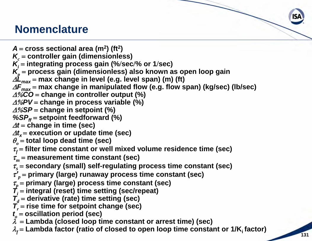
131

A = cross sectional area (m2) (ft2) Kc = controller gain (dimensionless) Ki = integrating process gain (%/sec/% or 1/sec) Kp = process gain (dimensionless) also known as open loop gain ∆Lmax = max change in level (e.g. level span) (m) (ft) ∆Fmax = max change in manipulated flow (e.g. flow span) (kg/sec) (lb/sec) ∆%CO = change in controller output (%) ∆%PV = change in process variable (%) ∆%SP = change in setpoint (%) %SPff = setpoint feedforward (%) ∆t = change in time (sec) ∆tx = execution or update time (sec) θo = total loop dead time (sec) τf = filter time constant or well mixed volume residence time (sec) τm = measurement time constant (sec) τs = secondary (small) self-regulating process time constant (sec) τ’p = primary (large) runaway process time constant (sec) τp = primary (large) process time constant (sec) Ti = integral (reset) time setting (sec/repeat) Td = derivative (rate) time setting (sec) Tr = rise time for setpoint change (sec) to = oscillation period (sec) λ = Lambda (closed loop time constant or arrest time) (sec) λf = Lambda factor (ratio of closed to open loop time constant or 1/Ki factor)

Nomenclature

132

Ei = integrated error for unmeasured load disturbance (% sec) Ex = peak error for unmeasured load disturbance (%) Eo = open loop error (loop in manual) for unmeasured load disturbance (%) Ki = near integrator process gain (% per % per sec) Ko = open loop gain (dimensionless product of valve, process, and measurement gains) Kx = detuning factor for controller gain (dimensionless) Nm = measurement noise (%) ∆%CO/∆t = rate of change in PID % controller output (% per sec) ∆%PV/∆t = rate of change in PID % process variable (% per sec) ∆Tw = wireless default update rate (update time interval) (sec) Sm = wireless measurement trigger level (threshold sensitivity) (%) Sv = valve stick-slip, resolution, or deadband (%) T63 = 63% process response time (sec) θo = original loop dead time (sec) θ∆t = additional dead time from default update rate (sec) θs = additional dead time from wireless trigger level (sec) θv = additional dead time from valve (sec) θw = additional dead time from wireless measurement (sec) ρ = fluid density (kg/m3) (lb/ft3) τo = self-regulating open loop time constant (largest time constant in loop) (sec) τ’o = runaway open loop time constant (positive feedback process time constant) (sec)

Nomenclature