frequency response methods - amirkabir university of...
TRANSCRIPT

FrequencyResponse Methods
Ktion 302
....-Of Response Plots 304Example of Drawing the Bode Diagram 321
~"'IIQ Response Measurements 325
!'d"owoce Specifications in the Frequency Domain 327
Mapitude and Phase Diagrams 330
Example 332
335
examined the use of tcst input signals such as a step and a ramp sig1IdI chapter, we will use a steady-state sinusoidal input signal and con
response of the system as the frequency ofthc sinusoid is varied. Thus~ at the response of the system to a changing frequency, w.Will examine the response of G(s) when s = jw and develop several
ot:~ttin8 the complex number for GUw) when w is varied. These plOlSUlSighl regarding the performance of a system. We are able to develop
Performance measures for the frequency response of a system. The mea:0 be used as system specifications and we can adjust parameters inmeet the specifications.
301
We will consider the graphical development of one or more form r.frequency response plot. We can then proceed to use computer-gener:t ~r thtto readily obtain these plots, e data
302 Chapter 7 Frequency Response Methods
III Introduction
In the preceding chapters the response and performance of a system haydescribed in terms of the complex frequency variable s and the locatione~poles and zeros on the s·plane. A very practical and important alte~ .approach to the analysis and design of a system is the frequency response met':The freqllenc~ res~ons~ ofa ~ys,em is de.(ined .Qs./he sr~ady-state reSponse old.,system to a smusOidai mput sIgnal. The SinUSOid IS a umque input signal, and theresulting output signal for a linear system, as well as signals throughout the SySO
tern, is sinusoidal in the steady state; it differs from the input wavefonn only illamplitude and phase angle.
One advantage of the frequency response method is the ready availability ofsinusoid test signals for various ranges of frequencies and amplitudes. Thus theexperimental determination of the frequency response of a system is easityaccomplished and is the most reliable and uncomplicated method for the exper-.imental analysis ofa system. Often, as we shall find in Section 7.4, the unknowatransfer function ofa system can be deduced from the experimentally determinedfrequency response ofa system [1,2]. Furthermore, the design ofa system in thefrequency domain provides the designer with control of the bandwidth of a system and some measure of the response of the system to undesired noise aDddisturbances.
A second advantage of the frequency response method is that the transferfunction describing the sinusoidal steady-state behavior of a system can beobtained by replacing s with jw in the system transfer function T(s). The transferfunction representing the sinusoidal steady-state behavior of a ~ystem .is the~function of the complex variable jw and is itself a complex functIOn TUw) wb. )possesses a magnitude and phase angle. The magnitude and phase angle of n::,are readily represented by graphical plots that provide a significant insight foranalysis and design of control systems. . aad
The basic disadvantage of the frequency response met~od for an~IYS~rectdesign is the indirect link between the frequency and the ttme do~aln~nsieDIcorrelations between the frequency response and the correspondlOg t 0C1response characteristics are somewhat tenuous, and in p~cti~e th~ f~I~~~response characteristic is adjusted by using various design cntena which WI
mally result in a satisfactory transient response. .The Laplace transform pair was given in Section 2.4 and is written as.
F(s) - LUll») = J.m j(t)e-' dl

r: 1J(t) I dl < 00.
303
(7.6)
(7.5)
(7.4)
(7.3)
(7.2)
7.1 Introduction
CUw) • TU· )RU· _ G(jw) .w w) - 1 + GUw)HUw) RUw).
1 J,'j.J(I) - r'IF(s)} ~ -. F(s)e" ds,
21fJ ._joe>
complex variable s = u + jw. Similarly, Ihe Fourier transform pair is
';UIPut .fre~uency response of a single-loop control system can be). SUbstltutmg s = jw in the closed-loop system relationship, C(s) =
10 that we have
Fourier and Laplace transforms are closely related, as we can see byEqs. (7.1) and (7.3). When the function f(t) is defined only for t > 0,the case, the lower limits on the integrals are the same. Then, we note
two equations differ only in the complex variable. Thus, if the Laplaceofa function;;(t) is known to be Fj(s), we can obtain the Fourier trans
1his same time function F,Uw) by setting s = jw in F,(s).we might ask, because the Fourier and Laplace transforms are so
, why not always use the Laplace transform? Why use the Fourierat all? The Laplace transform permits us to investigate the s-plane loca
lite poles and zeros of a transfer T(s) as in Chapter 6. However, the freIIIpOnse method allows us to consider the transfer function T(jw) andourselves with the amplitude and phase characteristics of the system.
to investigate and represent the character of a system by amplitudeequations and curves is an advantage for the analysis and design of
s.•consider the frequency response of the closed-loop system, we mightlDpUt r(l) that has a Fourier transform, in the frequency domain, as
(7.7)
Chapter 7 F~ue.ncy Response: Methods304
Utilizing the inverse Fourier transform, the output transient response wQuid be
e(1) = :7-'{C(jw)} - 2~ L: C(jw)ei'" dw.
However, it is usually quite difficult to evaluate this inverse transform ifor any but the simplest systems, and a graphical integration may be Usedn~~natively, as we wiJl nOlc in sUcceeding sections, several measures of the l~n .Iet.response can be related to the frequency characteristics and utilized for d~~pu~s. P
_ Frequency Response Plots
The transfer function ofa system G(s) can be described in the frequency dOrnailby the relationt
GUw) = G(,)! .... - RUw) + jXUw), (7.1)
where
RUw) - Re[GUw))
and
XUw) - Im(GUw)).
Alternatively, the transfer function can be represented by a magnitude IG U,,)Iand a phase tM,jw) as
GUw) = IG(jw)!e""'" = IG(w)!~, (7.9)
where
¢(w) = tan-I X(w){R{w)
and
IG(w)I' - (R(w)]' + [X(w)]'.
GU ) ...The graphical representation of the frequency response of t~e system Ii ~utilize either Eq. (7.S) or Eq. (7.9). The polar plol representatIOn oflhe
lreQ
redie
response is obtained by using Eq. (7.S). The coordinates of the polar p 0; a po/JJIreal and imaginary parts of GUw} as shown in Fig. 7.1. An e~amplc 0 apial will illustrale Ihis approach.
tSee Appcndi,l E for a review oroomplc,l numb<'r1.

R+ +
305
(7.11)
(7.10)
(7.12)
1=}~(;-w7/w-',);-+"---;1 •
Im(G) - X(o;.J)
7.2 Frequency Re,ponse Plots
Figure 7.1. The polar plane.
------t..,--- Re(C) - R(o;.J)
GUw) = IG(w)IU&!. (7.13)
Vlo~_) CL(I)Figure 7.2. An RC filter.
WI = lIRe.polar plot is obtained from the relation
GUw) = R(w) + }X(w)
_ ,1_-7""}"(w,,/:,,w'C,)(wlwl)2 + I
_,Ie 7.J Frequency response of an RC filter
Refilter is shown in Fig. 7.2. The transfer function of this filter is
Vl(s) IG(s) ~ V,(s) - Res + I •
j(wlwl)= 71-+'-;-(W"C/-w ,")1 I + (wlwl)l .
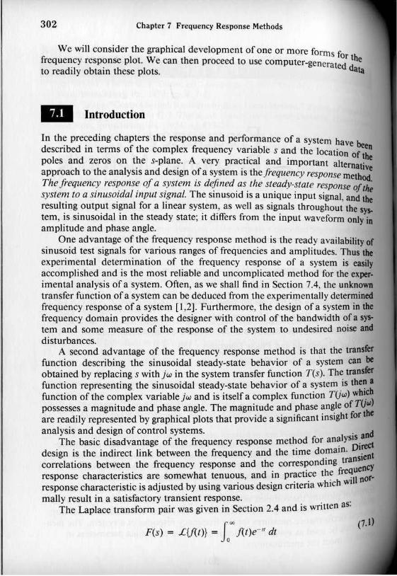
oftbe rea.I and imaginary pans is shown in Fig. 7.3 and is easily shownwith the center at (~ 0). When w = W1l the real and imaginary pans
aDd the angle cP(w) = 45-. The polar plot can also be readily obtained(7.9) ..
liDusoidal sleady-state transfer function is
306
where
Chapter 7 Frequency Response Methods
X(w)
___ N~&illi"" W
//... -....,"", ,\I \
=W-=--;--=-,*_-._~__\l-',-'~_""_+_ ,.,=0 lI(w)4S· -
'GI
~ w=w[!'wI;..., ....
figure 7.3. Polar plot for RC filler.
IIG(w)j "" [I + (wlw,r]ln and 41Cw) = -lan~l(wlw,).
Clearly, when w = w., magnitude is IG(wl)1 = 1/V2 and phase 4>(w.) "" -45".AJso, when w approaches +00, we have IG(w)l -- 0 and I/>(w) = -90-. Similatty.when (oj = 0, we have I G(w) I = I and I/I(w) = O.
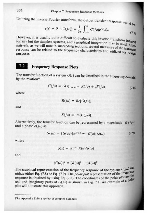
• E x amp Ie 7.2 Polar plot of a transfer function
The polar plot of a transfer function will be useful for investigating system ..bility and will be utilized in Chapter 8. Therefore it is wonhwhilc 10 compldeanother example at this point. Consider a transfer function
G GK K (7.14)
I (s)I$_j. -= Uw) = jw(jWT + 1) = jw _ WIT·
Then the magnitude and phase angle are written as
(7.111
and
.;(w) = -tan-' (_~). "
The phase angle and the magnitude are readily calculated at th~ freq.ue~~l~~1.1.0, w = liT, and w - +00. The values of IG(w)l and cP(w) are gIVen mand the polar plot of GUw) is shown in Fig. 7.4.

307
(7.16)
(7.17)
o00
-ISO"
7.2 )o'requency Response Plots
ImlG)
_____w"'-'-~-*_ _.,_k~JGI
PO$ili~ w
Fiaure 7.4. Polar plol for GUw} - K/jw(jr..n- + I).
T.bk 7.1.
"0 '" 11'
1(;<-)1 ~ 4K'IVS K'/V2
~") -90" -llr -135"
GUw) = IG(w) Ie i • l ..J•
Ioprithm ofEq. (7.16) is
In GUw) ~ In IG(w)1 + j¢{w),
II'e several possibilities for coordinates of a graph portraying the frc-
:
:::ofa system. As we have seen, we may choose to utilize a polart the frequency response (Eq. 7.8) ofa system. However, the lim
polar plots are readily apparent. The addition of poles or zeros to an."..." requires the recalculation of the frequency response as outlined
7.1 and 7.2. (See Table 7.1.) Furthermore, the calculation of the fresc in this manner is tedious and does not indicate the effect of the
poles or zeros.the introduction of logarithmic plots, often called Bode plots, sim
determination of the graphical portrayal of the frequency response. Theplots are called Bode plots in honor of H. W. Bode, who used themin his studies of feedback amplificrs [4,5]. The transfcr function in the
domain is

308 Chapter 7 Frequency Response Methods
0r-"'O:::::::::---------_
+
-++--IO~
,.I'=---------~(~.)'------------
-90"
° I ( , , ,-
" ," , "w
("
Figure 7.5. Bode diagram for GUw) '" IIUwr + I).
where In IG I is the magnitude in nepers. The logarithm of the magnitude is normally expressed in terms of the logarithm to the base 10, so that we use
Logarithmic gain = 20Iog,o IG(w)l.
where the units are decibels (db). A decibel conversion table is given in APpendiJD. The logarithmic gain in db and the angle .p(w) can be plotted versus the fiequency w by utilizing several different arrangements. For a Bode diagram, the pIoIof logarithmic gain in db versus Col is normally plotted on one set of axes. and::phase «w) versus Col on another set of axes. as shown in Fig. 7.5. For exam.ple,Bode diagram of the transfer function of Example 7.1 can be readily obtained. IIwe will find in the following example.
• E x amp Ie 7.3 Bode diagram of an RC filler
The transfer function of Example 7.1 is
GUw) = jw{R~ +_ --,1_
jwr + I'
(7.181
Figure 7.6. Asymptotic. curve for UWT + I)-I.
(7.21 )
309
(7.22)
(7.20)
(7.19)
,,-20~,--.L-~,-_L_-,,!,0
10,
7.2 frequency Relponse Plots
20 log IGI - -10 log 2 - -3.01 db.
·tude plot for this network is shown in Fig. 7.5(a). The phase angle ofis
""i -101--+--t-~l-.---1?,
l' = Re,
stant of the network. The logarithmic gain is
- 'n20 log IGI ~ 20 lOge +1<=),) - -10 log(1 + (wd').
fi:equencies, that is III « 1/1', the logarithmic gain is
20 log IGI = -10 log (I) - 0 db, w « I/T.
tequencies, that is Ill» 1/1', the logarithmic gain is
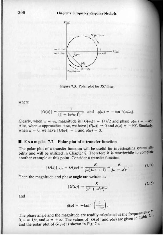
20 log IGI = -2010gWT W» 1/1',
20 log IGI = -20 log = _ -20 log T - 20logw. (7.23)
a set of axes where the horizontal axis is log w, the asymptotic curve for~ a straight line, as shown in Fig. 7.6. The slope of the straight line can
'-.dfrom Eq. (7.21). An interval of two frequencies with a ratio equal
plot is shown in Fig. 7.5(b). The frequency w = 1/1' is often called the~:::;: or corner frequency.• the Bode diagram of Fig. 7.5, we find that a linear scale of fre·it Dollhe most convenient or judicious choice and we should consider
aloprilhmic scale offrequency. The convenience ofa logarithmic scalecan be seen by considering Eq. (7.21) for large frequencies w» 1/1',
Chapter 7 Frequency Response Methods
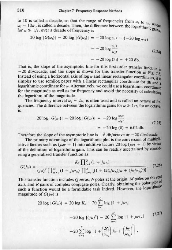
to 10 is called a decade, so that the range of frequencies from w to(,)2 = lOw" is called a decade. Then, the difference between the logalrith;i~w~for w» I/T, over a decade of frequency is &alns.
20 log IG(wl)1 - 20 log IG(W2) I = -20 log WIT - (-201og W;lT)
310
w,'= -20 log-w" (7.24)
- -20 Jog (X.) - +20 db.
That is, the slope of the asymptotic line for this first-order transfer functi .-20 db/decade, and the slope is shown for this transfer function in Fig.°~:Instead of using a horizontal axis of log wand linear rectangular coordinates, i;·simpler to use semilog paper with a linear rectangular coordinate for db and ..logarithmic coordinate for w. Alternatively, we could use a logarithmic coordirw:for the magnitude as well as for frequency and avoid the necessity of calculatioathe logarithm of the magnitude.
The frequency interval Wl = 2w, is often used and is called an octave of fie.quencies. The difference between the logarithmic gains for w» lIT, for an octave,is
20 Jog IG(w,) I - 20 Jog IG(w,) I w""" -2010g-WZT (7.25)
= - 20 Jog (~) = 6.02 db.
Therefore the slope of the asymptotic line is -6 db/octave or - 20 db/dt:(:adc.The primary advantage of the logarithmic plot is the conversion ofmultipti.
cative factors such as (jWT + I) into additive factors 20 log UWT + I) by virtueof the definition of logarithmic gain. This can be readily ascertained by considering a generalized transfer function as
Kb Il~., (l + jWT;)GU ) (7.26)
w = UW!, IT:., (J + i-m) IT;., [(I + (2'.Iw,,liw + Uwjw,,)')(
This transfer function includes Qzeros, N poles at the origin, M poles on the~axis, and R pairs of complex conjugate poles. Clearly, obtaining the polar ~~t itsuch a function would be a formidable task indeed. However, the logant mmagnitude of G(jw) is
Q
20 log IG(w)1 = 20 Jog K. + 20 L: Jog II + i-,I,. ,"-20 Jog IUwtl - 20 L: Jog I J + iw,,, I
(7.21)
m·'

311
(7.30)
(7.28)
A pole at the origin has a logarithmic
7.2 Frequency Response Plots
Q M
+ L tan-I W'Tj - N(900) - L tan-I W'T",
i_I m_1.p(w)=
The logarithmic gain is
20 log Kh = constant in db,
angle is zero. The gain curve is simply a horizontal line on the Bode
tpin Kb
(or zeros) at the origin (jw)
or zeros on the real axis (jW'T + I)
x conjugate poles (or zeros) [I + (2r/w~)jw + (jw/w-f]
limply the summation of the phase angles due to each individual factorfunction.the four different kinds offactors that may occur in a transfer func-
• follows:
determine the logarithmic magnitude plot and phase angle for these fourthen utilize them to obtain a Bode diagram for any general form of a
function. Typically, the curves for each factor are obtained and thenr graphically to obtain the curves for the complete transfer function.
• this procedure can be simplified by using the asymptotic approxi!O these curves and obtaining the actual curves only at specific imponant
Bode diagram can be obtained by adding the plot due to each individualnnore, the separate phase angle plot is obtained as
20 log L~I = -20 log w db (7.29)
~rangle 4{~) ~ -90·, The s.lope of the magnitude curve is -20a pole, SImilarly for a multiple pole at the origin, we have
20 log IU~)"ll = -20Nlogw,

901-----1----+---1li"')
r---,---,--,Ii"'):'80
li",I-:-llloL__-L_--f.;---~""
0.1 10
~• ol-----I------j---1 (/lJ{)
3'Q --9
01-- I--__--j 1fi"'I-
1
Chapter 7 Frequency Response Methods
(/",1-'
-'0'C----!-'---'~-~0.1 10 100
w
Ii"')
,,"'--,-----,,-----:71
"' 0 f-----=;iIC '---+----1
Figure 7.7. Bode diagram forUw)iN.
312
Poles or Zeros on the Rea! Axis. The pole factor (I + jWT)-1 has been coa.sidered previously and we found that
20 log I, +'jwTI = -10 log (1 + w2r
2). (7.32)
The asympl~tjccurve for w <~ liT is 20 log I = 0 db, and the asymptotic curvefor w» lIT IS - 20 log WT whIch has a slope of - 20 db/decade. The intcrsectiolof the two asymptotes occurs when
20 log 1= Ddb = -2010gwT
or when w = 1fT, the break frequency. The actual logarithmic gain when I.Al •
l/r is - 3 db for this factor. The phase angle is 1>(w) = -tan-I W1" for the denominator factor. The Bode diagram of a pole factor (I + jwr)-J is shown in Fig. 7.S.
The Bode diagram of a zero factor (l + jW1") is obtained in the same manneras that of the pole. However, the slope is positive at +20 db/decade, and thephase angle is <p(w) = +tan- I
WL
A linear approximation to the phase angle curve can be obtained as shown illFig. 7.8. This linear approximation, which passes through the correct phase at tilebreak frequency, is within 6° of the actual phase curve for all frequencies. TbiIapproximation will provide a useful means for readily determining the form ofthe phase angle curves of a transfer function G(s). However, often the accuratephase angle curves are required and the actual phase curve for the 6rst-order~tor must be drawn. Therefore it is often worthwhile to prepare a cardboard }:plastic) template which can be utilized repeatedly to draw the phase curves
and the phase is cP(w) = -90°N. In this case the slope due to the multi I- 20N db/decade. For a zero at the origin, we have a logarithmic mag p. e Polt ..
nllUl!t20 log IJwl = +20 log w,
. Q-Iwhere the slope IS +20 db/decade and the phase angle is +90·, The Bod d'of the magnitude and phase angle OfUW):tN is shown in Fig. 7.7 for N
C:=l~
N-2. ~

,LO
313
Asymptoticcurvr-------
,w
(.)
Enctcurvr
7.2 Frequency Response Plots
(b)
Figure 7.8. Bode diagram for (1 + jWTr l.
Linrarappro"imatioR
Conjugate Poles or Zeros [I + (2r/w~)jw + (jwlw~Y]. The qua·for a pair of complex conjugate poles can be written in normalized
"
[I + j2ru - u2r l, (7.33)
0.10 0.50 0.76 1.31 2 5 )0
-0.04 -1.0 -2.0 -3.0 -4.3 -7.0 -14.2 -20.04
0 0 0 0 -2.3 -6.0 -14.0 -20.0-5.7 -26.6 -37.4 -45.0 -52.7 -63.4 -78.7 -84.3
0 -31.5 -39.5 -45.0 -50.3 -58.5 -76.5 -90.0
ual factors. The exact values of the frequency response for the pole)-1 as well as the values obtained by using the approximation for com
areaiven in Table 7.2.

and the phase angle is
where u = wlw~. Then, the logarithmic magnitude is
20 log IG(w)l - -10 log ((I - u')' + 4I'u'),
Chapter 7 Frequency Response fotethods314
¢(w) -(7.lll
When 11 « I, the magnitude is
db - -IOlog I ~ Odb,
and the phase angle approaches 0°, When Ii » I, the logarithmic magnitudeapproaches
db = - Ia log It = ~40 log u,
which results in a curve with a slope of -40 db/decade. The phase angle, wbeau » I, approaches - 180°. The magnitude asymptotes meet at the O-db line wheau = w/w~ = 1. However, the difference between the actual magnitude curve IDdthe asymptotic approximation is a function of the damping ratio and must beaccounted for when t < 0.707. The Bode diagram of a quadratic factor due to.pair of complex conjugate poles is shown in Fig. 7.9. The maximum value oflbefrequency response, Mp~, occurs at the resonanl freqllency w,. When the dampiDaratio approaches zero, then w, approaches W q , the natural frequency. The resonaDIfrequency is determined by taking the derivative of the magnitude of Eq. (7.33)with respect to the normalized frequency, II, and setting it equal to zero. The raonant frequency is represented by the relation
and the maximum value of the magnitude IG(w) I is
AI,. _ IG(w,) I - (2,,/1-=1')-', ,< 0.707, (7.31)
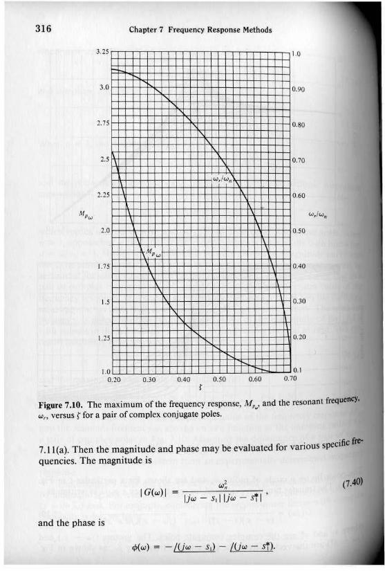
for a pair of complex poles. The maximum value of the frequency :espon~ Me:and the resonant frequency w, are shown as a function of the damping .ratlO~a pair of complex poles in Fig. 7.10. Assuming the dominance of a pair of'mllplex conjugate closed-loop poles, we lind that these curves are use~ul for es~iog the damping ratio of a system from an experimentally detenmned freqresponse. plJJlt
The frequency response curves can be evaluate~ graphically .on th:I~~g tbCby determining the vector lengths and angles at vanous frequencles.(I) (11p1e1(5 = +jw).axis. For example, considering the sccond-order faclor WIth CO
conjugate poles, we have
(7.36),< 0.707,21',• W = W Vi, .
1 w;G(5) = 'C(s-"/w-."')"+-,--'2'"',-"s/C'w-.-"+--"j = s! + 2fw..s + w; .

315
J 4 5 6 8 10,(oJ
u _ fJlw~ • fr~Qu..nc)' ratio
7.2 Frequency RelponSf: Plotl
0.3 0.4 0.5 0.6 0.8 1.00.2
0.2 0.) 0.4 O.S 0.6 0.8 1.0
W/IJ. - Frcqucncy ratio
(b)
JIpn 1.9. Bode diagram for GUw) :::: [I + (2t/w.)jw + Uwlw.)Zl~l.
lie on a circle of radius w. and are shown for a particular r in Fig.The transfer function evaluated for real frequency s = jw is written as
G(jw) ~ w; I ~. w;. , (7.39)(s SIXS sTl .-jo. Uw - slXlw - s!)
I. IDd sT are the complex conjugate poles. The vectors Uw 5,) andIre the vectors from the poles to the frequency jw. as shown in Fig.
--+-0.3 ~§i§'-- t-_-+O._
40.5
r 0.6
D',",""--t--t-+--F l.0
316 Chapter 7 Frequency Response Methods
3.25 1.0
3.0 0.90
2.75 0.80
2.5 0.70
w,/<.Jn
2.2S 0.60
Mp,,", w,lw.
2.0 0.50
/of,..,1,75 DAD
1.5 0.30
1.25
1.00.20 0.30 0.40 o.so 0.60
0.20
0.10.10,
Figure 7.10. The maximum of the frequency response, M" and the resonant frequencY.w" versus t for a pair of complex conjugate poles. ~
7.II(a). Then the magnitude and phase may be evaluated for various specific~quencies. The magnitude is
and the phase is
w;IG(w) I = .,,----=,.-----=0
Ij", - 51! IJ'" - sf I '
iP(w) = -IU.., - 5,) - IV", - si)·
(7.40)

in Fig. 7.1 t in parts (b), (c), and (d), respectively. The magnitude andoding to lhese frequencies are shown in Fig. 7.12.
317
o
(7.4\)
(b)
Cd)
I I ;w~
#t~r-"':f-
,f.!I
0
I ~
I1-\\81
I,
I'>i
II 0I, 1-
.IA,.I
w = w"
7.2 Frequency Response Plots
w = 0,
w ,
(.)
(0)
FIgure 7.11. Vector evaluation of the frequency response.
IPlilUcle and phase may be evaluated for three specific frequencies:
1-+-+-1'. ,"'" r-
Bode diagram of twin-T network
elamplc of the delennination oflhe frequency response using the pole.zeroand the Vectors tojw, consider the twin·T network shown in Fig. 7.13transfer function of this network is
G E".is) (sr)2 + 1(5) = Ein(s) = (sr)2 + 4ST + I '

Chapler 7 Frequenc)' Response Methods318
M -'w
1.0
05
00o w,
w
"w)
- <1'
.....
-180"
Figure 7.12. Bode diagram for complex conjugate poles.
Figure 7.13. Twin-T network.
where T = RC. The zeros are at ±jl and the poles are at -2 ± V3 in the Sf'
plane as shown in Fig. 7.14(a). Clearly, at w = 0, we have IGI = I and¢{w)0°. At w = l/r, IG I = 0 and the phase angle of the ve{;tor from the zero at Sf •
jl passes through a transition of 180". When w approaches 00, IG I = I and4>(w) = 0 again. Evaluating several intermediate frequencies, we can readilyobtain the frequency response, as shown in Fig. 7.14(b).
In the previous examples the poles and zeros of G(s) have been restricted 10the left.hand plane. However, a system may have zeros located in the right-hands-plane and may still be stable. Transfer functions with zeros in the right.hand~plane are classified as nonminimum phase-shift transfer functions. If the zeros ofa transfer function are all reflected about the jw~axis, there is no change in ~magnitude of the transfer function, and the only difference is in the phase..shiftcharacteristics. If the phase characteristics of the two system functions are co~pared, it can be readily shown that the net phase shift over the frequency rantefrom zero to infinity is less for the system with all its zeros in the left-hand ~

319
(b)
'I,
T--
T~, I I
I,
.: 91I~~i t-
oTI_l_~ 1__________L_
'~Tjm~fV~~mvto
o
90"
-90
~~l<' ".;
" I G,oj I0 .,
7.2 Frequency Response Plots
"~ 0
(.)
7.14. Twin-T network. (a) Pole-zero pattern. (b) Frequency response.
w W'7.15. Polc-ze . . ._",,'.. ro patterns gIVing the same amplitude response and different phase
Thus the transfer function GI(s), with all its zeros in the left-hand s-plane,a minimum phase transfer function. The transfer function G2(s), with
~I - IGIUw)1 and all the zeros ofG\(s) reflected about thejw-axis into thes-plane, is called a nonminimum phase transfer function. Reflection
mo or pair of zeros into the right-half plane results in a nonminimumtransfer function.
two pole-zero patterns shown in Fig. 7.15(a) and (b) have the samecharacteristics as can be deduced from the vector lengths. However,characteristics are different for Fig. 7.15(a) and (b). The minimum
do"'_ristic of Fig. 7. I5(a) and the nonminimum phase characteristic of5(b)are shown in Fig. 7.16. Clearly, the phase shift of
G\(s) = s + zs+p

320 Chapler 7 Frequency Response Methods
180·
NonTIlinimllm phzo,
Minimum
"".~
o,L..",""''----",------:p--=
Figure 7.16. The phase characteristics for the minimum pha2 and nonminimum phase:transfer function.
ranges over less than 80·, whereas the phase shift ofs - ,
Gb)~--s+p
ranges over 180·, The meaning of the term minimum phase is illustrated by F..7.16. The range of phase shift ora minimum phase transfer function is the~
c.) (b)
~, ~"'"
1-t Illi\
-~-Trl ------------+0 v./..;- 0+
~ti~ tout
0 0
-360' w. w-",FllllTe 7.17. The all-pass network pole-zero pattern and frequency respOnse.

An Example of Drawing the Bode Diagram
321
(7.42)
7.3 An Example of Drawing the Bode Diagram
we plOl the magnitude characteristic for each individual pole and zerothe constant gain.
ot gain K = 5at the originat w = 2at w = 10
ofcomplex poles at w = w. = 50
GUw) = 5(1 + jD.lw)jw(l + jO.5w)(1 + jO.6(wj50) + Uwj50)')·
n, in order of their occurrence as frequency increases, are as follows:
diagram of a transfer function G(s), which contains several zeros andII obtained by adding the plot due to each individual pole and zero. The"ty ofthis method will be illustrated by considering a transfer function that
all the factors considered in the preceding section. The transfer functionis
I
or minimum corresponding to a given amplitude curve, whereas theof the nonminimum phase curve is greater than the minimum possible for
amplitude curve.particularly interesting nonminimum phase network is the all~pass net_cb can be realized with a symmetrical lattice network (B]. A symmet
of poles and zeros is obtained as shown in Fig. 7.17(a). Again, theIG I remains constant; in this case, it is equal to unity. However, the
from 0° to -360°. Because 9l = 180° - 91 and 9! = IBO° - 91,ilgiven by ¢(w) = -2(8) + (1). The magnitude and phase characteristic
.....pass network is shown in Fig. 7.17(b). A nonminimum phase latticeilshown in Fig. 7. I7(c).
COnstant gain is 20 log 5 = 14 db, as shown in Fig. 7.IB.
~itude of the pole at the origin extends from zero frequency to infinitelIenCICS and has a slope of ~ 20 db/decade intersecting the O-db line at
- I, as shown in Fig. 7.IB.
8S)'mptotic approximation of the magnitude of the pote at w = 2 has a?f - 20 db/decade beyond the break frequency at w = 2. The asymptotictUde below the break frequency is 0 db, as shown in Fig. 7.18.
asymptotic magnitude for the zero at w = + 10 has a slope of +20beyond the break frequency at w = la, as shown in Fig. 7.18.

322 Chapter 7 Frequency Response Methods
Therefore the total asymptotic magnitude can be ploned by adding theasymptotes due to each factor, as shown by the solid line in Fig. 7.19. Examininathe asymptotic curve of Fig. 7.19, onc notes that the curve can be obtained
SO 100
10
w
Figure 7.19. Magnitude characteristic.
0
~20 Jblde~0 ,
'~0
,-40 db/dec
0
Vuel CU"'j0
Approximate CU"'~~~~~~ee0
-60dE10
I0 11)0-s
0.1
-,
°l~ CD,'"0
@
/ ~0
~ "-~
'",
0
0 ~0.1 0.2 1 2 10
-I
2
-2
Figure 7.18. Magnitude asymplOles of poles and zeros used in the example.
-I
-2
2
-3
5. The asymptotic approximation for the pair of complex poles at w = W n = 50has a slope of -40 db/decade due to the quadratic forms. The break frequencyis w = w~ = 50, as shown in Fig. 7.18. This approximation must be correctedto the actual magnitude because the damping ratio is r = 0.3 and the magni·tude differs appreciably from the approximation, as shown in Fig. 7.19.
323
60 '00
Compln pole5
Zerou..,-IO
Approltimate «..,j
"
Pole at origin
Pole at "" = 2
2.01.0
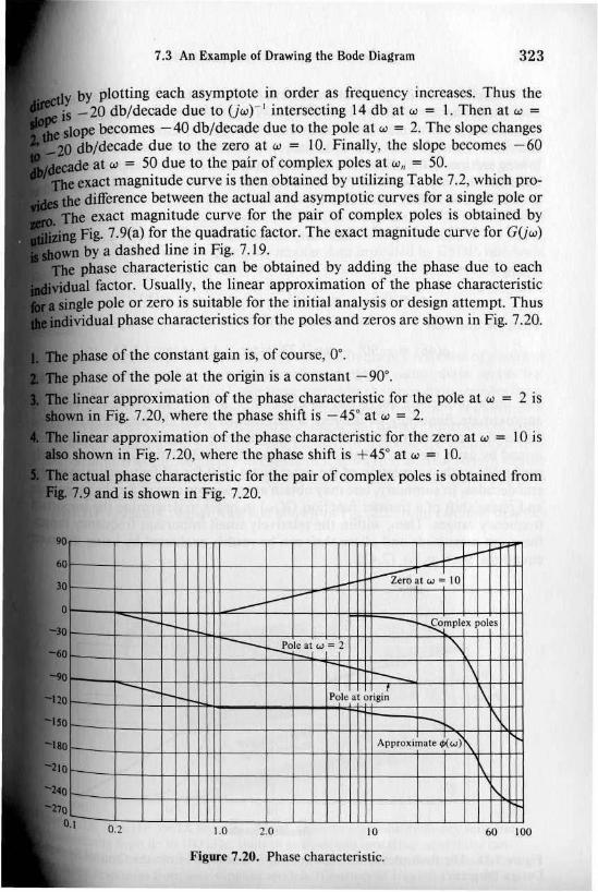
Figure 7.20. Phase characteristic.
7.3 An Example of Drawing the Bode Diagram
0.2
phase of the constant gain is, of course, 0°.phase of the pole at the origin is a constant -90°.linear approximation of the phase characteristic for the pole at w = 2 is
in Fig. 7.20, where the phase shift is -45° at w = 2.linear approximation of the phase characteristic for the zero al w = lOisshown in Fig. 7.20, where the phase shift is +45° at w = 10.actual phase characteristic for the pair of complex poles is obtained from7.9 and is shown in Fig. 7.20.
by plotting each asymptote in order as frequency increases. Thus the-20 db/decade due to (jW)-1 intersecting 14 db at w = I. Then at w =pc becomes -40 db/decade due to the pole at w = 2. The slope changes
db/decade due to the zero at w = 10. Finally, the slope becomes -60at w = 50 due to the pair of complex poles at Wn = 50.
exact magnitude curve is then obtained by utilizing Table 7.2, which prodifference between the actual and asymptotic curves for a single pole orexact magnitude curve for the pair of complex poles is obtained by
Fig. 7.9(a) for the quadratic factor. The exact magnitude curve for GUw)by a dashed line in Fig. 7.19.phase characteristic can be obtained by adding the phase due to each
factor. Usual1y, the linear approximation of the phase characteristice pole or zero is suitable for the initial analysis or design attempt. Thus
'vidual phase characteristics for the poles and zeros arc shown in Fig. 7.20.

324 Ch~pter 7 Frequency Ruponse Methods
Therefore the total phase characteristic, 4>«(0), is obtained by adding thdue to each factor as shown in Fig. 7.20. While this curve is an approxi~P~its usefulness merits consideration as a first attempt to determine the phaseall0n,
acteristic. Thus, for example, a frequency of interest, as we shall note in thc~.Jowing section, is that frequency for which tP(w) ""' -180·. The approximate e 01indicates that a phase shirt of -180- occurs at w s: 46. The actual phases~w ., 46 can be readily calculated as I II
4>(w) = -90· - 130-1 WTl + 130-1 WT~ - tan- l I 2ru l'- u (7.43)
where
Tl = 0.5. Tl = 0.1, Ii = w/w~ = w/50.
Then we find that
¢(46) = -90· - tan- l 23 + 130-1 4.6 - 130- 1 3.55
= -175·, (7.44)
and the approximate curve has an error of 5° at w = 46. However, once theapproximate frequency of interest is ascertained from the approximate phalecurve, the accurate phase shift for the neighboring frequencies is readily determined by using the exact phase shift relation (Eq. 7.43). This approach is usualtypreferable to the calculation of the exact pbase shift for all frequencies over sev~
eral decades. In summary, one may obtain approximate curves for the magnitudeand phase shift of a transfer function GUw) in order to determine the importaldfrequency ranges. Then, within the relatively small important frequency raJ1Fl,the exact magnitude and phase shift can be readily evaluated by using. the exactequations, such as Eq. (7.43).
Max. mag • JJ.96906dBMax. phalot - -92.J58U lit.~g;Jjnis2500
""n.mag __ 112.0l3IdlJM1n.~- -268.7353l1tg
-----,
Mag:,Phase:
\\\ ,
'-'" HII I."
OdB
.1
dB"d
Pha!oC
Fmjuency. radi_
I SySICIllfiaure 1.21. The Bode plot of the GUw) ofEq. 7.42 obtained from Ihe ContrODesian Program.
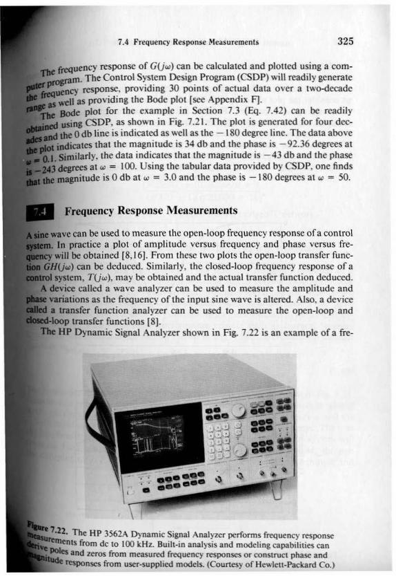
Frequency Response Measurements
3257.4 Frequency Response j\1easurements
7.12. The HP 3562A Dynamic Signal Analyzer performs frequency responsets from de to 100 kHz. Built-in analysis and modeling capabilities can
JoIics and zeros from measured frequency responses or construct phase and~nses from user-supplied models. (Counesy of Hewlelt-Packard Co.)
wave can be used to measure the open-loop frequency response ofa controlIn practice a plot of amplitude versus frequency and phase versus fre
will be obtained [8,16). From these two plots the open-loop transfer funcU"') can be deduccd. Similarly, the closed-loop frequency response ofa
system, TUw). may be obtained and the actual transfer function deduced.device called a wave analyzer can be used to measure the amplitude andvariations as the frequency of the input sine wave is altered. Also, a device• transfer function analyzer can be used to measure the open-loop and
transfer functions 18).HP Dynamic Signal Analyzer shown in Fig. 7.22 is an example ofa fre-
fi"eQuency rcsponse of GUw) can be calculated and plottcd using a comm. Thc Control System Design Program (CSDP) will readily generate
......"" response. providing 30 points of actual data over a two-decade.11 as providing the Bode plot (see Appendix Fl.Bode plot for the example in Section 7.3 (Eq. 7.42) can be readilyusing CSDP, as shown in Fig. 7.21. The plot is generated for four decabe 0 db line is indicated as well as the -180 degree line. The data above
jadicatcS that the magnitude is 34 db and the phase is -92.36 degrees at•Similarly. the data indicates that the magnitude is -43 db and the phasecIe&J'eCS at w = 100. Using the tabular data provided by CSDP, one findslDIIJlitude is 0 db at w = 3.0 and the phase is -180 degrees at w = 50.

quency response measurement tool. This device can also synthesize the frcqUresponse ofa model ofa system allowing a comparison with an actual rcsPQcney
As an example of determining the transfer function from the BOde PlaInS(.us consider the plot shown in Fig. 7.23. The system is a stable circuit consis~.leIof resistors and capacitors. Because the phase and magnitude decline a In,increases between to and 1000, and because the phase is _45 0 and the gain ~~db at 370 fad/sec, we can deduce that one factor is a pole near w = 370. BeYOnd370 fad/sec, the magnitude drops sharply at ~40 db/decade, indicating thatanother pole exists. However, the phase drops to -660 at w = 1250 and thenstarts to rise again, eventually approaching 0" at large values of w. Also, becausethe magnitude returns to 0 db as w exceeds 50,000, we determine that there are
(bl
Figure 7.23. A Bode diagram for a system with an unidentified transfer function.
100.00010,0001.000100
Chapter 7 Frequency Response Methods
'\ /'/
\ IV
-3010
-20
"(.j
"'0
~• 20I:.•" 0,"f -20
-'0
-60
10 100 1.000 10.000 100.000
"
o
-10
326
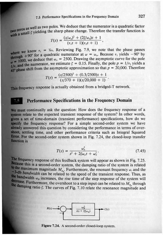
Figure 7.24. A second-order c1osed.loop system.
Performance Specifications in the Frequency Domain
327
(7.45)
C(,)R(J)
7.5 Performance Specifications in the Frequency Domain
,w.
T(s)"" , 2.s- + 2twns + W n
ney response of this feedback system will appear as shown in Fig. 7.25.this is a second-order system, the damping ratio of the system is related
. urn magnitude Mp,. Funhennore, the resonant frequency w,and thebandWidth can be related to the speed of the transient response. Thus, as
. th Wa increases, the rise time of the step response of the system will~rthe~ore. the overshoot to a step input can be related to M p" through
Ping ratIo t. The curves of Fig. 7.10 relate the resonance magnitude and
continually ask the question: How does the frequency response of arelate to the expected transient response of the system? In other words,
• set of time-domain (transient performance) specifications, how do wethe frequency response? For a simple second-order system we haveanswered this question by considering the performance in terms of over
aettling time, and other performance criteria such as Integral SquaredFor the second-order system shown in Fig. 7.24, the closed·loop transfer
is
well as twO poles. We deduce that the numerator is a quadratic factor..: ryielding the sharp phase change. Therefore the transfer function is
)(s/w.)' + (2l/w.)s + I
T(s -- (TIS + 1)(T2s + I) ,
we know 1"1 = ~o. Reviewing Fig. 7.9, we note that the phase passes+90"' for a Quadratic numerator at W "" w n• Because 1"1 yields _900 by
we deduce that W n = 2500. Drawing the asymptotic curve for the poletbc numerator, we estimate t = 0.15. Finally, the pole p "" 1/1"2 yields ashift from the asymptotic approximation so that p = 20,000. Therefore
(s/25OO)' + (0.3/25OO)s + 1T(s) - (s/370 + 1)(s/20,000 + I) .
nCy response is actually obtained from a bridged-T network.
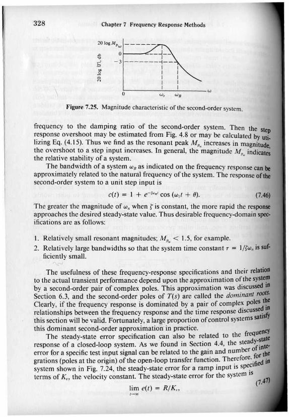
328 Chapter 7 Frequency Response Methods
201ogM, _w ,
o --l---3-------.,--
IIII
~O----~W~',-~w~,----W
Figure 7.25. Magnitude characteristic of the second-order system.
lim e(t) = RIK",-.
frequency to the damping ratio of the second·order system. Then the stepr~s'p0nse overshoot may be estimated from Fig. 4.8 or may be calculated by utj..hzmg Eq. (4.15). Thus ":,C find, as the resonant peak Mp~ increases in magnitude,the overshoot to a step mput mcrcases. In general, the magnitude AI indicatesthe relative stability of a system. p~
The bandwidth of a system WII as indicated on the frequency response can beapproximately related to the natural frequency orthe system. The response ofthesecond-order system to a unit step input is
c(t) = 1 + e~r...~, cos (Wit + 0). (7.46)
The greater the magnitude of w. when r is constant, the more rapid the responseapproaches the desired steady-state value. Thus desirable frequency·domain speo.ifications are as follows:
I. Relatively small resonant magnitudes; Mp~ < 1.5, for example.
2. Relatively large bandwidths so that the system time constant T = 18"'. is suf.ficiently smalL
The usefulness of these frequency·response specifications and their relatiOlto the actual transient performance depend upon the approximation of thes~by a second-order pair of complex poles. This approximation was diSCUssed illSection 6.3, and the second-order poles of T(s) are called the dominant ro:Clearly, if the frequency response is dominated by a pair of comp[e~ poles illrelationships between the frequency response and the time response dlscu~sl1this section will be valid. Fonunately, a large proponion ofcontrol systems saUthis dominant second-order approximation' in practice. DC'I
The steady-state error specification can also be related to the frCQUetalC
response of a closed-loop system. As we found in Sectio~ 4.4, the steadYi:owerror for a specific test input signal can be related to the gam and number 0
11rtbC
grations (poles at the origin) of the open-loop transfer funclio~. The~efore":edPIsystem shown in Fig. 7.24, the steady-state error for a ramp mput IS S~lterms of K the velocity constant. The steady-state error for the system IS 1)
" 7·( .
329
(7.53)
(7.52)
(7.51 )
(7.50)
(7.48)
(7.49)
G(jw) = (I + jWT,~1
(w./2fl K.G(s) =s(~rw.)s + I) = S(TS + I)'
G(jw) = G~) = (~),
. 5(1 + jWT2)G(jw) = jw( I + jWTI)(l + jO.6u u2) ,
.. (w;)w.K. = hm sG(s) = hm s (+ 2' ) = 2'·.-0 .-0 s S ~Wn )
7.5 Performance Specifications in the Frequency Domain
I)'Stem is type N and the gain K is the gain constant for the steady-stateus for a type-zero system that has an open-loop transfer function
+ j W72)'
(the position error constant) and appears as the low frequency gain ondiaaram.
ore, the gain constant K "" K. for the type-one system appears asthe low freqUlJncy section of the magnitude characteristic. Considering
pole and gain of the type-one system of EQ. (7.50), we have
pin constant is K. for this type-one system. F~r example, reexaminingofSection 7.3, we had a type-one system with an open-loop transfer
.K., is equal to the frequency when this portion of the magnitude charac::~rsects the O-<ib line. For example, the low frequency intersection of
tg. 7.19 is equal to W = 5, as we expect.ore ~he frequency response characteristics represent the performance. quite adequately, and with some experience they are quite useful for
and design offeedback control systems.
d,iagraIl'l form (in terms of time constants), the transfer function G(s) is
•
•• wfwn• Therefore in this case we have K. = 5. In general, if the openr function of a feedback system is written as
Krr;',(1 +jWTI)GUw) = --'-::=---
(jw)'" re~ I (I + jWTk)
R • magnitude o,f the ramp input. The velocity constant for the c1osedof Fig. 7,24 IS

330 Chapter 7 Frequency Response Methods
III Log Magnitude and Phase Diagrams
There are several alternative methods of presenting the frequency resPOnfunction GH(jw). We have seen that suitable graphical presentations of t~ ~faquency response are (J) the polar plot and (2) the Bode diagram. An alterne .re.approach ~o gra~hically portraying the frequency response is to plot the loga~~mlc magmtude In db versus the phase angle for a range of frequencies. Becathis information is equivalent to that portrayed by the Bode diagram, it is ute~al1y easier to obtain the ~ode diagram and tran.sfer the information to the c::dmates of the log magmtude versus phase dtagram. Alternatively, one canconstruct templates for first- and second-order factors and work directly on the 10f0magnitude-phase diagram. The gain and phase ofcascaded transfer functionsCIIIthen be added vectorially directly on the diagram.
-20
Figure 7.26. Log-magnitude-phase curve for GH ,Uw).
'"'"Ph.ase. degree5
,
225
00
-'0-270
-30
0.'30
03
200.6
0.0
00 w
" 2"~~ 0
~ 3.6000
-00,

Figure 7.27. log-magnitude-phasc curve for GHJUw).
331
(7.54)
-,.."225
70
7.6 Log Magnitude and Phue Diagrams
- ..-no
in FiS. 7.26. The numbers indicated along the curve are for values of........magnitude-phase curve for the transfer function
. 5(O.ljw+l)GH,(jw) ~ jw(O.5jw + IXI + jO.6(wj50) + Uwj50)') (7.55)
in Section 7.3 is shown in Fig.. 7.27. This curve is obtained mostIlly utilizing the Bode diagrams of Figs. 7.19 and 7.20 to transfer the freresponse information to the log magnitude and phase coordinates. The
jllu5U3tion will best portray the use oflhe log-magnitude-phase diagram.......p"ilUde-phase diagram for a transfer function
GH,(jw) ~ jw(O.5jw + 1~(Uwj6) + I)

(.,
x-molO' I
Melal "! beengrnved
Chapter 7 Frequency Response Methods
x Axis
Scribe
~~
The engraving machine shown in Fig. 7.28(a) uses two drive motors and associated lead screws to position the engraving scribe in the x direction. A separatemotor is used for both the y and z axis as shown. The block diagram model for
Moto•. screw andController scribe holder
~ tr c
",K 1 PoSition on
R(J) s(, + Xs + 2) X-lUis
,b'. model.
Figure 7.28. (a) Engraving machine control system. (b) Block diagram
Iksired ------1 Conlrolle.
"",,,W" ~~~~~~L Posilion measurement
_ Design Example: Engraving Machine Control System
shape of the locus of the frequency response on a log·magnitude-phase diis particularly important as the phase approaches 180· and the ma~~fllapproaches 0 db. Clearly, the locus ofEq. (7.54) and Fig. 7.26 differs SUbstan~~udefrom the locus ofEq. (7.55) and Fig. 7.27. Therefore, as the correlation betweeI:shape of the locus and the transient response of a system is establiShed"will obtain another useful portrayal of the frequency response of a syste~ ~the fo:lIowing c.hap~er, ,we will establish ,3. stability cn.reria." in the freque' adomam for which It will be useful to utilize the IOganthmlc-magnitude_Phncydiagram to investigate the relative stability of closed-loop feedback com:systems.
332

333
(7.57)
(7.56)
1.8-13
-193·
<1>("')
-135"
10
1.4-9
- 179.5·
,
1.0-4
-162"
,0.'
2T(s) = s' + 35' + 2s + 2 .
.'igure 7.29. Bode diagram for GUw).
TUw) = (2 _ 3w') : jw(2 - w') .
0.'
r------p""-------!-,soo0.'
or------~-"-~-~,,-_,_-__,--__,__,~" AsympiOlic approximaliQn
'<'
lOr<;::C-------~-----~
-lO I-'=:::::::::::------j--"'------l-"'o
Table 7.3. Frequency Response for GUw)
== 0.2 0.4 0.814 7 -I
-107· -[23' -150.5"
7.7 Design Example: Engraving Machine Control System
20108I GI
•• position control system is shown in Fig. 7.28(b). The goal is to selC{;t
. Ie gain K so that the time response to step commands is acceptablefrequency response methods.
GRIer to represent the frequency response of the system, we will fIrSt obtainp Bode diagram and the closed-loop Bode diagram. Then we will use
.Ioop Bode diagram to predict the time response of the system anddie predicted results with the actual results.order to plot the frequency response, we arbitrarily select K = 2 and pro
obtaining the Bode diagram. If the resulting system is not acceptable,later adjust the gain.frequency response of GUw) is partially listed in Table 7.3 and it is plot
Fig. 7.29. We need the frequency response of the closed-loop transfer

334 Chapter 7 Frequenc)' Response Method5
10
,~V
0
i\,10
\'I,-,
20 lac ITI. dB
0.4 0.6 0.' I0.2
· -... t-...···
-90
o
-2700.1
""igure 7.30. Bode diagram for c1osed·loop system.
The Bode diagram of the closed-loop system is shown in Fig. 7.30, where20 log I TI = 5 db at w. = 0.8. Therefore
20 log M,... = 5
0'
M,... = 1.78.
If we assume that the system has dominant second-<lrder roolS, we can appro~tmate the system with a second-order frequency response of the form shown, III
Fig. 7.9. Since MI'.. ,., 1.78, we use Fig. 7.10 to estimate po be 0.29. Using thiS rand w, = 0.8, we can use Fig. 7.10 to estimate w,jw, = 0.91. Therefore
0.8w. = 0.91 = 0.88.
Since we are now approximating T(s) as a second-order system, we have,
T(s);;;a:; w.r + 2£"w"s + w~
0.774- "'s''-+C---=O-''.5''',,=+'-0'-.7"'7'-4 .
(7. 58)

Summary
335Exercises
With increased track densities for computer disk drives, it is necessary carefully toIbe head positioning control [8}. The transfer function is
KG(s) = (s + I)l'
• POlar plot for this system when K = 4. Calculate the phase and magnitude al w =.2. and so on.
The tendon-opcrated robotic hand shown in Fig. 1.15 uses a pneumatic actuatoractuator can be represented by
G s _ 2572 2572( ) - r + 386s + 15,434 (s + 45.3)(s + 341)'
o ~uency response of G( jw). Show that the magnitude of G(jw) is -15.6 db al8Qd - 30 db at w "" 200. Also show thaI the phase is -150· at w "" 700.
this chapter we have considered the representation of a feedback control sysby its frequency response characteristics. The frequency response of a systemdefined as the steady-state response ofthe system to a sinusoidal input signal.
alternative forms of frequency response plots were considered. The polarof the frequency response ofa system G(jw) was considered. Also, logarithplots, often called Bode plots, were considered and the value of the logarithmeasure was illustrated. The ease of obtaining a Bode plot for the various
of GUw) was noted, and an example was considered in detail. The asympapproximation for drawing the Bode diagram simplifies the computation
iDlide1calbly. Several performance specifications in the frequency domain were......0;; among them were the maximum magnitude M p_ and the resonant
cy w,.. The relationship between the Bode diagram plot and the systemconstants (Kp and K,,) was noted. Finally, the log magnitude versus phase
was considered for graphically representing the frequency response of a
II use Fig. 4.8 to predict the overshoot to a step input as 37% for r = 0.29. Theing time is estimated as
4 4T, = 'w. = (0.29)0.88 = 15.7 seconds.
actual overshoot for a step input is 34% and the actual settling time is 17ds. Clearly, the second-order approximation is reasonable in Ihis case and
be used to determine suitable parameters on a system. Ifwe require a systemlower overshoot, we would reduce K to I and repeat the procedure.
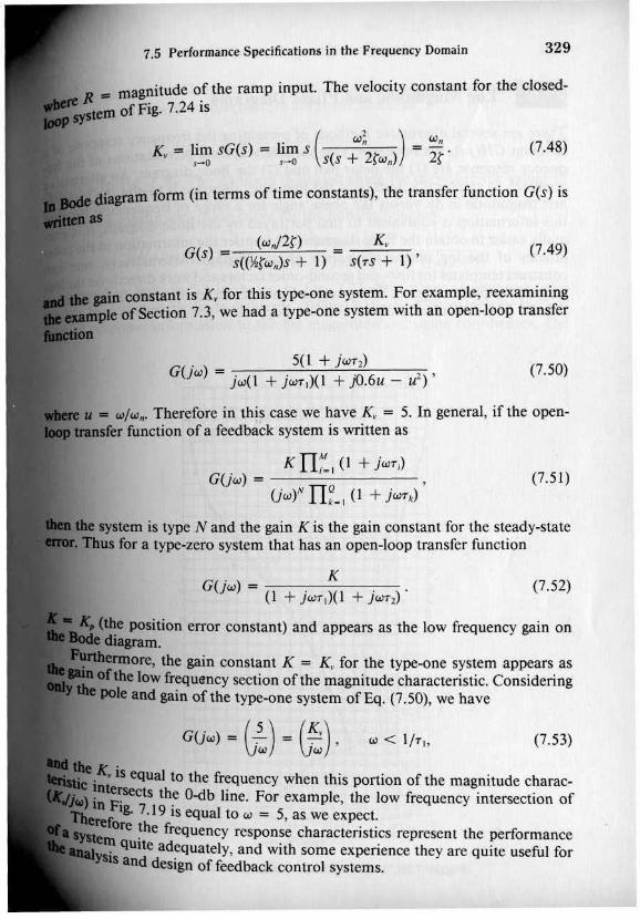
336 Chapter 7 Frequency Response Methods
£7.3. A robot arm has a joint control open-loop transfer function
G(s) _ 300($ + 100)- s(s + 10)(5 + 40)
Prove that the frequency equals 28.3 rad/sec when the phase angle ofU~) is -180". Findthe magnitude of GUr.J} al that frequency.
£7.4. The frequency response for a process of the form
G( ) Kss - (s + a)(r + 20s + 1(0)
is shown in Fig. E7.4. Determine K and a by examining the frequency response curves.
10 ~
-20
20 10@161
o
-'80"
0.' '00
Figure £7.4. Bode diagram.
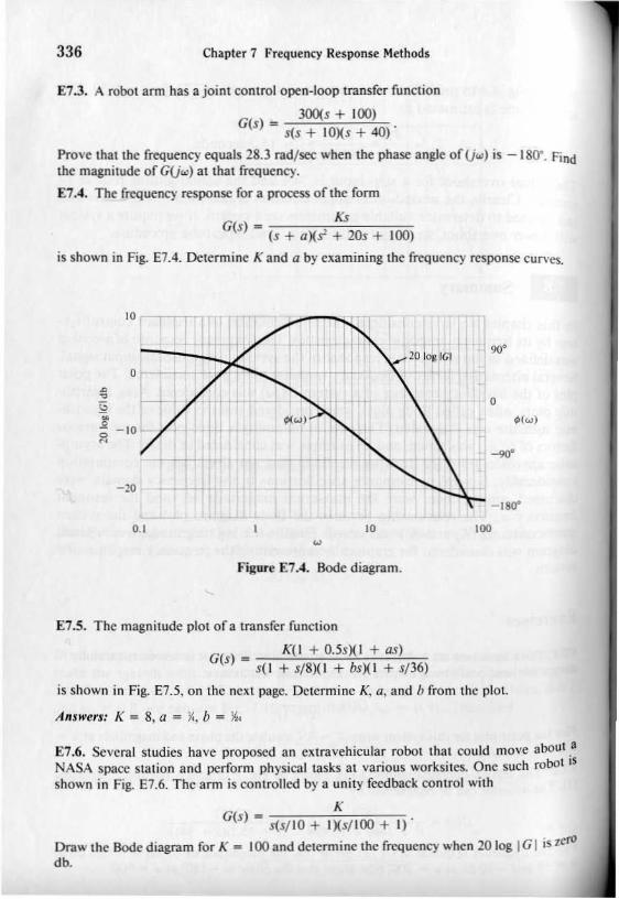
[7.5. The magnitude plol ora transfer function
G( ) K(I + 0.5$)(1 + as)S '"" s(J + s/8)(1 + bs)(l + s/36)
is shown in Fig. E7.5, on the next page. Determine K, a, and h from the plot.
A"swers: K "" 8, a e::o Yo, b '" J'.
£7.6. Several studies have proposed an extravehicular robot Ihat could move aoou1 .8
NASA space station and perform physical lasks at various worksitcs. One such robOl IS
shown in Fig. E7.6. The arm is controlled by a unity feedback control with
KG(s) - s(s/lO + IXs/IOO + I)'
Draw the Bode diagram for K _ 100 and determine the frequency when 20 log IGI is zel1l
db.

337
",
-12 db 0CI1>'C'
24 36
Exercises
Figure [7.6. Space slation robot.
Figure £7.5. Bode diagram.
•Robot arm
Robel ann
•
•
-+6 db/oclavr I-6 db/exta."c I,,
o db!oCI~'~,
, ,I I
db 1\ I I1 \ I II \ I
II \ ,I \1 II II ,I \ ,I \ ,I \ II \
"0J 4 8

Figure E7.8. (a) Head positioner (b) frequency response.
338
UnifO%Ovlp
(b)
HI.x
"1\
'1-- v1\ '\\ r \ f\
l
lU,
X= 1.37kHI. tl. Ya ..4.0711 dHYa .. -4_9411 tl.X_I.175kl-lz
Fxdyll
-30.0
339
(d) GH(,) ~ 30(, + 8)s(s + 2)(s + 4)
(b) GJ-f(s) = (I + O.5s)s'
Problems
+ 2s)
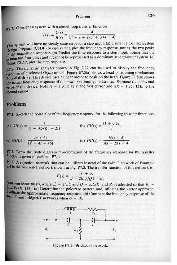
Figure P7.3. Bridged-T network.
(s + J)GH(s) = (r + 4s + 16)
~. Sketch the polar plot of the frequency response for the following transfer functions:
:.2. Draw the Bode diagram representation of the frequency response for the transfer'onsgiven in problem P7.1.
A rejection network that can be utilized instead of the lwin-T network of Example• the bridged-T network shown in Fig. P1.3. The transfer function of this network is
r + w~
G(s) = 51 + 2(w.sIQ) + w;you show this?), where w; = 21LC and Q = w.LIR. and R) is adjusted so that R1 ='i14R 1 (131. (a) Determine the pole-zero pattern and, utilizing the vector approach,
Ie the approximale frequency response. (b) Compare the frequency response of theT and bridged-T networks when Q = 10.
.1. Consider a system wilh a closed-loop transfer functionC(s) 4
T(s) = R(s) = (r + s + l)(r + O.4s + 4)'
system will have no steady-state error for a step input. (a) Using the Control SystemProgram (CSDP) or equivalent, plot the frequency response, noting the two peaks
die magnitude response. (b) Predict the time response to a step input, noting that thehas four poles and it cannot be represented as a dominant second-order system. (c)
CSDP, plot the step response.
A. The dynamic analyzer shown in Fig. 7.22 can be used to display the frequencyase of a selected G(jw) model. Figure E1.8(a) shows a head positioning mechanism
,disk drive. This device uses a linear mOlOrto posilion the head. Figure E1.8(b) showsIctual frequency response of the head positioning mechanism. Estimate the poles and
of the device. Note X = 1.31 kHz at the first cursor and 6.X = 1.257 kHz to thecursor.

figure P7.4. (a) Pressure cOnlrol1er (b) flowgraph.
-I/(s)Meas~rm:nl
chamber is sho ..." 'n
QO"'
ContrOller Valve -I 1G.V) GI(~) J PrJ,J)
450
Chapter 7 Frequency Response Methods
Controller
Infinite :==:J>k:[==~p..,_n~
IXsiredpressure
CU."') = TU"').RU",) ~
(b) Determine the ~nant frequency, "'.. (e) Determine the bandwidth of the dosedsystem.
G(s) - (I + $/2)(1 + S)(IK+ s/IO)(I + 5/30)'
where H(s) = I and K "" 10. Plot the Bode diagram of this system.
P7.6. The asymptotic logarithmic magnitude curves for two transfer functions are si:in Fig. P7.6, on the next page. Sketch the corresponding asymptotic phase shift eurves ...each system. Determine the transfer function for each system. Assume that the y11t
have minimum phase transfer functions.
P7.7. A feedback control system is shown in Fig. P7.7. The specification for the ~IOS:loop system requires that the overshoot to a step input is less than 16%. (a) Dctern\ln~corresponding specification in the frequency domain At,,. for the dosed·looP trafunction
P7.S. The robot industry in the United States is growing at a rate of JOClb a year II]· Atypical industrial robot has 5i" axes or degrees of freedom. A position control system for'force.sensingjoint has a transfer function
G,(S) :: (10 + ts).
Obtain the frequency response characteristics for the loop transfer function
G.{slG,(s)H(s) . [l/s).
P7.4. A control system for controlling the pressure in a closedFig. P7.4. The transfer function for the measuring element is
G t(S)-(O.lS+ lXI/lSs+ I)"
The controller transfer function is
H{s) "" ~ + 90s + 900"
and the transfer function for the valve is
340
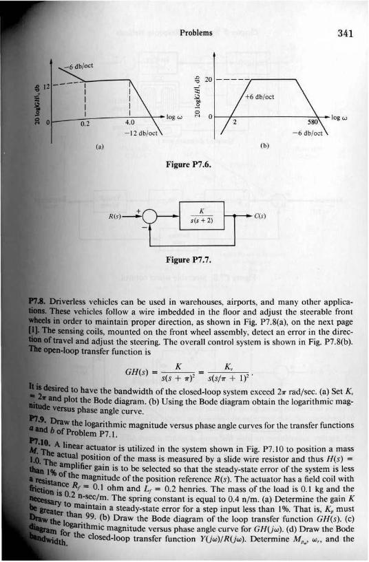
Figure P7.7.
Figure P7.6.
341
+6 db/oct
:g 20 ------~---~
(b)
Jg 0f--j!,---------:~c_Iog w
2 '"'-6 db/oct
Problems
(.)
-6 db/oct
K K,GH(s) "'" s(s + 1'ly = s(s/1r + 1)2·
to have the bandwidth of the closed-loop system exceed 2,.. rad/sec. (a) Set K,plot the Bode diagram. (b) Using the Bodc diagram obtain the logarithmic mag
phase angle curve.
the logarithmic magnitude versus phase angle curves for the transfer functionsProblem P7. I.
AIiDear actuator is utilized in the system shown in Fig. P7.IO to position a mass1ctuaJ.position of the mass is measured by a slide wire resistor and thus H(s) '""
..:pli6er sa!n is to be selectcd so that the steady-state error of the system is l~ssthe magmtude of the position reference R(s). The aclUator has a field coil WIth
it Rf .. 0.1 ohm and Lf = 0.2 henries. The mass of the load is 0.1 kg and the0.2 n-sec/m. The spring constant is equal to 0.4 njm. (a) Determine the gain K~maintain a steady-state error for a step input less than 1%. That is, Kp must
~ 99. (b) Draw the Bode diagram of the loop transfer function GH(s). (c)~thmic magnitude versus phase angle curve for GNUw). (d) Draw the Bode
the closed-loop transfer function YUw)jRUw). Determine M p_. w" and the
Driverless vehicles can be used in warehouses, airports, and many other applicaTbeee vehicles follow a wire imbedded in the floor and adjust the steerable fronlill order to maintain proper direction, as shown in Fig. P7.8(a), on the next page
ItIlSing coils, mounted on the front wheel assembly, detect an error in the direcbvel and adjust the steering. The overall control system is shown in Fig. P7.8(b).
P transfer function is
,I II II I
L_-..,','~_---,f',,-',,-'og..,0.2 4.0
-12 db/oct
Chapter 7 Frequency Response Methods
Rotor K•
KImpljr~T
X }'
344
Controllr~nsfllrmcr
('J
"100""
. t--
----"WJ
-180
-270"
-360"
"1IlOO100
~/OCI0
0~12db/OCI
0 '"-24db/~~
40
,
-40
"(b)
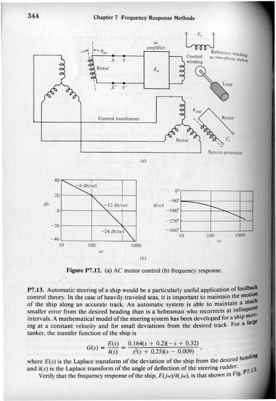
Figure P7.12. (a) AC motor control (b) frequency response.
P7.IJ. Automatic steering ora ship would be a particularly useful application offeed~oonlrollheory. In Ihe case of heavily traveled seas, it is important 10 maintain the mauoof the ship along an accurate track. An automatic system is able to maintai." a m~smaller error from Ihe desired heading than is a helmsman who recorrectS at lOfrequedintervals. A mathematical model oCthe steering system has been developed fora ship m'::ing at a constant velocity and for small devialions from the desired track. For a II...tanker,lhe transfer function oCthe ship is
G £(.1) 0.164(.1 + O.2)(-s + 0.32)(s) = il(s) - .ns + 0.25)(s 0.(09) . .
where £(s) is the Laplace transform of the deviation of the ship from lhe desired headllll
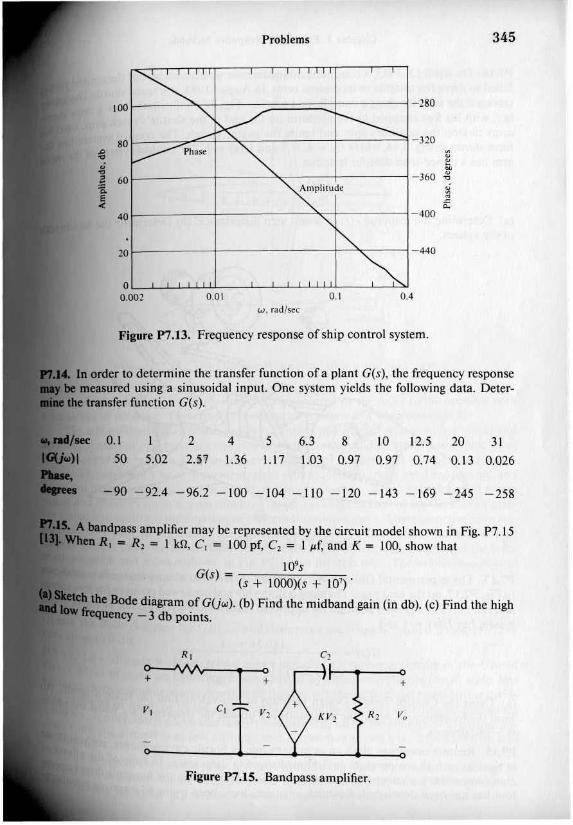
and il(s) is the Laplace transfonn of the angle of deflection of Ihe sleering ru~der. p1.1J.Verify thai the frequency response of the ship, £UIl.l)/O(jll.l), is thai shown 10 Fig.
345
20 31
0.13 0.026
+
10 12.5
0.97 0.74
8
0.97
0.1 0.4
Amplilud.
5 6.3
1.17 1.03
4
1.36
2
2.57
I
5.02
Problems
jL------l----'....---+-----1-360 ~
w. rad/<eC
L----+-----"'-+-----I-4OO
~-_.::-."':t-~--;;:=:=:=",,:±::------j -1&0
Figure P7.tS. Bandpass amplifier.
Filure P7.13. Frequency response of ship control system.
0.1SO
-90 -92.4 -96.2 -100 -104 -110 -120 -143 -169 -245 -258
,00
80PhaSl:~
t 60
~40
20
00.002 0.0\
A bandpass amplifier may be represented by the circuit model shown in Fig. P7.15R, .. R1 - I k!l, C, = 100 pr, C l = 1 ~f, and K = 100, show that
_...,..=~IO~'~s_--"",G(s) - :- (s + 1ooo)(s + 107)'
...tbe Bode diagram of GUw). (b) Find the midband gain (in db). (e) Find the high
uency - 3 db points.
In order to delennine the transfer function ofa plant G(s), Ihe frequency responsemeasured using a sinusoidal input. One system yields the following data. Deter
tile tnUlsfer function G(s).
346 Chapter 7 Frequency Response Methods
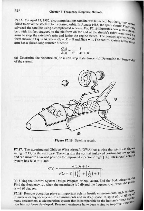
P7.16. On April 13, 1985. a communications satellite was launched but th,· .,.,-> d· h , . . .. . Ignited r L__.al cu 10 nvc 1 e sale hte to 11$ deSired Orbit. In August 1985. the space shuttle D" OC-qsalvaged the satellite using a complicated scheme. Fig. P7.16 illustrates how ISCov~
ber. with his feet strapped to the platform on the end of the shunlc's robot a c~ rn~arms to stop the satellite's spin and ignite the engine switch. The control ,,'"",• u~ bisfi h . Fi 3 semhas ......arm 5 own In Ig. .14, where G I - K - 8 and lI(s) = I. The control system orlh "'II:
arm has a closed-loop transfer function e robotC(,) 8R(s) - s: + 4$ + 8 .
(a) Determine the response c(r) 10 a unit step disturbance. (b) Determine the band .of the system. Wldth
figure P7.16. Satellite repair.
M.17. The experimental Oblique Wing Aircraft (OWA) has a wing that pivots as sboWIIin Fig. P7.17, on the next page. The wing is in the normal unskewed position ror low speedSand can move to a skewed position ror improved supersonic night [141. The aircrnrtconuol
system has H(s) "" 1 and
G(,) -C4,"(0C'.5",--,+~,)-,-_-;-
,(2, + 1) [W + (2~) + I]
(a) Using the Control System Design progrnm or equivalent, find the Bode diagram;Find the rrequency, "'I. when the magnitude is 0 db and the rrequency, "'1. when the Pis - 180 degrees.
P7.18. Remote operntion plays an important role in hostile environments. such ~~in nuclear or high-tempernlUre environments and in deep space. In spite or the c 0perrmany researchers, a teleoperation system that is comparable to the human's dircc~tion has not been developed. Research engineers have been trying to impron" tel

347
, ,
, ,
Problems
,-~
----::-4..
Maximum skcwed wing position
I
Figure P7.17. The Oblique Wing Aircraft top and side view.
IJy feeding back rich sensory information acquired by the robot 10 the operator with, of presence. This concept is called tele-existence or telepresence [ 191·
aeJe-existencc master-slave system consists of a master system with a visual andIeftSation of presence, a computer control system, and an anthropomorphic slave
DChanism with an arm having seven degrees of frecdom and a locomotion med'Ibe operator's head movement, right arm movemcnt. right hand movemcnt, and
"'<ililuy motion are measured by the master systcm. A specially designed stcreoauditory input system mounted on the neck mechanism of the slavc robot gath
and auditory information of the remote environment. These pieces of informatent back to the master system and arc applied to the specially designed stereo
I)'IIem to evoke the sensation ofpresencc of the operalOr. A diagram of the locoIYItCm and robot is shown in Fig. P7.18, on the next page. The locomotion controlbas the loop transfer
GH(s) = ,12(s + 0.5) ... +13s+30
1he Bode diagram for G/-l(jw) and detcrmine the frequency when 20 log IGN I isto odb,
~ altitude wi".d shear is a major cause of air carrier accidents in the United~ of these accidents have been caused by either microbursts (small scale. low
IQtense thunderstorm downdrafts that impact the surface and cause strong diver~fwind) or by the gust front at the leading edge ofexpanding thunderstorm
rhtt:eA nllc~oburst encounter is a serious problem for either landing or deparling air1201,lhe aircraft is at low altitudes and is traveling at just over 25% above its stall
..design of the control of an aircraft encountering wind shear after takeoff may be~ problem of stabilizing the e1imb rate about a desired value of the climb rate.
COntroller is a feedback one utilizing only climb rate information.

348 Chapter 7 Frequency Response Methods
Figure P7.18. A tele-existencc robot.
Figure P7.20. A space robot with three arms, shown capturing a satellite.'---'"
The standard negative unity feedback system of Fig. 7.24 has a loop transfer function
-'OO~G(s) - ,--,.--,-.,.,:=~-,--",-.r+ 14.r+44s+40·
Note the negative gain in G(s). This system represents the control system for climb rate.Draw the Bode diagram and determine gain (in db) when the phase is -180·,
P7.20. Space robotics is an emerging field. For the successful development of space projects, robotics and automation will be a key technology. Autonomous and dexterous spacerobots can reduce the workload of astronauts and increase operational efficiency in manymissions. Figure P7.20 shows a concept called a free-flying robot (1,19]. A major characteristic of space robots, which clearly distinguishes them from robots operated on earth, isthe lack of a fixed base. Any motion of the manipulator arm will induce reaction forcesand moments in the base, which disturb its position and auitude.
The control of one of the joints of the robot can be represented by the loop lransferfunction
GH(s) = 600(s + 6) .~ + lOs + 400

349
,
10
Problems
I [Hz]
•Figure P7.21. Motor controller.
""-""-
(.)
-30 L--.J_Ll...l.J-'..LLL_l--LLLLil.i:l01 I [Hz] 10
o
Amplifier
-'800.'
D-i(/)
Currenl oc-~
-
I Sensor I
"
pin (dBI
fib- (<leg]
Bode diagram of GHUw). (b) Determine the maximum value of 20 log IGHI,the at which it occurs, and the phase at that frequency.
tor controller used extensively in automobiles is shown in Fig. P7.21(a).~ de: m;lot of&(s)//(s) is shown in Fig. P7.21(b). Determine the transfer function
Tbe behavior of a human steering an automobile remains interesting (6,17]. The:lad development of systems for four-wheel steering, active suspensions, active,~~ing, and "drive-by-wire" steering provide the engineer with considerably
~ 10 altering vehicle handling qualities than existed in the past.vehicle and the driver are represented by the model in Fig. DP7.1, where the~ anticipation of the vehicle deviation from the center linc. For K = I, plot~m of (a) the open-loop transfer function G«s)G(s) and (b) the c1osed.]oopk. On T(~). (c) Repeat parts (a) and (b) when K = 10. (d) A driver can select
~tennlne the appropriate gain so that Alp., oS 2 and the bandwidth is theattainable for the closed-loop system. (e) Determine the steady-state error of the
ramp input, r(1) = t.
350 Chapter 7 Frequency Response Methods
G(I)Vehicle
Figure OP7.1.
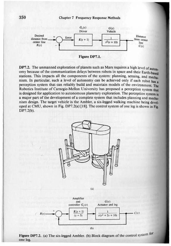
DP7.2. The unmanned expl~rati.onof planets such as Mars. requires a high level ofauIonamy because orthe commumcatlOn delays between robots In space and their Earth-basedstations. This impacts all the components of the system: planning, sensing, and m~ha
nism. In particular, such a level of au!Onomy can be achieved only if each robot has.perception system that can reliably build and maintain models of the environment. TheRobotics Institute of Carnegie-Mellon University has proposed a perception system thatis designed for application to autonomous planetary exploration. The perception system isa major pan oCthe development ofa complete system that includes planning and m~ha
nism design. The target vehicle is the Ambler, a six-legged walking machine being developed at eMU, shown in Fig. DP7.2(a) (18]. The control system of one leg is shown in FiB.DP7.2(b).
(.j
(b)
Figure DP7,2. (a) The six-legged Ambler. (b) Block diagram of the control System forone leg.
Amplifier,od
controller Gc(s)
K(s + I)
(s +5)
G(s)Actuator and leg
, f-~- CIs)s(sl + 2s + 10)
351Terms and Concepts
mqnitude The logarithm of the magnitude of the transfer function,IGI·
Plot See Bode plot.
qJue of the frequency response A pair of complex poles will result inum. value for the frequency response occuring at the resonant frequency.
,Use All the zeros of a transfer function lie in the left-hand side of
The frequency at which the frequency response has declined 3 dblow-frequency value.
The logarithm of the magnitude of the transfer function is plotted verIoprithm of !ai, the frequency. The phase, 4>, of the transfer function is
plotted versus the logarithm of the frequency.
treqaency The frequency at which the asymptotic approximation of theresponse for a pole (or zero) changes slope.
freqlleacy See Break frequency.
(db) The units of the logarithmic gain.
trauform The transformation of a function of time, f(t), into the fre·domain.
response The steady·statc response of a system to a sinusoidal input
frequency The frequency of natural oscillation that would occur for twopOles if the damping was equal to zero.
.... Phase Transfer functions with zeros in the right·hand s·plane.
Jilt A plot of the real part of G(jw) versus the imaginary part of G(jw).
resfrequency The frequency, laI" at which the maximum value of the frepOnse of a complex pair of poles is attained.
'-oction in the frequency domain The ratio of the output to the inputthe input is a sinusoid. It is expressed as G(jw).
the Bode diagram for G,(s)G(s) for 0.1 .s: w .s: 100 when K "" 20. Determinef)rIw ncy when the phase is -180· and (2) the frequency when 20 log IGG<1 =e;: the Bode diagram for the closed-loop transfer function T(s) when K = 20.
. M w" and w, for the closed-loop system when K = 20 and K = 40. (d)beSt J8i~ of the two specified in part (c) when it is desired that the overshoot of
.. to a step input, r(t), is less than 35% and the seltJing time is as short as feasible.

352
References
Chapter 7 Frequency Response Methods
l. R. C. Dorf, Encyclopedia of Robotics. John Wiley & Sons, New York. 1988.2. V. FeJiu, "Adaptive Control of a Single.Link Aexiblc Manipulator," IEEE Co
Systems. February 1990: pp. 29-32. '11'013. E. K. Parsons, "An Experiment Demonstrating Pointing Control:' IEEE Coni l
tems. April 1989; pp. 79-86. '0 Sf!_4. H. yv. ,~ode, "Relations Between Attenuation and Pha.sc in Feedback Amplifier
DesIgn, Bell System Tech. J., July 1940: pp. 421-54. Also In AII/olllatic COIl/rol- CIsical Lin~ar Theory. G. J. Thaler, cd., Dowden, Hutchinson, and Ross. Stroudsbu:Pa., 1974, pp. 145-78.
5. M. D. Fagen, A History ofEngineering and Science in the Bell System, Bell Telephl.1boralOries, Murray Hill, N.J., 1978; Ch. 3. one
6. R. A. Hess, "A Control Theoretic Model of Driver Steering Behavior," IEEE COntrolSystems, August 1990; pp. 3-S,
7. S. Winchester, "Leviathans of the Sky," Atlantic Monthly, October 1990; pp. 107-18.8. L. B. Jackson, Signals, Systems, and Trallsforms, Addison-Wesley, Reading, Masa.,
1991.9. M. Rimer and 0, K. Frederick, "Solutions of the Grumman F-14 BcnchmarkConiroi
Problem:' IEEE Control Systems. August 1987; pp. 36-40.10. K. Egilmez, "A Logical Approach to Knowledge-Based Control," J. ofime/figen/MQ~
ufac/llring, no. I, 1990; pp. 59-76.II. C. Philips and R. Harbor, Feedback Controi Systems, Prentice Hall. Englewood Clifti,
N.J.,199l.12. J. F. Manji, "Smart Cars of the Twenty-first Century," All/omation. October 1990; pP.
IS-25.13. S. Franco, Design with Operational Amplifiers and Analog integrated Cireui/$,
McGraw.Hill, New York, 1988.14. R. C. Nelson, Fligh/ Stabilily alld Automatic Control, McGraw-Hill. New York, 1989.15. R. C. Dorf and R. G. Jacquot, Control System Design Program, Addison-WesleY,
Reading, Mass., 1988.16. R. J. Smith and R. C. Oorf, CirclIits, Devices, and Systems, 5th ed., John Wiley & Sons.
New York, 1991.17. J. Krueger, "Developments in Automotive Electronics," AULOmotil'e Engineering. SeP-
tember 1990: pp. 37-44. COlt"18. M. Hebert, "A Perception System for a Planetary Explorer," Proceed. ofthe/EEE
ference on Decision and Control. 1989; pp. SO-89. .' " ()Cdfi.19. S. Tachi, "Tele-Existence Master-Slave System for Remole Manlpulatlon, P,.
ofIEEE Conference on Decision and COnlrol, December 1990: pp. 85-90. ll.;EE20. G. Leitman, "Aircraft Control Under Conditions of Windshear," Proceed. 0/
Conference all Decision and Control, December 1990; pp. 747-49. t (}If
21. K. Yoshida, "Control of Space Frce-Aying Robot," Proceed. of IEEE Con!erenc
Decision and Con/rol, December 1990; pp. 97-101. . .. acted. 0/22. T. Kawabe, "Controller for Servo Positioning System of an AutomobIle, pr
IEEE Conference on Decision and Control, December 1990; pp. 2170-74.,