Formal Analysis of DeGroot Influence Problems using

Probabilistic Model Checking

Sotirios Gyftopoulosa,∗, Pavlos S. Efraimidisa, Panagiotis Katsarosb

aDept. Electrical & Computer Engineering Democritus University of Thrace Office 4,Building A, University Campus 67100 Xanthi, Greece

bDepartment of Informatics Aristotle University of Thessaloniki, 54124 Thessaloniki,Greece

Abstract

DeGroot learning is a model of opinion diffusion and formation in a social

network. We examine the behavior of the DeGroot learning model when

external strategic players that aim to influence the opinion formation process

are introduced. More specifically, we consider the case of a single decision

maker and that of two competing players, with a fixed number of possible

influence actions for each of them. In the former case, the DeGroot model

takes the form of a Markov Decision Process (MDP), while in the latter case

it takes the form of a Stochastic Game (SG). These models are solved using

probabilistic model checking techniques, as well as other solution techniques

beyond model checking. The viability of our analysis is attested on a well

known social network, the Zachary’s karate club. Finally, the evaluation of

influence in a social network simultaneously with the decision maker’s cost is

supported, which is encoded as a multi-objective model checking problem.

Keywords: Social networks, Opinion dynamics, DeGroot model, Stochastic

games, Probabilistic model checking, Zachary karate club

∗Corresponding authorEmail addresses: sgyftopo@ee.duth.gr (Sotirios Gyftopoulos),

pefraimi@ee.duth.gr (Pavlos S. Efraimidis), katsaros@csd.auth.gr (PanagiotisKatsaros)

Preprint submitted to Elsevier May 12, 2019

1. Introduction

Opinion dynamics is the field of research on the process of opinion dif-

fusion among individuals and on models that incorporate rules of opinion

formation. Various models have been introduced that imitate the under-

lying principles of opinion diffusion [1, 2, 3] and are being analyzed [4], in

order to determine elaborate characteristics of opinion formation and ways

to influence the diffusion process.

In 1974, Morris H. DeGroot introduced a model known as the DeGroot

model [1], in which individuals participate in a social network with friend-

ships. Every individual is averaging his own opinion with those of his friends

iteratively, until the process converges. The location of each individual in

the network is of vital importance for the prevalence of his opinion in the

consensus, since the averaging of opinions highlights the importance of cen-

trality in the network. His friendships with other members determine his

contribution in the consensus and, consequently, his centrality in the opinion

diffusion process. Thus, the model incorporates elaborate characteristics of

the opinion formation process and provides solid ground for experimentation.

DeGroot remarked that the averaging process of opinion propagation can

be interpreted as a Markov chain and used theorems from Markov chain

theory to determine the conditions under which his model converged.

The common mathematical underpinnings of the DeGroot model and

Markov processes allow for automating the analysis of DeGroot social net-

works by utilizing a multitude of software tools [5, 6, 7, 8] for the verification

of important probabilistic properties [4]. We specifically focus on the use of

probabilistic model checking techniques [9], but we also explore the efficiency

of other analysis techniques implemented in a mathematical solver.

2

In [10], we introduced variants of the DeGroot model, which allow study-

ing the impact of external influence on the opinion formation process. The

classical DeGroot Problem (DP) and the so-called DeGroot Influence Problem

(DIP) and DeGroot Game (DG) were formalized into a probabilistic model

checking framework. Our approach allows to extract the strategies that ex-

ternal players could develop, in order to interfere with the process and the

individuals’ influence in the final consensus. We opted to experiment using

the PRISM model checker [5] and the PRISM-games extension [7], due to

the wide range of provided functionalities. Their modelling language offered

a human-friendly environment for the construction of DP , DIP and DG

models and their property language incorporated the necessary operators for

elaborate analysis of the models’ characteristics. Furthermore, the graphical

user interface enabled the extraction of the external players’ strategies in the

cases of DIP and DG.

In the current article, we introduce a multi-objective variant of the DeG-

root model, the Constrained DeGroot Influence Problem (CDIP), for study-

ing simultaneously the external influence in a social network and its associ-

ated cost. Furthermore, we analyze our variants of the DeGroot model with

other solution techniques beyond model checking and we apply our models

on a well studied real life social network. The concrete contributions of our

work can be summarized as follows:

1. we provide sound theoretical foundation of theDIP probabilistic model

checking approach and additional experimental results for the interven-

tion of a strategic entity in the consensus formation process with respect

to his range of influence;

2. we present the CDIP model, a multi-objective generalization of the

DIP problem, for studying the trade-off between influence in a social

3

network and cost in the case of one strategic entity;

3. we analyze other solution techniques beyond model checking and and

provide a comparative evaluation in terms of efficiency and ease-of-use;

4. we present an application of our models and experimental results on a

well known real life social network, the Zachary’s karate club [11].

The implemented models used in this work along with other supplemen-

tary material can be accessed online1.

The extensions of the DeGroot model offer new perspectives in the anal-

ysis of modern practical problems such as those faced in targeted marketing.

In this particular field, the focus is on how to utilize the available features of

modern social media, in order to attract customers and establish the position

of brands in the market [12, 13, 14]. Recent research aims to innovative direc-

tions in the development of marketing strategies that promote the selection

of the most influential nodes in a social graph [15, 16]. Moreover, our DeG-

root model extensions and their solutions provide a novel prism for analysis

of DeGroot modeling problems, such as the product recommendation system

of [17], for the users of online stores.

The paper is organized as follows: Section 2 lists recent findings of re-

lated works in the field of opinion diffusion, model construction and simula-

tion. Section 3 presents concise descriptions of the DeGroot model, stochastic

games and the model checking problem. In Section 4, we describe the im-

plementation of the DeGroot model and Section 5 presents extensions of the

DeGroot model and experimental results. Section 6 summarizes the findings

and restrictions that are highlighted by our experiments.

1The models can be found here: http://euclid.ee.duth.gr/degroot-pmc/

4

2. Related Work

A comprehensive analysis of the most popular opinion diffusion models

was presented in [4]. DeGroot learning was considered as the classical opinion

diffusion model, while various extensions were analyzed without studying the

external influence and the strategic aspects of DeGroot learning, as we do

in this work. Two other models were also presented, namely the Friedkin

and Johnsen model [2], and the Bounded Confidence (BC) model [18]. The

behavior of the consensus formation process for the BC model was analyzed

using simulation, which allows to study the characteristics of the original

model and its variants. Computer simulation using, e.g., Matlab was also

employed in other studies of opinion diffusion models such as the one in [19].

In [20], a model of coevolution of networks and opinions, that resembled

the DeGroot model, was presented. More specifically, while in the DeG-

root model each node updates its opinion by averaging the opinions of its

neighbours, in [20] a node either convinced one of its neighbours to adopt its

opinion or befriended with a node hosting a similar opinion. The character-

istics of the convergence to consensus state were studied through computer

simulation. A more recent study of the same model was also presented in

[21], where the authors mainly employed analytical techniques.

The Deffuant model [22] was analyzed in [23] through regression analysis,

where the model’s convergence time was expressed as a function of various

parameters.

However, we are not aware of any related works that focus on the external

influence and the strategic aspects of DeGroot learning using probabilistic

model checking techniques. Works that are somehow related in that they

use probabilistic model checking but address different problems are [24] and

[25]. In [24], the authors used probabilistic model checking to analyze the

5

evolution of a disease spread over groups of people. The variations of the

spread depending on the possible vaccination strategies were analyzed based

on a Continuous Time Markov Chain (CTMC). In [25], a social graph con-

sisting of multiple avatars of users in different social networks was modeled

as a Discrete Time Markov Chain (DTMC) and PRISM was used to ana-

lyze simple characteristics of the model (e.g., the probability of information

leakage). Properties of the model were evaluated to investigate the spread of

information over “detached” users of social networks.

3. Preliminaries

3.1. The DeGroot Model

In the DeGroot model, each individual has an initial opinion and a set of

friends with whom he shares his opinion. After the opinions are exchanged,

an update process takes place that averages each individual’s opinion with

those of his friends; the range of trust in his friends’ opinions may vary.

Under plausible conditions, the opinions of all members converge after a

sufficient number of iterations [1]. The consensus depends on the social

group structure, i.e., the factors of trust among the individuals.

4

5

2

3

1 6

1

2

1

2

1

4

1

4

1

4

1

4

1

4

1

6

1

6

1

6

1

3

1

3

1

3

1

2

1

4

1

2

1

2

1

2

Figure 1: A social network with six members.

6

A social group is depicted by a social graph, in which individuals are

represented by nodes and their friendships by directed edges (i.e., incident

arcs) to other nodes. As shown in Figure 1 for a six-member social network,

the weights in outgoing arcs of a node are summed to 1 and represent the

range of trust of the group member to the opinions of his neighbors. Every

node is neighbor with itself, thus defining the node’s self-confidence. The

weights are used in the opinion update process, where the updated opinion

of a node is the weighted average of opinions that are taken into account. In

Figure 1, some nodes value their own opinions more (e.g., nodes 2 and 4),

while others distribute their averaging factors uniformly to their neighbors

(e.g., nodes 1, 3, 5 and 6).

In terms of linear algebra, the graph of Figure 1 is represented by a 6 ×

6 adjacency matrix P , where each element pij denotes the averaging factor

of node i to node j. If F0 is the vector of initial opinions for the nodes, then

the averaging process of DeGroot model is captured as follows:

Fn = PFn−1 = P nF0 (1)

where Fn and Fn−1 represent the opinion vectors after n and n− 1 iterations

respectively, of the averaging process.

DeGroot remarked in [1] that P can be interpreted as the one-step tran-

sition matrix of a Markov chain and applied the standard limit theorems of

Markov chains theory to determine its convergence.

3.2. Stochastic Games

Stochastic games were introduced by Shapley [26] as a formal model which

incorporates actions and payments for two strategic players interacting on a

finite set of N game states. The two players choose their actions i and j in

state k from the sets of available actions Mk and Nk for them respectively and

7

the next state l is determined probabilistically depending on their actions.

The probability of reaching state l from k is pklij . The stopping factor skij > 0

for each state k denotes the probability that the game stops after the players

make their moves. In all cases, the game ends after a finite number of steps,

since∏∞

t=1(1− stij)→ 0.

The model also includes payoffs for the players in the form of payments

from one player to the other. The payment akij at state k is determined based

on the ith and jth actions of the players in this state. The sum of payments akij

and−akij, for the two players, is 0 (zero-sum game). Players have incentives to

choose their actions accordingly, for maximising their long-term payoff, thus

developing strategies that indicate their moves in every game state. The value

val of a game is the minimum expected payoff for a player, when applying an

optimal strategy, regardless of the other player’s strategy. Optimal strategies

are stationary, i.e., every next action depends only on the current game state

(the history of previous states is irrelevant). It has been shown that the value

of a stopping game converges, as the game’s duration increases (e.g., through

a decrease of the stopping factor) [27].

Stochastic games can be considered as a generalization of Markov De-

cision Processes (MDPs), which are solved in polynomial time using, e.g.,

dynamic or linear programming [28, 29]. MDPs represent the intervention

of a strategic entity (the decision maker) in a specific environment. The

introduction of a second strategic entity transforms the model to a stochas-

tic game. Markov chains can be perceived as stochastic games, where both

players have no alternatives in the game states.

3.3. Model Checking

Probabilistic model checking is an automated verification technique that

combines graph-theoretic algorithms for reachability analysis with iterative

8

numerical solvers. Model-checking tools like PRISM [5] can evaluate proper-

ties in PCTL (Probabilistic Computational Tree Logic) of the form Ponq(ψ),

for on∈ {<,≤,≥, >}, q ∈ Q ∩ [0, 1] (Q is the set of rational numbers) or

P=?(ψ), which compute the probability that a path satisfies ψ. The path

formula ψ is interpreted over the paths of a probabilistic model, which can

be a DTMC, a CTMC, or an MDP. The semantics of Ponq(ψ) over MDPs

is that, for all strategies, the probability that ψ is true for a path satisfies

on q, where a strategy (or adversary) for an MDP is a function mapping

that resolves nondeterminism between the possible actions based on exe-

cution history. The model checking of such properties is reduced to the

computation over all strategies of the minimum/maximum probability for ψ

holding true. Two forms of quantitative properties for MDPs are supported

by PRISM, namely Pmin=?(ψ) and Pmax=?(ψ). PRISM-games [7] is an exten-

sion of PRISM that supports the formulation and the analysis of turn-based

(i.e., a single player can make a move in each state) stochastic games played

between two (coalitions of) players.

Probabilistic model checkers also allow defining reward structures as:

(i) state rewards (ρ : S → R≥0) and (ii) transition rewards (ι : S×S → R≥0),

where S is the set of model’s states. For DTMCs, reward properties are stated

using the R operator, as R {"rewardId"} on x [ψ] or R{"rewardId"} =? [ψ],

where rewardId refers to the used reward structure and ψ is a path formula.

Such a property returns the instantaneous (or cumulative) expected reward

for the reward structure, until the path formula is true. For MDPs, rewards

can be assigned to actions instead of transitions and the respective properties

take the form R{"rewardId"}max =? [ψ] or R{"rewardId"}min =? [ψ].

PRISM-games supports an extension of rPATL (Probabilistic Alternating-

time Temporal Logic with Rewards) adequate for quantitative properties of

9

stochastic games with rewards. We can write coalition-based properties that

identify optimal strategies, with respect to the expected probability of a path

or the expected value of accumulated reward, until reaching a set of states.

PRISM and PRISM-games also provide2 the necessary functionalities for

the analysis of multi-objective properties [30]. Such properties enable the

exploration of trade-offs between measurable quantities (e.g., performance

and resource requirements) and are expressed as a Boolean combination of

objectives in the form of expected total rewards, expected mean-payoffs or

ratios of expected mean-payoffs. Multi-objective properties can be evaluated

in terms of their achievability, their numerical values and their Pareto curves

[31].

4. The DeGroot Model As A Stochastic Process

4.1. The DeGroot Problem (DP)

The DeGroot Problem DP is defined as a tuple (G 〈N,P 〉 , B0), where

G is a graph with nodes N = {1, ..., n}, P is a n × n stochastic matrix

(also called adjacency matrix [32]) and B0 = [b01 . . . b0n] is a vector of initial

opinions of the nodes in N on a specific matter of interest (beliefs as real

values ranging from 0 to 1). The element pij of P represents the link weight

of node i to node j that is used in i’s opinion update process. If two nodes

are not linked, P ’s corresponding element is zero. In the DeGroot model,

P ’s elements represent the factors of the weighted averaging process.

Given a DP = (G 〈N,P 〉 , B0) our goal is to evaluate the final opinion in

state of consensus. The influence of each node is determined by the eigenvec-

tor centrality of the node. Solving such a model is a problem of polynomial

2PRISM version 4.4 and PRISM-games version 2.0.beta3

10

4

5

2

3

1 6

0.ത3

0.5

0.5

0.5

0.5

0.5

0.25

0.5

0.25

0.25

0.25

0.250.25

0.ത3

0.ത3

0.1ത6

0.1ത6

0.1ത6

Figure 2: Graph G∗ of DP ∗ and the elements of P ∗

complexity [33]. Relevant algorithms have been studied especially in the

context of the popular PageRank centrality [34].

Figure 2 shows the social graph of an example DP ∗ = (G∗ 〈N∗, P ∗〉 , B∗0)

that we modeled [10] as a DTMC in PRISM. The DTMC consisted of six

states that represented the six nodes of G∗ and state transitions as defined by

P ∗; a reward structure represented the nodes’ opinions, which were initially

set to 0.5 except the opinions of nodes 1 and 6, which were set to 0 and 1

respectively. DP ∗ reached a consensus after an adequate number of opinion

updates. The consensus formation process was analyzed using the property

of Listing 1, with the R operator for the accumulated rewards (i.e., opinions)

in the steady state (operator S).

R=? [ S ]

Listing 1: Property of DTMC model for DP ∗

PRISM offered the necessary functionality to extract the stationary prob-

ability vector π as DeGroot defined it in [1]. The stationary probability

vector π is the solution of Equation 2.

πP ∗ = π (2)

11

Table 1: Vectors π of DP ∗, π′ of DIP ∗, π′′ of DG∗ and the final opinions.

Node Opinion Factors of π Factors of π′ Factors of π′′

1 0 0.2045 0.3943 0.2232

2 0.5 0.0454 0.0343 0.0322

3 0.5 0.2727 0.3086 0.2594

4 0.5 0.1363 0.0617 0.0773

5 0.5 0.2272 0.1509 0.2447

6 1 0.1136 0.0503 0.1631

Final opinion 0.45454 0.32800 0.46994

The consensus b∗c of G∗ can be computed using π and the vector B∗0 of initial

opinions of the nodes:

b∗c = πB∗0 (3)

Vector π and the extracted consensus of DP ∗ are presented in Table 1 along

with π′ and π′′ which are discussed in Sections 5.1 and 5.5.

4.2. DP for Zachary’s Karate Club

In [11], Wayne W. Zachary presented a social network with members of

a karate club that was fissioned due to their disagreement over the lessons’

price. The club was observed for three years before being modeled. It initially

included 34 members, whose connections were recorded. After the fission, two

clubs were formed, one headed by the karate instructor and one administered

by the initial club’s officer. Zachary’s research aimed to model the structure

of the network and to apply the maximum flow - minimum cut procedure

[35], in order to collate the findings with the real data of the fission.

The dataset of Zachary’s research provides the adjacency matrix (exis-

tence matrix E) of the network, as well as its weighted version (capacity

matrix C). Zachary assigned weights to each connection of the network

12

based on the context of the members’ interaction. Figure 3 depicts the social

network of Zachary’s karate club as an undirected graph without weights for

convenience purposes.

10

151619

21

23

24

25

26

27

28 29

32

30

31

34

33

1

2

3

4

5

6

7

8

9

12

13

11

14

1718

2022

Figure 3: Zachary’s karate club as an undirected social network. Members of the two

clubs, that were formed after the fission, are depicted in different shapes and colors (blue

circles and orange squares).

The social network of our implementation of the DP on Zachary’s karate

club is based on the existence matrix E from [11]. E can by viewed under

the prism of trust of a node to its neighbours’ opinions. The original version

of Zachary’s karate club does not take into account self-confidence, that is

not likely in opinion diffusion models. This drawback can be overcome by

adopting the assumption that each member has by default a certain degree

of trust in his opinion. We conjecture that each node is equally influenced

by its own opinion and its neighbours’ opinions and we assign to elements eii

of E a value equal to the sum of other elements of the ith row.

In order to comply with the formulation of the DeGroot model, the

weights are normalized such that the total outgoing weight of each node

13

is 1. The opinions used in our implementation are determined by the club

that each member chose to join after the fission. The members that joined

the instructor’s club (node 1) are assigned an opinion of 1 forming, thus, the

instructor’s sphere of influence, while the members that joined the officer’s

club (node 34) are assigned an opinion of 0 and correspond to the officer’s

sphere of influence. With these opinions we intent to capture the state of the

social network shortly before the fission.

Under the above assumptions, we defined the tuple DPZ = (GZ〈NZ , PZ〉,

BZ0) and implemented it in PRISM. The members of the social network

are represented as nodes of a graph and a random walk is used to emulate

the averaging process of the DeGroot model. The evaluation of the property

that provides the consensus reveals a final opinion (b∗Zc) of 0.519231. We note

that the two clubs that were formed after the fission had both 17 members,

therefore a consensus of 0.519231 is in agreement with the separation of the

members.

5. DeGroot Model Extensions As Stochastic Processes

In this section, we extend the DP by including strategic entities that aim

to manipulate the consensus formation process. We present concisely the

DeGroot Influence Problem (DIP) and the DeGroot Game (DG), that were

introduced in [10], and we provide additional experimental results regarding

the impact of the strategic entities’ interference. Furthermore, the newly

presented Constrained DeGroot Influence Problem (CDIP) focuses on the

trade-off between influence and cost for the strategic entity.

5.1. The DeGroot Influence Problem (DIP)

In the DeGroot Influence Problem (DIP), a strategic entity (i.e., decision

maker) D aims to tamper with the consensus formation process of the DP .

14

42

1

1

4+ 𝑘

1

2

1

4

42

1

1 + 4𝑘

4 + 4𝑘

1

2 + 2𝑘

1

4 + 4𝑘

Figure 4: (a) The decision maker D chooses action a21 = k (b) The distribution of all

p2j , j ∈ N is reformed after the normalization process.

The problem is defined as a tuple (G 〈N,P 〉 , B0, D 〈A, t〉) where G is a graph

with nodes N = {1, ..., n}, P is a n×n stochastic matrix that corresponds to

the adjacency matrix of G, B0 = [b01 . . . b0n] is a vector of initial opinions of

the nodes in N , A is the set of actions available to D and t the target opinion

of D. Set A consists of real-valued elements aij for an action j that D can

undertake on node i to alter the value of pij in P . The decision maker can

only alter the weight of existing links in G, i.e., aij ∈ A ⇔ pij > 0 (actions

for creating additional links can be supported at the expense of increased

computational complexity as explained in Section 5.7).

Figure 4 illustrates the undergoing changes as a consequence of an action

aij by D. Let us consider that the chosen action is a21 = k. The p21 = 14

is

increased by the factor k and D thus enhances the opinion of node 1 in the

update process of node 2 (Figure 4a). However, the extra value k increases

the sum of weights of node’s 2 outgoing arcs to 1 + k enforcing, thus, a

normalization process for all p2j > 0, j ∈ 1, . . . , n to comply with the weighted

averaging process of the DeGroot model for graph G. The normalization

alters the distribution of node’s 2 factors by increasing p21, while decreasing

p22 and p24 (Figure 4b). Thus, a single action causes the alteration of the

stationary probability vector π of the graph, which represents the distribution

15

of influence in the social network.

Factor k represents the impact of the influence wielded on an existing link.

A large k in the example of Figure 4 implies a dominant role on the link,

where the action is applied to, suppressing the contribution of the rest of the

links in the opinion update process and, consequently, causing the opinion

of the node to be dominated by a single neighbour. A positive k represents

an enhancement of the link, while a negative k would imply an attenuation

of the link’s contribution in the opinion diffusion. The update rule imposes

positive weights for all links, a condition that should be preserved in case of

a negative k. Moreover, the application of an action should not disturb the

stochasticity of the matrix when a normalization process is applied. These

restrictions imply that the lower limit of k in A is determined by the link

with the lowest weight pmin: in case factor k has a lower value than −pmin,

then the application of an action on the corresponding link would result in

a negative weight disturbing, thus, the stochasticity of matrix P when the

normalization is applied.

D is urged to select the proper actions aij in order to influence the con-

sensus of G towards t. Hence, D aims to construct an optimal strategy

σ = {aij|aij ∈ A} that would alter the stationary probability vector π into

π′ to achieve the maximum prevalence of the nodes with opinions close to t

in the consensus formation. D can choose only one action for every node of

the graph, thus for any two aij, akl ∈ σ, i = k =⇒ j = l. By definition,

the optimal strategy σ is stationary, i.e., it consists of actions that cannot

be changed during the consensus formation process.

In [10], we modeled an example DIP ∗ = (G∗ 〈N∗, P ∗〉 , B∗0 , D∗ 〈A∗, t∗〉)

as an MDP in PRISM. Graph G∗ and opinion vector B∗0 were the same as in

the DP ∗ of Section 4.1. D∗ was provided with a set A∗ of actions a∗ij such

16

that k = 0.25, for all existing arcs of G∗, whereas the target opinion t∗ was

set to 0. Our model allowed D∗ to manipulate the transition matrix in order

to interfere with the opinion diffusion. Our aim was to enable D∗ to generate

an optimal strategy σ∗ that promoted his target opinion t∗ hosted by node

1 (see Table 1).

In PRISM, there is no direct way to extract the stationary optimal strat-

egy (policy) for an MDP that would allow studying the resulting DTMC in

the steady state. However, since a Markov chain can be interpreted as a ran-

dom walk through its states, we can deduce that the values of π are identical

to the corresponding probabilities of the random walk reaching each state

(i.e., node of the graph) in an infinite path. Using PRISM’s functionality,

we can extract an optimal strategy for the value of a property in finite steps

of control by the decision maker (planning horizon) that emulate a random

walk on the graph. Through this approach, we obtained an ε-optimal strat-

egy for a property, thus having evaluations with accuracy at least ε. We

show (the proof of Proposition 1 is in Appendix A) that such a strategy that

minimized the cumulative and, hence, the average reward, is identical to the

optimal strategy that minimized the average reward over the infinite plan-

ning horizon, provided that the finite horizon’s length was sufficiently long

(i.e., its steps exceeded an appropriate number).

Proposition 1. Assume a Markov Decision Process with state space X, ac-

tion set A, reward structure rti(a) that assigns instantaneous rewards at time

point t when the process is at state i ∈ S, and the set of stationary strategies

or policies ΠS. There exists a time point tL such that, for all t > tL, if policy

π∗ ∈ ΠS minimizes the cumulative expected reward of the MDP over finite

planning horizons with length greater than tL, then policy π∗ minimizes the

average reward of the MDP over the infinite planning horizon.

17

For the PRISM model of DIP ∗, the planning horizon was determined by

the random walk’s steps. To the best of our knowledge, there are no analyt-

ical tools to find the minimum length of a random walk for guaranteeing the

extraction of optimal strategy. Therefore, we used walks with λ = 1000000

steps, which we experimentally confirmed that provided ε-optimal strategies

for our model with ε < 10−5. The adequacy of λ was also confirmed with

a mathematical solver [8] for MDPs (the extracted optimal strategy of the

mathematical solver coincided with the ε-optimal strategy of our model).

Certainly, the walk’s length may vary for different applications, as its ad-

equacy depends on the MDP model. Variations in transition probabilities

and in the state space may require adjustments in λ for computing ε-optimal

strategies.

The optimal strategy of the decision maker for the PRISM model of the

DIP ∗ was constructed using the property of Listing 2. Under this strategy,

the opinion of the DIP ∗ model in state of consensus was evaluated with ε

accuracy. The C operator corresponded to the accumulated rewards (i.e.,

opinions) in our random walk, whose length was set to const lamda. To

extract the actions of the optimal strategy, the MDP was reformulated as a

stochastic game, in order to use the available functionality in PRISM-games.

const i n t lamda = 1000000;

Rmin = ? [ C <= lamda ] / lamda

Listing 2: Property of DIP ∗ model

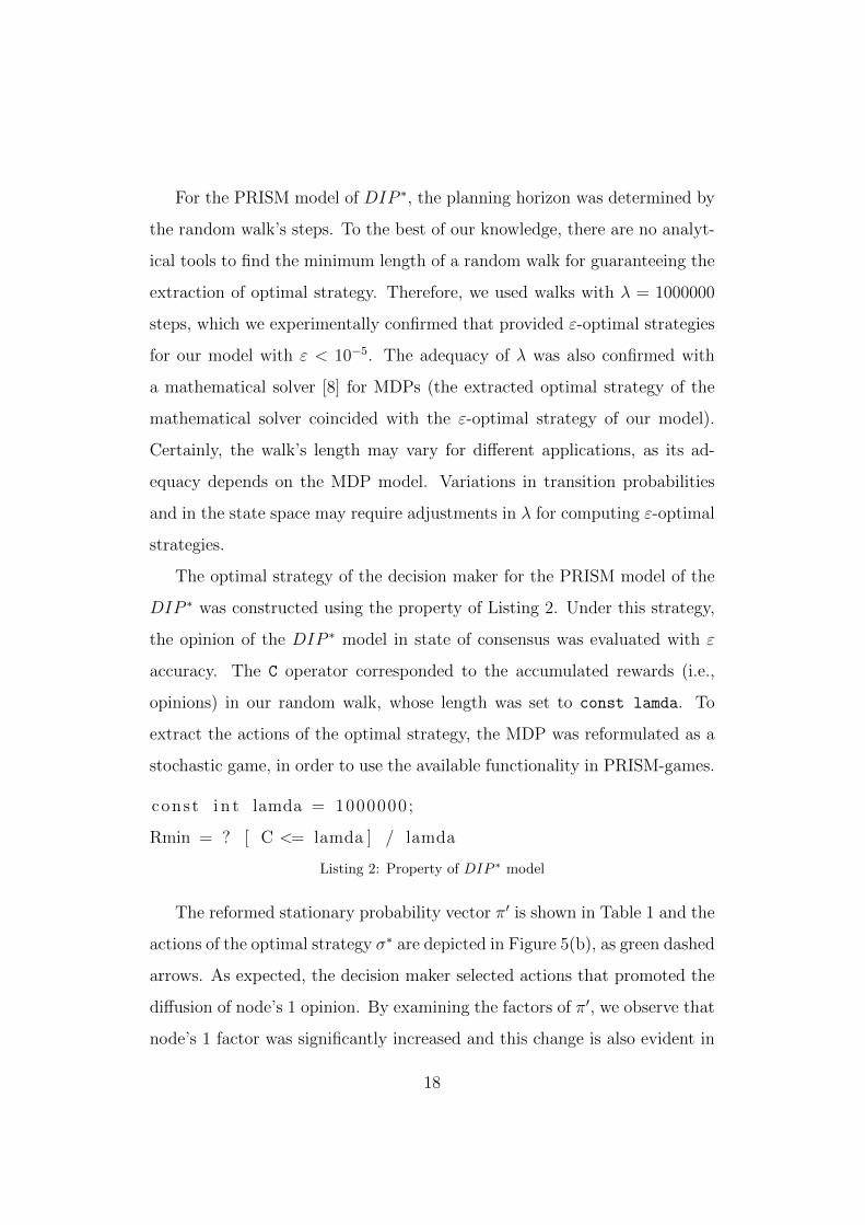
The reformed stationary probability vector π′ is shown in Table 1 and the

actions of the optimal strategy σ∗ are depicted in Figure 5(b), as green dashed

arrows. As expected, the decision maker selected actions that promoted the

diffusion of node’s 1 opinion. By examining the factors of π′, we observe that

node’s 1 factor was significantly increased and this change is also evident in

18

4

5

2

3

1 6

4

5

2

3

1 6

Figure 5: Graph G∗ of DIP ∗ and strategy σ (red and green dashed arrows) of the decision

maker:(a) for k=-0.16, (b) for k=0.25.

its neighbouring node 3. The factors of the other nodes were decreased and

the consensus was decreased, as intended by the decision maker.

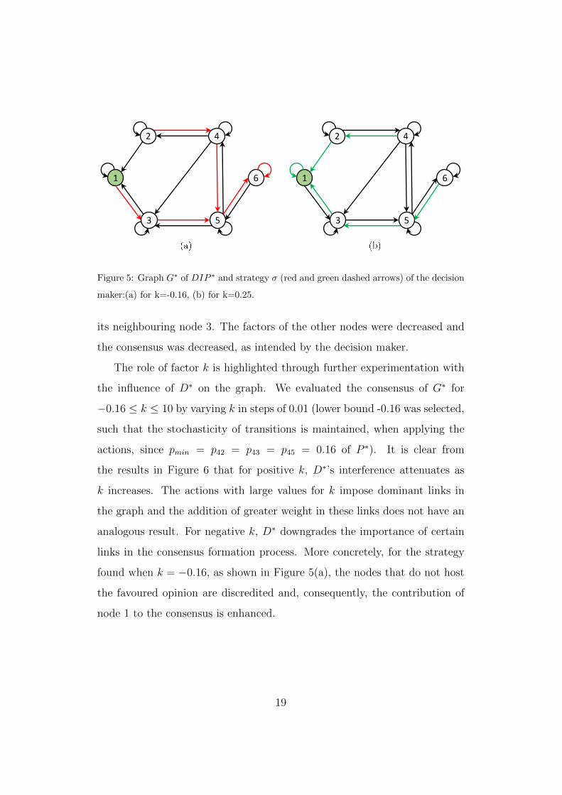
The role of factor k is highlighted through further experimentation with

the influence of D∗ on the graph. We evaluated the consensus of G∗ for

−0.16 ≤ k ≤ 10 by varying k in steps of 0.01 (lower bound -0.16 was selected,

such that the stochasticity of transitions is maintained, when applying the

actions, since pmin = p42 = p43 = p45 = 0.16 of P ∗). It is clear from

the results in Figure 6 that for positive k, D∗’s interference attenuates as

k increases. The actions with large values for k impose dominant links in

the graph and the addition of greater weight in these links does not have an

analogous result. For negative k, D∗ downgrades the importance of certain

links in the consensus formation process. More concretely, for the strategy

found when k = −0.16, as shown in Figure 5(a), the nodes that do not host

the favoured opinion are discredited and, consequently, the contribution of

node 1 to the consensus is enhanced.

19

0.00

0.05

0.10

0.15

0.20

0.25

0.30

0.35

0.40

0.45

0.50

-1 0 1 2 3 4 5 6 7 8 9 10

Figure 6: The consensus of G∗ for −0.16 ≤ k ≤ 10

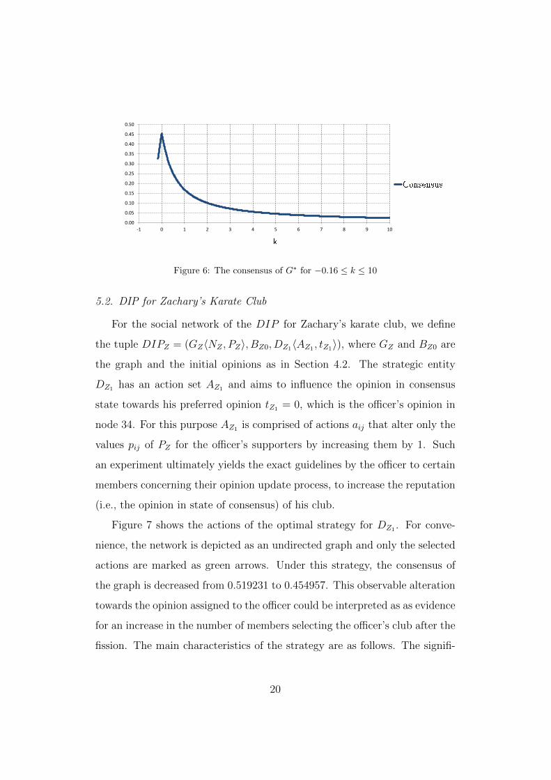
5.2. DIP for Zachary’s Karate Club

For the social network of the DIP for Zachary’s karate club, we define

the tuple DIPZ = (GZ〈NZ , PZ〉, BZ0, DZ1〈AZ1 , tZ1〉), where GZ and BZ0 are

the graph and the initial opinions as in Section 4.2. The strategic entity

DZ1 has an action set AZ1 and aims to influence the opinion in consensus

state towards his preferred opinion tZ1 = 0, which is the officer’s opinion in

node 34. For this purpose AZ1 is comprised of actions aij that alter only the

values pij of PZ for the officer’s supporters by increasing them by 1. Such

an experiment ultimately yields the exact guidelines by the officer to certain

members concerning their opinion update process, to increase the reputation

(i.e., the opinion in state of consensus) of his club.

Figure 7 shows the actions of the optimal strategy for DZ1 . For conve-

nience, the network is depicted as an undirected graph and only the selected

actions are marked as green arrows. Under this strategy, the consensus of

the graph is decreased from 0.519231 to 0.454957. This observable alteration

towards the opinion assigned to the officer could be interpreted as as evidence

for an increase in the number of members selecting the officer’s club after the

fission. The main characteristics of the strategy are as follows. The signifi-

20

10

151619

21

23

24

25

26

27

28 29

32

30

31

34

33

1

2

3

4

5

6

7

8

9

12

13

11

14

1718

2022

Figure 7: DIP at Zachary’s Karate Club: Green arrows represent the actions of DZ1’s

strategy in order to enhance the influence of the officer’s (node 34) club in the consensus.

cance of certain nodes is enhanced and a “leading role” to smaller member

groups is assigned to them: node 26 has increased influence over 24, 25 and

32 while his self-confidence is enhanced. Also, node’s 30 self-confidence is

strengthened and it wields more influence on nodes 27 and 33. Moreover,

the self-confidence of nodes with few connections and no links to members

of the rival club (i.e., 15, 16, 19, 21 and 23) is increased thus promoting the

introversion of these members in their opinion update process. Despite that

the node 34, the officer, and 33 are connected with almost every node, only

two actions that alter their links are selected.

5.3. The Constrained DeGroot Influence Problem (CDIP)

The Constrained DeGroot Influence Problem (CDIP) is a generalization

of the DIP that introduces a cost objective on the strategy of the external

21

entity. The CDIP allows to consider possible constraints in the formation

of the external entity’s strategy. We can thus assign a cost to the available

actions and examine the range of influence the external entity can wield

under restrictions on the strategy’s cost. The combination of two objectives

(maximum influence for an upper bounded cost) leads to Pareto-optimal

strategies and yields the associated Pareto curves.

The CDIP is defined as a tuple (G 〈N,P 〉 , B0, D⟨A+dn, t

⟩) where G is

a graph with nodes N = {1, ..., n}, P is a n × n stochastic matrix that

corresponds to the adjacency matrix of G, B0 = [b01 . . . b0n] is a vector of

initial opinions of the nodes in N , A+dn is the set of actions available to D

and t the target opinion of D. A+dn enriches the set A of DIP with the set

Adn of actions adni that represent the decision not to tamper with node i (i.e.,

the “do nothing” action on node i).

D constructs a strategy σ by selecting actions from A+dn = A∪Adn. The

existence of Adn in A+dn imposes new requirements in D’s strategy synthesis:

if D does not tamper with node k (i.e., chooses adnk ∈ Adn) then his strategy

cannot contain any action akj ∈ A and vice versa, i.e., akj ∈ σ ⇔ adnk /∈ σ.

This restriction simply states that D may choose either to intervene in one

of node’s k links or to not influence node’s k opinion formation process.

When a strategy σ is applied to the social graph, the stationary prob-

ability vector π is transformed to πσ and, hence, the consensus under σ is

bσc = πσB0. Let us call diff the absolute value of the difference between

the strategic entity’s targeted opinion t and the achieved consensus bσc under

strategy σ, i.e., diff (σ) = |t− bσc |.

With S, we denote the set of all strategies σ that D can form based on

A+dn. We assume that the cost of a strategy σ is given as the number of nodes

influenced by σ. Thus, the value of function cost equals to the cardinality

22

of the intersection of strategy σ with A. S is partitioned by using cost to

sets Sm = {σ|σ ∈ S, cost(σ) = m},m ∈ N , with all possible strategies that

tamper with m nodes in the graph.

In the analysis of the CDIP , we focus on the extraction of the Pareto-

optimal strategy for each subset Sm. Strategy σmop ∈ Sm is Pareto-optimal

in Sm, if there is no other strategy in Sm that can wield more influence in

the consensus, i.e., ∀σmi ∈ Sm, diff (σmop) 6 diff (σmi ). The Pareto-optimal

strategy of a subset Sm minimizes the difference of the achieved consensus

to D’s targeted opinion (i.e., maximizes D’s influence on the social graph)

under the constraint that only m nodes can be tampered with.

We modeled an example CDIP ∗ = (G∗ 〈N∗, P ∗〉 , B∗0 , D∗⟨A+dn∗, t∗

⟩) as

a MDP in PRISM. The graph G∗ and the opinion vector B∗0 are the same

as in DIP ∗ of Section 5.1. In our experiment, D∗ was provided with a set

A+dn∗ of actions a∗ij ∈ A? such that k = 0.25 having cost 1, and adn?i ∈ Adn?

without any cost (0). The target opinion t∗ was set to 0.

The extraction of the Pareto-optimal strategies and achieved influence in

state of consensus was achieved with the multi-objective property of Listing

3. The multi operator allows combining two properties, where the first one

R{"consensus"}min=? [ C<=lamda ] evaluates the minimum reward (i.e.,

opinion) accumulated in a random walk of λ = 1000000 steps and the second

one R{"cost"}min=? [ C<=lamda ] asks for the minimum cost required for

that reward. Thus, the Pareto frontier (i.e., Pareto sets) can be computed,

for several variants of constraints imposed on D?’s strategy.

const i n t lamda = 1000000;

mult i ( R{” consensus ”}min=? [ C <= lamda ] ,

R{” co s t ”}min=? [ C <= lamda ] )

Listing 3: Property of CDIP ∗ model

23

0.32

0.34

0.36

0.38

0.40

0.42

0.44

0.46

0.48

0 0.1 0.2 0.3 0.4 0.5 0.6 0.7 0.8 0.9 1

Figure 8: Pareto curve of CDIP ∗

Figure 8 depicts the results exported by PRISM. The point of the Pareto

curve that is attached to axis y represents the consensus of the social graph

when D∗’s strategy costs 0 units per node, i.e., the strategic entity chooses

no actions and, therefore, the model reduces to the simple DeGroot diffusion

of DP ∗. The value of the curve at that point corresponds to the result of

DP ∗ (0.454547 in CDIP ∗, 0.454545 in state of consensus for the DP ∗). The

rightmost point denotes the case, when D∗’s strategy intervenes on every

node of the path (i.e., the average cost per node is 1), and is reduced to the

evaluation of the DIP ∗ that was also verified (0.328001 in CDIP ∗, 0.328000

in state of consensus for the DIP ∗). Any deviation in the extracted val-

ues from the corresponding DP and DIP results can be attributed to the

approximation error of the algorithm used by PRISM [36].

5.4. CDIP for Zachary’s Karate Club

For the social network of the CDIP for Zachary’s karate club, we define

the tuple CDIPZ = (GZ〈NZ , PZ〉, BZ0, DZ1〈A+dnZ1

, tZ1〉) where GZ〈NZ , PZ〉

and BZ0 are the same as in the DIPZ . DZ1〈A+dnZ1

, tZ1〉 is the strategic entity

with an enriched set A+dnZ1

= AZ1 ∪ AdnZ1of actions and a target opinion

tZ1 . AZ1 is the same as in the DIPZ and AdnZ1consists of actions adnkZ that

24

0.45

0.46

0.47

0.48

0.49

0.50

0.51

0.52

0 0.05 0.1 0.15 0.2 0.25 0.3 0.35 0.4

Figure 9: Pareto curve of CDIPZ

do not alter the behaviour of node k (“do nothing” actions). The PRISM

model includes an action-based reward structure that defines a cost of 1 to

all actions in AZ1 and zero cost for the actions in AdnZ1.

The Pareto curve for the CDIPZ is obtained through the evaluation of

a multi-objective property based on a random walk of λ steps in the graph,

as in Section 5.1. The curve in Figure 9 depicts the maximum influence

that DZ1 can wield on the social network, for various costs per node, with

the maximum possible cost at its rightmost point (the result 0.454842 corre-

sponds to the result of the DIPZ , i.e., 0.454957 in state of consensus). We

should note that the maximum average cost per node is 0.434 since DZ1 can

intervene on a subset of the graph’s nodes and, therefore, the rest of the

nodes, that cannot be tampered with, have zero cost in the random walk.

On the other hand, the leftmost point depicts the strategy of not tampering

with any node, in which case, the model is reduced to that for DPZ and

the result 0.519237 corresponds with the previous result 0.519231 in state of

consensus. The points in-between the extreme cases represent strategies that

provide increasing influence in the consensus formation process, as the cost

is increased.

25

5.5. The DeGroot Game (DG)

A further extension of DIP is the introduction of a second strategic

entity that aims to influence the formation of consensus towards his favored

opinion. The DeGroot Game (DG) is defined as a tuple (G〈N,P 〉, B0, D1〈A1,

t1〉, D2〈A2, t2〉) where G is a graph with nodes N = {1, ..., n}, P is a n ×

n stochastic matrix that corresponds to the adjacency matrix of G, B0 =

[b01 . . . b0n] is a vector of initial opinions of the nodes in N , D1 and D2

are the two strategic entities (i.e., players) that interfere with the consensus

formation process, A1 and A2 are their sets of actions and t0 and t1 their

target opinions. Sets A1 and A2 consist of real-valued elements a1,ij and a2,ij

that respectively represent the jth action of the corresponding player on node

i.

When the two players choose their actions a1,ij and a2,iz, they alter the

values pij and piz of P that correspond to the weights of the arcs of node i

to nodes j and z. After the weights of the arcs are updated, a normalization

process for all pik is necessary. Consequently, all elements pik are influenced

and the stationary probability vector π of the graph G is reformed to π′′ as

a result of the players’ actions.

D1 and D2 are urged to select actions that maximise their influence

on the consensus formation process. They develop their strategies σ1 =

{a1,ij|a1,ij ∈ A1} and σ2 = {a2,ij|a2,ij ∈ A2} manipulating, thus, the new sta-

tionary probability vector π′′ of the graph G. Each player can choose only

one action for each node, i.e., ∀ax,ij, ax,kl ∈ σx, x ∈ {1, 2} , i = k ⇒ j = l.

The computational complexity of stochastic games and, in particular,

the question if certain classes are polynomial, is still an open issue. Relevant

results are provided in [37]. In [38], Condon showed that simple stochastic

games are in NP∩ coNP. DG is at least as hard as simple stochastic games.

26

Thus, for influence games in this class, the model has to be carefully designed

or compromises have to be made, in order to keep the computational demand

at an acceptable level.

In [10], we modeled in PRISM-games an example DG∗ = (G∗〈N∗, P ∗〉,

B∗0 , D∗1〈A∗1, t∗1〉, D∗2〈A∗2, t∗2〉). The graph G∗ and the opinion vector B∗0 were the

same as in DP ∗ of Section 4.1. A∗1 and A∗2 consisted of actions a∗1,ij and a∗2,ij

with values set to 0.25 for all existing links of G∗ and the target opinions t∗1

and t∗2 were set to 0 and 1 respectively imposing, thus, a strictly competitive

relation between the players. The stochastic game was a stopping game with

a stopping factor sf = 1/λ, in order to emulate the random walk of λ steps.

The aim of our experiment was to urge the players to develop competing

strategies. D∗1 should promote his target opinion t1 hosted by node 1 while

D∗2 should aim for the prevalence of his target opinion t2 hosted by node

6. Such a behavior was studied using the property of Listing 4. The Fc

operator implemented the accumulation of rewards during a random walk of

lamda steps and the label walkstop signified its termination. The strategies

were extracted by using the PRISM-games simulation functionality [39]. The

results were then imported as separate DTMC models in PRISM and both,

the stationary probability vector π′′ and the consensus, were computed.

<<p1>> R{” consensus ”}min=? [ Fc ” walkstop ” ] / lamda

Listing 4: Property of DG∗ model

Figure 10 presents the results of our experiment for the DG∗. The green

dashed arrows represent D∗1’s strategy and the blue dotted arrows D∗2’s strat-

egy. D∗1 wields his influence on the arcs that maximize the probability of

reaching node 1, while D∗2 chooses to affect the arcs leading to node 6.

The reformed stationary distribution vector π′′ is shown in Table 1. The

factors of nodes 1 and 6 were increased compared to the initial factors of π

27

4

5

2

3

1 6

Figure 10: Graph G∗ of DG∗ and strategies σ1 (green dashed arrows) and σ2 (blue dotted

arrows) of players D1 and D2.

although node’s 1 increase was not as significant as in the DIP ∗ (vector π′)

due to D∗2’s intervention. Node’s 5 factor was also increased as a consequence

of D∗2’s strategy: his actions affected the arcs leading to node 6 and, as node

5 was the only node connecting it with the graph, its factor was also affected.

Nodes’ 2, 3 and 4 factors were decreased compared to those for DP ∗ (vector

π). The opinion in state of consensus was increased compared to the DP ∗

and DIP ∗. This was due to D∗2’s strategy which increased node’s 6 factor in

DG∗.

The role of factor k in players’ strategies is highlighted through further

experimentation. We evaluated the consensus of G∗ for −0.08 ≤ k ≤ 10

(lower bound -0.08 of k was selected, such that the stochasticity of transitions

is maintained, when applying the players’ actions, since pmin = p42 = p43 =

p45 = 0.16 of P ∗ and the possibility of both players choosing the same link

results in kmin = −pmin

2). It is clear from the results in Figure 11 that the

players’ strategies have no significant effect on the final opinion (its values

range from 0.4464 to 0.4979). It seems that the strategies tend to nullify

each other and any variations of the final opinion can be attributed to the

28

0.00

0.10

0.20

0.30

0.40

0.50

0.60

-1 0 1 2 3 4 5 6 7 8 9 10

Figure 11: The consensus in G∗ in DG∗ when −0.08 ≤ k ≤ 10.

graph’s structural characteristics that promote slightly the impact of a single

player’s interference.

5.6. DG for Zachary’s Karate Club

For applying the DG to Zachary’s karate club, we consider that both the

instructor and the officer (i.e., the administrators of the two clubs formed

after the fission of the network) aim to manipulate the consensus of the social

network. They can tamper with the opinion update process of members in

their sphere of influence by enhancing the relations amongst them.

We define the tuple DGZ = (GZ〈NZ , PZ〉, BZ0, DZ1〈AZ1 , tZ1〉, DZ2〈AZ2 ,

tZ2〉) where GZ〈NZ , PZ〉 and BZ0 are the graph and the initial opinions as

in Section 4.2. DZ1 and DZ2 correspond to the officer and the instructor of

the initial club, and each player has an action set, AZ1 and AZ2 respectively,

in order to tamper with the update process of members in their sphere of

influence (the players’ sets of actions are therefore disjoint). Actions aZ1,ij

and aZ2,lm of AZ1 and AZ2 alter the values of PZ by increasing the respective

elements by 1. Opinions tZ1 and tZ2 are set to 0 and 1 respectively, in order

to demonstrate the contradicting intentions of the players.

The two players’ strategies σ∗Z1and σ∗Z2

are extracted through the evalu-

29

10

151619

21

23

24

25

26

27

28 29

32

30

31

34

33

1

2

3

4

5

6

7

8

9

12

13

11

14

1718

2022

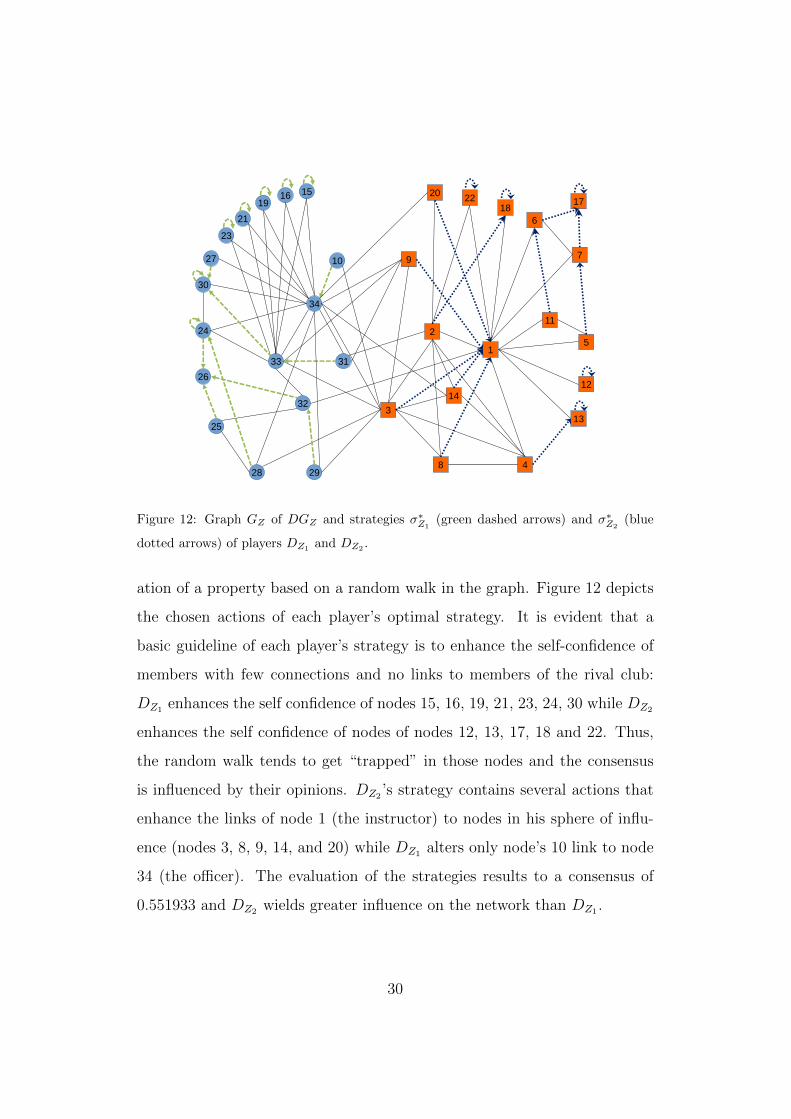
Figure 12: Graph GZ of DGZ and strategies σ∗Z1(green dashed arrows) and σ∗Z2

(blue

dotted arrows) of players DZ1and DZ2

.

ation of a property based on a random walk in the graph. Figure 12 depicts

the chosen actions of each player’s optimal strategy. It is evident that a

basic guideline of each player’s strategy is to enhance the self-confidence of

members with few connections and no links to members of the rival club:

DZ1 enhances the self confidence of nodes 15, 16, 19, 21, 23, 24, 30 while DZ2

enhances the self confidence of nodes of nodes 12, 13, 17, 18 and 22. Thus,

the random walk tends to get “trapped” in those nodes and the consensus

is influenced by their opinions. DZ2 ’s strategy contains several actions that

enhance the links of node 1 (the instructor) to nodes in his sphere of influ-

ence (nodes 3, 8, 9, 14, and 20) while DZ1 alters only node’s 10 link to node

34 (the officer). The evaluation of the strategies results to a consensus of

0.551933 and DZ2 wields greater influence on the network than DZ1 .

30

0

200

400

600

800

1.000

1.200

1.400

1.600

10 20 30 40 50 60 70 80 90 100

0

5

10

15

20

25

10 20 30 40 50 60 70 80 90 100

Figure 13: PRISM’s execution times of (a): DP and DIP experiments, (b): DG experi-

ments.

5.7. Measurements of model checking times and other solution techniques

In order to examine the computational demands of our models and com-

pare their efficiency with other solution techniques, we developed a bench-

mark suite consisting of auto-generated scale-free graphs of various sizes and

measured the algorithms’ execution times. The experiments were conducted

on an Intel R© CoreTM i7-4770K CPU @ 3.50GHz workstation with 11GB of

system memory, running Ubuntu 16.04.3 LTS. The installed Java platform

was Oracle JDK 8u161, whereas the results were obtained using PRISM ver-

sion 4.4 and PRISM-games version 2.0.beta3. PRISM’s and PRISM-games’

explicit engine was utilized for the evaluation of properties in the cases of

DP , DIP and DG while the sparse engine computed the Pareto sets of the

CDIP models.

The benchmark suite consisted of ten classes of DP , DIP and DG models

with different graph sizes (10, 20,..., 90, 100 nodes). Figure 13 illustrates the

average execution times observed for each category. For the DP experiments,

the reported times include the building of the model and the evaluation of

consensus b∗c of the graph. They clearly exhibit a linear scaling behaviour

and even for large models the solution is rapidly computed (the average time

for a graph with 100 nodes is 0.20516 seconds). For the DIP experiments,

31

0

200

400

600

800

1.000

1.200

1.400

1.600

1.800

6 7 8 9 10 11 12 13 14

Figure 14: PRISM’s execution times of CDIP experiments

our measurements reveal an evident yet affordable increase in the complex-

ity of calculations (the average time for a graph with 100 nodes is 20.5919

seconds). For the DG experiments, the reported times include the building

of the model and the evaluation of the final consensus. The results indicate a

significant complexity increase compared to the DP and DIP measurements

(the average time for a graph with 100 nodes is 1519.673 seconds).

The benchmark suite contains nine classes of CDIP models with fewer

nodes (6, 7,..., 13, 14 nodes), due to the longer duration of computations

even for graphs with much smaller size. Figure 14 illustrates the average

execution times for Pareto curve generation that clearly demands more time

and resource allocation compared to the experiments of DP and DIP . For

example, the average time for ten-node graphs is 195.305 seconds, while the

corresponding time for the DIP of Figure 13 takes 0.5227 seconds. The aver-

age execution time for the CDIP in fifteen-node graphs is 670.7168 seconds.

Previous experiments on the extraction of Pareto curves [31] with PRISM’s

sparse engine provided evidence of polynomial complexity in similar experi-

ments, and our results abide with this conclusion.

For the DP and DIP problems it was possible to compute the consensus

32

and the optimal strategy for the decision maker, using GNU Octave ver-

sion 4.0.0, a prominent mathematical solver, together with its toolbox for

MDPs [8]. However, no adequate support was found by Octave, for the anal-

ysis of the CDIP and DG problems. With a similar series of experiments,

whose solution times are shown in Figure 15, we found that Octave outper-

forms our model checking approach in PRISM. For graphs with 100 nodes,

the average time for the DP models using PRISM is 0.20516 sec, while in

Octave the corresponding time is 0.00307 sec. For the extraction of the de-

cision maker’s strategy in our DIP models of social graphs with 100 nodes,

our model checking approach lasts in average 20.5919 sec, while in Octave it

lasts merely 0.00963 sec.

These experiments show that the mathematical solver is more properly

equipped and, therefore, more efficient for the analysis of DP and DIP mod-

els. Specifically for the DIP , this finding is attributed to the used toolbox,

which includes specialized functions for extracting the optimal strategy in an

MDP. Such a functionality is not provided directly in PRISM, which forced

us to resort to an elaborate formulation of the problem using random walks.

This approach eventually resulted in an increased overhead in our solution

times measurements.

On the other hand, PRISM’s high-level modelling language offers a more

human-friendly environment for the model formulation. In Octave, for the

same model it is necessary to define multi-dimensional numerical matrices

that is overly bewildering.

For the CDIP problem, we are not aware of any other integrated analysis

environment with support for the formulation of the model and the evaluation

of Pareto curves. The available functionality and expressiveness of PRISM’s

property language offer a significant advantage for the analysis of CDIP

33

0

5

10

15

20

25

10 20 30 40 50 60 70 80 90 100

0,00

0,05

0,10

0,15

0,20

0,25

0,30

10 20 30 40 50 60 70 80 90 100

Figure 15: Execution times of: (a) DP experiments, (b) DIP experiments

models.

The analysis of the DG problem in a mathematical environment like

Octave can be achieved only by the use of a brute force algorithm. For

this purpose, we automated the process of suitably transcribing the DG

experiments for Octave and measured the times for graphs of 10 nodes. The

average time using Octave is 683.31 sec, while the analysis with PRISM-

games requires in average 39.57 sec. For larger models in Octave, the process

did not terminate in a reasonable time period. This is justified by the fact

that the addition of nodes in the graph leads to an exponential increase in

the number of alternatives to be checked by the brute force algorithm.

6. Discussion

The rapid growth of social networks and their impact on the formation

of social consensus call for deeper research on the opinion diffusion process.

The DeGroot learning model is a simple yet efficient procedure that simulates

opinion dynamics and incorporates elaborate characteristics of the process.

In [10], we introduced three classes of models (DP , DIP and CDIP ) that

incorporate the DeGroot model into social networks. We proposed proba-

bilistic model checking techniques, adequate for efficiently formulating the

DeGroot opinion diffusion process and we provided the means to analyze the

34

model, when strategic entities aim to interfere with the consensus formation.

Preliminary experimental results indicated that PRISM is adequate in terms

of solution times for the task of optimal strategy construction, when external

intervention is applied.

In current work, a new model class (CDIP ) is introduced that demon-

strates the trade-off between influence in a social network and cost, for the

decision maker. PRISM allow to easily model the CDIP problem and evalu-

ate its Pareto curves; to the best of our knowledge, the popular mathematical

solvers lack support for formulating the CDIP problem.

Further experimentation revealed the range of influence that can be wielded

on a social network by the strategic players, for various sets of possible ac-

tions. In the case of one strategic entity, the impact of entity’s intervention

attenuates as the strength of his actions increases, which indicates the limits

of influence that can be wielded in the consensus formation. When having

two competitive strategic entities, their strategies tend to nullify each other

and, hence, any observable alteration in the consensus can be attributed to

the structural characteristics of the social network that may enhance slightly

the impact of one player.

The experiments unveiled the advantages and disadvantages of our model

checking approach compared to existing mathematical solvers. The latter

outperform PRISM, when analysing simple scenarios of opinion diffusion and

intervention, such as the DP and DIP , while for more elaborate scenarios,

such as CDIP and DG, the solvers do not provide the means to formulate

and analyze the models. The remaining alternative, i.e., brute force analysis,

exhibits worse performance in small-scale models than model checking and

cannot tackle the analysis of larger models.

The application of the proposed models on a prominent case study of real

35

life social networks, the Zachary’s karate club, illustrates their use on small

but more realistic graphs. The results highlight various aspects of strategic

intervention in real life social graphs and provide solid ground for future work

on other real graph-structured applications (e.g., social media).

Finally, our research unveils the computational aspects of modeling De-

Groot influence problems as stochastic processes. More specifically, the for-

mulation of a DeGroot model as Markov chain for the DP and as MDP for

the DIP and CDIP can be effectively accomplished, while in the case of

DG, the solution of the stochastic game exhibits a considerable increase of

complexity, due to the multiple alternatives offered to the players.

References

[1] M. H. DeGroot, Reaching a consensus, Journal of the American Statis-

tical Association 69 (345) (1974) 118–121.

[2] N. E. Friedkin, E. C. Johnsen, Social influence and opinions, Journal of

Mathematical Sociology 15 (3-4) (1990) 193–206.

[3] N. E. Friedkin, E. C. Johnsen, Social influence networks and opinion

change, Advances in group processes 16 (1) (1999) 1–29.

[4] R. Hegselmann, U. Krause, et al., Opinion dynamics and bounded con-

fidence models, analysis, and simulation, Journal of artificial societies

and social simulation 5 (3) (2002) 1–24.

[5] M. Kwiatkowska, G. Norman, D. Parker, PRISM 4.0: Verification of

Probabilistic Real-time Systems, in: CAV’11, LNCS 6806, Springer,

2011, pp. 585–591.

36

[6] S. A. W. Cordwell, pymdptoolbox 4.0-b3, https://pypi.python.org/

pypi/pymdptoolbox/ (Jan. 2015).

[7] T. Chen, V. Forejt, M. Kwiatkowska, D. Parker, A. Simaitis, PRISM-

games: A Model Checker for Stochastic Multi-Player Games, in:

N. Piterman, S. Smolka (Eds.), Proc. 19th International Conference on

Tools and Algorithms for the Construction and Analysis of Systems

(TACAS’13), Vol. 7795 of LNCS, Springer, 2013, pp. 185–191.

[8] M.-J. Cros, Markov Decision Processes (MDP) Toolbox,

http://www.mathworks.com/matlabcentral/fileexchange/25786-

markov-decision-processes--mdp--toolbox (Nov. 2009).

[9] M. Kwiatkowska, G. Norman, D. Parker, Stochastic Model Checking,

in: M. Bernardo, J. Hillston (Eds.), Formal Methods for the Design of

Computer, Communication and Software Systems: Performance Evalu-

ation (SFM’07), Vol. 4486 of LNCS (Tutorial Volume), Springer, 2007,

pp. 220–270.

[10] S. Gyftopoulos, P. S. Efraimidis, P. Katsaros, Solving Influence Prob-

lems on the DeGroot Model with a Probabilistic Model Checking Tool,

in: Proceedings of the 20th Pan-Hellenic Conference on Informatics,

ACM, 2016, p. 31.

[11] W. W. Zachary, An information flow model for conflict and fission in

small groups, Journal of anthropological research 33 (4) (1977) 452–473.

[12] T. L. Tuten, M. R. Solomon, Social media marketing, Sage, 2014.

[13] D. Zarrella, The social media marketing book, O’Reilly Media, Inc.,

2009.

37

[14] W. G. Mangold, D. J. Faulds, Social media: The new hybrid element of

the promotion mix, Business horizons 52 (4) (2009) 357–365.

[15] R. W. Naylor, C. P. Lamberton, P. M. West, Beyond the like button:

The impact of mere virtual presence on brand evaluations and purchase

intentions in social media settings, Journal of Marketing 76 (6) (2012)

105–120.

[16] M. R. Sciandra, C. Lamberton, R. W. Reczek, The Wisdom of Some:

Do We Always Need High Consensus to Shape Consumer Behavior?,

Journal of Public Policy & Marketing 36 (1) (2017) 15–35.

[17] J. Castro, J. Lu, G. Zhang, Y. Dong, L. Mart́ınez, Opinion

Dynamics-Based Group Recommender Systems, IEEE Transactions

on Systems, Man, and Cybernetics: Systems PP (99) (2017) 1–13.

doi:10.1109/TSMC.2017.2695158.

[18] U. Krause, A discrete nonlinear and non-autonomous model of consensus

formation, Communications in difference equations 2000 (2000) 227–236.

[19] Y. Yu, G. Xiao, G. Li, W. P. Tay, Opinion diversity and community

formation in adaptive networks (Mar. 2017). arXiv:1703.02223.

[20] P. Holme, M. E. Newman, Nonequilibrium phase transition in the co-

evolution of networks and opinions, Physical Review E 74 (5) (2006)

056108.

[21] R. Basu, A. Sly, et al., Evolving voter model on dense random graphs,

The Annals of Applied Probability 27 (2) (2017) 1235–1288.

[22] G. Deffuant, D. Neau, F. Amblard, G. Weisbuch, Mixing beliefs among

interacting agents, Advances in Complex Systems 3 (2000) 87–98.

38

[23] X. Meng, R. A. Van Gorder, M. A. Porter, Opinion formation and distri-

bution in a bounded confidence model on various networks (Jan. 2017).

arXiv:1701.02070.

[24] S. Huang, Probabilistic model checking of disease spread and prevention,

in: Scholarly Paper for the Degree of Masters in University of Maryland,

2009.

[25] L. Dennis, M. Slavkovik, M. Fisher, ‘How Did They Know?’ - Model-

checking for Analysis of Information Leakage in Social Networks, in:

Joint post-proceedings of the COIN@AAMAS 2016 and COIN@ECAI

2016 workshops, Lecture Notes in Computer Science, Springer, 2017.

[26] L. S. Shapley, Stochastic games, Proceedings of the National Academy

of Sciences 39 (10) (1953) 1095–1100.

[27] T. Bewley, E. Kohlberg, The asymptotic theory of stochastic games,

Mathematics of Operations Research 1 (3) (1976) 197–208.

[28] R. Bellman, A Markovian decision process, Journal of Mathematics and

Mechanics (1957) 679–684.

[29] R. A. Howard, Dynamic programming and Markov processes, Technol-

ogy Press of Massachusetts Institute of Technology, 1960.

[30] M. Kwiatkowska, D. Parker, C. Wiltsche, PRISM-games 2.0: A

Tool for Multi-Objective Strategy Synthesis for Stochastic Games, in:

M. Chechik, J.-F. Raskin (Eds.), Proc. 22nd International Conference

on Tools and Algorithms for the Construction and Analysis of Systems

(TACAS’16), Vol. 9636 of LNCS, Springer, 2016, pp. 560–566.

39

[31] V. Forejt, M. Kwiatkowska, D. Parker, Pareto Curves for Probabilistic

Model Checking, in: S. Chakraborty, M. Mukund (Eds.), Proc. 10th

International Symposium on Automated Technology for Verification and

Analysis (ATVA’12), Vol. 7561 of LNCS, Springer, 2012, pp. 317–332.

[32] M. O. Jackson, Social and Economic Networks, Princeton University

Press, 2008.

[33] M. Bianchini, M. Gori, F. Scarselli, Inside pagerank, ACM Transactions

on Internet Technology (TOIT) 5 (1) (2005) 92–128.

[34] L. Page, S. Brin, R. Motwani, T. Winograd, The PageRank Citation

Ranking: Bringing Order to the Web., Technical Report 1999-66, Stan-

ford InfoLab (November 1999).

[35] L. R. Ford Jr, D. R. Fulkerson, Flows in networks, Princeton university

press, 2015.

[36] T. Quatmann, J.-P. Katoen, Sound value iteration, in: H. Chockler,

G. Weissenbacher (Eds.), Computer Aided Verification, Springer Inter-

national Publishing, Cham, 2018, pp. 643–661.

[37] A. Simaitis, Automatic verification of competitive stochastic systems,

Ph.D. thesis, University of Oxford (2014).

[38] A. Condon, The complexity of stochastic games, Information and Com-

putation 96 (2) (1992) 203–224.

[39] T. Deshpande, P. Katsaros, S. A. Smolka, S. D. Stoller, Stochastic

Game-Based Analysis of the DNS Bandwidth Amplification Attack Us-

ing Probabilistic Model Checking, in: Dependable Computing Conf.,

2014 Tenth European, IEEE, 2014, pp. 226–237.

40

[40] L. Kallenberg, Finite state and action mdps, in: Handbook of Markov

decision processes, Springer, 2003, pp. 21–87.

[41] E. A. Feinberg, A. Shwartz, Handbook of Markov decision processes:

methods and applications, Vol. 40, Springer Science & Business Media,

2012.

[42] K.-J. Bierth, An expected average reward criterion, Stochastic processes

and their applications 26 (1987) 123–140.

Appendix A. Proof of Proposition 1

We consider a Markov Decision Process (MDP) as described by Kallen-

berg in [40]. The MDP is defined as a discrete, finite Markovian decision

problem with finite state space X and finite action sets A(i), i ∈ X. The

decision times t are equidistant, say t = 1, 2, .... When the process is at state

i and action a ∈ A(i) is chosen, a reward r(i, a) is assigned immediately and

the process moves to state j ∈ X with transition probability p(j | i, a), where

∀j, i, a, p(j | i, a) ≥ 0, and ∀i, a,∑

j p(j | i, a) = 1. A stationary policy π is

defined as a mapping π : X→ A such that π(i) ∈ A(i) for all i ∈ X and ΠS

is the set of all stationary policies [41]. By definition, a stationary policy is

independent of decision time t, i.e., action π(i) is the same regardless of the

decision time t that state i occurs.

The performance of a MDP under a policy is expressed using a utility

function. This function can be the expected total reward of the MDP over a

planning horizon or the average expected reward per time unit [40]. Suppose

that the MDP is controlled over a finite planning horizon T . Let X × A =

{(i, a) | i ∈ X, a ∈ A} and random variables Xt and Yt denote the state and

41

action at time t of T . Then, the lower limit of the average expected reward

of MDP under a policy π starting from state i is defined as:

ϕ(i, π) := lim infT→∞

1

T

T∑t=1

Ei,π [r(Xt, Yt)] , i ∈ X

Bierth [42] has shown that there exists a stationary strategy which is

optimal for the lower limit of the average expected reward. Therefore:

∃π∗ ∈ ΠS,∀π ∈ ΠS,∀i ∈ X, ϕ(i, π∗) ≤ ϕ(i, π)⇒

lim infT→∞

1

T

T∑t=1

Ei,π∗ [r(Xt, Yt)] ≤ lim infT→∞

1

T

T∑t=1

Ei,π [r(Xt, Yt)]

We can safely deduce that there exists a tL such that:

∀t ∈ N, t > tL,1

t

t∑t=1

Ei,π∗ [r(Xt, Yt)] ≤1

t

t∑t=1

Ei,π [r(Xt, Yt)]

t∑t=1

Ei,π∗ [r(Xt, Yt)] ≤t∑t=1

Ei,π [r(Xt, Yt)]

The summations of the last equation express the total expected reward of

the MDP over a planning horizon of length t. Therefore, policy π∗ minimizes

also the total expected reward of the MDP for planning horizons with length

greater than a limit tL.

42