Notes for Chapter 1 of DeGroot and Schervish1 The world is full of random events that we seek to understand. Ex. `Will it snow tomorrow?'

`What are our chances of winning the lottery?' ‘What is the time between emission of alpha particles by a radioactive source?’

The outcome of these questions cannot be exactly predicted in advance. But the occurrence of these phenomena is not completely haphazard. The outcome is uncertain, but there is a regular pattern to the outcome of these random phenomena.

Ex. If I flip a fair coin, I do not know in advance whether the result will be a head or tail, but I can say in the long run approximately half the time the result will be heads.

Probability theory is a mathematical representation of random phenomena. A probability is a numerical measurement of uncertainty. Applications:

• Quantum mechanics • Genetics • Finance • Computer science (analyze the performance of computer algorithms that employ

randomization) • Actuarial science (computing insurance risks and premiums) • Provides the foundation for the study of statistics.

The theory of probability is often attributed to the French mathematicians Pascal and Fermat (~1650). Began by trying to understand games of chance. Gambling was popular. As the games became more complicated and the stakes increased, there was a need for mathematical methods for computing chance.

1 These notes adapted from Martin Lindquist’s notes for STAT W4105 (Probability).

Through history there have been a variety of different definitions of probability. Classical Definition: Suppose a game has n equally likely outcomes of which m outcomes (m<n) correspond to winning. Then the probability of winning is m/n. Ex. A box contains 4 blue balls and 6 red balls. If I randomly pick a ball from the box, what is the probability it is blue? n=10, m=4, P(blue ball) = 4/10 = 2/5. The classical definition requires a game to be broken down into equally likely outcomes. Ideal situation with very limited scope. Relative Frequency Definition: Repeat a game a large number of times under the same conditions. The probability of winning is approximately equal to the number of wins in the repeated trials. Ex. Flip a coin 100,000 times. We get approximately 50,000 heads. P(Heads) = ½. Frequency approach is consistent with the classical approach. Subjective probability is a degree of belief in a proposition. Axiomatic Approach: Kolmogorov developed the first rigorous approach to probability (~1930). He built up probability theory from a few fundamental axioms. The book and this course will use these axioms to build up the theory of probability. Modern research in probability is closely related to measure theory. This course avoids most of these issues and stresses intuition.

Sample Space and Events One of the main objectives of statistics and probability theory is to draw conclusions about a population of objects by conducting an experiment. We must begin by identifying the possible outcomes of an experiment, or the sample space. Definition: The set, S, of all possible outcomes from a random experiment is called the sample space. Ex. Flip a coin. Two possible outcomes: Heads (H) or Tails (T). Thus, S={H, T}. Ex. Roll a die. Six possible outcomes: S={1, 2, 3, 4, 5, 6}. Ex. Roll two dice. 36 possible outcomes: S={(i,j) | i=1,….6, j=1,….6 }. Ex. Lifetime of a battery. S = {x: 0 ≤x<∞} Definition: An event is any collection of possible outcomes of an experiment, that is, any subset of S (including S itself). If the outcome of the experiment is contained in an event E, then we say that E has occurred. Ex. Flip two coins. Four possible outcomes: HH, HT, TH, TT. Thus, S={HH, HT, TH, TT}. An event could be obtaining at least one H in the two tosses. Thus, E={HH, HT, TH}. Note E does not contain TT. Ex. Battery example. E = {x: x<3} (The battery lasts less than 3 hours.)

Set Theory Given any two events (or sets) A and B, we have the following elementary set operations: Union: The union of A and B, written A∪B, is the set of elements that belong to either A or B or both: A∪B = {x:| x∈A or x∈B} If A and B are events in an experiment with sample space S, then the union of A and B is the event that occurs if and only if A occurs or B occurs. Venn diagram – The sample space is all the outcomes in a large rectangle. The events are represented as consisting of all the outcomes in given circles within the rectangle. Intersection: The intersection of A and B, written A∩B or AB, is the set of elements that belong to both A and B: AB = {x:| x∈A and x∈B} If A and B are events in an experiment with sample space S, then the intersection of A and B is the event that occurs if and only if A occurs and B occurs Complementation: The complement of A, written AC, is the set of all elements that are not in A: AC = {x:| x∉A } If A is an event in an experiment with sample space S, then the complement of A is the event that occurs if and only if A does not occur. Ex. Select a card at random from a standard deck of cards, and note its suit: clubs (C), diamonds (D), hearts (H) or spades (Sp). The sample space is S={C,D,H,Sp}. Some possible events are A={C,D}, B={D,H,Sp} and C={H}. A∪B ={C,D,H,Sp} = S AB ={D} AC ={H,Sp} AC = ∅ (null event – event consisting of no outcomes)

If AB =∅ then A and B are said to be mutually exclusive. For any two events A and B, if all of the outcomes in A are also in B, then we say that A is contained in B. This is written A⊂B. Ex. Roll a fair die. S = {1,2,3,4,5,6} Let E={1,3,5} and F={1}, then F⊂E. Note that if A⊂B then the occurrence of A implies the occurrence of B. Also if A⊂B and B⊂A then A=B. The operations of forming unions, intersections and complements of events follow certain basic laws. Basic laws Commutative Laws: E∪F= F∪E

EF=FE Associative Laws: (E∪F) ∪G = E∪(F∪G)

(EF)G=E(FG) Distributive Laws: (E∪F) G = EG∪FG

(EF) ∪G=(E∪G)(F∪G) DeMorgan’s Laws (A∪B)C=ACBC (*) (AB)C=AC∪BC

Proof of (*): x ∈ (A∪B)C ⇒ x ∉ A∪B ⇒ x ∉ A and x ∉ B ⇒ x ∈ AC and x ∈ BC ⇒ x ∈ ACBC Hence, (A∪B)C ⊂ ACBC x ∈ ACBC ⇒ x ∈ AC and x ∈ BC ⇒ x ∉ A and x ∉ B ⇒ x ∉ A∪B ⇒ x ∈ (A∪B)C Hence, ACBC ⊂ (A∪B)C Since (A∪B)C ⊂ ACBC and ACBC ⊂ (A∪B)C , it must hold that ACBC = (A∪B)C The proofs of the other laws are done in a similar manner. Often we are interested in unions and intersections of more than two events. Definition: { | for atleast one }

i i

i I

A x x A i I

!

= ! !U

and { | for every }

i i

i I

A x x A i I

!

= ! !I

Generalized DeMorgan’s Laws:

(a) ( )

C

C

i i

i I i I

A A

! !

" #=$ %

& 'U I

(b) ( )

C

C

i i

i I i I

A A

! !

" #=$ %

& 'I U

Axioms of Probability Consider an experiment whose sample space is S. For each event E of the sample space S we assume that a number P(E) is defined and satisfies the following three axioms. Axiom 1: 0 <= P(E) <= 1 Axiom 2: P(S) =1 Axiom 3: For any sequence of mutually exclusive events E1, E2, …… ,

11

( )i i

ii

P E P E

! !

==

" #=$ %

& '(U .

We refer to P(E) as the probability of the event E. Ex. For any finite sequence of mutually exclusive events E1, E2, ….. En,

11

( )n n

i i

ii

P E P E

==

! "=# $

% &'U

Proposition 1: P(EC) = 1-P(E) Proof: E and EC are mutually exclusive and S=E∪EC. By Axiom 2: P(S) = 1 By Axiom 3: P(S) = P(E∪EC) = P(E) + P(EC) Hence, P(EC) = 1 - P(E) Ex. Let E=S. Then EC=∅. P(∅) = 1- P(S) = 1-1 = 0

Ex. Roll a fair dice 3 times. What is the probability of at least one six, if we know that the probability of getting 0 sixes is 0.579? P(at least one six) = 1- P(0 sixes) 1- 0.579 = 0.421 Proposition 2: If E⊂F, then P(E) <= P(F). Proof: Since E⊂F, F= E∪ECF. E and ECF are mutually exclusive, Axiom 3 gives P(F) = P(E) + P(ECF). But P(ECF)>=0 by Axiom 1. Hence, P(F) >= P(E) Proposition 3: P(E∪F) = P(E) + P(F) – P(EF) Proof: E∪F = E∪ECF E and ECF are mutually exclusive. P(E∪F) = P(E∪ECF) = P(E) + P(ECF) ⇒ P(ECF) = P(E∪F) – P(E) F = EF∪ECF EF and ECF are mutually exclusive. P(F) = P(EF∪ECF) = P(EF) + P(ECF) ⇒ P(ECF) = P(F) – P(EF) Together, P(F) – P(EF) = P(E∪F) – P(E)

⇒ P(E∪F) = P(E) + P(F) – P(EF) Ex. A store accepts either VISA or Mastercard. 50% of the stores customers have VISA, 30% have Mastercard and 10% have both.

(a) What percent of the stores customers have a credit card the store accepts? A = customer has VISA B = customer has Mastercard P(A∪B) = P(A) + P(B) – P(AB) = 0.50 + 0.30 – 0.10 = 0.70 (b) What percent of the stores customers have exactly one of the credit cards the

store accepts?

P(A∪B) – P(AB) = 0.70 –0.10 = 0.60 (c) What percent of the stores customers doesn’t have a credit card the store accepts? P(0 cards) = 1-P(at least one card) = 1- 0.70 = 0.30

Proposition 4:

1 2 1 2

1 2 1 2

1 2

1 2

1

1 2

1

1

( ) ( ) ( ) ( 1) ( )

( 1) ( )

r

r

n

n

n

r

i i i i i i

i i i i i i

n

i i i

i i i

P E E En P E P E E P E E E

P E E E

+

= < < < <

+

< < <

! ! ! = " + + "

+ + "

# # #

#L

L

L K L

L L

The summation

1 2

1 2

( )r

r

i i i

i i i

P E E E

< < <

!L

L is taken over all (n r) possible subsets of size r of

the set {1,2,…,n}. Ex. Three events E, F and G. P(E∪F∪G) = P(E) + P(F) + P(G) – P(EF) – P(EG) – P(FG) + P(EFG)

Combinatorial Analysis Many problems in probability theory can be solved by simply, counting the number of different ways an event can occur. The mathematical theory of counting is formally known as combinatorial analysis The Sum Rule: If a first task can be done in m ways and a second task in n ways, and if these tasks cannot be done at the same time, then there are m + n ways to do either task Ex. A library has 10 textbooks dealing with statistics and 15 textbooks dealing with biology. How many textbooks can a student choose from if he is interested in learning about either statistics or biology? 10+15 = 25 Ex. At a cafe one can choose between three different snacks: ice cream, cake or pie. Additionally there are two different beverages: coffee or tea. How many possible combinations are there if we are allowed to choose one snack and one beverage? Tree diagram: IC, IT; CakeC, CakeT; PC,PT 6 different possible combinations. Basic principle of counting: If two successive choices are to be made with m choices in the first stage and n choices in the second stage, then the total number of successive choices is n*m. (This is sometimes referred to as the product rule.) Proof: We can write the two choices as (i,j), if the first choice is i and the second j. i=1,……m and j=1,…….n Enumerate all the possible choices: (1,1), (1,2), …… (1,n) (2,1), (2,2), …… (2,n) : : (m,1), (m,2), …… (m,n) The set of possible choices consists of m rows, each row consisting of n elements.

Hence m*n total choices. -- The generalized basic principle of counting: If r successive choices are to be made with exactly nj choices at each stage, then the total number of successive choices is n1*n2*…..*nr Ex. A license plate consists of 3 letters followed by 2 numbers. How many possible license plates are there? 26*26*26*10*10=1,757,600 What if repetitions of letters and numbers are not allowed? 26*25*24*10*9=1,404,000

Permutations An ordered arrangement of the objects in a set is called a permutation of the set. Ex. How many ways can we rank three people: A, B and C? ABC, ACB, BAC, BCA, CAB, CBA Each arrangement is called a permutation. There are 6 different permutations in this case. _ _ _

We use the BPC to describe our selection. We have three letters to choose from in filling the first position, two letters remain to fill the second position, and just one letter left for the last position: 3x2x1=6 different orders are possible. Another way of writing this is 3!.

Definition: For an integer n>=0, n! = n(n-1)(n-2) …..3*2*1

0! =1 Note that n! = n(n-1)! The number of different permutations of n distinct objects is n(n-1)…..1=n! Ex. How many different letter arrangements can be made of the word COLUMBIA. Ans. 8! Ex. How many ways can we choose a President, Vice-President and Secretary from a group consisting of five people? President can be chosen 5 different ways Vice-President can be chosen 4 different ways, Secretary can be chosen 3 different ways 5*4*3=120 The number of different permutations of r objects taken from n distinct objects is n(n-

1)….(n-r+1).

Note: n(n-1)….(n-r+1) = n!/(n-r)! Ex. How many ways can we choose a President, Vice-President and Secretary from a group consisting of five people if A will only serve if he is President? A serves 1*4*3=12

OR A doesn’t serve 4*3*2=24 Total = 12+24 = 36 Finally, what is the number of permutations of a set of n objects when certain objects are indistinguishable from one another? Ex. How many permutations of the letters in the set {M,O,M} can we make? There are 3! different ways to arrange a three letter word, when all the letters are different. But in this case the two M’s are indistinguishable from one another. Order the objects as if they were distinguishable. Rewrite as (M1,O,M2) 3! different ways to arrange these three letters. M1OM2, M1M2O, OM1M2, OM2M1, M2OM1, M2M1O But M1OM2 is the same as M2OM1 when the subscripts are removed. We need to compensate for this. How many ways can we arrange the 2 M’s in the two slots. (2!) Divide out the arrangements that look identical. 3!/2!=3 distinct arrangements. In general there are n!/n1!-------nr! different permutations of n objects, of which n1 are

alike, n2 are alike, etc…..

Ex. How many different letter arrangements can be made from the letters MISSISSIPPI?

1 M, 4 I’s, 4 S’s, 2 P’s (11!/(1!4!4!2!) = 34,650

Combinations A permutation is an ordered arrangement of r objects from a set of n objects. Ex. How many ways can we choose a President, Vice-President and Secretary from a group consisting of five people? President can be chosen 5 different ways Vice- President can be chosen 4 different ways, Secretary can be chosen 3 different ways 5!/2! A Combination is an unordered arrangement of r objects from a set of n objects. Ex. Suppose instead of picking a President, Vice-President and Secretary we would just like to pick three people out of the group of five to be on the leadership board, i.e. how many teams of three can we create from a larger group consisting of five people? In this case order does not matter. Each combination of three people is counted 3! times. We need to compensate for this. 5!/(2!3!) When counting permutations abc and cab are different. When counting combinations they are the same. Notation: n choose r (n r) = n!/(n-r)!r! for 0<=r<=n. (n r) represent the number of ways we can choose groups of size r from a larger group of size n, when the order of selection is not relevant. SHOW AT HOME: Property 1: (n r) = (n (n-r)). Property 2: (n r) = ((n-1) r) + ((n-1) (r-1)). Ex. How many ways can I choose 5 cards from a deck of 52. (52 5) =2,598,960 (Total number of poker hands)

Ex. (Q.20 p.17) A person has 8 friends, of whom 5 will be invited to a party.

(a) How many choices are there if 2 of the friends are feuding and will not attend together?

(b) How many choices if 2 of the friends will only attend together?

(a) One of the feuding friends attends and the other does not. (2 1)(6 4) or

Neither of the feuding friends attend. (6 5) Total = 2*15+6 = 36

(b) The two friends attend together. (6 3) = 20 or The two friends do not attend. (6 5) = 6 Total = 20+6 = 26

Ex. A committee of 6 people is to be chosen from a group consisting of 7 men and 8 women. If the committee must consist of at least 3 women and at least 2 men, how many different committees are possible?

3 women/ 3 men: (8 3)*(7 3) or 4 women/ 2 men: (8 4)*(7 2)

Total = (8 3)*(7 3) + (8 4)*(7 2) = 3430.

The symbol (n r) is sometimes called a binomial coefficient.

The binomial theorem If x and y are variables and n is a positive integer, then

(x+y)^n = sum_{k=0}^{n} (n k) x^k y^(n-k) Ex. (x+y)^2 = (2 0) x^0y^2 + (2 1) x^1y^1 + (2 2) x^2y^0 = y^2 + 2xy + x^2 Ex. Prove that sum_{k=0}^{n} (n k) = 2^n. Set x=1 and y=1. By binomial theorem (1+1)^n = sum_{k=0}^{n} (n k) 1^k 1^(n-k) 2^n = sum_{k=0}^{n} (n k) Multinomial Coefficients Ex. How many ways are there of assigning 10 police officers to 3 different tasks, if 5 must be on patrol, 2 in the office and 3 on reserve? (10 5) (5 2) (3 3) = 10!/(5!2!3!) In general there will n!/(n1!n2!…nr!) ways to divide up n objects into r different categories so that there will be n1 objects in category 1, n2 in category 2, and so on, where (n1+…nr=n). Notation: If n1+n2+…+nr=n, we define (n n1,n2,….nr) = n!/(n1!….nr!) The symbol (n n1,n2,…nr) is sometimes called a multinomial coefficient. The multinomial theorem (x1+x2+……+xr)^n = sum_{(n1,…….,nr): n1+….+nr=n} (n n1,n2,….nr) x1^n1 x2^n2 … xr^nr That is, the sum is over all nonnegative integer-valued vectors (n1, …….,nr) such that n1+….+nr=n.

Sample Spaces having equally likely outcomes The assignment of probabilities to sample points can be derived from the physical set-up of an experiment. Consider the scenario that we have N sample points, each equally likely to occur. Then each has a probability of 1/N. Example: a fair coin, a fair dice or a poker hand. Assume an event consisting of M sample points. The probability of the event occurring is M/N. Ex. Flip two fair coins. S = {HH, HT, TH, TT}. Our sample space consists of 4 points, each of which is equally likely to occur. P(HH) = 1/4. Let E= at least one head = {HH, HT, TH}. P(E) = ¾. Let F= exactly one head = {HT, TH}. P(E) = 2/4 = 1/2. Ex. Roll two dice. S={(i,j) | i=1,….6, j=1,….6 } There are 36 possible outcomes. What is the probability that the total of the two dice is less than or equal to 3? E = sum of the two dice are less than or equal to 3. (1,1), (1,2), (2,1) P(E) = 3/36 = 1/12. Ex. Two cards are chosen at random from a deck of 52 playing cards. What is the probability that they (a) are both aces? (b) are both spades?

(a) Total number of ways to choose two cards - (52 2) Total number of ways to choose two aces - (4 2)

P(two aces) = (4 2)/(52 2) = 1/221 (b) Total number of ways to choose two cards - (52 2) Total number of ways to choose two spades - (13 2) P(two spades) = (13 2)/(52 2) = 1/17

Ex. Poker hands. Choose a five-card poker hand from a standard deck of 52 playing cards. What is the probability of four aces? There are (52 5) = 2,598,960 possible hands. Having specified that four cards are aces, there are 48 different ways of specifying the fifth card. P(four aces) = 48/2,598,960. What is the probability of a full house (one 3 of a kind + one pair)? There are 13 ways to pick ways to choose the denomination of the three of a kind. There are (4 3) different ways to choose three cards of that denomination. There are 12 ways to pick ways to choose the denomination of the pair. There are (4 2) different ways to choose two cards of that denomination. P(full house) = 13*(4 3)*12*(4 2)/(52 5) = 3,744/2,598,960

Suppose you flip a coin and bet that it will come up tails. Since you are equally likely to get heads or tails, the probability of tails is 50%. This means that if you try this bet often, you should win about half the time. What if somebody offered to bet that at least two people in your math class had the same birthday? Would you take the bet? Ex. The Birthday Problem. What is the probability that at least two people in this class share the same birthday? Assumptions: • 365 days in a year. (No leap year). • Each day of the year has an equal chance of being somebodies birthday

(Birthdays are evenly distributed over the year). E = no two people share a birthday. EC = at least two people share a birthday. Use Proposition 1 from last time: P(at least two people share birthday) = 1 - P(no two people share birthday). What is the probability that no two people will share a birthday? The first person can have any birthday. The second person's birthday has to be different. There are 364 different days to choose from, so the chance that two people have different birthdays is 364/365. That leaves 363 birthdays out of 365 open for the third person. To find the probability that both the second person and the third person will have different birthdays, we have to multiply: (365/365) * (364/365) * (363/365) = 0.9918. If we want to know the probability that four people will all have different birthdays, we multiply again: (365/365) *(364/365) * (363/365) * (362/365) = 0.9836. We can keep on going the same way as long as we want. A formula for the probability that n people have different birthdays is ((365-1)/365) * ((365-2)/365) * ((365-3)/365) * . . . * ((365-n+1)/365) = 365! / ((365-n)! * 365^n). P(two people share birthday) = 1 - P(no two people share birthday) = 1-365! / ((365-n)! * 365^n).

How large must a class be to make the probability of finding two people with the same birthday at least 50%? It turns out that the smallest class where the chance of finding two people with the same birthday is more than 50% is a class of 23 people. (The probability is about 50.73%.) n P(EC) 10 0.117 15 0.253 20 0.411 23 0.507 50 0.970

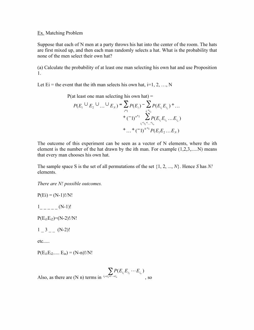
Ex. Matching Problem Suppose that each of N men at a party throws his hat into the center of the room. The hats are first mixed up, and then each man randomly selects a hat. What is the probability that none of the men select their own hat? (a) Calculate the probability of at least one man selecting his own hat and use Proposition 1. Let Ei = the event that the ith man selects his own hat, i=1, 2, …, N P(at least one man selecting his own hat) =

) ( ) 1 (

) ( ) 1 (

) ( ) ( ) (

2 1 1

1 1

2 1

2 1 2 1

2 1 2 1

N N

i i i i i i

n

N

i i i i i i N

E E E P

E E E P

E E P E P E E E P

n n

L L

L

L L

L +

< < <

+

= <

! + +

! +

+ ! = " " "

#

# #

The outcome of this experiment can be seen as a vector of N elements, where the ith element is the number of the hat drawn by the ith man. For example (1,2,3,.....N) means that every man chooses his own hat. The sample space S is the set of all permutations of the set {1, 2, ..., N}. Hence S has N! elements. There are N! possible outcomes. P(Ei) = (N-1)!/N! 1_ _ _ _ _ (N-1)! P(Ei1Ei2)=(N-2)!/N! 1 _ 3 _ _ (N-2)! etc..... P(Ei1Ei2..... Ein) = (N-n)!/N!

Also, as there are (N n) terms in !

<<<n

n

iii

iiiEEEP

L

L

21

21)(

, so

!

1

!!)!(

)!(!)(

21

21nNnnN

nNNEEEP

n

n

iii

iii=

!

!="

<<< L

L

and thus

!

1)1(

!3

1

!2

11)( 1

21N

EEEPN

N

+!+!+!=""" LL

Hence the probability that none of the N men selects their own hat, PN, is PN =

!"

#$%

&'+'+''=(((' +

!

1)1(

!3

1

!2

111)(1 1

21N

EEEPN

NLL

PN = 1/2! - 1/3! + 1/4! - ................ + (-1)^N 1/N! As N→ ∞, PN → 1/e ≈ 0.37, using exp(x) = 1 + x + x^2/2! + x^3/3! ... b) What is the probability that exactly k of the men select their won hats? To obtain the probability of exactly k matches, consider any fixed group of k men. The probability that they, and only they, select their own hats is calculated as follows: 1 2 3 ..... k _ _ _ P(Ei1Ei2..... Eik)* PN-k = (1/N)*(1/(N-1))*...*(1/(N-(k-1)))* PN-k = 1/(N*(N-1)*.....*(N-k+1)* PN-k = ((n-k)!/n!)*PN-k PN-k is the probability that the other n-k men, selecting among their own hats, have no matches. As there are (n k) choices of a set of k men, the desired probability of exactly k matches is (n k)*(n-k)!/n! PN-k = PN-k/k!

Stirling’s approximation formula for n! It’s useful to have a better sense of how n! behaves for large n. ln n! = ln 1 + ln 2 + … ln n = ∑_{k=1} ^n ln k ≅ ∫_1 ^n ln k dk = [k ln k – k]_1 ^n ≅ n ln n – n + o(n) So n! may be approximated as exp(n ln n - n) = (n^n) * exp(-n). More sophisticated methods give better approximation: ln n! ≅ n ln n – n + (1/2) ln (2πn) +o(1). Ex: n=10: ln n! = 15.104; n ln n – n + (1/2) ln (2πn) = 15.096. Ex: back to the birthday problem. Let m=365; n=# of students. p(no match) = m!/[(m-n)! m^n] ≅ exp[m ln m – m + (1/2) ln (2πm) – (m-n) ln (m-n) + m-n - (1/2) ln (2π(m-n)) – n ln m] = exp[(m-n) ln (m/(m-n)) + (1/2) ln (m/(m-n)) – n]

≅ exp[(m-n) (n/m + (1/2) (n/m)^2) + (1/2) n/m – n] ≅ exp[-n^2/2m + n/2m]

(we used Taylor expansion ln (1+x) ≅ x – x^2/2 + o(x^2) for small x.) So, prob of no match becomes small when n>>sqrt(m). Ex: (2n n) = (2n)! / (n!)(n!) ~ exp[2n ln (2n) – 2n – 2(n ln n – n)] = exp[2n ln n + 2n ln 2 – 2n – 2n ln n + 2n] = exp[2n ln 2] = 2^(2n) Ex: What about (n an), where 0<a<1? (n an) = n! / [(an)!((1-a)n)]! ~ exp[n ln n – n – an ln an + an – (1-a)n ln (1-a)n + (1-a)n] = exp[nh(a)] h(a) = -a log a – (1-a) log (1-a): often called the “entropy” function. Key function in information theory. For what a does (n an) grow most quickly? Maximize h(a): h’(a) = -ln a – 1 + log(1-a) + 1 = ln [(1-a)/a]. Setting a = ½ gives maximum: corresponds to (2n n) case considered above.